Patrick Champagne

MAE 598: Applied Computational Fluid Dynamics

Project 4

Statement on Collaboration: No Collaboration

Task 1

In this task, I was asked to model the flow over a cylinder and two ellipses. In this case, the cylinder and

ellipses were placed in a 2-D domain full of water with an inlet velocity of 3.5 cm/s. Standard values

from the Fluent Database were used. The standard laminar model was used as well. The mesh used for

all parts of this task has a resolution of 0.005m. This mesh is displayed in Figures 5 and 6. This simulation

was run for five minutes with a timestep of 0.25s. The simulation was run for 1200 timesteps at 20

iterations per timestep.

Part a)

i) The Reynolds Number for this case was calculated using the following equation:

𝑅𝑒 =𝜌𝑢𝐿

𝜇=

998.2 ∗ 0.035 ∗ 0.1

0.001003= 3483.3

Where L is the diameter of the cylinder (0.1m) and u is the flow velocity (0.035 m/s).

ii) Figures 1, 2, and 3 contain contour plots of Static Pressure, y-velocity, and stream function for the

case of flow over a cylinder. These plots also show the two-dimensional computational domain.

Figure 1. Task 1 a) Static Pressure Contour

Figure 2. Task 1 a) y-Velocity Contour

These figures show the behavior of the flow

over the cylinder. It is clear from these plots

that the flow is not steady and that there

are oscillations in the flow. These plots,

along with the line plots of lift force, show

that the flow is not steady.

iii) Figure 4 shows the line plot of lift force

on the cylinder over the last three minutes

of the five-minute simulation. For the

deliverables in this report, the “Lift Force”

report was used in Fluent. This is Option 1

as listed in the addendum to this project. As

predicted by the contours, the flow, and

therefore lift force, are unsteady. The

oscillations in lift force have an amplitude of

0.067275 N and a period of 11s.

Figure 3. Task 1 a) Stream Function Contour

Figure 4. Task 1 a) Lift Force vs. Time

Part b)

In this part of Task 1, part

a) was repeated with

ellipses instead of a

cylinder. In run 2, an

ellipse with a major axis in

the y-direction was used,

while run 3 analyzes an

ellipse with a major axis in

the x-direction.

Figures 7 and 8 show lift

force vs. time for the last

three minutes of the

simulation as in Figure 4.

As in run 1, the solutions

are oscillatory. The lift

force for Run 2 has an

amplitude of 0.1432 N and

a period of 12.75s, while

the lift force for Run 3 has

an amplitude of 0.03399 N

and a period of 9.25s.

Figure 5. Run 2 Mesh and Computational Domain

Figure 6. Run 3 Mesh and Computational Domain

Figure 8. Task 1 Run 3 Lift Force vs. Time

Figure 7. Task 1 Run 2 Lift Force vs. Time

The results from each of the three runs are presented in table 1.

Table 1

Run 1 (Cylinder) Run 2 (y-elongated ellipse) Run 3 (x-elongated ellipse)

Amplitude (N) 0.067275 0.1432 0.03399

Period (s) 11 12.75 9.25

These results show that the amplitude and period increased when the cylinder was elongated into an

ellipse along the y-axis while the period and amplitude decreased when the cylinder was elongated into

an ellipse along the x-axis.

Task 2

In this task, flow over a “flying

saucer” was modeled in Fluent.

Unlike Task 1, a full three-

dimensional simulation was used for

this task. A cylindrical wind tunnel,

with a velocity inlet on one side and

a pressure outlet on the other was

used. A parabolic velocity profile

was defined for the velocity inlet as

follows:

𝑢 = 50 (1 − (𝑟

𝑅)

2

)

Where

𝑟 = √𝑦2 + 𝑧2

The profile of the flying

saucer is defined by a

geometry file. This file was

imported as a 3D curve and

revolved around the y-axis

to create the profile. A new

plane was created with the

same origin as the system

but rotated about the z-

axis. This is the y-axis used

for the geometry. Between

runs, the angle at which this

new plane is rotated is

varied to analyze four

different angles of attack.

The profile of the saucer is

“removed” from the

computational domain

through the “Boolean”

function.

For the analysis, the

standard k-epsilon model is

utilized. The computational

domain is filled with air

with a constant density of

Figure 9. Task 2 Mesh and Computational Domain

Figure 10. Task 2 x-Velocity Contour, θ=0°

Figure 11. Task 2 x-Velocity Contour, θ=45°

0.4 kg/m^3 and a viscosity of 1.4 x 10^-5 N s

m^-2. Since a steady solution is sought,

hybrid initialization was used for each run.

Four runs are performed at tilt angles of 0,

15, 30, and 45 degrees.

The mesh used for this simulation is

displayed below. For each run, an element

size of 0.05m meters was used with the

“capture curvature” option selected. The

mesh for the 0-degree case is displayed in

Figure 9, although the same mesh settings

were used for each run.

Figures 10 and 11 show the x-velocity

contours for the 0 and 45-degree cases.

These plots show the parabolic velocity

profile at the inlet as well as the effects of

the flying saucer. Both the 0 and 45-degree cases show an acceleration of flow over the top surface of

the flying saucer followed by a low, even negative velocity downstream of the saucer. It is important to

note that the saucer has stalled aerodynamically in the 45-degree case. We can tell because of the flow

detachment which is shown in Figure 11. The lift and drag results from the simulation also back up this

observation.

For the 0, 15, and 30-degree runs, the solution converged smoothly in about 100 iterations. Monitors

were placed on lift and drag force in Fluent and the simulation was run until these values were steady.

Because the saucer has stalled in the 45-degree case, the flow is inherently unsteady. Therefore, a

steady solution cannot be obtained. In this run, the lift and drag forces oscillated and never converged

to a steady solution. This is expected as the turbulence effects result in unsteady flow under these

conditions. The Lift and Drag forces as a function of iteration are plotted in Figure 12. This last run was

run for 400 iterations, since the oscillations and residuals seemed to have stabilized by this point. In

order to determine lift and drag forces for this run, the value of one peak and trough were determined

in MATLAB. The average of these two values was then taken to be the force value for the deliverable.

The lift and drag values for each tilt angle are presented in Table 2 and plotted in Figure 13.

Table 2

Tilt Angle (°) Lift Force (N) Drag Force (N)

0 4.5958 3.1337

15 24.919 6.9503

30 52.658 20.775

45 25.409 37.753

Figure 12. Task 2 Run 2 Lift Force vs. Time

Figure 13 shows lift and drag force as a

function of tilt angle. The plot shows that

both lift and drag tend to increase as tilt

angle increases. However, between 30 and

45 degrees, lift force drops off. This is

because the surface stalls and the flow

separates, increasing drag but decreasing

lift. This phenomenon of stalling and flow

separation was discussed earlier and is

shown in Figure 11.

Figure 13. Task 2 Lift and Drag vs Tilt Angle

Task 3

In this task, flow is simulated over a

pentagonal building in a three-

dimensional domain. The domain is a

rectangular prism with the pentagon

in the middle. The inlet is set to a

constant 50 m/s velocity. The domain

is filled with air set to standard Fluent

Database settings. The outlet is set to

a pressure outlet and the remaining

surfaces are set to walls, with a

named selection being created for

the walls of the building. The

standard k-epsilon turbulence model

is used for this analysis.

The mesh used for this analysis was

set to default settings with an

element size of 0.2m. I experimented

with enabling inflation on the

building’s surface, but this yielded

similar results at the expense of time. To ensure consistency and to save time and computational power,

I used the standard 0.2m mesh for both runs. The mesh on the planes of interest for this task is

displayed in Figure 14.

Figure 14. Task 3 Mesh and Computational Domain

Run (a)

Figures 15 and 16 show the

static pressure and y-velocity

on a plane 1m above and

parallel to the ground, slicing

through the building. Figure

17 shows the y-velocity on the

plane of symmetry

perpendicular to the ground.

In this run, the flat side of the

pentagon faces the wind. It is

clear that there is a high-

pressure zone on the upwind

side of the pentagon and a

low-pressure zone on the

downwind side of the

pentagon. There is a turbulent

wake on the downwind side of

the pentagon. The flow

remains attached on three of

the five sides.

The results from Fluent

yielded a total drag force on

the building of 3610.39 N,

10.80 N due to viscous forces,

and 3599.59 N due to

pressure forces.

Figure 15. Task 3 Run (a) Horizontal Static Pressure Contour

Figure 16. Task 3 Run (a) Horizontal y-Velocity Contour

Figure 17. Task 3 Run (a) Vertical y-Velocity Contour

Run (b)

In this run, conditions are the

same except the wind is

flowing into a point of the

pentagon instead of a flat

side.

These results look similar to

the first case. There is a high-

pressure zone on the leading

edge and a turbulent low-

pressure wake. However, in

this case, the effect of the

wake is much more

pronounced and the wake is

much larger.

The results from Fluent report

a total drag value of 5323.78

N, 1.61 N of which due to

viscous forces and 5322.17 N

due to pressure.

There are distinct differences

between these cases. While it

might seem surprising that the

sharp point produces more

drag than the blunt edge, but

the plots tell an interesting

story. In Run (a), there is high

pressure on one side and low

pressure on the other four.

The difference between the

high-pressure blunt face and

low pressure on the two

downstream faces create a

net drag force in the +y

direction. However, the other

two leading edge faces are in

low pressure, therefore

decreasing the positive y

force. This explains why the

pressure drag is so much

larger in the second run. In

the second run, the two

Figure 18. Task 3 Run (b) Horizontal Static Pressure Contour

Figure 19. Task 3 Run (b) Horizontal y-Velocity Contour

Figure 20. Task 3 Run (b) Horizontal Static Pressure Contour

leading edges are in a high-pressure zone and the three trailing faces are in a low-pressure zone,

creating a force in the positive y direction with nothing to mitigate this force as in the first run.

The velocity profiles explain the difference in viscous drag between the two cases. In the first case, the

flow remains attached on the three leading faces. Because of the no-slip condition, there is a velocity

gradient in this area. This velocity gradient is steep as shown in the contour. This velocity gradient on

three of the five faces explains why the viscous forces are greater in the first run. In the second run, the

flow detaches, leading to a gentler velocity gradient and therefore less viscous drag.

Task 4

In this task, I am asked to repeat Task 1 with my chose of asymmetric “cylinder”, if area is about the

same. The goal is to see a large-amplitude response can be simulated as in Video 3 in the lecture. I ran

three cases with three different geometries. The three shapes I used were a half circle, a crescent, and a

triangle with rounded edges. Each shape was placed at the origin as in Task 1. All other settings are the

same as Task 1. I could not obtain this response in my three runs, so I will present the data for each run.

The data presented in this Task is Lift Force calculated using the automatic function in Fluent.

Run A

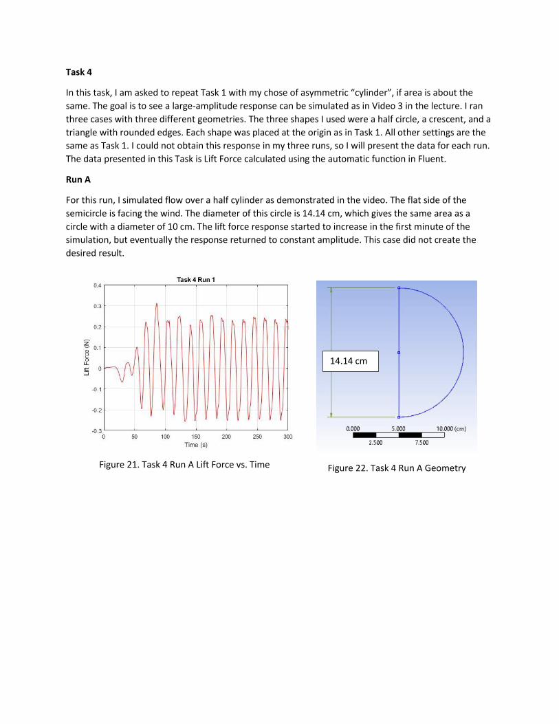
For this run, I simulated flow over a half cylinder as demonstrated in the video. The flat side of the

semicircle is facing the wind. The diameter of this circle is 14.14 cm, which gives the same area as a

circle with a diameter of 10 cm. The lift force response started to increase in the first minute of the

simulation, but eventually the response returned to constant amplitude. This case did not create the

desired result.

Figure 22. Task 4 Run A Geometry

Figure 21. Task 4 Run A Lift Force vs. Time

14.14 cm

Run B

In this case, a simple crescent was used for the geometry. To create this geometry, a semicircular arc

with a diameter of 16 cm was created. Then, an arc from three points was created, coincident with the

ends of the semicircle. The radius of the inscribed arc is defined by the distance between the center of

the arc and the origin, which is colinear with the endpoints of the semicircular arc. This dimension is

defined as 16 cm. The fluid flows from left to right, into the concave part of the crescent. The results

show that the period of the response is constant, but the amplitude is somewhat chaotic. While the

amplitude does trend upwards, the changes in amplitude between each peak is variable and

unpredictable. I do not consider this run to be a success.

Figure 24. Task 4 Run B Geometry

Figure 23. Task 4 Run B Lift Force vs. Time

16 cm

15 cm

Run C

In this run, flow was simulated over an equilateral triangle with rounded corners. The base equilateral

triangle has a side length of 15cm, and the corners have a radius of 1.75cm. This flow was the most

regular out of all three runs. The amplitude increases nearly linearly for the first four cycles and then

stays at a constant amplitude.

Figure 25. Task 4 Run C Lift Force vs. Time

Figure 26. Task 4 Run C Geometry

15 cm R = 1.75 cm