Patient-Specific Modeling and Quantification of the Aortic and Mitral ...

TO APPEAR IN IEEE TRANSACTIONS ON MEDICAL IMAGING 1

Patient-Specific Modeling and Quantificationof the Aortic and Mitral Valves from

4D Cardiac CT and TEERazvan Ioan Ionasec1,2, Ingmar Voigt1,3, Bogdan Georgescu1

Yang Wang1, Helene Houle4, Fernando Vega-Higuera5, Nassir Navab2, and Dorin Comaniciu1

1Integrated Data Systems Department, Siemens Corporate Research, Princeton NJ, USA2Computer Aided Medical Procedures, Technical University Munich, Germany3Chair of Pattern Recognition, University of Erlangen-Nuremberg, Germany

4Siemens Healthcare Ultrasound, Mountain View CA, USA5Siemens Healthcare Computed Tomography, Forchheim, Germany

Corresponding Author: Razvan Ioan Ionasec; Phone: 1-609-734-3750, Fax: 1-609-734-6565; E-mail:

[email protected]

Abstract— As decisions in cardiology increasingly rely onnon-invasive methods, fast and precise image processing toolshave become a crucial component of the analysis workflow.To the best of our knowledge, we propose the first automaticsystem for patient-specific modeling and quantification of the leftheart valves, which operates on cardiac computed tomography(CT) and transesophageal echocardiogram (TEE) data. Robustalgorithms, based on recent advances in discriminative learning,are used to estimate patient-specific parameters from sequencesof volumes covering an entire cardiac cycle. A novel physiologicalmodel of the aortic and mitral valves is introduced, whichcaptures complex morphologic, dynamic and pathologic varia-tions. This holistic representation is hierarchically defined onthree abstraction levels: global location and rigid motion model,non-rigid landmark motion model and comprehensive aortic-mitral model. First we compute the rough location and cardiacmotion applying marginal space learning. The rapid and complexmotion of the valves, represented by anatomical landmarks, isestimated using a novel trajectory spectrum learning algorithm.The obtained landmark model guides the fitting of the full phys-iological valve model, which is locally refined through learnedboundary detectors. Measurements efficiently computed from theaortic-mitral representation support an effective morphologicaland functional clinical evaluation. Extensive experiments on aheterogeneous data set, cumulated to 1516 TEE volumes from65 4D TEE sequences and 690 cardiac CT volumes from 694D CT sequences, demonstrated a speed of 4.8 seconds pervolume and average accuracy of 1.45mm with respect to expertdefined ground-truth. Additional clinical validations prove thequantification precision to be in the range of inter-user variability.To the best of our knowledge this is the first time a patient-specificmodel of the aortic and mitral valves is automatically estimatedfrom volumetric sequences.

Index Terms— Heart Valve Modeling, Heart Valve Quantifica-tion, Trajectory Spectrum Learning, Non-Rigid Motion Estima-tion, Patient-Specific Modeling

Copyright (c) 2009 IEEE. Personal use of this material is

permitted. However, permission to use this material for any

other purposes must be obtained from the IEEE by sending a

request to [email protected].

I. INTRODUCTION

Valvular surgery accounts for up to 20% of all cardiac pro-

cedures in the United States and is applied in nearly 100,000

patients every year. Yet, with an average cost of $120,000

and 5.6% in hospital death rate, valve operations are the most

expensive and riskiest cardiac interventions [1]. Aortic and

mitral valves are most commonly affected, cumulating in 64%

and 15%, respectively of all valvular heart disease (VHD)

cases [2].

The heart valves play a key role in the cardiovascular system

as they regulate the blood flow inside the heart chambers

and human body. In particular, the aortic and mitral valves

execute synchronized rapid opening and closing movements to

govern the fluid interaction in-between the left atrium (LA),

left ventricle (LV) and aorta (Ao). Their complex morpholog-

ical, functional and hemodynamical interdependency has been

recently underlined [3], [4].

Congenital, degenerative, structural, infective or inflamma-

tory diseases can provoke dysfunctions, resulting in stenotic

and regurgitant valves [5]. The blood flow is obstructed or, in

case of regurgitant valves, blood leaks due to improper closing.

Both conditions can greatly interfere with the pumping func-

tion of the heart, causing life-threatening conditions. Severe

cases require valve surgery, while mild to moderate cases need

accurate diagnosis and long-term medical management.

Precise morphological and functional knowledge about the

aortic-mitral apparatus is a prerequisite during the entire clin-

ical workflow including diagnosis, therapy-planning, surgery

or percutaneous intervention as well as patient monitoring and

follow-up. To date, most non-invasive investigations are based

on two-dimensional images, user-dependent processing and

manually performed, potentially inaccurate measurements [2].

Imaging modalities, such as Cardiac Computed Tomography

(CT) and Transesophageal Echocardiography (TEE), enable

for dynamic four dimensional scans of the beating heart over

the whole cardiac cycle. Such volumetric time-resolved data

encodes comprehensive structural and dynamic information,


(a) (b) (c)

Fig. 1. (a) Physiological model of the aortic-mitral coupling, (b) Patient-specific model fitted to CT (top) and TEE (bottom) data, (c) example of model-drivenquantification - volumes of the aortic valve sinuses over the cardiac cycle.

which however is barely exploited in clinical practice, due

to its size and complexity as well as the lack of appropriate

medical systems.

In this paper, we propose a novel system for patient-specific

modeling and clinical assessment of the aortic and mitral

valves. The robust conversion of four dimensional CT or

TEE data into relevant morphological and functional quanti-

ties comprises three aspects: physiological modeling, patient-

specific model estimation and model-driven quantification (see

Fig. 1). The aortic-mitral coupling is represented through a

mathematical model sufficiently descriptive and flexible to

capture complex morphological, dynamic and pathological

variation. It includes all major anatomic landmarks and struc-

tures and likewise it is hierarchically designed to facilitate au-

tomatic estimation of its parameters. Robust machine-learning

algorithms process the four-dimensional data coming from the

medical scanners and estimate patient-specific models of the

valves. As a result, a wide-ranging automatic analysis can be

performed to measure relevant morphological and functional

aspects of the subject valves. In that context, our major

contributions include:

• A comprehensive physiologically-driven model of the

aortic and mitral valves to capture the full morphology

and dynamics as well as pathologic variations.

• A robust and efficient method to automatically estimatevalve model parameters from four-dimensional CT or

TEE data. It includes a novel trajectory spectrum learning

algorithm for localization and motion estimation of non-

rigid objects.

• A model-driven and automatic analysis method, that

supports for morphological quantification and mea-surement of dynamic variations over the entire cardiac

cycle.

• Simultaneous analysis of the aortic-mitral complexfor concomitant clinical management and in-depth un-

derstanding of the reciprocal functional influences.

Part of this work has been reported in our conference pub-

lications [6]–[8]. In this paper, the joint valve model includes

a physiologically-driven parameterization to represent the full

morphology and dynamics of the aortic-mitral apparatus. It

also introduces a complete framework for patient-specific

parameter estimation from CT and TEE data. Moreover, a

model-based valve quantification methodology is presented

along with extensive clinical experiments. The remainder of

this paper is organized as follows: Sec. II offers an overview of

previous work on modeling and detection of cardiac structures.

The new physiological model of the aortic and mitral valves

is presented in Sec III. In Sec. IV we introduce a robust algo-

rithm for patient-specific modeling, which includes trajectory

spectrum learning and local-spatio-temporal features. Model-

driven valve quantification is presented in Sec. V. Experiments

and clinical applications are discussed in Sec. VI. This paper

concludes with Sec. VII.

II. RELATED WORK

This section presents the related work on heart valves

and cardiac models as well as object detection and motion

estimation applied to organs.

A. Cardiac and Valve Modeling

The majority of cardiac models to date are focusing on the

representation of the left (LV) and the right ventricle (RV).

More comprehensive models include also the left (LA) and

right atrium (RA) [9], ventricular outflow tracts (LVOT and

RVOT) [10], or the aorta (Ao) and pulmonary trunk (PA) [11].

Nevertheless, none of the mentioned references provides an

explicit model of the aortic or mitral valve. Existent valve

models presented in the literature are mostly generic and

used for hemodynamic studies or analysis of various pros-

theses [12]–[16]. In [17], a model of the mitral valve used for

manual segmentation of TEE data is presented. As it includes

only the mitral valve annulus and closure line during systole,

it is both static and simple. A representation of the aortic-

mitral coupling was recently proposed in [18]. This model is

dynamic but limited to only a curvilinear representation of the

aortic and mitral annuli. Due to the narrow level of detail and


insufficient parameterization, none of the existent valve models

are applicable for comprehensive patient-specific modeling or

clinical assessment.

B. Estimation of Patient-Specific Dynamic Models

The model estimation determines patient-specific param-

eters from unseen volumetric sequences. Considering the

anatomical and functional complexity of the heart valves, the

estimation procedure can be divided into two tasks: object

delineation and motion estimation.

Related approaches based on active shape models

(ASM) [19], active appearance models (AAM) [20] or de-

formable models [21], [22] are generally applied for object

delineation and segmentation [23], [24]. Often these methods

involve semi-automatic inference or require manual initial-

ization for object location. Recently, discriminative learning

methods have been proved to efficiently solve localization

problems by classifying image regions as containing a target

object. In [10], the learning based approach is applied to three-

dimensional object localization by introducing an efficient

search method referred to as marginal space learning (MSL).

To handle the large number of possible pose parameters of a

3D object, an exhaustive search of hypotheses is performed in

sub-spaces with gradually increased dimensionality.

Instead of extending discriminative learning algorithms for

time dependent four-dimensional problems, to date, motion

estimation is approached by tracking methods. To improve

robustness, many tracking algorithms integrate key frame

detection [25]. The loose coupling between detector and

tracker often outputs temporally inconsistent results. For a

more effective search, strong dynamic [26] models or sophisti-

cated statistical methods are incorporated in motion estimation

algorithms [27].

Trajectory-based features have also increasingly attracted

attention in motion analysis and recognition [28]. It has been

shown that the inherent representative power of both shape and

trajectory projections of non-rigid motion are equal, but the

representation in the trajectory space can significantly reduce

the number of parameters to be optimized [29]. This duality

has been exploited in motion reconstruction and segmenta-

tion [30], structure from motion [29]. In particular, for periodic

motion, frequency domain analysis shows promising results

in motion estimation and recognition [31], [32]. Although

the compact parameterization and duality property are crucial

in the context of learning-based object detection and motion

estimation, this synergy has not been fully exploited yet.

III. AORTIC-MITRAL PHYSIOLOGICAL MODELING

In this section we introduce our physiological model of

the aortic and mitral valves, designed to capture complex

morphological, dynamical and pathological variations. Its hi-

erarchical definition is constructed on three abstraction levels:

global location and rigid motion model, non-rigid landmark

motion model, and comprehensive aortic-mitral model. Along

with the parameterization, we introduce an anatomically driven

resampling method, to establish point correspondence required

for the construction of a statistical shape model.

(a) (b)

Fig. 2. Bounding boxes for aortic and mitral valves encoding their individualtranslation (cx, cy , cz), rotation ( �αx, �αy , �αz) and scale (sx, sy , sz). (a)Apical three chamber view, (b) aortic and mitral valves seen from the aortaand left atrium respectively, toward the LV. The green letters L,R,N andA,P indicate the L/R/N - aortic leaflets and anterior/posterior mitral leaflets,respectively.

A. Global Location and Rigid Motion Model

The global location of both aortic and mitral valves is

parameterized through the similarity transformation in the

three-dimensional space, illustrated as a bounding box in

Fig. 2. A time variable t is augmenting the representation to

capture the temporal variation during the cardiac cycle.

θ = {(cx, cy, cz), (�αx, �αy, �αz), (sx, sy, sz), t} (1)

where (cx, cy, cz), (�αx, �αy, �αz), (sx, sy, sz) are the position,

orientation and scale parameters (Fig. 2). The remainder of the

section describes the anatomically-driven definition of each

parameter in θ for both valves. Please note that the rigid

motion is modeled independently for the aortic and mitral

valves.

The aortic valve connects the left ventricular outflow tract

to the ascending aorta and includes the aortic root and three

leaflets/cusps (left (L) aortic leaflet, right (R) aortic leaflet and

none (N) aortic leaflet). The root extends from the basal ring

to the sinotubular junction and builds the supporting structure

for the leaflets. These are fixed to the root on a crown-like

attachment and can be thought of as semi-lunar pockets. The

position parameter (cx, cy, cz)aortic is given by the valve’s

barycenter, while the corresponding scale (sx, sy, sz)aorticis chosen to comprise the entire underlying anatomy. The

long axis �αz is defined by the normal vectors to the aortic

commissural plane, which is the main axis of the aortic root.

The short axis �αx is given by the normalized vector pointing

from the barycenter (cx, cy, cz)aortic to the interconnection

point of the left and right leaflet, the left/right-commissure

point. The �αy direction is constructed from the cross-product

of �αx and �αz .

Located in between the left atrium and the left ventricle,

the mitral valve includes the posterior leaflet, anterior leaflet,

annulus and subvalvular apparatus. The latter consists of the

chordae tendiae and papillary muscles, which are not explicitly


treated in this work. Hence, we compute the barycentric posi-

tion (cx, cy, cz)mitral and scale parameters (sx, sy, sz)mitral

from the mitral leaflets. �αz is described by the normal vector

to the mitral annulus, while �αx points from the barycenter

(cx, cy, cz)mitral toward the postero-annular midpoint.

In practice, the ground truth of the global location and

rigid motion model is described by the anatomical landmarks.

Landmarks and their relation to the global location and rigid

motion are defined in section III-B.

B. Non-rigid Landmark Motion Model

The aortic and mitral valves execute a rapid opening-

closing movement, which follows a complex and synchronized

motion pattern. Normalized by the time-dependent similarity

transformation introduced in Sec. III-A, the non-rigid motion

is represented through a model consisting of 18 anatomically-

defined landmarks (see Fig. 3). Three aortic commissure

points, LR-Comm, NL-Comm and RN-Comm, describe the

interconnection locations of the aortic leaflets, while three

hinges, L-Hinge, R-Hinge, and N-Hinge, are their lowest

attachment points to the root. For each leaflet of the aortic

and mitral valves, the center of the corresponding free-edge

is marked by the leaflet tip point: L/R/N-Tip tips for aortic

valves and Ant/Post-Tip (anterior/posterior) leaflet tips for

mitral valves. The two interconnection points of the mitral

leaflets at their free edges are defined by the mitral Ant/Post-

Comm, while the mitral annulus is fixed by the L/R-Trigone

and posteroannular midpoint (PostAnn MidPoint). Finally, the

interface between the aorta and coronary arteries is symbol-

ized using the L/R-Ostium, the two coronary ostia. Besides

the well defined anatomical meaning, the chosen landmarks

serve as anchor points for qualitative and quantitative clinical

assessment, are robustly identifiable by doctors and possess a

particular visual pattern.

Given the previous description, the motion of each anatom-

ical landmark j can be parameterized by its corresponding

trajectory �aj over a full cardiac cycle. For a given volume

sequence I(t), one trajectory �aj is composed by the concate-

nation of the spatial coordinates:

�aj = [�aj(0), �aj(1), · · · , �aj(t), · · · , �aj(n− 1)] (2)

where �aj are spatial coordinates with �aj(t) ∈ R3 and t an

equidistant discrete time variable t = 0, · · · , n− 1.

The anatomical landmarks are also used to describe the

global location and rigid motion, defined in Sec. III-A, as

follows: (cx, cy, cz)aortic equals to the gravity center of the

aortic landmarks, except aortic leaflet tips. �αz is the nor-

mal vector to the LR-Comm, NL-Comm, RN-Comm plane,

�αx is the unit vector orthogonal to �αz which points from

(cx, cy, cz)aortic to LR-Comm, �αy is the cross-product of �αx

and �αz . (sx, sy, sz)aortic is given by the maximal distance

between the center (cx, cy, cz)aortic and the aortic landmarks,

along each axes (�αx, �αy, �αz). Analogously to the aortic valve,

the barycentric position (cx, cy, cz)mitral is computed from the

mitral landmarks, except mitral leaflet tips. �αz is the normal

vector to the L/R-Trigone, PostAnn MidPoint plane, �αx is

orthogonal to �αz and points from (cx, cy, cz)mitral towards

(a)

(b)

(c)

Fig. 3. Anatomical landmarks of the aorto-mitral complex: (a) aorticand (b) mitral landmarks in short and long axis views, and (c) completelandmark model (See Fig. 4 for a illustration of the landmarks relation to thecomprehensive aortic-mitral model).

the PostAnn MidPoint. The scale parameters (sx, sy, sz)mitral

are defined as for the aortic valve, to comprise the entire mitral

anatomy.

C. Comprehensive Aortic-Mitral Model

The full geometry of the valves is modeled using surface

meshes constructed along rectangular grids of vertices. For

each anatomic structure a, the underlying grid is spanned along

two physiologically aligned parametric directions, �u and �v.

Each vertex �vai ∈ R3 has four neighbors, except the edge

and corner points with three and two neighbors, respectively.

Therefore, a rectangular grid with n×m vertices is represented

by (n− 1)× (m− 1)× 2 triangular faces. The model M at a


(a) (b)

(c) (d)

(e)

(f)

Fig. 4. Isolated surface components with parametric directions and spatial relations to anatomical landmarks: (a) aortic root and (b) leaflets, mitral (c) anteriorand (d) posterior leaflet. Components all together in two different cardiac phases with (e) aortic valve and opened mitral valve closed and (f) vice versa.Aortic L-, R- and N-leaflets displayed in green, cyan and red color respectively.

particular time step t is uniquely defined by vertex collections

of the anatomic structures. The time parameter t extends the

representation to capture valve dynamics:

M = [{

�va10 , · · · , �va1

N1

}︸︷︷︸

first anatomy

, · · · ,{

�van0 , · · · , �van

Nn

}︸︷︷︸

n-th anatomy

, t] (3)

where n = 6 is the number of represented anatomies and

N1 . . . Nn are the numbers of vertices for a particular anatomy.

The six represented structures are the aortic root, the three

aortic leaflets and the two mitral leaflets, which are depicted

in Fig. 4 together with their spatial relations to the anatomical

landmarks.

The aortic root connects the ascending aorta to the left

ventricle outflow tract and is represented through a tubular

grid (Fig. 4(a)). This is aligned with the aortic circumferential

u and ascending directions v and includes 36 × 20 vertices

and 1368 faces. The root is constrained by six anatomical

landmarks, i.e., three commissures and three hinges, with a

fixed correspondence on the grid. The three aortic leaflets,

the L-, R- and N-leaflet, are modeled as paraboloids on a

grid of 11 × 7 vertices and 120 faces (Fig. 4(b)). They

are stitched to the root on a crown like attachment ring,

which defines the parametric u direction at the borders. The

vertex correspondence between the root and leaflets along the

merging curve is symmetric and kept fixed. The leaflets are

constrained by the corresponding hinges, commissures and tip

landmarks, where the v direction is the ascending vector from

the hinge to the tip.The mitral leaflets separate the LA and LV hemodynami-

cally and are connected to the endocardial wall by the saddle

shaped mitral annulus. Both are modeled as paraboloids and

their upper margins define the annulus implicitly. Their grids

are aligned with the circumferential annulus direction u and

the orthogonal direction v pointing from the annulus toward

leaflet tips and commissures (Fig. 4(c) and 4(d)). The anterior

leaflet is constructed from 18×9 vertices and 272 faces while

the posterior leaflet is represented with 24 × 9 vertices and

368 faces. Both leaflets are fixed by the mitral commissures

and their corresponding leaflet tips. The left / right trigones

and the postero-annular midpoint further confine the anterior

and posterior leaflets, respectively.

D. Maintaining Spatial and Temporal ConsistencyPoint correspondence between the models from different

cardiac phases and across patients is required for building a

statistical shape model (applied in Sec. IV-C). It is difficult to

obtain and maintain a consistent parameterization as presented

in Sec. III-C in complex three-dimensional surfaces. However,

cutting planes can be applied to intersect surfaces (Fig. 5(b),

5(c) and 5(d)) and generate two-dimensional contours (Fig.

5(a)), which can be uniformly resampled using simple meth-

ods. Hence, by defining a set of physiological-based cutting


(a) (b) (c) (d) (e)

Fig. 5. (a) Example of a two-dimensional contour and corresponding uniform samples, obtained from the intersection of a plane with the three-dimensionalaortic root. Resampling planes for the mitral leaflets (b,c) and aortic root (d). The planes at the hinge and commissure levels of the aortic root in (d) aredepicted in red and green respectively. Note that for the purpose of clarity only a subset of resampling planes is visualized in figs (b),(c) and (d). (e) Leafletclosure line correction.

planes for each model component, surfaces are consistently

resampled to establish the desired point correspondence.

As mentioned in Sec. III-C the mitral annulus is a saddle

shaped curve and likewise the free edges are non-planar too.

Thus a rotation axis based resampling method is applied for

both mitral leaflets (Fig. 5(b) and 5(c)). The intersection planes

pass through the annular midpoints of the opposite leaflet.

They are rotated around the normal of the plane spanned by

the commissures and the respectively used annular midpoint.

For the aortic root (Fig. 5(d)) a pseudo parallel slice based

method is used. Cutting planes are equidistantly distributed

along the centerline following the v direction. To account

for the bending of the aortic root, especially between the

commissure and hinge level, at each location the plane normal

is aligned with the centerline’s tangent. For the aortic leaflets,

resampling of the iso-curves along their u and v directions is

found to be sufficient.

The anatomical constraints prevent leaflet intersection, dur-

ing valve closure, when leaflets are touching each other to form

the leaflet-coaptation area. Potential numerical errors, which

can accumulate at a small scale causing leaflet intersection

along the closure line, can be efficiently handled using a simple

post-processing. Given the point correspondence preserved by

the model, averaging adjacent points within the intersection

area restores model consistency and ensure high quality visu-

alization as illustrated in Fig. 5(e).

IV. PATIENT-SPECIFIC AORTIC-MITRAL MODEL

ESTIMATION

The model parameters introduced in Sec. III are esti-

mated from volumetric sequences (3D+time data), to construct

patient-specific aortic-mitral representations. We introduce a

robust learning-based algorithm, which in concordance with

the hierarchical parameterization includes three stages: global

location and rigid motion estimation, non-rigid landmark mo-

tion estimation and comprehensive aortic-mitral estimation.

Fig. 6 illustrates the entire algorithm, which relies on novel

techniques such as the trajectory spectrum learning (TSL) with

local-spatio-temporal (LST) features [6] and extends recent

machine learning methods [10], [33]. Please note that in

practice, the same framework is used for the two imaging

modalities without any modification in the algorithms, but

detectors that estimate the probabilities of model parameters

are learned separately and implicitly use modality specific

selected image features, for CT and TEE data.

A. Global Location and Rigid Motion Estimation

The location and motion parameters θ, defined in Sec. III-

A, are estimated using the Marginal Space Learning (MSL)

framework [10] in combination with Random Sample Con-

sensus (RANSAC) [34]. Given a sequence of volumes I , the

task is to find similarity parameters θ with maximum posterior

probability:

argmaxθ p(θ|I) = argmaxθp(θ(0), · · · , θ(n− 1)|I(0), · · · , I(n− 1))

(4)

To solve equation 4, we formulate the object localization

as a classification problem and estimate θ(t) for each time

step t independently, from the corresponding volumes I(t).The probability p(θ(t)|I(t)) is modeled by a learned detector

D, which evaluates and scores a large number of hypotheses

for θ(t). D is trained using the Probabilistic Boosting Tree

(PBT) [33], positive and negative samples extracted from the

ground-truth, as well as efficient 3D Haar wavelet [35] and

steerable features [10].

The object localization task is performed by scanning the

trained detector D exhaustively over all hypotheses to find

the most plausible values for θ(t) at each time step t. As

the number of hypotheses to be tested increases exponentially

with the dimensionality of the search space, a sequential

scan in a nine-dimensional, similarity transform, space is

computationally unfeasible. Suppose each dimension in θ(t)is discretized to n values, the total number of hypotheses is

n9 and even for a small n = 15 becomes extreme 3.98e+10.

To overcome this limitation, we apply the MSL framework,

which breaks the original parameters space Σ into subsets of

increasing marginal spaces:

Σ1 ⊂ Σ2 ⊂ · · · ⊂ Σn = Σ

By decomposing the original search space as follows (please

refer to Sec. III-A for a complete descriptions of the parame-

ters)

Σ1 = (cx, cy, cz)Σ2 = (cx, cy, cz, �αx, �αy, �αz)Σ3 = (cx, cy, cz, �αx, �αy, �αz, sx, sy, sz)

the target posterior probability can be expressed as:

p(θ(t)|I(t)) = p(cx, cy, cz|I(t))p(�αx, �αy, �αz|cx, cy, cz, I(t))p(sx, sy, sz|�αx, �αy, �αz, cx, cy, cz, I(t))


Fig. 6. Diagram depicting the hierarchical model estimation algorithm. Each block describes the actual estimation stage, computed model parameters andunderlying approach.

In practice, the optimal arrangement for MSL sorts the

marginal spaces in a descending order based on their variance.

Learning parameters with low variance first will decrease the

overall precision of the detection. In our case, due to CT and

TEE acquisition protocols and physiological variations of the

heart, the highest variance comes from translation followed

by orientation and scale. This order is confirmed by our

experiments to output the best results.

Instead of using a single detector D, we train detectors for

each marginal space (D1, D2 and D3) and detect by gradually

increasing dimensionality. After each stage only a limited

number of high-probability candidates are kept to significantly

reduce the search space. Experimentally determined as in [10],

100 highest score candidates are retained in Σ1, 50 in Σ2 and

25 in Σ3, such that the smallest subgroup which is likely to

include the optimal solution is preserved.

The candidates with the highest score,[θ0(0) . . . θ25(0)

]. . .

[θ0(n− 1) . . . θ25(n− 1)

], estimated

at each time step t, t = 0, . . . n − 1 are aggregated to

obtain a temporal consistent global location and motion

θ(t) by employing a RANSAC estimator. From randomly

sampled candidates, the one yielding the maximum number

of inliers is picked as the final motion. Inliers are considered

within a distance of σ = 7mm from the current candidate

and extracted at each time step t. The distance measure

d(θ(t)1, θ(t)2) is given by the maximum L1 norm of the

standard unit axis deformed by the parameters θ(t)1 and

θ(t)2, respectively. The resulting time-coherent θ(t) describes

the global location and rigid motion over the entire cardiac

cycle.

B. Non-rigid Landmark Motion Estimation

Based on the determined global location and rigid motion, in

this section we introduce a novel trajectory spectrum learning

algorithm to estimate the non-linear valve movements from

volumetric sequences. Considering the representation in sec-

tion III-B equation 2, the objective is to find for each landmark

j its trajectory �aj , with the maximum posterior probability

from a series of volumes I , given the rigid motion θ:

argmax �aj p(�aj |I, θ) = argmax �aj p(

�aj(0), · · · , �aj(n− 1)|I(0), · · · , I(n− 1), θ(0), · · · , θ(n− 1))

(5)

Note that Equ. 5 only models the non-rigid landmark motion,

as the global location and motion is removed from the trajec-

tories by aligning �aj , j = 0 . . . 10 with the aortic and �aj , j =11 . . . 17 with the mitral similarity parameters θ estimated as

described in Sec. IV-A. While it is difficult to solve equation 5

directly, various assumptions, such as the Markovian property

of the motion [36], have been proposed to the posterior

distribution over �aj(t) given images up to time t. However,

results are often not guaranteed to be smooth and may diverge

over time, due to error accumulation. These fundamental issues

can be addressed effectively if both, temporal and spatial

appearance information, is considered over the whole sequence

at once.

The trajectory representation �aj introduced in equation 2

can be uniquely represented by the concatenation of its discrete

Fourier transform (DFT) coefficients,

�sj = [�sj(0), �sj(1), · · · , �sj(n− 1)] (6)

obtained through the DFT equation:

�sj(f) =

n−1∑t=0

�aj(t)e−j2πtf

n

where �sj(f) ∈ C3 is the frequency spectrum of the x, y, and

z components of the trajectory �aj(t), and f = 0, 1, · · · , n− 1

(see Fig. 7). A trajectory �aj can be exactly reconstructed from

the spectral coefficients �sj applying the inverse DFT:

�aj(t) =

n−1∑f=0

�sj(f)ej2πtf

n (7)


(a)

2 4 8 16 32 64−0.2

−0.1

0

0.1

0.2

Components

x (real)x (imag)y (real)y (imag)z (real)z (imag)

2 4 8 16 32 64−0.2

−0.1

0

0.1

0.2

Components


2 4 8 16 32 64−0.2

−0.1

0

0.1

0.2

Components


(b)

0 10 20 30 40 50 64

−0.2−0.1

0

0.10.2

Time

xyz

0 10 20 30 40 50 64

−0.2−0.1

0

0.10.2

Time

xyz

0 10 20 30 40 50 64

−0.2−0.1

0

0.10.2

Time

xyz

(c)

Fig. 7. Example trajectories of aortic leaflet tips. (a) the aligned trajectoriesin the Cartesian space by removing the global similarity transformations.(b) corresponding 3 trajectories highlighted in red, magenta and green,which demonstrates the compact spectrum representation. (c) Reconstructedtrajectories of using 64, 10, and 3 components, respectively, showing thata small number of components can be used to reconstruct faithful motiontrajectories. The vertical axis represents the normalized motion magnitudewith respect to the reference bounding box as illustrated in Fig. 2.

The estimated trajectory is obtained using the magnitude of

the inverse DFT. From the DFT parameterization the equation

5 can be reformulated as finding the DFT spectrum �sj , with

maximal posterior probability:

argmax�sjp(�sj |I, θ) = argmax�sj

p(�sj(0), · · · , �sj(n− 1)|I(0), · · · , I(n− 1), θ(0), · · · , θ(n− 1))

(8)

Instead of estimating the motion trajectory directly, we

apply discriminative learning to detect the spectrum �sj in the

frequency domain by optimizing equation 8. The proposed

formulation benefits from three qualities:

• the DFT decomposes the trajectory space in orthogonalsubspaces, which enables the estimation of each compo-

nent �sj(f) separately.

• the DFT spectrum representation is compact, especially

for periodic motion allowing for efficient learning and

optimization.

• the posterior distribution is clustered in small regions

facilitating marginalization and pruning of the higher

dimensional parameter spaces.

Fig. 9. An example of a local-spatio-temporal feature, align with a certainposition, orientation and scale, at time t. The temporal context length of theillustrated LST feature is T, spanned symmetrical relative to t.

Inspired by the MSL reviewed in Section IV-A, we efficiently

perform trajectory spectrum learning and detection in DFT

subspaces with gradually increased dimensionality. The intu-

ition is to perform a spectral coarse-to-fine motion estimation,

where the detection of coarse level motion (low frequency) is

incrementally refined with high frequency components repre-

senting fine deformations. Section IV-B.1 presents our novel

Local-Spatio-Temporal (LST) features to incorporate both the

spatial and temporal context. The space marginalization and

training procedure of our trajectory estimator is introduced in

Section IV-B.2. Section IV-B.3 illustrates the application of

the learned detector for motion estimation from unseen data.

The trajectory spectrum learning algorithm is summarized in

Fig. 8.

1) Local-Spatio-Temporal Features: It has been shown that

local orientation and scaling of image features reduce ambigu-

ity and significantly improves learning performance [37]. We

extend the image representation by aligning contextual spatial

features in time, to capture four-dimensional information and

support motion learning from noisy data. The 4D location of

the proposed F 4D() features is parameterized by the similarity

parameters θ, defined in Sec. III-A and estimated in IV-A:

F 4D(θ(t), T |I, s) =τ(F 3D(I, θ(t+ i ∗ s)), i = −T, · · · , T ) (9)

Three-dimensional F 3D() features extract simple gradient

and intensity information from steerable pattern spatially align

with θ(t) (see [10] for the exact definition). Please note that

according to the anatomical structure, the similarity parameters

θ are defined separately for the aortic and mitral valves (see

Sec. III-B). Knowing that motion is locally coherent in time,

F 3D() is applied in a temporal neighborhood t− T to t+ Tat discrete locations evenly distributed with respect to the

current time t (see Fig. 9). The final value of a Local-

Spatial-Temporal (LST) feature is the result of time integration

using a set of linear kernels τ , which weight spatial features

F 3D() according to their distance from the current frame t.A simple example for τ , also used in our implementation, is

the uniform kernel over the interval [−T, T ], τ = 1/(2T +1)

∑Ti=−T (F

3D(I, θ(t + i ∗ s)). For this choice of τ , each

F 3D contributes equally to the F 4D.


Fig. 8. Diagram depicting the estimation of non-rigid landmark motion using trajectory spectrum learning.

The parameter T steers the size of the temporal context,

while s is a time normalization factor derived from the training

set and the number of time steps of the volume sequence I .

Values for T can be selected by the probabilistic boosting

tree (PBT) [33] in the training stage. Since the time window

size has an inverse relationship with the motion locality, the

introduced 4D local features are in consensus with a coarse-

to-fine search. Our experimental results support this property

by showing that the features with larger T values are selected

to capture the lower frequency motion, and the value of Tdecreases for higher frequency motion components.

2) Learning in Marginal Trajectory Spaces: As described

earlier, the motion trajectory is parameterized by the DFT

spectrum components �sj(f), f = 0, . . . , n − 1. Fig. 7 clearly

shows that the variation of the spectrum components decreases

substantially as the frequency increases. Consequently, trajec-

tories can be adequately approximated by a few dominant

components:

ζ ⊆ {0, . . . , n− 1}, |ζ| << n

identified during training. The obtained compact search space

can be divided in a set of subspaces. We differentiate between

two types of subspaces, individual component subspaces Σ(k)

and marginalized subspaces Σk defined as:

Σ(k) = {�s(k)} (10)

Σk = Σk−1 × Σ(k) (11)

Σ0 ⊂ Σ1 ⊂ . . . ⊂ Σr−1, r = |ζ| (12)

The subspaces Σ(k) are efficiently represented by a set of

corresponding hypotheses H(k) obtained from the training

set. The pruned search space enables efficient learning and

optimization:

Σr−1 = H(0) ×H(1) × . . .×H(r−1), r = |ζ|The training algorithm starts by learning the posterior prob-

ability distribution in the DC marginal space Σ0. Subsequently,

the learned detectors D0 is applied to identify high probable

candidates C0 from the hypotheses H(0). In the following step,

the dimensionality of the space is increased by adding the next

spectrum component (in this case the fundamental frequency,

Σ(1)). Learning is performed in the restricted space defined

by the extracted high probability regions and hypotheses set

C0 ×H(1) . The same operation is repeated until reaching the

genuine search space Σr−1.For each marginal space Σk, corresponding discriminative

classifiers Dk are trained on sets of positives Posk and

negatives Negk. We analyze samples constructed from high

probability candidates Ck−1 and hypotheses H(k). The sam-

ple set Ck−1 × H(k) is separated into positive and negative

examples by comparing the corresponding trajectories to the

ground truth in the spatial domain using the following distance

measure:

d(�aj1, �aj2) = maxt‖�aj1(t)− �aj2(t)‖

where �aj1 and �aj2 denote two trajectories for the j-th

landmark. It is important to note that the ground truth spectrum

is trimmed to the k − th component to match the dimen-

sionality of the current marginal space Σk. Given the local-

spatio-temporal features extracted from positive and negative

positions, the probabilistic boosting tree (PBT) is applied to

train a strong classifier Dk. The above procedure is repeated,

increasing the search space dimensionality in each step, until

detectors are trained for all marginal spaces Σ0, . . . ,Σr−1.3) Motion Trajectory Estimation: In this section we de-

scribe the detection procedure for object localization and

motion estimation of valve landmarks from unseen volumetric

sequences. The parameter estimation is conducted in the

marginalized search spaces Σ0, . . . ,Σr−1 using the trained

spectrum detectors D0, . . . , Dr−1 (see Section IV-B.2). Start-

ing from an initial zero-spectrum, we incrementally estimate

the magnitude and phase of each frequency component �s(k).At the stage k, the corresponding robust classifier Dk is ex-

haustively scanned over the potential candidates Ck−1×H(k).

The probability of a candidate Ck ∈ Ck−1×H(k) is computed

by the following objective function (see Fig. 8):

p(Ck) =

n−1∏t=0

Dk(IDFT (Ck), I, t) (13)

where t = 0, . . . , n − 1 is the time instance (frame index).

After each step k, the top 50 trajectory candidates Ck with high


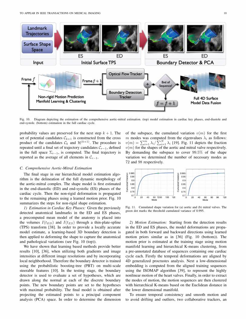
Fig. 10. Diagram depicting the estimation of the comprehensive aortic-mitral estimation. (top) model estimation in cardiac key phases, end-diastole andend-systole. (bottom) estimation in the full cardiac cycle.

probability values are preserved for the next step k + 1. The

set of potential candidates Ck+1 is constructed from the cross

product of the candidates Ck and H(k+1). The procedure is

repeated until a final set of trajectory candidates Cr−1, defined

in the full space Σr−1, is computed. The final trajectory is

reported as the average of all elements in Cr−1.

C. Comprehensive Aortic-Mitral Estimation

The final stage in our hierarchical model estimation algo-

rithm is the delineation of the full dynamic morphology of

the aortic-mitral complex. The shape model is first estimated

in the end-diastolic (ED) and end-systolic (ES) phases of the

cardiac cycle. Then the non-rigid deformation is propagated

to the remaining phases using a learned motion prior. Fig. 10

summarizes the steps for non-rigid shape estimation.

1) Estimation in Cardiac Key Phases: Given the previously

detected anatomical landmarks in the ED and ES phases,

a precomputed mean model of the anatomy is placed into

the volumes I(tED) and I(tES) through a thin-plate-spline

(TPS) transform [38]. In order to provide a locally accurate

model estimate, a learning-based 3D boundary detection is

then applied to deforming the shape to capture the anatomical

and pathological variations (see Fig. 10 (top)).

We have shown that learning based methods provide better

results [10], [36], when utilizing both gradients and image

intensities at different image resolutions and by incorporating

local neighborhood. Therefore the boundary detector is trained

using the probabilistic boosting-tree (PBT) on multi-scale

steerable features [10]. In the testing stage, the boundary

detector is used to evaluate a set of hypotheses, which are

drawn along the normal at each of the discrete boundary

points. The new boundary points are set to the hypotheses

with maximal probability. The final model is obtained after

projecting the estimated points to a principal component

analysis (PCA) space. In order to determine the dimension

of the subspace, the cumulated variation v(m) for the first

m modes was computed from the eigenvalues λi as follows:

v(m) =∑m

i=1 λi/∑N

i=1 λi [19]. Fig. 11 depicts the fraction

v(m) for the shapes of the aortic and mitral valve respectively.

By demanding the subspace to cover 99.5% of the shape

variation we determined the number of necessary modes as

72 and 98 respectively.

Fig. 11. Cumulated shape variation for (a) aortic and (b) mitral valves. Thegreen dot marks the threshold cumulated variance of 0.995.

2) Motion Estimation: Starting from the detection results

in the ED and ES phases, the model deformations are propa-

gated in both forward and backward directions using learned

motion priors similar as in [36] (Fig. 10 (bottom)). The

motion prior is estimated at the training stage using motion

manifold learning and hierarchical K-means clustering, from

a pre-annotated database of sequences containing one cardiac

cycle each. Firstly the temporal deformations are aligned by

4D generalized procrustes analysis. Next a low-dimensional

embedding is computed from the aligned training sequences

using the ISOMAP algorithm [39], to represent the highly

nonlinear motion of the heart valves. Finally, in order to extract

the modes of motion, the motion sequences are then clustered

with hierarchical K-means based on the Euclidean distance in

the lower dimensional manifold.

To ensure temporal consistency and smooth motion and

to avoid drifting and outliers, two collaborative trackers, an


optical flow tracker and a boundary detection tracker, are used

in our method. The optical flow tracker directly computes the

temporal displacement for each point from one frame to the

next. Initialized by one-step forward prediction, the detection

tracker obtains the deformations in each frame with maximal

probability. The results are then fused into a single estimate

by averaging the computed deformations and the procedure is

repeated until the full 4D model is estimated for the complete

sequence. In this way the collaborative trackers complement

each other, as the optical flow tracker provides temporally

consistent results and its major issue of drifting is addressed

by the boundary detection along with the one-step forward

prediction.

V. MODEL-BASED QUANTIFICATION OF THE

AORTIC-MITRAL APPARATUS

From the estimated patient-specific model we efficiently

derive a wide-ranging morphological and functional charac-

terization of the aortic-mitral apparatus, summarized in Tab. I.

In comparison with the gold standard, which processes 2D

images and performs manual measurements, the benefits of

the proposed automatic quantization are:

• Precision increased by modeling and measuring the nat-

ural three-dimensional valve anatomy.

• Reproducibility through automatic quantification and

avoidance of user-dependent manipulation.

• Functional assessment from dynamic measurements per-

formed over the entire cardiac-cycle.

• Comprehensive analysis including complex parameters

such as shape curvatures, deformation fields and volu-

metric variations.

Comprehensive valve measurements are important in the

clinical workflow during diagnosis and severity assessment,

surgery planning for replacement or repair and percutaneous

interventions [2]. Valvular dimensions, such as Aortic Valve

Area, Mitral valve Area and Mitral Annulus Area (Fig. 12),

automatically obtained over the whole cardiac cycle, can

benefit cardiologists in evaluating the overall structural and

functional condition. Furthermore, in-depth analysis of com-

plex pathologies can be performed through independent Sinus

Volumes quantization and Annular Deviation assessment for

the aortic and mitral valves, respectively.

Dimensions of the aortic root at the Ventriculoarterial

Junction, Valsalva Sinuses and Sinotubular Junction as well

as the Inter-ostia angle are crucial in planning for aortic

valve replacement and repair surgery [44]. These, along with

measurements of the mitral annulus and leaflets, such as

the mitral Annular circumference, Anterolateral-Posteromedial

diameter, can be automatically computed by the proposed

approach (see Fig.12)

Emerging percutaneous and minimally invasive valve in-

terventions require extensive non-invasive assessment and can

substantially benefit from the model-based quantification [40].

For instance, precise knowledge of the coronary ostia posi-

tion prevents hazardous ischemic complications by avoiding

the potential misplacement of aortic valve implants. The

method presents an integral three-dimensional configuration

TABLE I

AORTIC-MITRAL MEASUREMENTS, AUTOMATICALLY COMPUTED FROM

THE PATIENT-SPECIFIC MODEL OVER THE ENTIRE CARDIAC CYCLE

Aortic RootVentriculoarterial Junct. �,

∫,∨ [18]

Valsava Sinuses �,∫

,∨ [18]Sinotubular Junct. �,

∫,∨ [18]

Commissure-Hinge Plane ∠Sinus Volumes

Aortic LandmarksCommissure-Hinge Distance [18]Hinge-Ostium Distance [40]Ostium-Commissure DistanceInter-Commissural ∨,∠ [18]Inter-Ostia ∠

Aortic LeafletsAortic Valve

∫[40]

Coaptation Height [18]Leaflet Height [40]Effective Cusp Height [40]Leaflet Free Edge ∨ [40]Leaflet-Ostium Distance

Mitral AnnulusAnnular

∫,∨ [2], [18]

Annular Deviation Ratio [41]Annular Non-Planarity ∠ [17]Sphericity Index

Mitral LandmarksInter-Commissural Distance [2]Inter-Trigonal Distance [2]Annular-Posterior � [2]Anterolateral-Posteromedial � [2]Annular-Commissural Ratio [42]

Mitral LeafletsAnterior/Posterior Surface

∫,∨

Valve Opening∫

[2]Valve to Area RatioTenting Height and Volume [2], [43]

Aortic-MitralCentroid Distances [18]Inter-Annular ∠ [18]

� - diameter,∫

- area, ∨ - circumferential length, ∠ - angle.

of critical structures (ostia, commissures, hinges, etc.) and

calculates their relative location over the entire cardiac cycle.

Additionally, the joint model characterizes the aortic-mitral

interconnection by quantifying the Inter-Annular angle and

Centroid Distances (Fig. 12), which facilitates the challenging

management of multi-morbid patients.

It is important to notice, that the quantification potential

of the proposed method is not limited to the above mentioned

measurements. Through the consistent and comprehensive spa-

tial and temporal representation, the introduced system offers

unique analysis features, which facilitate decisions during the

whole clinical workflow. For the first time, functional and

morphological measurements can be efficiently performed for

individual valve patients and potentially improve their clinical

management.

VI. EXPERIMENTS

In this section, we demonstrate the performance of the

proposed patient-specific modeling and quantification method

for aortic and mitral valves. Experiments are performed on

a large and comprehensive data set described in Section VI-

A. In section VI-B, we demonstrate the performance of the

model estimation algorithm on cardiac CT and TEE volumetric

sequences. The clinical evaluation in VI-C presents the quan-

tification performance and accuracy for the proposed system.

A. Data Set

Functional cardiac studies were acquired using CT and

TEE scanners from 134 patients affected by various car-

diovascular diseases such as: bicuspid aortic valve, dilated

aortic root, stenotic aortic/mitral, regurgitant aortic/mitral as

well as prolapsed valves. The imaging data includes 690 CT

and 1516 TEE volumes, which were collected from medical

centers around the world over a period of two years. Using

heterogeneous imaging protocols, TEE exams were performed


(a)

(b)

Fig. 12. Examples of aortic-mitral morphological and functional measurements. (a) from left to right: aortic valve model with measurement traces, aorticvalve area, aortic root diameters and ostia to leaflets distances. (b) mitral valve with measurement traces, mitral valve and annulus area, mitral annular deviationin ED and ES and aortic-mitral angle and centroid distance.

with Siemens Acuson Sequoia (Mountain View, CA, USA) and

Philips IE33 (Andover, MA, USA) ultrasound machines while

CT scans were acquired using Siemens Somatom Sensation

or Definition scanners (Forchheim, Germany). The ECG gated

Cardiac CT sequences include 10 volumes per cardiac cycle,

where each volume contains 80-350 slices with 153× 153 to

512×512 pixels. The in-slice resolution is isotropic and varies

between 0.28 to 1.00mm with a slice thickness from 0.4 to

2.0mm. TEE data includes an equal amount of rotational (3 to

5 degrees) and matrix array acquisitions. A complete cardiac

cycle is captured in a series of 7 to 39 volumes, depending

on the patient’s heart beat rate and scanning protocol. Image

resolution and size varies for the TEE data set from 0.6 to 1

mm and 136×128×112 to 160×160×120 voxels, respectively.

The ground truth for training and testing was obtained

through an annotation process, which was guided by experts

and includes the following steps:

• the non-rigid landmark motion model is manually deter-

mined by placing each anatomical landmark (Sec. III-B)

at the correct location in the entire cardiac cycle of a

given study.

• the comprehensive aortic-mitral model is initialized

through its mean model placed at the correct image

location, expressed by the thin-plate-spline transform es-

timated from the previously annotated non-rigid landmark

motion model (see Sec. IV-C).

• the ground-truth of the comprehensive aortic-mitral

model is manually adjusted to delineate the true valves

boundary over the entire cardiac cycle.

• from the annotated non-rigid landmark motion model, the

global location and rigid motion model ground-truth is

determined as described in Sec. III-B.

Please note that while CT acquisitions contain both valves, it

is not always the case for the TEE exams, which usually focus

either on the aortic or mitral valve. Ten cases were annotated

by four distinct user for the purpose of conducting inter-user

variability study, which is presented in section VI-C. Also for a

number of four patients we obtained both, CT and TEE studies,

and used that for an inter-modality study also presented in

section VI-C.

B. Model Estimation Performance

The precision of the global location and rigid mo-

tion estimation (Sec. IV-A) is measured at the box cor-

ners of the detected time-dependent similarity transforma-

tion. Hence, the average Euclidean distance between the

eight bounding box points, defined by the similarity trans-

form (cx, cy, cz), (�αx, �αy, �αz), (sx, sy, sz), and the ground-

truth box is reported. To measure the accuracy of the non-

rigid landmark motion estimation (Sec. IV-B), detected and

ground-truth trajectories of all landmarks are compared at each

discrete time step using the Euclidean distance. The accuracy

of the surface models obtained by the comprehensive aortic-

mitral estimation (Sec. IV-C) is evaluated by utilizing the

point-to-mesh distance. For each point on a surface (mesh),

we search for the closest point (not necessarily one of the

vertices) on the other surface to calculate the Euclidean

distance. To guarantee a symmetric measurement, the point-

to-mesh distance is calculated in two directions, from detected

to ground truth surfaces and vice versa.

The performance evaluation was conducted using three-

fold cross-validation by dividing the entire dataset into three

equally sized subsets, and sequentially using two sets for

training and one for testing. Table II summarizes the model

estimation performance averaged over the three evaluation

runs. The last column represents the 80th percentile of the

error values. The estimation accuracy averages at 1.54mm and

1.36mm for TEE and CT data, respectively. On a standard

PC with a quad-core 3.2GHz processor and 2.0GB memory,

the total computation time for the tree estimation stages is 4.8


seconds per volume (approx 120sec for average length volume

sequences), from which the global location and rigid motion

estimation requires 15% of the computation time (approx

0.7sec), non-rigid landmark motion 54% (approx 2.6sec) and

comprehensive aortic-mitral estimation 31% (approx 1.5sec).

Fig. 13 shows estimation results on various pathologies for

both valves and imaging modalities.

TABLE II

ERRORS FOR EACH ESTIMATION STAGE IN TEE AND CT

TEE (in mm) Mean Std. Median 80%

Global Location and Rigid Motion 6.95 4.12 5.96 8.72Non-Rigid Landmark Motion 3.78 1.55 3.43 4.85Comprehensive Aortic-Mitral 1.54 1.17 1.16 1.78

CT (in mm) Mean Std. Median 80%

Global Location and Rigid Motion 8.09 3.32 7.57 10.4Non-Rigid Landmark Motion 2.93 1.36 2.59 3.38Comprehensive Aortic-Mitral 1.36 0.93 1.30 1.53

For the non-rigid landmark motion, we analyzed the er-

ror distribution of our approach and compared it to optical

flow [45] and tracking-by-detection [46]. Fig. 14(a) presents

the error distribution over the entire cardiac cycle, where

the end-diastolic phase is at t = 0. It can be seen that,

although performed forward and backward, the optical flow

approach is affected by drifting. In the same time, the tracking-

by-detection error is unevenly distributed, which reflects in

temporal inconsistent and noisy results. Fig. 14(b) shows the

error distribution over the 18 landmarks. Both tracking-by-

detection and optical flow perform significantly worse on

highly mobile landmarks as the aortic leaflet tips (landmarks

9, 10 and 11) and mitral leaflet tips (landmarks 15 and 16).

The proposed trajectory spectrum learning demonstrates a time

consistent and model-independent precision, superior in both

cases to reference methods.

(a) (b)

Fig. 14. Error comparison between the optical flow, tracking-by-detectionand our trajectory-spectrum approach distributed over (a) time and (b) detectedanatomical landmarks. The curve in black shows the performance of ourapproach, which has the lowest error among all three methods.

C. Quantification Performance and Clinical Evaluation

The quantification precision of the system for the mea-

surements presented in Sec. V is evaluated in comparison to

manual expert measurements. Table III shows the accuracy

for the Ventriculoarterial Junction, Valsava Sinuses and Sino-

tubular Junction aortic root diameters as well as for Annular

Circumference, Annular-Posterior Diameter and Anterolateral-

Posteromedial Diameter of the mitral valve. The Bland-Altman

plots [47] in Fig. 15 demonstrate a strong agreement between

manual and model-based measurements for aortic valve areas

and mitral annular areas.

Moreover, from a subset of 19 TEE patients, we computed

measurements of the aortic-mitral complex and compared

those to literature reported values [18]. Distances between

the centroids of the aortic and mitral annulae as well as

interannular angles were computed. The latter is the angle

between the vectors, which point from the highest point of

the anterior mitral annulus to the aortic and mitral annular

centroids respectively. The mean interannular angle and in-

terannular centroid distance were 137.0±12.2 and 26.5±4.2,

respectively compared to 136.2±12.6 and 25.0±3.2 reported

in the literature [18].

TABLE III

SYSTEM-PRECISION FOR VARIOUS DIMENSIONS OF THE AORTIC-MITRAL

APPARATUS.

Mean STD

Ventriculoarterial Junct. �(mm) 1.37 0.17Valsava Sinuses �(mm) 1.66 0.43

Sinotubular Junct. �(mm) 0.98 0.29Annular ∨(mm) 8.46 3.0

Annular-Posterior �(mm) 3.25 2.19Anterolateral-Posteromedial �(mm) 5.09 3.7

� - diameter, ∨ - circumferential length.

(a) (b)

Fig. 15. Bland-Altman plots for the (a) aortic valve area and (b) mitralannular area. The aortic valve experiments were performed on CT data from36 patients, while the mitral valve was evaluated on TEE data from 10 patients,based on the input of a expert cardiologists.

Based on a subgroup of four patients, which underwent

both, cardiac CT and TEE, we conducted an inter-modality ex-

periment. To demonstrate the consistency of the model-driven

quantification, we obtained the model and measurements from

both CT and TEE scans. We included the aortic valve area,

inter-commissural distances as well as the Ventriculoarterial

Junction, Valsava Sinuses and Sinotubular Junction diameters.

The experiment demonstrated a strong correlation r = 0.98,

p < 0.0001 and 0.97− 0.99 confidence interval.

An inter-user experiment was conducted on a randomly

selected subset of ten studies, which have their corresponding


(a)

(b)

(c) (d) (e) (f)

(g) (h) (i) (j)

Fig. 13. Examples of estimated patient-specific models from TEE and CT data: healthy valves from three different cardiac phases in (a) TEE from atrialaspect and (b) CT data in four chamber view. Pathologic valves with (c) bicuspid aortic valve, (d) aortic root dilation and regurgitation, (e) moderate aorticstenosis, (f) mitral stenosis, (g) mitral prolapse, (h) bicuspid aortic valve with prolapsing leaflets, (i) aortic stenosis with severe calcification and (j) dilatedaortic root.

patient-specific valve models manually fitted by four experi-

enced users. The inter-user variability and system error was

computed on four measurements derived from both valves,

i.e. the interannular angle and interannular centroid distance

discussed earlier in this section, performed in end-diastolic

(ED) and end-systolic (ES) phases. The inter-user variability

was determined by computing the standard deviation for each

of the four different user measurements and subsequently

averaging those to obtain the total variability. To quantify the

system error, we compare the automatic measurement result


to the mean of the different users. Fig. 16 shows the system-

error for the selected sequences with respect to the inter-user

variability. Note that except for 3% of the cases, the system-

error lies within 90% of the inter-user confidence interval.

Thus the variability of measurements obtained by different

users on the same data reveals feasible confidence intervals and

desired precision of the automated patient-specific modeling

algorithm.

Fig. 16. System error compared to the inter-user variability. The sortedsystem error (blue bars) and the 80% (light blue area) and 90% (yellow)confidence intervals of the user variability determined from the standarddeviation.

Finally, we studied our quantification performance on a pa-

tient who underwent a mitral annuloplasty procedure, intended

to reduce mitral regurgitation. Pre- and post- TEE exams were

performed before and after the successful mitral valve repair.

The measurements of the mitral valve area in Fig. 17(a)

demonstrates the regurgitant mitral valve to be cured after

procedure. Although not explicitly targeted, the intervention

had an indirect effect on the aortic valve, also illustrated in

Fig. 17(b) by the annular and valvular areas. The observation

concurs with clinical findings reported in [3], [4], [18] and

shows the converse effect to the one reported by [48], where

an intervention on the aortic affected the mitral valve.

VII. CONCLUSIONS

This paper presented a novel patient-specific modeling

and quantization framework for the aortic and mitral valves,

which comprises their full morphology and function. A

physiologically-based model allows for an anatomically cor-

rect representation of the aortic-mitral valves and their patho-

logical variations. The hierarchical definition of the model

facilitates an incremental estimation of patient-specific pa-

rameters with increased complexity. The personalized modelestimation is automatically performed applying robust and

efficient learning-based algorithms on cardiac 4D CT and TEE

data. Especially, the proposed trajectory spectrum learning

method enables the simultaneous estimation of spatio-temporal

(a)

(b)

Fig. 17. Measurements obtained before (dotted lines) and after (solid lines)mitral annuloplasty: (a) Aortic (blue) and Mitral (red) valvular area, (b) Aortic(blue) and Mitral (red) annular area.

landmark parameters, which is a central problem in computing

dynamic models.

From the patient-specific model, we compute for the first

time precise morphological and functional quantification of

the aortic-mitral complex. Extensive experiments performed

on a large heterogeneous data set demonstrated a precision

of 1.54mm on TEE data and 1.36mm on CT data at a speed

of 4.8 seconds per volume. Furthermore, clinical validation

showed a strong inter-modality and inter-subject correlation

for a comprehensive set of model-based measurements. The

method addresses problems of current clinical practice and

shows how to overcome these shortcomings. It may not only

have impact on the clinical workflow in cardiac health care,

such as diagnosis and procedural planning but also design

of prosthetic valves and percutaneous interventions for both

aortic and mitral valves and may help to understand their

interconnection and clinical implications.

ACKNOWLEDGEMENTS

The authors would like to thank all clinical collaborators:

Prof. Vannan (OSU), Prof. Schoepf (MUSC), Prof. Everett

(JHU), Prof. Lange (DHM), Prof. Pongiglione (OPBG), Prof.

Taylor (GOSH). This work has been partially funded by the

EU projects Health-e-Child (IST 2004-027749) and Sim-e-

Child.

REFERENCES

[1] W. Rosamond, K. Flegal, G. Friday, K. Furie, A. Go, K. Greenlund,N. Haase, M. Ho, V. Howard, B. Kissela, S. Kittner, D. Lloyd-Jones,M. McDermott, J. Meigs, C. Moy, G. Nichol, C.J. O’Donnell, V. Roger,J. Rumsfeld, P. Sorlie, J. Steinberger, T. Thom, S. Wasserthiel-Smoller,and Y. Hong, “Heart disease and stroke statistics–2007 update: a reportfrom the american heart association statistics committee and strokestatistics subcommittee,” Circulation, vol. 115, no. 5, pp. 69–171, 2007.

[2] R.O. Bonow, B.A. Carabello, K. Chatterjee, A.C.J. de Leon, D.P. Faxon,M.D. Freed, W.H. Gaasch, B.W. Lytle, R.A. Nishimura, P.T. OGara,R.A. ORourke, C.M. Otto, P.M. Shah, and J.S. Shanewise, “Acc/aha2006 guidelines for the management of patients with valvular heartdisease: a report of the american college of cardiology/american heartassociation task force on practice guidelines (writing committee todevelop guidelines for the management of patients with valvular heartdisease),” Circulation, vol. 114, no. 5, pp. 84–231, 2006.


[3] E. Lansac, K. Lim, Y. Shomura, W. Goetz, H. Lim, N. Rice, H. Saber,and C. Duran, “Dynamic balance of the aortomitral junction,” J ThoracCardiovasc Surg, vol. 123, pp. 911–918, 2002.

[4] T. Timek, G. Green, F. Tibayan, F. Lai, F. Rodriguez, D. Liang,G. Daughters, N. Ingels, and D. Miller, “Aorto-mitral annular dynamics,”Ann Thorac Surg, vol. 76, pp. 1944–1950, 2003.

[5] P. Libby, R.O. Bonow, D.L. Mann, and D.P. Zipes, Braunwalds’s HeartDisease: A Textbook of Cardiovascular Medicine. Elsevier, 2008.

[6] R.I. Ionasec, Y. Wang, B. Georgescu, I. Voigt, N. Navab, and D. Co-maniciu, “Robust motion estimation using trajectory spectrum learning:Application to aortic and mitral valve modeling from 4d tee,” in Proc.Int’l Conf. Computer Vision, 2009, p. in progress.

[7] R.I. Ionasec, I. Voigt, B. Georgescu, H. Houle, J. Hornegger, N. Navab,and D. Comaniciu, “Modeling and assessment of the aortic-mitral valvecoupling from 4d tee and ct,” in Proc. Int’l Conf. Medical ImageComputing and Computer Assisted Intervention, 2009, p. in progress.

[8] R.I. Ionasec, B. Georgescu, E. Gassner, S. Vogt, O. Kutter, M. Scheuer-ing, N. Navab, and D. Comaniciu, “Dynamic model-driven quantificationand visual evaluation of the aortic valve from 4d ct,” in Proc. Int’l Conf.Medical Image Computing and Computer Assisted Intervention, 2008,pp. 686 – 694.

[9] O. Ecabert, J. Peters, and J. Weese, “Modeling shape variability for fullheart segmentation in cardiac computed-tomography images,” in Proc.of SPIE Medical Imaging, vol. 7, no. 2, 2006, pp. 1199–1210.

[10] Y. Zheng, A. Barbu, B. Georgescu, M. Scheuering, and D. Comaniciu,“Four-chamber heart modeling and automatic segmentation for 3d car-diac ct volumes using marginal space learning and steerable features,”IEEE Trans. on Medical Imaging, vol. 27, no. 11, pp. 1668–1681, 2008.

[11] C. Lorenz and J. von Berg, “A comprehensive shape model of the heart,”Medical Image Analysis, vol. 10, no. 4, pp. 657–670, 2006.

[12] C.S. Peskin and D.M. McQueen, Case Studies in Mathematical Mod-eling: Ecology, Physiology, and Cell Biology. Englewood Cliffs, NJ,USA: Prentice-Hall, 1996.

[13] J. De Hart, G. Peters, P. Schreurs, and F. Baaijens, “A three-dimensionalcomputational analysis of fluidstructure interaction in the aortic valve,”Journal of Biomechanics, vol. 36, no. 1, pp. 103–10, 2002.

[14] G. Cacciola, G. Peters, and P. Schreurs, “A three-dimensional mechanicalanalysis of a stentless fibre-reinforced aortic valve prosthesis,” Journalof Biomechanics, vol. 33, no. 5, pp. 521–530, 2000.

[15] E. Votta, F. Maisano, S. Bolling, O. Alfieri, F. Montevecchi, andA. Redaelli, “The geoform disease-specific annuloplasty system: Afinite element study,” Ann Thorac Surg, vol. 84, pp. 92–101, 2007,http://dx.doi.org/10.1016/j.athoracsur.2007.03.040.

[16] X. Kuai, J. Zhang, B. Ren, F. Liu, G. Gong, and Y. Zeng,“Stress analysis on stentless quadrileaflet pericardial mitral valve,”Communications in Numerical Methods in Engineering, 2007,http://dx.doi.org/10.1002/cnm.999.

[17] F. Mahmood, S. Karthik, B. Subramaniam, P. Panzica, J. Mitchell,A. Lerner, K. Jervis, and A. Maslow, “Intraoperative application ofgeometric three-dimensional mitral valve assessment package: A fea-sibility study,” Journal of Cardiothoracic and Vascular Anesthesia,vol. 22, no. 2, pp. 292–298, 2006, http://dx.doi.org/10.1016/S0140-6736(06)69208-8.

[18] F. Veronesi, C. Corsi, L. Sugeng, V. Mor-Avi, E. Caiani, L. Weinert,C. Lamberti, and L.R.M., “A study of functional anatomy of aortic-mitralvalve coupling using 3D matrix transesophageal echocardiography,” CircCardiovasc Imaging, vol. 2, no. 1, pp. 24–31, 2009.

[19] T.F. Cootes, C.J. Taylor, D.H. Cooper, and J. Graham, “Active shapemodels—their training and application,” Computer Vision and ImageUnderstanding, vol. 61, no. 1, pp. 38–59, 1995.

[20] T.F. Cootes, G.J. Edwards, and C.J. Taylor, “Active appearance models,”IEEE Trans. Pattern Anal. Machine Intell., vol. 23, no. 6, pp. 681–685,2001.

[21] C. Corsi, G. Saracino, A. Sarti, and C. Lamberti, “Left ventricularvolume estimation for real-time three-dimensional echocardiography,”IEEE Trans. Medical Imaging, vol. 21, no. 9, pp. 1202–1208, 2002.

[22] O. Gerard, A.C. Billon, J.-M. Rouet, M. Jacob, M. Fradkin, and C. Al-louche, “Efficient model-based quantification of left ventricular functionin 3-D echocardiography,” IEEE Trans. Medical Imaging, vol. 21, no. 9,pp. 1059–1068, 2002.

[23] H.C. v. Assen, M.G. Danilouchkine, A.F. Frangi, S. Ordas, J.J.M.Westenberg, J.H.C. Reiber, and B.P.F. Lelieveldt, “SPASM: A 3DASMfor segmentation of sparse and arbitrarily oriented cardiac MRI data,”Medical Image Analysis, vol. 10, no. 2, pp. 286–303, 2006.

[24] M.d. Bruijne, B.v. Ginneken, M. Viergever, and W. Niessen, “Adaptingactive shape models for 3d segmentation of tubular structures in medicalimages,” 2003.

[25] A. Fossati, M. Dimitrijevic, V. Lepetit, and P. Fua, “Bridging the gapbetween detection and tracking for 3D monocular video-based motioncapture,” in Proc. IEEE Conf. Computer Vision and Pattern Recognition,2007.

[26] L. Taycher, D. Demirdjian, T. Darrell, and G. Shakhnarovich, “Condi-tional random people: Tracking humans with CRFs and grid filters,” inProc. IEEE Conf. Computer Vision and Pattern Recognition, 2006, pp.I: 222–229.

[27] C. Sminchisescu, A. Kanaujia, Z. Li, and D. Metaxas, “Discriminativedensity propagation for 3D human motion estimation,” in Proc. IEEEConf. Computer Vision and Pattern Recognition, 2005, pp. I: 390–397.

[28] L. Wang, X. Geng, C. Leckie, and R. Kotagiri, “Moving shape dynamics:A signal processing perspective,” in Proc. IEEE Conf. Computer Visionand Pattern Recognition, 2008, pp. 1–8.

[29] I. Akhter, Y. Sheikh, S. Khan, and T. Kanade, “Nonrigid structurefrom motion in trajectory space,” in Advances in Neural InformationProcessing Systems, 2008, pp. 41–48.

[30] L. Zelnik Manor and M. Irani, “Temporal factorization vs. spatialfactorization,” in Proc. European Conf. Computer Vision, 2004, pp. II:434–445.

[31] A. Naftel and S. Khalid, “Motion trajectory learning in the DFT-coefficient feature space,” in Proc. Int’l Conf. Computer Vision Systems,2006, p. 47.

[32] A. Briassouli and N. Ahuja, “Extraction and analysis of multiple periodicmotions in video sequences,” IEEE Trans. Pattern Anal. Machine Intell.,vol. 29, no. 7, pp. 1244–1261, 2007.

[33] Z. Tu, “Probabilistic boosting-tree: Learning discriminative methods forclassification, recognition, and clustering,” in Proc. Int’l Conf. ComputerVision, 2005, pp. 1589–1596.

[34] M. Fischler and R. Bolles, “Random sample consensus: A paradigmfor model fitting with applications to image analysis and automatedcartography,” Comm. of the ACM, vol. 24, no. 6, pp. 381–395, June1981.

[35] P. Viola and M. Jones, “Rapid object detection using a boosted cascadeof simple features,” in Proc. IEEE Conf. Computer Vision and PatternRecognition, 2001, pp. 511–518.

[36] L. Yang, B. Georgescu, Y. Zheng, P. Meer, and D. Comaniciu, “3dultrasound tracking of the left ventricle using one-step forward predictionand data fusion of collaborative trackers,” in IEEE Conference onComputer Vision and Pattern Recognition, 2008.

[37] Z. Tu, X.S. Zhou, A. Barbu, L. Bogoni, and D. Comaniciu, “Probabilistic3D polyp detection in CT images: The role of sample alignment,” inProc. IEEE Conf. Computer Vision and Pattern Recognition, 2006, pp.1544–1551.

[38] J. Duchon, “Interpolation des fonctions de deux variables suivant leprincipe de la flexion des plaques minces,” RAIRO Analyse Numerique,vol. 10, pp. 5–12, 1976.

[39] J.B. Tenenbaum, V. de Silva, and J.C. Langford, “A global geometricframework for nonlinear dimensionality reduction,” Science, vol. 290,no. 5500, pp. 2319 – 2323, 2000.

[40] M. Akhtar, E.M. Tuzcu, S.R. Kapadia, L.G. Svensson, R.K. Greenberg,E.E. Roselli, S. Halliburton, V. Kurra, P. Schoenhagen, and S. Sola,“Aortic root morphology in patients undergoing percutaneous aorticvalve replacement: Evidence of aortic root remodeling,” The Journalof Thoracic and Cardiovascular Surgery, vol. 137, no. 4, pp. 950 –956, 2009.

[41] R. Levine, M. Handschumacher, A. Sanfilippo, A.J. ans Hagege, P. Har-rigan, J. Marshall, and W.A.E., “Three-dimensional echocardiographicreconstruction of the mitral valve, with implications for mitral valveprolapse,” Circulation, vol. 80, 1989.

[42] T. Timek, J. Glasson, D. Lai, D. Liang, G. Daughters, N. Ingels, andC. Miller, “Annular height-to-commissural width ratio of annulolastyrings in vivo,” Circulation, vol. 112, pp. I–423 – I–428, 2005.

[43] J. Song, S. Fukuda, T. Kihara, M. Shin, M. Garcia, J. Thomas, andT. Shiota, “Value of mitral valve tenting volume determined by real-timethree-dimensional echocardiography in patients with functional mitralregurgitation.” American Journal of Cardiology, vol. 98, no. 8, pp. 1088–1093, 2006.

[44] T.E. David, Cardiac Surgery in the Adult : Aortic Valve Repair andAortic ValveSparing Operations. New York, NY, USA: McGraw-Hill,2008.

[45] Q. Duan, E. Angelini, S. Homma, and A. Laine, “Validation of optical-flow for quantification of myocardial deformations on simulated RT3Dultrasound,” in ISBI, 2007.

[46] T. Zhao and R. Nevatia, “3D tracking of human locomotion: a trackingas recognition approach,” in ICPR, 2002, pp. I: 546–551.


[47] J. Bland and D. Altman, “Statistical methods for assessing agreementbetween two methods of clinical measurement,” Lancet, 1986.

[48] F. Vanden-Eynden, D. Bouchard, I. El-Hamamsy, A. Butnaru, P. Demers,M. Carrier, L. Perrault, J. Tardif, and M. Pellerin, “Effect of aortic valvereplacement for aortic stenosis on severity of mitral regurgitation.” AnnThorac Surg, vol. 83, pp. 1279–84, 2007.

Patient-Specific Modeling and Quantification of the Aortic and Mitral ...

Documents

Transcript of Patient-Specific Modeling and Quantification of the Aortic and Mitral ...