Patient Prognosis from Vital Sign Time Series: CombiningConvolutional Neural Networks with a Dynamical Systems

Approach

Li-wei Lehman1, Mohammad Ghassemi1, Jasper Snoek2, and Shamim Nemati31 Massachusetts Institute of Technology, Cambridge, MA

2 Harvard School of Engineering and Applied Sciences, Cambridge, MA3 Emory University, Atlanta, GA

Abstract

In this work, we propose a stacked switching vector-autoregressive (SVAR)-CNN architecture to model thechanging dynamics in physiological time series for patientprognosis. The SVAR-layer extracts dynamical features(or modes) from the time-series, which are then fed intothe CNN-layer to extract higher-level features representa-tive of transition patterns among the dynamical modes. Weevaluate our approach using 8-hours of minute-by-minutemean arterial blood pressure (BP) from over 450 patientsin the MIMIC-II database. We modeled the time-series us-ing a third-order SVAR process with 20 modes, resultingin first-level dynamical features of size 20x480 per patient.A fully connected CNN is then used to learn hierarchicalfeatures from these inputs, and to predict hospital mortal-ity. The combined CNN/SVAR approach using BP time-series achieved a median and interquartile-range AUC of0.74 [0.69, 0.75], significantly outperforming CNN-alone(0.54 [0.46, 0.59]), and SVAR-alone with logistic regres-sion (0.69 [0.65, 0.72]). Our results indicate that includ-ing an SVAR layer improves the ability of CNNs to classifynonlinear and nonstationary time-series.

1. INTRODUCTION

Subtle dynamical patterns in physiological time-series,often difficult to observe with the bare eye, may containimportant information about the pathophysiological stateof patients and their long-term outcomes. We present anapproach to physiological time-series analysis that simul-taneously models the underlying dynamical systems usinga switching vector autoregressive (SVAR) model, and thehigh-level transition patterns among the dynamical modesusing Convolutional Neural Networks (CNNs). CNNshave been shown recently to produce state-of-the-art per-formance in image classification tasks [1]. This successis largely attributed to their ability to exploit hierarchical

structures for feature learning. However, direct applica-tion of CNNs to physiological time-series have been lim-ited due to the presence of underlying physiological con-trol systems, capable of exhibiting rich dynamical patternsat multiple time-scales.

In previous work, we adopted a SVAR process frame-work to discover the shared dynamic behaviors exhibitedin HR/BP time series of a patient cohort [2]. We usedthe proportion of time a patient spents in each of the dy-namic modes (“mode proportions” from now on) to con-struct a feature vector for predicting a patient’s underly-ing “state of health”. However, this feature does not cap-ture the high-level transition dynamic among the dynami-cal mode. To address this limitation, we propose a stackedSVAR-CNN architecture. The SVAR-layer extracts dy-namical features (or modes) from the time-series, whichare then fed into the CNN-layer to extract higher-level fea-tures representative of transition patterns among the dy-namical modes. We evaluated our approach using minute-by-minute mean arterial blood pressure (BP) of 453 ICUpatients during their first 24 hours in the ICU from theMulti-parameter Intelligent Monitoring in Intensive Care(MIMIC) II database [3].

2. Materials and Methods

This section describes the utilized dataset, as well as theSVAR and CNN architectures used to learn high-level fea-tures in the multivariate time-series of vital signs.

2.1. Dataset

Minute-by-minute mean arterial blood pressure (MAP)measurements of MIMIC II [3] adult ICU patients duringthe first 24 hours of their ICU stays were extracted. Theanalysis in this paper was restricted to 453 patients withday 1 SAPS-I scores [4] and with at least 8 hours of bloodpressure data during the first 24 hours after ICU admission.

1069ISSN 2325-8861 Computing in Cardiology 2015; 42:1069-1072.

Hospital mortality of this cohort is 14%. The data set con-tains over 9,000 hours of minute-by-minute heart rate andinvasive mean arterial blood pressure measurements (over20 hours per patient on average) from 453 adult patientscollected during the first 24 hours in the ICU. Time serieswere detrended, and Gaussian noise was used to fill in themissing or invalid values. The median age of this cohortwas 69 with an inter-quartile range of (57, 79). 59% of thepatients were male. Approximately 15% (67 out of 453) ofpatients in this cohort died in the hospital.

2.2. Switching Vector Autoregressive Mod-eling of Cohort Time Series

Our approach to discovery of shared dynamics amongpatients was based on the SVAR model [2, 5], which as-sumes there exists a library of possible dynamic behav-iors or modes; a set of multivariate autoregressive modelparameters {A(k)

p , p = 1 · · ·P}Kk=1, {Q(k)}Kk=1, whereK is the number of dynamic modes. For each mode k,A

(k)p , p = 1 · · ·P are the AR coefficient matrices (corre-

sponding to each of the P lags) and Q(k) is the correspond-ing noise covariance matrix. Let yt be the observation attime t, and zt be an indicator variable indicating the ac-tive dynamic mode at time t. Following these definitions,a SVAR model is defined by:

yt =

P∑p=1

A(zt)p yt−p +Q(zt). (1)

A collection of related time series can be modeled asswitching between these dynamic behaviors which de-scribe a locally coherent linear model that persist over asegment of time. We modeled minute-by-minute MAPtime series as a switching AR(3) process with 20 dynamicmodes as in [2]. Patients were divided into 10 training/testsets. Ten switching VAR models were learned, one foreach training set. The mode assignment of time series forpatients in the test set was inferred based on the modellearned from the corresponding training set.

2.3. Convolutional Neural Networks

Convolutional neural networks are a particular formu-lation of deep neural networks that were first developedfor the automatic classification of handwritten digits in im-ages [6]. Deep neural networks [7] are a class of mod-els which consist of a hierarchy of latent representationsdistributed across numerous simple units or neurons. Al-though each level in the hierarchy is a simple transforma-tion from the previous layer, having many units spanningmultiple layers results in a very rich latent representationthat has proven to facilitate complex tasks. Convolutionalnetworks leverage the spatio-temporal structure of the data

they model by applying a spatial or temporal convolutionof the model parameters over the input to compute the fol-lowing layer. Recently, such networks have achieved stateof the art results on image classification [1, 8] and text un-derstanding [9, 10] tasks.

The latent or hidden representation H = {h1, ..., ht}resulting from a convolutional layer in such a network iscomputed by convolving a parameterized weight matrixW over the input Z = {z1, ..., zt} followed by an ele-mentwise non-linearity g(·), i.e. H = g(W ∗ Z). This istypically repeated for multiple layers and that are followedby a final classification layer.

2.4. Combining SVAR and ConvolutionalNeural Network

We modeled the time-series using a third-order SVARprocess with 20 modes as described above. We then usedthe SVAR state marginals from the final 8 hours of theminute-by-minute BP from each patient (during their firstdays in the ICU) as input to the CNN, resulting in first-level dynamical features of size 20x480 per patient. As apre-processing step, we ordered rows of the state marginalmatrix based on the modes’ odds ratios for hospital mor-tality (from logistic regression using the training set) sothat modes with similar mortality risk share location prox-imity in the CNN input image space. A one-layer fullyconnected CNN is then used to learn hierarchical featuresfrom these inputs, and to predict hospital mortality.

As a comparison, we also use the SVAR model to learna time-series specific transition matrix among the dynamicmodes, and use the learned patient-specific transition ma-trix (20x20) as an input to CNN. This feature does notcapture the specific time of a transition, but includes in-formation regarding the frequency of transitions from onedynamical model to another, and will allow us to assessthe relative importance of transient versus global transitionfeatures of the dynamics.

The CNN kernel size is 20x20 with 12 hidden units. Ineach of the 10-fold, the training set was further divided into70%/30% training and validation set: the 70% training setwas used to build 30 different CNN models using 30 differ-ent random initializations; for each initialization, we use a5-fold validation procedure (i.e. validate the performanceof the learned CNN model using 5 different subsets of thevalidation set) to select the best CNN model for actual in-ference on the test set; the CNN model with the highestmean AUC from the 5-fold validation was used to do pre-diction on the actual test set.

1070

50 100 150 200 250 300 350 400 450

2

4

6

8

10

12

14

16

18

200

0.1

0.2

0.3

0.4

0.5

0.6

0.7

0.8

0.9

(a)Non-survivor Example

50 100 150 200 250 300 350 400 450

2

4

6

8

10

12

14

16

18

200

0.1

0.2

0.3

0.4

0.5

0.6

0.7

0.8

0.9

(b)Survivor Example

50 100 150 200 250 300 350 400 450

2

4

6

8

10

12

14

16

18

20

0.01

0.02

0.03

0.04

0.05

0.06

0.07

(c)Non-survivors Population Median

50 100 150 200 250 300 350 400 450

2

4

6

8

10

12

14

16

18

20

0.01

0.02

0.03

0.04

0.05

0.06

0.07

(d)Survivors Population Median

Figure 1. Dynamic modes state marginal probabilities over 8 hours (20x480): a comparison of the non-survivors vs. thesurvivors. Each patient was represented by a 20x480 state marginals. The x-axis represents the time (in minutes), and they-axis is the probability of belonging to different dynamic modes (20 in total). The rows were ordered based on the modes’odds ratios in ascending order, as in Table 2 (see Appendix). Low risk modes (odds ratios < 1) are on the top (rows 1 - 4),and higher risk modes (odds ratios > 1) are on the bottom (after row 5).

3. RESULTS

3.1. State Marginals from SVAR

Figure 1 shows example dynamic modes state marginalprobabilities over 8 hours (20x480) for survivors vs. non-survivors. (Top 4 rows are low-risk modes; the remainingmodes are high-risk modes.) We used univariate logisticregression analysis to test the association between the pro-portion of time patients spent in each dynamic mode (20in total) and the outcome (hospital mortality). The oddsratios from the association analysis were then used to sortthe dynamic modes.

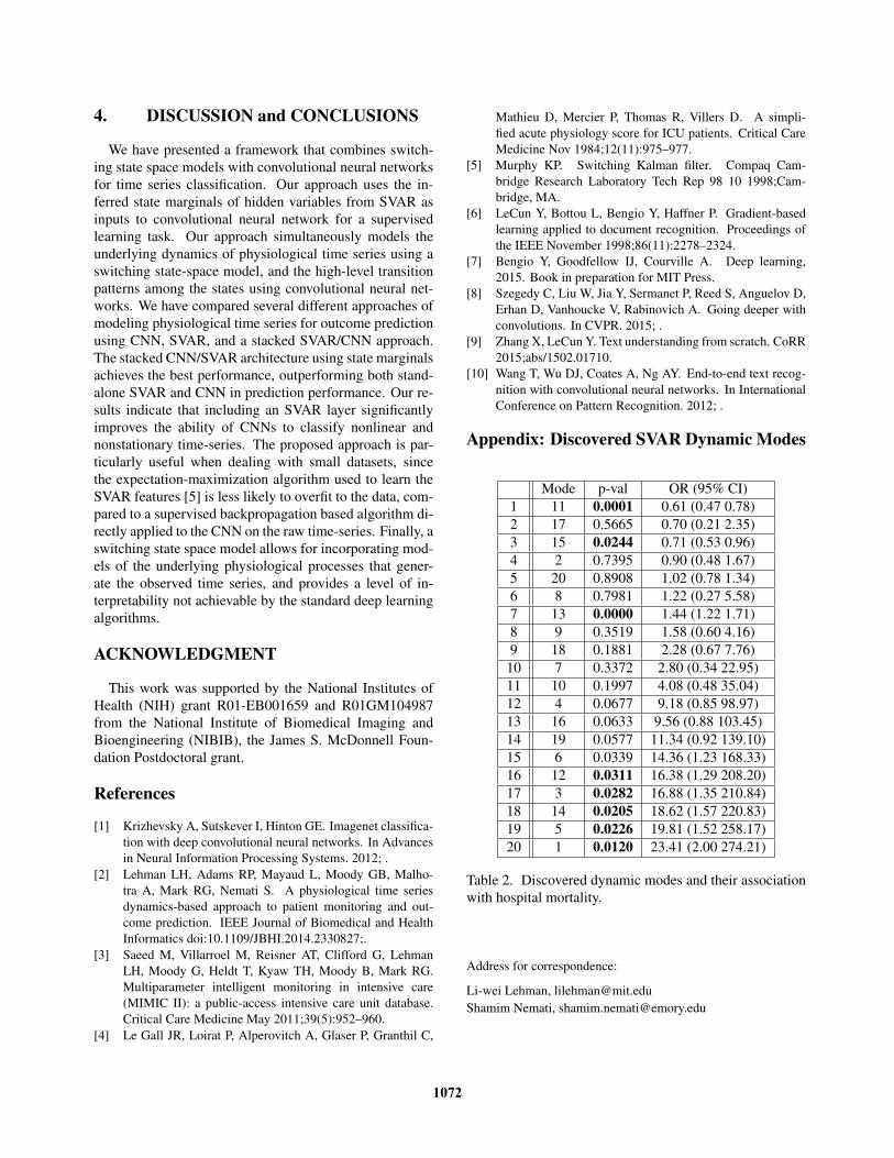
Table 2 in the Appendix shows the 20 discovered SVARdynamic modes (from one fold), listed in the order of theirassociations with hospital mortality. The same orderingis used to construct a CNN input-image from SVAR statemarginals: rows of the state marginals appear in the sameorder as the corresponding dynamic modes appear in Table2. For each mode, we report its p value, and odds ratios(OR, with 95% confidence interval) in mortality risks asper 10% increase in mode proportions. Modes are listedin ascending order based on their odds ratios. Note thatthe low-risk modes are on the top four rows; the remainingmodes are higher-risk modes with odds ratios greater thanone. Table shows the order of the dynamic modes in thestate marginal probabilities (20x480) input matrix to CNN.

3.2. Prediction Performance

Table 1 summarized the AUCs from 10-fold cross val-idation. Applying CNN-alone on the raw BP time seriesachieved an AUC of 0.54 [0.46, 0.59]. Applying logisticregression on SVAR mode proportion alone achieved anAUC of 0.69 [0.65, 0.72]. As a baseline comparison, an ex-isting acuity metric SAPS-I, using 14 different physiolog-ical/lab measurements gave an AUC of 0.65 [0.59, 0.71].

The best performance was achieved by combiningCNN/SVAR using SVAR generated state marginals fromBP time-series as an input to CNN, achieving a median andinterquartile-range AUC of 0.74 [0.69, 0.75]. Using SVARlearned patient-specific transition matrix among dynamicmodes as an input to CNN achieved a median AUC of 0.67[0.63, 0.69].

AUC (IQR)SAPS I 0.65 (0.59, 0.71)

BP Raw Samples + CNN 0.54 (0.46, 0.59)SVAR Trans. Matrix + CNN 0.67 (0.63, 0.69)

SVAR BP Dynamics MP + LR 0.69 (0.65, 0.72)SVAR BP Dynamics + CNN 0.74 (0.69, 0.75)

Table 1. Performance of Mortality Predictors. LR - logis-tic regression. MP - mode proportion.

1071

4. DISCUSSION and CONCLUSIONS

We have presented a framework that combines switch-ing state space models with convolutional neural networksfor time series classification. Our approach uses the in-ferred state marginals of hidden variables from SVAR asinputs to convolutional neural network for a supervisedlearning task. Our approach simultaneously models theunderlying dynamics of physiological time series using aswitching state-space model, and the high-level transitionpatterns among the states using convolutional neural net-works. We have compared several different approaches ofmodeling physiological time series for outcome predictionusing CNN, SVAR, and a stacked SVAR/CNN approach.The stacked CNN/SVAR architecture using state marginalsachieves the best performance, outperforming both stand-alone SVAR and CNN in prediction performance. Our re-sults indicate that including an SVAR layer significantlyimproves the ability of CNNs to classify nonlinear andnonstationary time-series. The proposed approach is par-ticularly useful when dealing with small datasets, sincethe expectation-maximization algorithm used to learn theSVAR features [5] is less likely to overfit to the data, com-pared to a supervised backpropagation based algorithm di-rectly applied to the CNN on the raw time-series. Finally, aswitching state space model allows for incorporating mod-els of the underlying physiological processes that gener-ate the observed time series, and provides a level of in-terpretability not achievable by the standard deep learningalgorithms.

ACKNOWLEDGMENT

This work was supported by the National Institutes ofHealth (NIH) grant R01-EB001659 and R01GM104987from the National Institute of Biomedical Imaging andBioengineering (NIBIB), the James S. McDonnell Foun-dation Postdoctoral grant.

References

[1] Krizhevsky A, Sutskever I, Hinton GE. Imagenet classifica-tion with deep convolutional neural networks. In Advancesin Neural Information Processing Systems. 2012; .

[2] Lehman LH, Adams RP, Mayaud L, Moody GB, Malho-tra A, Mark RG, Nemati S. A physiological time seriesdynamics-based approach to patient monitoring and out-come prediction. IEEE Journal of Biomedical and HealthInformatics doi:10.1109/JBHI.2014.2330827;.

[3] Saeed M, Villarroel M, Reisner AT, Clifford G, LehmanLH, Moody G, Heldt T, Kyaw TH, Moody B, Mark RG.Multiparameter intelligent monitoring in intensive care(MIMIC II): a public-access intensive care unit database.Critical Care Medicine May 2011;39(5):952–960.

[4] Le Gall JR, Loirat P, Alperovitch A, Glaser P, Granthil C,

Mathieu D, Mercier P, Thomas R, Villers D. A simpli-fied acute physiology score for ICU patients. Critical CareMedicine Nov 1984;12(11):975–977.

[5] Murphy KP. Switching Kalman filter. Compaq Cam-bridge Research Laboratory Tech Rep 98 10 1998;Cam-bridge, MA.

[6] LeCun Y, Bottou L, Bengio Y, Haffner P. Gradient-basedlearning applied to document recognition. Proceedings ofthe IEEE November 1998;86(11):2278–2324.

[7] Bengio Y, Goodfellow IJ, Courville A. Deep learning,2015. Book in preparation for MIT Press.

[8] Szegedy C, Liu W, Jia Y, Sermanet P, Reed S, Anguelov D,Erhan D, Vanhoucke V, Rabinovich A. Going deeper withconvolutions. In CVPR. 2015; .

[9] Zhang X, LeCun Y. Text understanding from scratch. CoRR2015;abs/1502.01710.

[10] Wang T, Wu DJ, Coates A, Ng AY. End-to-end text recog-nition with convolutional neural networks. In InternationalConference on Pattern Recognition. 2012; .

Appendix: Discovered SVAR Dynamic Modes

Mode p-val OR (95% CI)1 11 0.0001 0.61 (0.47 0.78)2 17 0.5665 0.70 (0.21 2.35)3 15 0.0244 0.71 (0.53 0.96)4 2 0.7395 0.90 (0.48 1.67)5 20 0.8908 1.02 (0.78 1.34)6 8 0.7981 1.22 (0.27 5.58)7 13 0.0000 1.44 (1.22 1.71)8 9 0.3519 1.58 (0.60 4.16)9 18 0.1881 2.28 (0.67 7.76)

10 7 0.3372 2.80 (0.34 22.95)11 10 0.1997 4.08 (0.48 35.04)12 4 0.0677 9.18 (0.85 98.97)13 16 0.0633 9.56 (0.88 103.45)14 19 0.0577 11.34 (0.92 139.10)15 6 0.0339 14.36 (1.23 168.33)16 12 0.0311 16.38 (1.29 208.20)17 3 0.0282 16.88 (1.35 210.84)18 14 0.0205 18.62 (1.57 220.83)19 5 0.0226 19.81 (1.52 258.17)20 1 0.0120 23.41 (2.00 274.21)

Table 2. Discovered dynamic modes and their associationwith hospital mortality.

Address for correspondence:

Li-wei Lehman, lilehman@mit.eduShamim Nemati, shamim.nemati@emory.edu

1072