Pathways to Net-Zero Energy Buildings: An Optimization ... · ABSTRACT Pathways to Net-Zero Energy...

Pathways to Net-Zero Energy Buildings: An OptimizationMethodology

Scott Bucking

A Thesis

In the Department

of

Building, Civil, and Environmental Engineering

Presented in Partial Fulfillment of the Requirements

For the Degree of

Doctor of Philosophy (Building Engineering) at

Concordia University

Montréal, Québec, Canada

December 2013

© Scott Bucking, 2013

Concordia UniversitySchool of Graduate Studies

This is to certify that the thesis prepared

By: Scott Bucking

Entitled: Pathways to Net-Zero Energy Buildings: An Optimization

Methodology

and submitted in partial fulfillment of the requirements for the degree of

DOCTOR OF PHILOSOPHY (Building Engineering)

complies with the regulations of the University and meets the accepted standards with

respect to originality and quality.

Signed by the final examining committee:

Dr. W.P. Zhu Chair

Dr. L. Lamarche External Examiner

Dr. N. Kharma External to Program

Dr. H. Ge Examiner

Dr. F. Haghighat Examiner

Dr. A. Athienitis Thesis Co-Supervisor

Dr. R. Zmeureanu Thesis Co-Supervisor

Approved by Dr. M. ElektorowiczGraduate Program Director

November 28, 2010 Dr. C. Trueman

Interim Dean, Faculty of Engineering and Computer Science

ii

ABSTRACT

Pathways to Net-Zero Energy Buildings: An Optimization Methodology

Scott Bucking, Ph.D.

Concordia University, 2013

Building Performance Simulation (BPS) is frequently used by decision-makers to esti-

mate building energy consumption at the design stage. However, the true potential of

BPS remains unrealized if trial and error methods of building simulation are used to

identify combinations of parameters to reduce energy use. Optimization techniques com-

bined with BPS offer many benefits such as: (i) identification of potential optimal designs

which best achieve desired performance objectives; (ii) system level component integra-

tion by simultaneously considering conflicting trade-offs; and (iii) a process-oriented

simulation tool that is complementary to BPS, eliminating the need for repetitive user-

initiated model evaluations. However, the capability of optimization algorithms to ef-

fectively map out the entire solution space and discover information is farther reaching

than building design. As shown in this thesis, optimization datasets are also a valuable

resource for conducting uncertainty and sensitivity analyses and evaluating policies to

incentivize low-energy building design.

Two performance criteria are considered in this thesis: net-energy consumption and

life-cycle cost. The term ‘performance-optimized’ refers to the extreme of these two

criteria that is Net-Zero Energy (NZE) and cost-optimized buildings. A Net-Zero Energy

Building (NZEB) generates at least as much renewable energy on-site as it consumes in

a given year. A cost-optimized building has the lowest life-cycle cost over a considered

period. A focus of this thesis is identifying optimal pathways to NZE and cost-optimized

building designs.

This thesis proposes the following approaches to identify pathways to net-zero energy:

(i) a redesign case-study of an existing near-Net-Zero Energy Home (NZEH) archetype

using a proposed optimization methodology; (ii) the development of an information-

driven hybrid evolutionary algorithm for optimal building design; (iii) a methodology

for identifying the influence of design variations on building energy performance; (iv) a

methodology to evaluate the effect of incentives on life-cycle energy-cost curves; and

(v) effect of a time-of-use feed-in tariff on optimal net-zero energy home design.

The optimization methodology consists of: (i) an energy model; (ii) a cost model;

(iii) a custom optimization algorithm; (iv) a database; and (v) a statistics module.

Several new simulation techniques are proposed to identify pathways to performance-

optimized net-zero energy buildings: (i) probability distribution functions extracted

from previous simulations; (ii) back-tracking searches; and (iii) importance factors to

summarize back-tracking search results.

This thesis provides valuable information related to: (i) the development of performance-

based energy codes for buildings; (ii) systematic design of cost-optimized NZEHs; (iii) sys-

tematic analysis of the impact of different design parameters on energy consumption and

cost; (iv) the study of incentive measures for NZEHs.

iv

Acknowledgments

I thank my supervisors, Drs. Radu Zmeureanu and Andreas Athienitis for their

patience and supervision in guiding me through a PhD. My academic training was

greatly influenced by my exposure to world class research through my participation

in conferences and IEA task meetings in Graz, Kassel, Bassel, Colorado, Barcelona and

Chambéry. I have my supervisors to thank for exposing me to such international research

events.

I thank my colleagues at the solar building research lab for their support and com-

panionship. It has been a pleasure getting to know you all thus far. I will miss our

conversations and have greatly appreciated your feedback over these past years. Special

thanks to Matthew Doiron for helping me get involved in commercial energy audits.

I would like to acknowledge several mentors and friends that have helped me through

this process: Dr. Eric Ducharme, Dr. Liam O’Brien and Dr. Lukas Swan. I acknowledge

Dr. Jose Candandedo, Constantinos Kapsis and Diane Bastien for reviewing and com-

menting on parts of this thesis. Your comments have greatly improved this document.

All of the content and concepts in this thesis were created using freely available

open-source tools. I acknowledge the creators, developers and package maintainers of:

Clojure, Python, Matplotlib, GenOpt, R-lang, ggplot, vim, texlive and SQLite.

I thank my family for keeping me grounded over the past years. Family is and

will continue to be a priority in my life. To my wife, Shannon: without your love,

encouragement, moral support and understanding a PhD would not have been possible.

Only you know how easy and yet how hard this experience has been on me. I can’t wait

for future adventures yet to come.

Table of Contents

List of Figures xi

List of Tables xv

Nomenclature xvii

Definitions xx

1 Introduction 1

1.1 Motivations . . . . . . . . . . . . . . . . . . . . . . . . . . . . . . . . . . . 1

1.2 Main Objectives . . . . . . . . . . . . . . . . . . . . . . . . . . . . . . . . 4

1.3 Scope of Thesis . . . . . . . . . . . . . . . . . . . . . . . . . . . . . . . . . 7

1.4 Thesis Overview . . . . . . . . . . . . . . . . . . . . . . . . . . . . . . . . 9

2 Literature Review 11

2.1 Overview . . . . . . . . . . . . . . . . . . . . . . . . . . . . . . . . . . . . 11

2.2 Background . . . . . . . . . . . . . . . . . . . . . . . . . . . . . . . . . . . 11

2.3 Optimization Methodology Components . . . . . . . . . . . . . . . . . . . 12

2.3.1 Objective Functions . . . . . . . . . . . . . . . . . . . . . . . . . . 13

2.3.2 Methods for Objective Function Evaluations . . . . . . . . . . . . . 15

2.3.3 Representation of Design Variables . . . . . . . . . . . . . . . . . . 18

2.3.4 Simulation File Generation . . . . . . . . . . . . . . . . . . . . . . 19

2.3.5 Optimization Algorithms . . . . . . . . . . . . . . . . . . . . . . . 21

2.3.6 Database . . . . . . . . . . . . . . . . . . . . . . . . . . . . . . . . 26

2.4 State-of-the-Art in Building Optimization Research . . . . . . . . . . . . . 27

2.4.1 Advances in Building Performance Simulation . . . . . . . . . . . . 27vi

2.4.2 Improvements to Optimization Algorithms . . . . . . . . . . . . . 30

2.4.3 Advances in the Design of Interfaces for Optimization Tools . . . . 34

2.5 Uncertainty and Sensitivity Approaches in Building Simulation . . . . . . 36

2.6 Summary of Previous Studies . . . . . . . . . . . . . . . . . . . . . . . . . 38

2.6.1 Summary of Previous Optimization Studies . . . . . . . . . . . . . 38

2.6.2 Summary of Previous Research using Uncertainty and Sensitivity

Techniques in Building Simulation . . . . . . . . . . . . . . . . . . 45

2.7 Summary . . . . . . . . . . . . . . . . . . . . . . . . . . . . . . . . . . . . 47

2.8 Overview of Research Plan . . . . . . . . . . . . . . . . . . . . . . . . . . 48

2.8.1 Objectives of PhD Thesis . . . . . . . . . . . . . . . . . . . . . . . 50

3 Concept of Design: Optimization Methodology, Energy Model, Cost

Model 52

3.1 Overview . . . . . . . . . . . . . . . . . . . . . . . . . . . . . . . . . . . . 52

3.1.1 Optimization Tool Requirements . . . . . . . . . . . . . . . . . . . 53

3.2 Concept of Design: Optimization Algorithm . . . . . . . . . . . . . . . . . 55

3.3 Evolutionary Algorithm . . . . . . . . . . . . . . . . . . . . . . . . . . . . 55

3.3.1 Representation . . . . . . . . . . . . . . . . . . . . . . . . . . . . . 56

3.3.2 Constraints . . . . . . . . . . . . . . . . . . . . . . . . . . . . . . . 57

3.3.3 Genetic Operations . . . . . . . . . . . . . . . . . . . . . . . . . . . 58

3.3.4 Selection . . . . . . . . . . . . . . . . . . . . . . . . . . . . . . . . 60

3.3.5 Diversity Definition and Control Strategy . . . . . . . . . . . . . . 61

3.3.6 Database . . . . . . . . . . . . . . . . . . . . . . . . . . . . . . . . 63

3.3.7 Multi-Objective Selection Operator . . . . . . . . . . . . . . . . . . 65

3.3.8 Core Concepts . . . . . . . . . . . . . . . . . . . . . . . . . . . . . 68

3.4 Concept of Design: Energy Model . . . . . . . . . . . . . . . . . . . . . . 75

3.4.1 Energy Balance . . . . . . . . . . . . . . . . . . . . . . . . . . . . . 77

3.4.2 Energy Objective Function . . . . . . . . . . . . . . . . . . . . . . 85

3.4.3 Energy Model Details . . . . . . . . . . . . . . . . . . . . . . . . . 86

3.5 Concept of Design: Cost Model . . . . . . . . . . . . . . . . . . . . . . . . 103

3.5.1 Cost Calculation Procedures . . . . . . . . . . . . . . . . . . . . . 103

vii

3.5.2 Life-Cycle Period . . . . . . . . . . . . . . . . . . . . . . . . . . . . 106

3.5.3 Salvage Values . . . . . . . . . . . . . . . . . . . . . . . . . . . . . 106

3.5.4 Material Initial and Replacement Costs . . . . . . . . . . . . . . . 107

3.5.5 Miscellaneous Costs . . . . . . . . . . . . . . . . . . . . . . . . . . 113

3.5.6 Income Generation: Feed-in Tariffs . . . . . . . . . . . . . . . . . . 114

3.5.7 Utility Rates and Operation Costs . . . . . . . . . . . . . . . . . . 115

3.5.8 Location Cost Multipliers . . . . . . . . . . . . . . . . . . . . . . . 117

3.5.9 Other Economic Metrics . . . . . . . . . . . . . . . . . . . . . . . . 117

3.6 Concept of Design: Summary . . . . . . . . . . . . . . . . . . . . . . . . . 120

4 Multi-Objective Optimal Design of a Near Net-Zero Energy Solar

House 121

4.1 Overview . . . . . . . . . . . . . . . . . . . . . . . . . . . . . . . . . . . . 121

4.2 Background . . . . . . . . . . . . . . . . . . . . . . . . . . . . . . . . . . . 122

4.3 Method and Problem Formulation . . . . . . . . . . . . . . . . . . . . . . 124

4.4 Energy and Cost Model . . . . . . . . . . . . . . . . . . . . . . . . . . . . 126

4.5 Optimization Algorithm . . . . . . . . . . . . . . . . . . . . . . . . . . . . 126

4.6 Results and Discussion . . . . . . . . . . . . . . . . . . . . . . . . . . . . . 128

5 An Information Driven Hybrid Evolutionary Algorithm for Optimal

Building Design 135

5.1 Overview . . . . . . . . . . . . . . . . . . . . . . . . . . . . . . . . . . . . 135

5.2 Background . . . . . . . . . . . . . . . . . . . . . . . . . . . . . . . . . . . 135

5.3 Methodology . . . . . . . . . . . . . . . . . . . . . . . . . . . . . . . . . . 136

5.3.1 Proposed Optimization Algorithms . . . . . . . . . . . . . . . . . . 137

5.3.2 Optimization Algorithm Performance Comparison . . . . . . . . . 140

5.4 Case Study: Net-Zero Energy House . . . . . . . . . . . . . . . . . . . . . 141

5.4.1 Objective function . . . . . . . . . . . . . . . . . . . . . . . . . . . 141

5.4.2 Cost Constraint . . . . . . . . . . . . . . . . . . . . . . . . . . . . . 142


5.6 Conclusions . . . . . . . . . . . . . . . . . . . . . . . . . . . . . . . . . . . 148

viii

6 A Methodology for Identifying the Influence of Design Variations on

Building Energy Performance 150

6.1 Overview . . . . . . . . . . . . . . . . . . . . . . . . . . . . . . . . . . . . 150

6.2 Background . . . . . . . . . . . . . . . . . . . . . . . . . . . . . . . . . . . 151

6.3 Methodology . . . . . . . . . . . . . . . . . . . . . . . . . . . . . . . . . . 151

6.3.1 Formation of PDFs from an Optimization Training Dataset . . . . 152

6.3.2 Monte Carlo Analysis . . . . . . . . . . . . . . . . . . . . . . . . . 155

6.3.3 Calculation of Importance Factors using Back-tracking Searches . 156

6.4 Case Study . . . . . . . . . . . . . . . . . . . . . . . . . . . . . . . . . . . 159

6.5 Results . . . . . . . . . . . . . . . . . . . . . . . . . . . . . . . . . . . . . . 160

6.6 Discussion and Conclusion . . . . . . . . . . . . . . . . . . . . . . . . . . . 165

7 Optimization Methodology to Evaluate the Effect Size of Incentives on

Life-Cycle Cost for NZEHs 169

7.1 Overview . . . . . . . . . . . . . . . . . . . . . . . . . . . . . . . . . . . . 169

7.2 Background . . . . . . . . . . . . . . . . . . . . . . . . . . . . . . . . . . . 170

7.3 Method: Evaluating in Effect Size of Incentives on NZEH Design Opti-

mization . . . . . . . . . . . . . . . . . . . . . . . . . . . . . . . . . . . . . 173


7.5 Conclusion . . . . . . . . . . . . . . . . . . . . . . . . . . . . . . . . . . . 182

8 Effect of a Time-of-Use Feed-In Tariff on Optimal Net-Zero Energy

Home Design 184

8.1 Overview . . . . . . . . . . . . . . . . . . . . . . . . . . . . . . . . . . . . 184

8.2 Background . . . . . . . . . . . . . . . . . . . . . . . . . . . . . . . . . . . 185

8.3 Method . . . . . . . . . . . . . . . . . . . . . . . . . . . . . . . . . . . . . 186


8.5 Conclusion . . . . . . . . . . . . . . . . . . . . . . . . . . . . . . . . . . . 191

9 Conclusion 193

9.1 Summary . . . . . . . . . . . . . . . . . . . . . . . . . . . . . . . . . . . . 193

9.2 Contributions . . . . . . . . . . . . . . . . . . . . . . . . . . . . . . . . . . 195

ix

9.3 Future Work . . . . . . . . . . . . . . . . . . . . . . . . . . . . . . . . . . 196

9.4 Final Thoughts . . . . . . . . . . . . . . . . . . . . . . . . . . . . . . . . . 199

References 201

Appendices 220

A Uncertainty and Sensitivity Analysis of Cost Model 220

A.1 Method . . . . . . . . . . . . . . . . . . . . . . . . . . . . . . . . . . . . . 220

A.2 Results and Discussion . . . . . . . . . . . . . . . . . . . . . . . . . . . . . 222

A.3 Conclusion . . . . . . . . . . . . . . . . . . . . . . . . . . . . . . . . . . . 224

B Description of Optimization Software 226

B.1 Overview . . . . . . . . . . . . . . . . . . . . . . . . . . . . . . . . . . . . 226

B.2 Software Structure . . . . . . . . . . . . . . . . . . . . . . . . . . . . . . . 226

B.3 Algorithm Scalability Tests . . . . . . . . . . . . . . . . . . . . . . . . . . 229

B.3.1 Method . . . . . . . . . . . . . . . . . . . . . . . . . . . . . . . . . 230

B.3.2 Scalability Results and Discussion . . . . . . . . . . . . . . . . . . 231

C Formation of Reference Building 232

C.1 Overview . . . . . . . . . . . . . . . . . . . . . . . . . . . . . . . . . . . . 232

x

List of Figures

2.1 Optimization flow chart . . . . . . . . . . . . . . . . . . . . . . . . . . . . 12

2.2 Example of templating substitutions using the BEOpt macro language in

an EnergyPlus IDF file (Anderson et al., 2006; Christensen et al., 2004) . 20

3.1 EA flowchart . . . . . . . . . . . . . . . . . . . . . . . . . . . . . . . . . . 55

3.2 Bit-by-bit uniform recombination (modified from Eiben and Smith (2003)) 59

3.3 Variable uniform recombination . . . . . . . . . . . . . . . . . . . . . . . . 60

3.4 Demonstration of diversity calculation for a single individual . . . . . . . 62

3.5 Convergence and spreading in the NSGAII selection operator (Magnier,

2009) . . . . . . . . . . . . . . . . . . . . . . . . . . . . . . . . . . . . . . . 66

3.6 NSGA-II distance calculation (Deb, 2001) . . . . . . . . . . . . . . . . . . 67

3.7 NSGA-II selection procedure (Deb, 2001) . . . . . . . . . . . . . . . . . . 67

3.8 Growing population using (μ + λ) selection operators . . . . . . . . . . . . 68

3.9 Simplified back-tracking search of vector A back-tracked to reference de-

sign vector B . . . . . . . . . . . . . . . . . . . . . . . . . . . . . . . . . . 69

3.10 Formation of contours from solution space (Feoktistov, 2006) . . . . . . . 70

3.11 Navigation of solution spaces using repeated sequential searches (modified

from Feoktistov (2006) . . . . . . . . . . . . . . . . . . . . . . . . . . . . . 70

3.12 Deterministic versus probabilistic models (Heo et al., 2011) . . . . . . . . 72

3.13 Emergent properties of PDFs with EUI reductions . . . . . . . . . . . . . 73

3.14 Energy flow paths in a typical building (Clarke, 2001) . . . . . . . . . . . 76

3.15 Inside surface heat balance diagram (DOE, 2011b) . . . . . . . . . . . . . 80

3.16 EnergyPlus Integrated Solution Manager (DOE, 2011b) . . . . . . . . . . 82

xi

3.17 Matrix formation of future-time coefficients (A) for a single thermal zone,

where Aθn+1 = Bθn + C (Clarke, 2001) . . . . . . . . . . . . . . . . . . . 83

3.18 Sparse matrix for systems solution to building heat loss in four zone

model (Clarke, 2001) . . . . . . . . . . . . . . . . . . . . . . . . . . . . . . 84

3.19 Peak electricity usage for various user profiles (Armstrong et al., 2009) . . 88

3.20 Breakdown of occupant loads into daily internal gain profiles (O’Brien,

2011) . . . . . . . . . . . . . . . . . . . . . . . . . . . . . . . . . . . . . . . 88

3.21 Relation of azimuth to peak solar gains (Modified from Henderson and

Roscoe (2010)) . . . . . . . . . . . . . . . . . . . . . . . . . . . . . . . . . 90

3.22 Moisture treatment of the wall envelope (Lstiburek, 2009) . . . . . . . . . 91

3.23 Construction of a double 2x4" wall (courtesy of Habitat Studio) . . . . . . 91

3.24 Section of common and raised roof trusses . . . . . . . . . . . . . . . . . . 92

3.25 Section of basement configuration (O’Brien, 2011) . . . . . . . . . . . . . 93

3.26 Effect of thermal zoning on electrical energy-consumption (O’Brien, 2011) 94

3.27 Temperature dead-band from monitored data in the ÉcoTerra solar

home (Modified from Doiron (2010)) . . . . . . . . . . . . . . . . . . . . . 97

3.28 Heat-gain for various window types during heating season (O’Brien, 2011) 99

3.29 Window awning . . . . . . . . . . . . . . . . . . . . . . . . . . . . . . . . . 99

3.30 Blower door setup (Krarti, 2011) . . . . . . . . . . . . . . . . . . . . . . . 100

3.31 Schematic of PV cell: Four parameter diode model (EnergyPlus engineer-

ing manual, (DOE, 2011b)) . . . . . . . . . . . . . . . . . . . . . . . . . . 102

3.32 Salvage values: Linear depreciation of initial and replacement costs . . . . 107

3.33 Diagram of 10kW grid connected Photovoltaic (PV) system (RSMeans,

2012) . . . . . . . . . . . . . . . . . . . . . . . . . . . . . . . . . . . . . . . 112

3.34 Example PV system life-cycle: Feed-in tariff and salvage value . . . . . . 112

3.35 Example cash flow diagram of optimal design compared to reference design120

4.1 ÉcoTerra House. . . . . . . . . . . . . . . . . . . . . . . . . . . . . . . . 122

4.2 ÉcoTerra annual energy consumption (Doiron et al., 2011). . . . . . . . 123

4.3 ÉcoTerra System schematic (Chen, 2009). . . . . . . . . . . . . . . . . . 123

4.4 Multi-objective constrained redesign of ÉcoTerra home. . . . . . . . . . 128

xii

4.5 Multi-objective complete redesign of ÉcoTerra home. . . . . . . . . . . 129

4.6 ÉcoTerra annual energy consumption compared to optimal design (Mod-

ified from Doiron (2010)). . . . . . . . . . . . . . . . . . . . . . . . . . . . 130

4.7 Average of 20 runs of the baseline EA . . . . . . . . . . . . . . . . . . . . 131

4.8 Average of 20 runs of hybrid EA . . . . . . . . . . . . . . . . . . . . . . . 132

4.9 Dendrogram of variable interactions where inverse mutual information

is used as a distance metric, using agglomerative clustering (complete

method with Canberra distance) . . . . . . . . . . . . . . . . . . . . . . . 133

4.10 Back-tracking search from initial ÉcoTerra design to global optimum . 134

5.1 Overview of the proposed mutual information evolutionary algorithm

(MIHEA) . . . . . . . . . . . . . . . . . . . . . . . . . . . . . . . . . . . . 139

5.2 Simulation scalability test on NZEH energy model . . . . . . . . . . . . . 145

5.3 Box-whisker plot for 20 optimization runs . . . . . . . . . . . . . . . . . . 148

6.1 Formation of PDFs from the optimization dataset . . . . . . . . . . . . . . 153

6.2 Kernel density function fitted to discrete probabilities of one variable . . . 154

6.3 Monte Carlo analysis . . . . . . . . . . . . . . . . . . . . . . . . . . . . . . 156

6.4 Calculation of importance factors using back-tracking searches . . . . . . 157

6.5 Sample of PDFs extracted from the training dataset . . . . . . . . . . . . 161

6.6 Probability of occurrence for southern WWR and wall insulation param-

eters resulting in homes that are NZE compliant . . . . . . . . . . . . . . 161

6.7 Histogram of 1000 samples from the Monte Carlo analysis . . . . . . . . . 162

6.8 Back-tracking of one NZE non-compliant design to the reference building 163

6.9 Plot of importance factor mean and standard deviation . . . . . . . . . . 165

6.10 Convergence characteristics for the five most influence variables towards

a constant importance factor . . . . . . . . . . . . . . . . . . . . . . . . . 165

7.1 Energy-cost optimal curves in BEOpt (modified from Christensen et al.

(2004)) . . . . . . . . . . . . . . . . . . . . . . . . . . . . . . . . . . . . . . 171

7.2 Identification of cost optimal and cost neutral buildings (modified from BPIE

(2010)) . . . . . . . . . . . . . . . . . . . . . . . . . . . . . . . . . . . . . . 172

xiii

7.3 Distribution of air-tightness in the Canadian housing stock . . . . . . . . 174

7.4 Identification of a cost-equivalent design . . . . . . . . . . . . . . . . . . . 175

7.5 Incentive effect using a energy-cost diagram . . . . . . . . . . . . . . . . . 175

7.6 Energy-cost curve: No incentives . . . . . . . . . . . . . . . . . . . . . . . 179

7.7 4-point diagrams for various incentives . . . . . . . . . . . . . . . . . . . . 179

7.8 Energy-cost curve: PV feed-in tariff . . . . . . . . . . . . . . . . . . . . . 180

8.1 Cash flow diagram of optimal design using FIT incentive and mortgage . 188

8.2 Cash flow diagram: Optimal design compared to reference building . . . . 189

8.3 Cash flow diagram: Optimal design compared to reference building. Util-

ity prices at 14¢/kWh. . . . . . . . . . . . . . . . . . . . . . . . . . . . . . 190

8.4 Cash flow diagram: Optimal design compared to reference building. PV

prices at 1.0$/W and electricity prices at 14¢/kWh. . . . . . . . . . . . . . 191

A.1 Monte Carlo distribution of results: Net-present value . . . . . . . . . . . 223

A.2 Monte Carlo distribution of results: Capital payback . . . . . . . . . . . . 224

B.1 Software dependency graph . . . . . . . . . . . . . . . . . . . . . . . . . . 228

B.2 Approach for optimization algorithm scalability test (Eiben and Smith,

2003) . . . . . . . . . . . . . . . . . . . . . . . . . . . . . . . . . . . . . . . 230

B.3 Optimization algorithm scalability test. Comparing proposed evolution-

ary algorithm to GenOpt PSOIW . . . . . . . . . . . . . . . . . . . . . . . 231

C.1 Distribution of construction dates . . . . . . . . . . . . . . . . . . . . . . . 233

C.2 Distribution of residential air-tightness . . . . . . . . . . . . . . . . . . . . 233

C.3 Window-to-Wall ratio trends for homes constructed after 1980 . . . . . . . 234

C.4 Distribution of wall insulation . . . . . . . . . . . . . . . . . . . . . . . . . 235

C.5 Distribution of attic insulation . . . . . . . . . . . . . . . . . . . . . . . . 235

C.6 Distribution of basement wall insulation . . . . . . . . . . . . . . . . . . . 236

C.7 Distribution of slab insulation . . . . . . . . . . . . . . . . . . . . . . . . . 236

xiv

List of Tables

3.1 Overview of optimization methodology . . . . . . . . . . . . . . . . . . . . 53

3.2 Comparison of numerical encoding of representations . . . . . . . . . . . . 57

3.3 Database table ‘indiv’ for representation simulation results . . . . . . . . . 64

3.4 Database table ‘vmap’ for variable representation . . . . . . . . . . . . . . 64

3.5 Window properties used in energy model (O’Brien, 2011) . . . . . . . . . 98

3.6 Incremental costing data for wall construction . . . . . . . . . . . . . . . . 108

3.7 Incremental costing data for ceiling construction . . . . . . . . . . . . . . 108

3.8 Costing data for concrete floor and wall construction . . . . . . . . . . . . 109

3.9 Window costing data . . . . . . . . . . . . . . . . . . . . . . . . . . . . . . 110

3.10 Costing data for gable roofs at various pitches . . . . . . . . . . . . . . . . 110

3.11 Envelope air-tightness: combined labour and material costs . . . . . . . . 111

3.12 Material and labour costs for a 10kW grid connected PV system (RSMeans,

2012) . . . . . . . . . . . . . . . . . . . . . . . . . . . . . . . . . . . . . . . 113

3.13 Replacement cost and serviceable life-cycle of materials . . . . . . . . . . 114

3.14 Time of use billing . . . . . . . . . . . . . . . . . . . . . . . . . . . . . . . 116

3.15 RSMeans location multipliers (RSMeans, 2013) . . . . . . . . . . . . . . . 117

4.1 Definition of optimization variables and parameters used for the Ecoterra

redesign study . . . . . . . . . . . . . . . . . . . . . . . . . . . . . . . . . 126

4.2 Summary of algorithm configuration . . . . . . . . . . . . . . . . . . . . . 127

5.1 Sample of influential variables for NZEH case study . . . . . . . . . . . . 142

5.2 Sample of grey-coded binary representation of design variables . . . . . . 142

5.3 Parametric run for various algorithm parameters, EA . . . . . . . . . . . . 144

5.4 Parametric run for various algorithm parameters, GenOpt PSOIW . . . . 144xv

5.5 Expected optimal fitness for the proposed EA, proposed MIHEA and

PSOIW based on 20 repeated optimization runs, NZEH case study . . . . 145

5.6 Optimization results with MIHEA: Optimal design for case study . . . . . 146

5.7 Search probability of design variable within MIHEA for Case Study . . . 147

6.1 Sample of influential model variables for a NZEH . . . . . . . . . . . . . . 160

6.2 Importance factors for influential variables . . . . . . . . . . . . . . . . . . 164

7.1 Definition of reference building . . . . . . . . . . . . . . . . . . . . . . . . 176

7.2 Summary of life-cycle cost parameters . . . . . . . . . . . . . . . . . . . . 176

7.3 Summary of multi-objective algorithm configuration . . . . . . . . . . . . 177

7.4 Cost optimal design using the PV FIT incentive . . . . . . . . . . . . . . 181

7.5 Energy and cost values for reference cost optimal and cost equivalent

buildings . . . . . . . . . . . . . . . . . . . . . . . . . . . . . . . . . . . . . 181

7.6 Initial cost premiums for cost-optimal design using various incentives . . . 182

8.1 Time of use Feed-in Tariff . . . . . . . . . . . . . . . . . . . . . . . . . . . 186

8.2 Optimization Results for ÉcoTerra Complete Redesign . . . . . . . . . 187

8.3 Sample of capital payback of design upgrades from reference to optimal

design . . . . . . . . . . . . . . . . . . . . . . . . . . . . . . . . . . . . . . 189

A.1 Sample of influential cost model variables for a NZEH . . . . . . . . . . . 221

A.2 Ranking of influential variables in cost model for a NZEH using NPV . . 223

A.3 Ranking of influential variables in cost model for a NZEH using capital

payback . . . . . . . . . . . . . . . . . . . . . . . . . . . . . . . . . . . . . 224

B.1 Description of software modules and module dependencies . . . . . . . . . 229

C.1 Code requirements for reference building . . . . . . . . . . . . . . . . . . . 237

xvi

Nomenclature

Acronyms and Abbreviations

ASHRAE American Society of Heating, Refrigerating and Air-Conditioning

BPIE Building Performance Institute Europe

CMHC Canada Mortgage and Housing Corporation

DOE U.S. Department of Energy

ECBCS Energy Conservation in Building and Community Systems

IBPSA International Building Performance Simulation Association

IEA International Energy Agency

IPCC Intergovernmental Panel on Climate Change

ISES International Solar Energy Society

LBNL Lawrence Berkeley National Laboratory

NRC National Research Council Canada

NRCan Natural Resources Canada

NREL National Renewable Energy Laboratory

OEE Office of Energy Efficiency

OPA Ontario Power Authority

USGBC US Green Building Council

Engineering Nomenclature

ACH Air Changes per Hour

BIPV/T Building Integrated Photovoltaic-Thermal

BEOpt Building Energy Optimizer

BPS Building Performance Simulation

COP Coefficient of Performance

CTF Conduction Transfer Function

DAE Differentiable Algebraic Equation

xvii

DE Differential Evolution

DHW Domestic Hot Water

EA Evolutionary Algorithm

ECM Energy Conservation Measure

EEM Energy Efficiency Measure

ESP-r Energy Simulation Program - Research

EUI Energy Use Intensity

FA Floor Area

FIT Feed-in Tariff

GA Genetic Algorithm

GenOpt Generic Optimizer Tool

GHG Green House Gas emissions

HJGPS Hooke-Jeeves General Pattern Search

HVAC Heating, Ventilating, and Air Conditioning

IDP Integrative Design Process

PDF Probability Distribution Function

MI Mutual Information

MCA Monte Carlo Analysis

NPV Net-Present Value

NSGA-II Non-dominated Sorting Genetic Algorithm-II

NZE Net-Zero Energy

NZEB Net-Zero Energy Building

NZEH Net-Zero Energy Home

PSO Particle Swarm Optimization

PV Photovoltaic

ROI Return on Investment

SA Simulated Annealing

xviii

SQL Structured Query Language

TMY Typical Meteorological Year

TOU Time of Use Billing

TS Tabu Search

TRNSYS TRaNsient SYstems Simulation program

WA Wall Area

WWR Window-to-Wall Ratio

xix

Definitions

Building Integrated: A component that is integrated into building façade or roof surface.

Typically refers to renewable energy technologies integrated into a exterior surface.

Coefficient of Performance: Used to describe the efficiency of mechanical equipment,

particularly heat-pumps. Defined as the ratio of heating or cooling provided divided by

the electricity consumed.

Computational Evolution: A probabilistic computer algorithm utilizing selection, ge-

netic operations, and survival of the fittest on simplified design representations to im-

prove objective function(s).

Crossover: An operator in an evolutionary algorithm where information is shared

between two individuals create two new individuals. Similar to the biological analogy of

mating. Called “recombination” in some textbooks.

Diversity: Used in performance monitoring of evolutionary algorithms, diversity is a

measurement of how similar, or different, representations in a population are. This infor-

mation allows algorithm designers to identify if an optimization algorithm is prematurely

converging, or overly randomizing the population.

Energy Conservation: Refers to reduction in total energy consumption by reducing the

total load directly. Energy conservation measures reduce the primary energy required to

satisfy and given load by reducing the total load to be met. Examples are heating/cooling

load reductions due to improvements in envelope air-tightness, insulation and lighting.

Energy Efficiency: Refers to the efficiency of mechanical equipment required to perform

work. Energy efficiency measures reduce the primary energy required to satisfy a given

load without reducing the total load to be met. Examples of more efficient fans, cooling

and heating equipment.

Energy Generation: Refers to reduction in net-energy consumption through the creation

of energy preferably using renewable energy technologies. Examples include electricity

generated from PV panels and wind turbines.

Generation Gap: The percentage population replaced within an evolutionary cycle. A

generation gap of 25% indicates that 75% of the present population was created from

previous generations or algorithm iterations.

xx

Interactions: In modelling theory, interactions arise when considering the relationship

among three or more variables, and describes a situation in which the simultaneous

influence of two variables on a third is not additive.

Monotonic Variable: A variable is monotonic if changing its inputs always makes the

model output increase or decrease. Optimal settings of monotonic variables are the

extreme values in the set. This relationship may apply to multiple objective functions.

Mutation: An operator in an evolutionary algorithm typically operating on a single

individual to emulate random variations similar to DNA mutations in its biological

counterpart.

Mutual Information: A measure of dependency between two random variables or the

amount of information that can be obtained about one random variable by observing

another.

N-arity: Refers to the number of individuals required for a genetic operation within a

evolutionary algorithm. Typically operators require two individuals implicating 2-arity.

Nearly Net-zero Energy: A European standard where a building is designed such that

heating and cooling energy consumption is cost-optimal over an evaluated life-cycle.

Net-zero Energy: An energy balance, typically over a typical meteorological year, where

equal or greater renewable energy is generated than building energy consumption.

Objective Function: An evaluation of fitness of a particular design representation.

Optimization: In this thesis, optimization refers to a systematic algorithmic search of

all feasible designs to achieve or exceed a desired energy consumption level or life-cycle

cost performance indicator.

Parameter: The set possible values in a discrete variable. Example, the set x1, x2, · · · , xN

which describes the variable a1 = (x1, x2, · · · , xN )T .

Probability Distribution Function: Expressing parameters using probabilities for a given

variable or variables.

Representation: A particular vector or binary string which encodes the solution space.

A simplified representation of all designs.

Selection: An operator in an evolutionary algorithm which determines: (i) which

individuals are allowed to sharing information with others, i.e. “mate”, or (ii) which

population of individuals survive in future algorithm iterations or generations.

xxi

Selection Pressure: In an evolutionary algorithm, this term refers to how determinis-

tic a selection operator or genetic operator is. Decreasing selection pressure refers to

increasing the randomness of the selection or genetic operator.

Solar Building: A building utilizing solar energy for a significant portion of energy

consumption or generation while maintaining occupant comfort.

Solution Space: A higher dimensional space defined by all possible design combinations

available to the optimization search. In a discrete optimization problem, the number of

possible solutions is described by M = mN where m is the number of variables, and N

is the number of settings in each variable or parameters in the variable set.

Stochastic: Depending on random processes.

Variable: An input to a model, such as a1 = (x1, x2, · · · , xN )T in the model f(a1, · · · , an).

Can refer to design or non-design aspects.

xxii

Chapter 1

Introduction

“Wonder is not knowledge, neither is it ignorance. It’s something which issuspended between what we believe we can be, and a tradition we may haveforgotten.

–Emily Dickinson ”“Problems cannot be solved by the same level of thinking that created them.–Albert Einstein ”

1.1 Motivations

Energy is thought to be a keystone of prosperity, security and peace. As of 2013,

the primary fuel driving industry, transportation, food production and building

operations originates from non-renewable energy reserves. Before the industrial revo-

lution and cheap, abundant coal, society was sustainable by necessity. Master builders

embraced functional building design through passive solar strategies, natural ventila-

tion and daylighting with equal or greater importance than architectural æsthetic. The

identification of abundant fossil fuel resources initiated a paradigm shift in building

design—the same building approaches and materials could be used anywhere in the

world for a small energy penalty. Due to dwindling fossil fuel reserves, growing world-

wide energy needs and our changing climate another paradigm shift is needed towards

new energy sources.

Given the inextricable link between the growing population and energy needs, we

must better manage our energy resources while transitioning to new renewable energy1

supplies. The International Energy Agency suggested that in 2010, we reached our peak

capacity to produce conventional oil (IEA, 2010). Furthermore, the world population

is projected to grow annually at 1.9%, resulting in a doubling rate every 37 years (UN,

2013). The United Nations estimates that population will stabilize somewhere around

11 billion. To meet future energy needs, we require energy consumption reductions and

new energy resources (IEA, 2010). The impetus toward a renewable energy supply is

further strengthened by climate change due to an increase in anthropogenic Green House

Gas emissions (GHG) emissions (Arndt et al., 2010; Parry et al., 2007).

Renewable sources of energy can play a key role in the transition away from fossil-

based fuels. In fact, every hour our planet receives enough solar energy for the annual

needs of humanity (Lewis and Nocera, 2006; World Energy Council, 2007). Furthermore,

the peak electrical demand in some provinces such as Ontario is due to air-conditioning

needs (OCA, 2007). Air-conditioning is directly correlated with peak solar irradiance and

can be offset using Photovoltaic (PV) generated electricity. The cost of manufacturing

PV panels is decreasing by 8% per year (Breyer and Gerlach, 2010) with conversion

efficiencies now above 22% (SunPower, 2013). Already PV panel cost has reached grid-

parity in some countries where electricity costs are high, such as Spain and Germany.

PV grid-parity is the point where solar electricity becomes cheaper than grid power

on $/kWh basis. In 2012, PV was manufactured at $1.15/W in key-regions and is

predicted to decrease to $0.85/W (IEA PVPS, 2013) due to thin-film technology. It

is predicted that third generation PV cells will approach the thermodynamic limit for

multi-junction cells of 86% or the theoretical limit of 93% (Green, 2001)—a four fold

increase in efficiency over present technology. No other renewable energy technology has

experienced decreases in price while achieving such increases in efficiencies. Given the

vast surface area of buildings, a significant portion which is equatorial-facing, envelope

integrated PV is a viable option to offset building energy consumption.

Buildings are often called the ‘low-hanging fruit’ of GHG and primary energy re-

ductions. In North America, energy used to construct and operate buildings accounts

for some 40% of total energy use (DOE, 2009). In Canada, buildings consume about

31% of energy use and about 50% of total electricity produced (NRCan-OEE, 2009). In

a consensus report of more than 400 scientists from 120 countries, the IPCC identified

2

that buildings have the largest economical GHG abatement potential estimated to be

in the range of 5.3 to 6.7 GtCO2−eq/yr, representing 18 to 35% of the total abatement

potential by 2030 (Parry et al., 2007). Pacala and Socolow (2004) suggested that a set of

strategic human actions could result in the stabilization of atmospheric carbon to a ‘safe

level’ using incremental reductions of GHG through stabilization wedges; in this study,

the conservation of energy in buildings was recognized as a large potential stabilization

wedge. McKinsey (2009) suggested that the USA could benefit from $1.2 trillion in

savings through 2020 by investing $520 billion in building improvements. Performance

indicators aid in establishing achievable limits of economic and energy savings associated

with buildings.

Two performance criteria are considered in this thesis: (i) net-energy consumption,

i.e. net meaning consumption minus generation, and (ii) life-cycle cost. The term

‘performance-optimized’ refers to the extreme of these two criteria, Net-Zero Energy

(NZE) and cost-optimized buildings. A Net-Zero Energy Building (NZEB) generates

at least as much renewable energy on-site as it consumes in a given year (Torcellini

et al., 2006). A cost-optimized building has the lowest life-cycle cost over a designated

period. For most individuals, the purchase of a house is the largest expenditure of their

lifetime. These buildings last for at least fifty and potentially hundreds of years. The op-

erations and maintenance costs associated with buildings are typically more significant

than the initial cost and eventual resale value. Since many performance improvement op-

portunities cannot be revisited post-construction, optimizing building operations before

construction is imperative to reduce life-cycle energy and cost.

There is a growing initiative to transition the construction market towards NZEBs.

NZEBs offer many technical benefits: (i) they require an energy balance which offsets

primary energy use for construction and operations while eliminating their embodied

energy and greenhouse gas emissions over the life-cycle (Berggren et al., 2013); (ii) low

operation costs and the potential for a positive investment opportunity if generated

electricity is purchased; (iii) lower peak electrical demands relative to other buildings

which reduces the need for future grid expansion (Sadineni et al., 2012); and (iv) with

additional smart-grid technologies, distributed generation makes the electrical grid more

resilient to blackouts (IEEE, 2012) such as unprecedented peak demand or natural events

3

such as ice-storms (Abley, 1998) and solar coronas (NASA, 2009). Due to these benefits,

the European Union has mandated that all member states build to NZEB standards af-

ter December 31, 2019 (EU Parliament, 2010). Note that there are many definitions of

NZE (Torcellini et al., 2006), however this standard specifies for nearly NZE where heat-

ing and cooling loads are cost-optimal. Primarily based on EU initiatives, Pike Research

(2012) estimated that the NZEB market will be worth $1.3 trillion by 2035. Designing

a NZEB requires a delicate balance of energy conservation through more air-tight and

better insulated envelopes, more energy efficient lighting and mechanical equipment and

renewable energy generation to offset net-energy requirements of the building. Achieving

NZE performance in a cost-optimal manner presently requires additional software tools

and methodologies to predict how much a building will consume before construction.

1.2 Main Objectives

Creating a NZEB is a challenging task. Pivotal decisions which affect energy consump-

tion must be made using uncertain information. For example, many building properties

are not yet known at the design state such as air-tightness, thermal bridging, usage

characteristics and site shading. Whole building design is thus an ill-defined problem,

meaning that designers are working with limited criteria to identify opportunities for a

performance-optimized building. However, insulation levels, building layout and thermal

mass sizing, orientation, glazing properties and sizing, natural ventilation, daylighting,

renewable energy integration and Heating, Ventilating, and Air Conditioning (HVAC)

system selection and sizing must be considered before the detailed design stage. This is

because NZEBs require a systems level design approach where all aspects are considered

as an interacting whole. Decisions are made within a narrow time frame before the

solidification of the final design. Consideration later in the decision process represents

a missed opportunity to optimize building performance. An integrated design process

involving architects, engineers and trades is recommended (Yudelson, 2008). Collabora-

tive design is a departure from the traditional staged design process, where early designs

are passed from architects to engineers for HVAC sizing, back to architects to finalize

the design and then to trades for construction. Collaboration between disciplines en-

4

sures that energy-saving opportunities from the early design stage are incorporated and

realized in the final commissioned design. Simulation tools aid decision-makers in identi-

fying cost-optimal opportunities to balance energy efficiency and conservation measures

against renewable energy generation.

Building Performance Simulation (BPS) is a powerful means to inexpensively eval-

uate the potential energy, cost and environmental performance of new and existing

buildings. The power to predict the performance of a design before construction can

be highly influential since design-stage decisions typically commit 80-90% of a build-

ing’s life-cycle operational energy demand (Ramesh et al., 2010; UNEP-SBCI, 2007). A

software model can simulate future energy consumption under various design strategies

and variations. Models can follow bottom-up approaches, such as physics based models,

or top-down approaches, such those built from existing building monitored data. Bal-

comb (1992) categorizes BPS tools as either guidance or evaluation tools. As of 2013,

BPS tools are primarily used to evaluate a specific performance indicator. Repeated

simulation is required by the user to identify designs which meet or exceed the desired

performance outcome. This trade-off analysis becomes particularly cumbersome when

conflicting performance objectives are considered such as cost and energy savings. Of

particular interest in this thesis are techniques and methodologies which guide users,

by summarizing all potentially desirable performance outcomes using repeated model

evaluations automated by software. Optimization techniques coupled with BPS is one

potential approach to a more process-oriented performance simulation tool.

Optimization techniques in concert with BPS offer the following benefits: (i) identi-

fication of potential optimal designs which best achieve desired performance objectives;

(ii) system level building integration by simultaneously considering performance trade-

offs; and (iii) a process-oriented simulation tool that is complementary to BPS, which

eliminates repetitive user-initiated model evaluations. In this thesis, optimization refers

to a systematic algorithmic search of all feasible designs to achieve or exceed a desired

performance indicator such as an energy consumption or a life-cycle cost target. The

use of optimization techniques are a marked departure from typical building design tech-

niques. Present building and energy codes, such as MNECB (NRC, 1997a) or ASHRAE

standard 90.1 (ASHRAE, 2011b), recommend minimum building parameters. Energy

5

codes enforce lower limits for parameters such as ventilation requirements, wall and ceil-

ing insulation levels. Other ‘rule-of-thumb’ approaches exist for influential design vari-

ables. For example, Chiras (2002) suggested typical building options for the design of a

low-energy solar home. These design approaches have several disadvantages: (i) limited

evidence substantiating the expected performance of each building parameter; (ii) sug-

gested parameters are usually not specific to a site or climate in question; (iii) builders

typically select parameters to minimize the initial cost of the building and focus capital

on the marketing and curb appeal to maximize profit rather than minimizing life-cycle

energy and cost; and (iv) lack of circumstantial guidance related to balancing conflict-

ing performance outcomes such as energy and cost. Optimization algorithms improve

information flow by identifying pathways to desired performance targets.

There is a growing need to calculate confidence levels of building performance sim-

ulation predictions. For example, a 2013 survey involving fifty optimization researchers

indicated a lack of uncertainty techniques applicable to building performance simula-

tion (Attia et al., 2013). Hopfe and Hensen (2011a) suggested several benefits of per-

forming an uncertainty and sensitivity analysis: (i) parameter screening to reduce model

complexity; (ii) analysis of model robustness and validation; (iii) quality assurance mea-

sures to identify sensitivity of specifications; and (iv) decision support analysis. In the

context of this thesis, uncertainty and variational analyses are a key component to un-

derstanding interactions in a building model and quantifying confidence in performance-

based results.

There are two main views on applying optimization algorithms, BPS, and uncer-

tainty studies to building design. These views originated from the author’s participa-

tion in the IEA Task 40/ECBCS Annex 521 sub-task B whose objective was to identify

and refine design approaches and tools to support international industry adoption of

NZEBs (IEA/ECBCS, 2013). The first view predicts that future performance-optimized

buildings will be designed algorithmically. Proponents argue that only optimization al-

gorithms can identify design strategies which minimize life-cycle costs, while achieving

a performance criterion such as net-zero energy; other techniques such as parametric1International Energy Agency joint programme Solar Heating and Cooling Task 40 and Energy

Conservation in Buildings and Community Systems Annex 52: Towards Net Zero Energy Solar Buildings

6

simulation would require decades to identify optimal designs due to the complexity of

the design problem. The opposing view is that algorithms will never design buildings

since they cannot quantify æsthetic aspects or cultural/social/human implications of a

building. Perhaps the truth is between these two extreme views. Optimization tech-

niques are a tool—as with any trade, the expertise resides in the user of that tool. As

this thesis will show, the capability of optimization algorithms to effectively map out the

entire solution space and provide information is more far-reaching than the traditional

trial and error approach (aided by experience and rules of thumb) to building design.

1.3 Scope of Thesis

This thesis focuses on the development of methods and tools which identify and syn-

thesize useful knowledge related to pathways to net-zero energy homes. Residential

buildings in Canada are sparsely occupied buildings, with relatively low Energy Use

Intensity (EUI) compared to other building types (NRCan-OEE, 2009). They offer large

surfaces, such as walls and roofs, for solar panel installation. Optimization algorithms

are developed to balance trade-offs between energy conservation and energy generation

opportunities. Cost and net-energy consumption are the primary performance objectives

used in the optimization analysis. This thesis only considers grid-connected homes as

they can benefit from incentives such as feed-in tariffs. Preferential treatment is given

to solar energy as a renewable resource because it can be building integrated, particu-

larly when the form of the building is optimized for this purpose. Wind energy was not

considered since wind access is limited in urban environments due to city by-laws and

reduced generation capacity because of lower geostrophic wind speeds relative to rural

landscapes.

This thesis uses an archetype solar home which combines passive solar design, a

geothermal heat pump and a building-integrated photovoltaic system to achieve NZE.

This archetype solar home is based on ÉcoTerra, a monitored, pre-fabricated near

NZE house located in Eastman, Québec. Further design improvements are identified

using this already market-proven near NZE design.

The development and evaluation of thermal comfort metrics for NZE homes is not

7

presented in this thesis. This topic was recently published in a PhD thesis with col-

laboration of IEA Task 40/ECBCS Annex 52 (Carlucci, 2012). The development and

evaluation of advanced control strategies such as model predictive controls is not pre-

sented in this thesis. For a detailed evaluation of such technology in a NZE home refer

to the PhD research of Candanedo (2011). The development and evaluation of shapes

beyond rectangular forms is not considered in this thesis. For an exploratory analysis

of this topic refer to the PhD research of Hachem (2012). The focus of this thesis is on

the systematic optimization of an archetype NZE house while considering trade-offs in

energy conservation, efficiency and generation using energy and economic performance

indicators.

The phrase ‘pathways to net-zero energy buildings’ embodies the following meanings.

First and foremost it implies optimization techniques to identify performance-optimized

designs. Once optimal solutions are identified, search techniques are used to identify

a series of design improvements or pathways from energy-code compliant buildings to

performance-optimized designs. A goal is to identify pathways from present construction

approaches to energy and cost optimal building designs. The net-zero energy criterion

is not a fixed destination nor a primary optimization objective. Net-zero energy is

a checkpoint on the path towards performance-optimized design. Finally, the term

pathways is used to imply policies or incentives to improve the cost-feasibility of net-

zero energy designs and how such policies affect optimal building design approaches.

Due to the requirement of additional technologies, NZEBs are associated with a cost-

premium even through they have significantly lower operational costs. Policies and

incentives establish pathways to cost-optimal scenarios while mitigating cost premiums

of additional materials and technology costs to achieve NZE.

This thesis provides valuable information related to: (i) the development of performance-

based energy codes for buildings; (ii) systematic design of cost-optimized NZE homes;

(iii) systematic analysis of the impact of different design parameters on energy consump-

tion and cost; (iv) the study of incentive measures for Net-Zero Energy Home (NZEH)s.

The techniques described could equally be applied to other performance criteria such

as rating systems, life-cycle exergy and embodied energy. The proposed methodologies

could be equally applied to commercial and industrial building sectors. The methods

8

and techniques presented are developed for building applications, however they may be

applicable to other engineering disciplines where a product or design must satisfy or

exceed a performance criterion.

1.4 Thesis Overview

Chapter 2 reviews components of optimization tools and provides an overview of the

current state-of-the-art with regards to building simulation and optimization approaches.

Based on this literature review, the research objectives of this thesis are presented at

the end of chapter 2.

Chapter 3 provides background on the design concepts used in this thesis. An

overview of the optimization methodology is presented in section 3.1. Section 3.2

presents a detailed description of the optimization algorithm developed. Section 3.4

and 3.5 describe details related to energy and cost fitness functions for a NZEH.

Chapter 4 shows a multi-objective design of an archetype solar home using the op-

timization algorithm, cost and energy model presented in the previous chapter. The

archetype home is based on a near NZEH demonstration house located in Eastman,

Québec and combines passive solar design, energy efficiency measures including a geother-

mal heat pump and a building-integrated photovoltaic system to achieve NZE consump-

tion. A redesign case-study is performed to systematically optimize the existing near

NZE design to fully balance energy generation with energy consumption. In addition,

this chapter explores the integration of deterministic searches into an evolutionary algo-

rithm. Later chapters build on the integration of deterministic searches into an evolu-

tionary algorithm and utilize the archetype solar home proposed in this chapter.

Chapter 5 elaborates on how information obtained from previous simulations can

be used to improve search convergence properties and optimization results using deter-

ministic searches coupled with an evolutionary algorithm. This chapter builds on the

success of Chapter 4 and fully integrates deterministic searches into a proposed mutual

information hybrid evolutionary algorithm. This improved optimization tool is used

throughout the thesis for repeated optimization runs.

Chapter 6 introduces a methodology to estimate the influence of building design

9

parameter variations on the performance an energy model. The previously proposed

optimization tool in chapters 3 and 5 is used to build an optimization training dataset

for a Monte Carlo analysis. Performing a variability analysis demonstrates that inte-

grating optimization techniques with uncertainty and sensitivity analysis improves the

robustness of simulation results and provides information on design aspects requiring

quality assurance during construction phases.

Chapter 7 describes an optimization methodology to establish and compare potential

policies which incentivize cost optimal net-zero energy buildings. The previously pro-

posed multi-objective optimization algorithm builds energy-cost curves used to compare

several economic incentives.

Using the incentive structures proposed in Chapter 7, Chapter 8 explores the effect

of a time-of-use feed-in tariff and reductions in PV panel costs on optimal NZEH design.

Finally, Chapter 9 concludes the thesis by summarizing all contributions and po-

tential future work. In support of the previous chapters, Appendix A describes an

uncertainty and sensitivity analysis performed on the cost model. Appendix B describes

the software structure and design approach used for the optimization methodology. As

part of this appendix, a scalability analysis is performed to show how the proposed

algorithm scales with problem size. Appendix C describes the formation of reference

buildings used throughout the thesis.

10

Chapter 2

Literature Review

“Begin at the beginning and go on till you come to the end: then stop.–Lewis Carroll, Alice’s Adventures in Wonderland”

2.1 Overview

This chapter provides background on optimization techniques applied to building

research. Section 2.3 discusses common components found in previous optimiza-

tion methodologies. Section 2.4 highlights the state-of-the-art in optimization research.

Section 2.5 reviews influential uncertainty and sensitivity analysis relevant to the thesis.

Section 2.6 presents a chronological review of relevant research. Section 2.7 summarizes

and establishes linkages between the previously presented material. Finally, section 2.8

provides a detailed research plan based on the literature review.

The literature review is restricted to simulation-based optimization studies applied

to building research, as specified by the research scope presented in section 1.3.

2.2 Background

There is a growing interest in application of optimization algorithms to building research.

Even though the mathematical foundations of optimization were developed centuries ago

and algorithmic techniques were developed over fifty years ago, optimization research

applied to building design did not appear until shortly after the advent of building en-

ergy simulation software in the late 1960s. These studies were limited at the time by

11

computational resources. It was instead until the mid 1980s and early 1990s that com-

putational resources became cost effective enough for more detailed research to occur.

Building optimization research burgeoned in the 2000s due to portable computation.

Still, recent surveys suggest optimization research applied to performance driven build-

ing design remains largely an academic research topic and is not yet widely used in

industry (Attia et al., 2013).

Optimization research related to building design is evolving into more complex ap-

plications, which simultaneously consider trade-offs in energy, emissions and cost per-

formance of building geometry, envelope heat transfer and thermal storage, daylighting,

HVAC systems and control, and solar energy utilization. Focusing on design trade-offs

at the early design stage, prior to solidification of certain design details, allows for energy

and cost performance levels otherwise not possible using previous approaches.

2.3 Optimization Methodology Components

This section deconstructs optimization methodologies into several common components.

Understanding the function of each component aids in the future development and im-

provement of optimization methodologies applied to building research.

The following structure was found to be common in most optimization methodologies

in the literature: (i) optimization criteria using objective functions; (ii) methods for

objective function evaluations; (iii) constraint handling; (iv) representation of design

variables; (v) method of simulation file generation; and (vi) optimization algorithm.

Figure 2.1 describes how these components are integrated with each other.

Building SimulationOptimization Algorithm

Database

Conversion fromRepresentation

Optimization Iteration Loop

Definition of AlgorithmParameter and Design

Variables

SimulationFile

Generation

SimulationResults

Interpretationand FitnessAssignment

a

b cd e,...

Figure 2.1: Optimization flow chart

First, design variables and their upper and lower limits are defined. Design variable

12

definitions represent the entire possible set of designs available to the optimization al-

gorithm. Representations of each design are passed to software, which interprets and

converts it into a simulation file; a simulation tool evaluates the performance of the

representation in question. The optimization algorithm stores previous simulation ob-

jective functions and algorithm parameters in a database. The algorithm then selects

the best representations, based on their fitness, to enter the next iteration. The process

is repeated to find new and improved representations, which are created until a termi-

nation criteria is satisfied. Further details regarding each component is provided in the

following subsections.

2.3.1 Objective Functions

The selection of objective function(s) defines the criteria of improvement for an opti-

mization study. An objective function refers to the objective of the optimization process,

e.g. minimizing cost. When the desired outcome is a minimum, the objective function

is often referred to as the cost function. The terms objective function and fitness func-

tion are typically used interchangeably. The variation of fitness with respect to design

variables forms a fitness landscape or a solution space.

Common objective functions in building research are: (i) energy consumption; (ii) em-

bodied energy; (iii) life-cycle initial and operational costs; (iv) life-cycle carbon; and

(v) occupant comfort. Note that comfort may also be treated as an optimization con-

straint. Prior to discussing each type of objective function, a distinction is made between

absolute and relative objective function formulations.

Relative objective functions are calculated relative to a reference point. As such, they

are not true optimization studies in the mathematical sense, but rather an improvement

over baseline studies. In building design, the typical reference point is an exemplar build-

ing formed using an energy code such as ASHRAE 90.1 (ASHRAE, 2011b), MNECB

(NRC, 1997a) or a design prototypical of the existing building stock. An advantage of

relative objective functions evaluations is that they eliminate the need to model com-

mon features in both the reference building and proposed building. For example, in the

evaluation of life-cycle cost, the modelling of land-acquisition costs can be ignored since

it is the same in both the reference and proposed case. Also, in some cases, relative

13

objective functions can be compared across locations.

Absolute objective functions require a bottom-up formulation of the design problem.

Absolute formulations allow for the identification of theoretical performance limits, i.e.

‘the best of the best’ within the constrained problem domain. An advantage of using

absolute objective functions is that they allow for a better understanding of the design

problem couplings encountered throughout the design process. A disadvantage is that

they can require significantly more model detail than relative objective functions. Ab-

solute objective functions are backwards compatible with relative objective functions.

Relative objective functions can be formed by comparing the absolute objective evalua-

tion of the reference and proposed designs.

Most previous studies have used energy as the basis to formulate an objective func-

tion. Life cycle cost and carbon measurements are also common but require additional

information regarding embodied carbon of materials used and regional costs implications,

for example tools see Athena Impact Estimator (2011), Ecoinvent2000 (Frischknecht,

2003) and Eco-Indicator-99 (2009). Intuitively, comfort could be used as an objective

function since the comfort of each individual occupants could be improved by using ad-

ditional energy and personalized controls. However, perhaps comfort is better handled

as a constraint using thermal comfort standards since designs yielding uncomfortable

environments are unacceptable no matter how much energy they save. In previous re-

search, Nassif et al. (2004) addressed trade-offs between cost or energy performance

indicators and occupant comfort. Examples of previous studies which include life-cycle

carbon include Diakaki et al. (2010); Wang (2005); Wang et al. (2005). Examples of pre-

vious studies utilizing life-cycle costs include Hasan et al. (2008a); Peippo et al. (1999);

Verbeeck (2007).

Engineering problems contain many conflicting objectives, the most evident being

cost versus performance where higher costs typically allow for better performance. Al-

though multiple objectives are simulated at the objective function stage, the handling

of multiple objectives is done within the optimization algorithm. As such, the topic is

discussed in greater detail in the optimization algorithm section.

Once optimization criteria have been selected, techniques and tools for objective

function evaluation can be explored.

14

2.3.2 Methods for Objective Function Evaluations

The tools used for energy simulations must be sophisticated enough to capture de-

pendencies between integrated systems and provide the necessary model resolution to

extract essential information from the design process. Many simulation tools exist to

model building energy performance, each with specialized capabilities. Literature re-

views on the capabilities of building simulation tools have been presented by Crawley

et al. (2008); Haltrecht et al. (1999). Validation tests for building energy simulation

tools and components, a deliverable of IEA Task 34, are now maintained by National

Renewable Energy Laboratory (NREL) (Judkoff and Neymark, 1995).

The majority of building simulation tools were never intended for optimization stud-

ies because they have inherent discontinuities that optimization algorithms must address

in their search strategies. Discontinuities can be understood as perturbations, ε(x),

which cause deviations from the real objective function, f(x), resulting in a modified

objective function, f∗(x) = f(x) + ε(x), for all x ∈ X, where, x are optimization vari-

ables. Discontinuities form in building simulation tools due to: (i) distributed numerical

solvers with static convergence criteria; (ii) procedural programming styles, such as if-

then-else type logic, where changes to model inputs causes different code blocks to be

executed resulting in step-changes to simulation outcomes; and (iii) numerical rounding

and truncation within simulation engines. There is some indication in literature that

using differential equations and Differential Algebraic Equation (DAE) solvers are one

possible solution to smooth out the fitness landscape (Wetter, 2004). However, the prob-

lem is still susceptible to discontinuities, unless concerted efforts are made to eliminate

them. The causes and remedies of discontinuities is a theme in the early work of Wetter

(Wetter, 2004, 2005; Wetter and Polak, 2004; Wetter and Wright, 2004).

The scope of optimization studies is limited to the capabilities of the simulation and

design tools used. As optimization problems increase in size and complexity, there is

a growing need for coupled simulation strategies or, alternatively, simplified simulation

strategies. Co-simulation is discussed more in section 2.4.1.

There is a growing trend to approach building energy modelling using simplified

methods as an alternative to coupled simulation strategies. For instance, Kämpf and

Robinson (2007) used a simplified two-node RC thermal network based on calibration15

with a detailed ESP-r model for simulation energy flow in a community of buildings.

Similarly, simplified models were used by O’Brien et al. (2010) to calculate the impact

of urban density on solar buildings. O’Brien et al. (2011) used parametric studies for

identifying an appropriate level of modelling resolution for the design of NZEHs using

two-way design parameter interactions. Diminishing returns exist in modelling efforts

for thermal, electrical, plant and air-flow models for NZEHs. For example, diminishing

returns in modelling effort were found in studies by Christensen et al. (2004), where plug-

loads, appliances and lighting in NZE, or near-NZE residential buildings can account for

as much as 60% of energy consumption. Yet, the majority of modelling effort is placed

on plant, building and air flow models. Simplified models allow for equal modelling

effort on all factors of importance, which better estimates the life-cycle energy and costs

associated with building operations but have the disadvantage of requiring calibration

and validation using measured data or models built from fundamentals. Methods to

calibrate and validate building models are further discussed by Kleijnen and Sargent

(2000); Reddy (2005).

The following section discusses techniques to ensure design problem constraints are

satisfied.

2.3.2.1 Handling Design Constraints

Constraints enforce forbidden regions onto the objective function and consequently onto

the fitness landscape. Constraints are important as they enforce design restrictions and

direct the optimization away from designs that may not be of interest. In building op-

timization methodologies, design constraints are typically categorized into three types:

(i) inequality constraints; (ii) equality constraints; or (iii) boundary or parameter con-

straints. Theoretically, boundary constraints are a subset of inequality constraints, but

because of their ubiquity, they are typically discussed separately (Feoktistov, 2006, chap.

2.6).

Inequality constraints take the form, γj(x) ≤ A, j = 1, 2, · · · , J , where J is the

number of inequality constraints, γ is the function to be constrained and A is a con-

stant. Methods to ensure inequality constraints include: (i) weighted penalty functions

on objective functions; (ii) Lampinen’s direct constraining methods; (iii) region of ac-

16

ceptability methods; and (iv) modifying selection operator methods (Feoktistov, 2006).

Some of these methods involve trade-offs such as additional algorithm parameters or

loss of information by modifying the objective function to make individuals which do

not satisfy constraints less fit. In building optimization methodologies, this type of con-

straint can impose thermal or visual comfort constraints (Charron, 2007; Wright and

Farmani, 2001), or constrain building area, volume or geometry (Kämpf, 2009). It is

possible, in some instances, to enforce active constraints within the building simulation

and eliminate inequality constraints. For example, thermal comfort can be ensured by

sizing HVAC systems to peak loads using design days prior to simulation. Geometry

constraints such as area/volume constraints can be used to eliminate geometric variables

within the objective function.

Equality constraints are of the type, φk(x) = B, k = 1, 2, · · · , K, where φ is referred

to as the constraining function, K is the number of equality constraints and B is a

constant. Whenever possible, equality constraints should be used to eliminate design

variables from the objective function (Price et al., 2005). This method is the only way

to ensure equality constraints are met and has the added advantage of shrinking the

size of the solution space. An example of enforcing a constraining function would be to

use a specified building area or volume to eliminate specific dimensions, such as widths,

lengths or heights from design variables.

Boundary constraints are necessary for continuous design variables, such as

xj,L ≤ xj ≤ xj,U , j = 0, 1, · · · , D − 1, where D is the number of design variables involved

in the optimization problem. Two techniques ensure values fall within specified bound-

aries: (i) resetting schemes, and (ii) penalty functions (Price et al., 2005). Resetting

schemes push parameter values back within specified ranges if a limit is exceeded. Ran-

dom processes are preferred, over resetting to the nearest limit, as they preserve diver-

sity within the population by ensuring exceeded limits are not always reset to the same

value (Price et al., 2005). Penalty functions are handled using the same methods as de-

scribed for inequality constraints. An alternative method would be to modify selection

operators depending on how far a value exceeds variable limits (Coello Coello, 2002).

To ensure the proper functioning of constraint operations, various testing functions and

methods have been developed (Michalewicz and Schoenauer, 1996).

17

2.3.3 Representation of Design Variables

Design variables within building simulation can be discrete, continuous or mixed repre-

sentations. The selection of design variable type and step-sizes determines the size of

the search space and partially determines the set of applicable optimization algorithms.

Representations, or the design variable set as operated on by the optimization algorithm,

can simply be a vector list of a specific design variable set, forming a phenotype, or be

codified into a genotype. Gray-coded binary representations are typically used to repre-

sent genotypes (Eiben and Smith, 2003). A good analogy for identifying the difference

between phenotypes and genotypes is that phenotypes represent the physical design one

is trying to optimize; genotypes are abstractions which are translated into phenotypic

space.

Both representations have advantages and disadvantages. An advantage of binary

genotypic representations is that they allow for simplified and reusable algorithm op-

erations across different problem domains. Also, operations on binary representations

allow for information sharing across variable couplings (Eiben and Smith, 2003). A dis-

advantage of binary genotypes is that each design variable must be take on step-sizes of

2N, where N is the number of bits assigned to each design variable, unless redundancies

in step-sizes are allowed. For example, a variable is restricted to step-sizes of 2, 4, 8, 16,

32, and so on. This results in a statistical bias and complicates deterministic searches.

Thus, where simplicity is gained in algorithm operations, flexibility of parameter ranges

is lost. Phenotypic representations allow for flexible design variable step-sizes, but cause

added complications when continuous variables exceed specified boundaries, as discussed

in section 2.3.2.1. Once design variables and representations have been selected, conver-

sion is required to a format which can be interpreted by the building simulation engine

or custom software used for fitness evaluations.

The choice of representation limits one’s choice of optimization algorithm. Although

modifications can be made to almost any optimization algorithm to allow for continuous

and discrete type design variables, other more suitable algorithms likely exist.

18

2.3.4 Simulation File Generation

The generation of building simulation input files for the purpose of optimization studies

is a formidable task. The specification of design variable sets defines a design space.

The simulation file generator must ensure that all combinations of design variations are

translated into simulation files properly. Evaluations of objective functions aid in the

process as they can identify errors that terminate the simulation process. Methods to

identify bugs that affect results, but do not terminate the simulation process, are lim-

ited due to the sheer amount of design variations and complex configuration of systems

in simulation models. Further research is needed, such as comparing objective func-

tion evaluations for the same representation using different simulation tools to detect

discrepancies in the simulation process.

There is a lack of monolithic building simulation tools to simulate all building pro-

cesses in an integrated manner and allow timestep energy flows between thermal, elec-

trical, lighting and mechanical domains. Since redeveloping a tool would require a

Herculean effort, tool designers prefer to couple existing tools with complimentary capa-

bilities at run-time. Depending on the methods used, this may require additional effort

in the creation of simulation configuration files for each engine. Automated methods in

creating building simulation files can greatly simplify this process.

Typically, building simulation engines are used for objective function evaluations.

Most of these are engines driven by structured text files. Any of the following methods

can be used to generate the dynamic content required for optimization studies:

1. Templating systems using: direct variable substitutions, and programming con-

structs within the simulation file

2. Markup languages

3. Programming languages

Templating of simulation files is the most user-friendly way of generating text files

to be used by building simulation engines. The simplest example of templating methods

are direct substitutions of design variables into the simulation file. This is the primary

method of substitution used by LBNL’s Generic Optimizer Tool (GenOpt) (Wetter,

19

2011a). Additional functionality is made possible in GenOpt through the use of simple

math functions in direct substitutions (Wetter, 2011b).

Added complexity can be achieved through templating by using if-then-else state-

ments, loops and other programming logic directly in the simulation file. A good example

of this technique can be found in the Building Energy Optimizer (BEOpt) (Anderson

et al., 2006; Christensen et al., 2004). Figure 2.2 demonstrates the ability of the BEOpt

macro language to make non-trivial substitutions of window materials and constructions

in four facade orientations directly in an EnergyPlus Input Description File (IDF). Some

programming constructs include: (i) direct variable substitutions (using the ‘@’ variable

construct), used to create EnergyPlus construction objects; (ii) looping over each de-

fined facade (where @Facade∈[1,2,3,4]); and (iii) unit conversions (from Btu/(h · ft2F )

to W/m2K).

1 $− START BEOpt macro language i n s i d e an EnergyPlus IDF f i l e ( Snippet )Loop @Facade from 1 to 4 $− Point ( i , i i )

3 WindowMaterial : SimpleGlazingSystem ,@FacadeDir [ @Facade ] _Win, $− Name ( i )

5 @WindowUvalue [ @Facade ] ∗ @Btu_hft2F2W_m2K , $− U−Factor {W/m2−K} , Point ( i , i i i )@WindowSHGC[ @Facade ] ∗ @HeatingShadeMult ipl ier ; $− S o l a r Heat Gain C o e f f i c i e n t ( i i i )

7 Construct ion ,@FacadeDir [ @Facade ] _Glass , $− Name ( i )

9 @FacadeDir [ @Facade ] _Win ; $− Outside Layer ( i )EndLoop

11 $− END BEOpt macro language i n s i d e an EnergyPlus IDF f i l e

Figure 2.2: Example of templating substitutions using the BEOpt macro language in an En-ergyPlus IDF file (Anderson et al., 2006; Christensen et al., 2004)

Advantages of templating methods are that they preserve readability of the simula-

tion file and can handle the majority of dynamic content required by simulation engines.

Disadvantages include: (i) customization is required for each simulation engine encoun-

tered; (ii) a separate substitution engine/language is required that may not be open to

development; and (iii) conditional statements are required for every case-based substi-

tution. This can cause scaling issues for larger, more detailed optimization problems.

Mark-up languages, such as Extensible Markup Language (XML), solve some scaling

issues by allowing for one-to-many substitutions (W3C Consortium, 2011). For example,

specifying a window-to-wall ratio can be translated directly into sets of window vertices

using XML Stylesheet Language Transformations (XSLT) (W3C Consortium, 2011).

Opt-E-Plus is an early-stage commercial building optimization tool which uses XML

to translate design variables into EnergyPlus IDF files (NREL, 2011). An advantage of

mark-up languages is that they allow developers to specify only the necessary information20

to generate a simulation file. A disadvantage is the need for a specification of stylesheet

transformations into each simulation engine format. Programming languages may also

be used to complete XML transformations that are intractable using XSLT, but an

additional XML parser is required.

For added flexibility, programming languages can be used directly for simulation

file generation. Although many languages exist, developers typically favour higher-level

languages such as Matlab (MathWorks, 2011), Python (van Rossum, 2011), Ruby (Mat-

sumoto, 2013) or Perl (Page, 2012). Abstractions available in most languages allow for

code reuse between any simulation file format which facilitates future application us-

ing other simulation tools. A trade-off is that techniques may be difficult to interpret

for users unfamiliar with the particular programming language. Combinations of these

methods can also be used with templating methods to simplify the substitution process.

2.3.5 Optimization Algorithms

An important concept when selecting an optimization algorithm is the “No Free Lunch”

theory of Wolpert and Macready (1997). This theory states that all optimization algo-

rithms perform the same, on average, over a large sample of test functions, even random

walks, unless expert information regarding the fitness landscape is utilized. Restated,

this theory implies that if an approach consistently outperforms other algorithms, it

must be due to the algorithm adaptively selecting search strategies based on informa-

tion gained regarding landscape features of the solution space. The process of selecting

an optimization algorithm will have inherent search advantages and disadvantages. If

expert information about the design problem is being used to improve convergence speed

and resolution of the algorithm, such improvements may not apply to other optimiza-

tion problems where specialized information no longer applies. Thus, rather than citing

performance comparisons found in previous studies, this section focuses on evaluating

inherent challenges found in building optimization problems and how each algorithm

handles such challenges.

In order for an optimization algorithm to be considered robust in solving building

optimization problems, the following problems must be addressed: (i) navigation of

large solution spaces; (ii) multi-modal fitness landscapes; (iii) flexible step-sizes in design

21

variables; and (iv) non-differentiability of the fitness landscape (Price et al., 2005).

Building optimization problems tend to have large solution spaces as they typically

require simultaneous design of thermal, electrical, mechanical and visual domains to

reach performance targets. Some optimization algorithms are better adapted to smaller

solution spaces, whereas others can handle the extreme limit of solvable engineering

problems (Luke, 2009). Building design typically falls somewhere in between these two

extremes.

Multi-modal problems have fitness landscapes with many peaks and valleys. If an

algorithm is not designed or configured properly, optimizations can prematurely con-

verge to non-optimal solutions. Typically, this problem is solved by using individual

search strategies with multiple starts, or by using population-based search methods

where enough members exist to properly search the design space.

In whole-building optimization studies, often a mix of discrete and continuous pa-

rameters are required to properly account for building facade design, HVAC system

selection, operation and control. For example, discrete variables such as boolean-based

control strategies (ON/OFF) are considered simultaneously with continuous variables

such as envelope insulations thickness. These problems are particularly challenging be-

cause they involve the design of several highly coupled sub-systems over a very large pos-

sible solution space. Deciding on incremental step sizes of design variables can be chal-

lenging. Some algorithms have the added advantage of being able to intensify searches

around continuous design variables which may yield large improvements in algorithm

convergence.

Discontinuities found in most publicly available building simulation tools preclude

the use of gradient-based search methods. Although gradient or derivative based opti-

mization techniques are typically faster than non-gradient based algorithms, they require

smooth, differentiable fitness landscapes, see Wetter (2004, 2005).

The following algorithm types have been selected for review because they solve, or

nearly solve, issues related to navigation of large solution spaces, multi-modal fitness

landscapes, flexible step-sizes in design variables and non-differentiability of the fitness

landscapes. Two groups of non-gradient search algorithms are identified: (i) local direct

searches algorithms which make incremental improvements to a single representation,

22

and (ii) population-based search algorithms which improve several designs simultane-

ously. A review of other optimization algorithms can be found in Kicinger et al. (2005);

Zang et al. (2010).

The first group of searches relies on incremental improvements to a single representa-

tion in order to deterministically arrive at optimal landscapes. They are typically more

appropriate for smaller optimization problems with less than 1010 possible solutions. An

advantage of this group of search algorithms is that in addition to the optimal solution,

all intermediate solutions are identified. Since these are local searches, they are not

appropriate for multi-modal fitness landscapes. However, initiating searches from sev-

eral random locations greatly improves the odds of convergence. The meshing of design

variable solves the aforementioned non-differentiability and step-size issues.

The Hooke-Jeeves (HJ) search (Hooke and Jeeves, 1961), a member of the general

pattern search family (Audet and Dennis, 2002), explores defined step-sizes in each

design variable coordinate. The algorithm selects the design variable whose step-size

best improves fitness and in the next iteration, attempts the same improvement to

better the design’s fitness. If fitness is not improved, then the process is repeated to

find the best step-size improvement in other variable coordinates. When no further

improvements are made, the step-size is decreased, as previous step-sizes are assumed to

be too large. Decreasing step-sizes requires the algorithm to be constantly converging

which is undesirable for multi-modal problem. This disadvantage can be overcome by

combining the HJ algorithm with other global searches; this has become a popular

algorithm strategy for building design (Holst, 2003; Peippo et al., 1999; Wetter and

Polak, 2004; Wetter and Wright, 2003). A similar, yet less robust searching technique is

the Nelder and Mead direct search (Nelder and Mead, 1965). Al-Homoud (2005) used

this algorithm for a building optimization problem.

Sequential Searches are similar to the HJ algorithm. Rather than using patterns

and flexible step-sizes, this approach uses discrete variable representations and identifies

the largest incremental improvement to a single design variable at each iteration (Chris-

tensen et al., 2004; Vieira et al., 1998). Several modifications can make this type of

search suitable for some smaller building optimization problems (Horowitz et al., 2008).

In a previous case study, Tuhus-Dubrow and Krarti (2009) found the sequential searches

23

outperformed a genetic algorithm and particle swarm for smaller problem sizes.

The first algorithm selected for discussion from the group of population-based al-

gorithms is the Genetic Algorithm, from the evolutionary algorithm (EA) family. GAs

have become popular due to their ease of implementation, ability to navigate discon-

tinuous and large fitness landscapes, and their population-based design to solve highly

multi-modal problems. Members of the EA family have been described as being “adap-

tive systems having a ‘basic instinct’ to increase the average and maximum fitness of

a population”, see Eiben and Rudolph (1999). In typical implementations, design vari-

ables are defined in binary or discrete format, so additional user knowledge is required

for the algorithm to converge on global optima as exact locations, as the requisite mesh

sizes to land on optimal solutions are unknown. Although this algorithm does not solve

the ‘step-size problem’, the existence of step-sizes greatly reduces the design space to

be searched, which yields faster convergence to regions of global optima. Genetic al-

gorithms are perhaps one of the best studied metaheuristic algorithms in the field of

artificial intelligence. Many modifications exist combining the best elements of other

search strategies from the evolutionary algorithm family (Luke, 2009; Poli et al., 2008;

Weise, 2009). Literature commonly refers to a modified GA by their more general family

name to avoid confusion. Studies of genetic algorithms applied to building design are

numerous. For example, see Caldas (2001, 2008); Charron (2007); Coley and Schukat

(2002); Magnier and Haghighat (2010); Ooka and Komamura (2009); Ouarghi and Krarti

(2006); Tuhus-Dubrow and Krarti (2010); Wang et al. (2006); Wright and Alajmi (2005);

Wright and Loosemore (2001).

Differential Evolution (DE), another member of the EA family, solves the step-size

problem by allowing for mixed-value representations. Feoktistov (2006) suggests that the

secret to differential evolution is: “the intelligent use of differences between individuals

realized in a simple and fast linear operator, so-called differentiation.” Vector differences

in DE act as pseudo-gradients, allowing for the exploration of discontinuous and large

fitness landscapes. An added feature of DE is that the entire algorithm can be controlled

in a very flexible manner using only three algorithm parameters (Price et al., 2005; Storn

and Price, 1995). Kämpf et al. (2010) compared a hybrid HJ particle swarm algorithm

(HJ/PSO) to a hybrid DE algorithm (CMA-ES/HDE) and found that CMA-ES/HDE

24

outperformed the HJ/PSO for problems with more complex objective functions, but the

HJ/PSO was the better choice for simple objective functions. DE algorithms have been

shown to be capable in building simulation problems at the community scale, see Kämpf

(2009); Kämpf and Robinson (2010).

Particle Swarm Optimization (PSO) (Kennedy et al., 2001), is fundamentally dif-

ferent from evolutionary cycles found in EAs. Instead of forming a new population of

individuals each iteration, the existing population is allowed to gravitate towards other,

more fit individuals, or particles, in the population. This attraction effect is a form

of directed mutation also found in DE. Particles are updated using a balance of best

known local and global positions of particles in the swarm. Representations are vec-

tors of continuous design variables, although binary and discrete representations can

also be used (Kennedy and Eberhart, 1997). PSO algorithms compare favourably with

other optimization algorithms; for example, Elbeltagi et al. (2005) compared five evo-

lutionary based algorithms, albeit for structural optimization problems, and found that

a PSO outperformed the other algorithms for a discrete design problem with regards to

reproducibility of optimal solutions and scalability with increasing problem sizes. Ap-

plications to building design can be found in Hasan et al. (2008b); Reddy and Kumar

(2007); Wetter and Wright (2004).

More recently, algorithm developers are adopting global searches to find near optimal

landscapes and utilizing more specialized local searches to improve overall convergence.

There is no guarantee that global optimization algorithms result in absolute optima due

to their probabilistic behaviour. Combinations of optimization algorithms are referred

to as memetic algorithms (Luke, 2009; Weise, 2009). Although hybridization can occur

at many different levels (Feoktistov, 2006, chap. 9), memetic algorithms most commonly

refer to a global search combined with a localized hill-climbing search.

Previous research has found that global optimum landscapes in building design are

relatively flat and include a large possible set of near optimal solutions. For example,

passive solar building design landscapes are typically quite flat near global optima,

meaning that many variations of near optimal buildings exist; Balcomb (1992) stated to

this effect twenty years ago [emphasis added]:

“The economic trade-off between more insulation and more solar gains leads25

to an easily derived optimum design solution that depends on climate. How-

ever, the curve is fairly flat, near-optimum performance can be realized over

a reasonably wide range of design choices. But in all cases, good insulation

practices and low infiltration are essential. If this is not done, the required

solar area will be too large, thermal mass requirements for adequate heat

storage will be too great, and control will be difficult.”

More recently, this has been echoed by more modern optimization methodologies. Be-

cause the optimal solution space is flat, near-optimal solutions are equally interesting

as globally optimal solutions (Christensen et al., 2004). This characteristic of building

simulation problems could partially explain the growing trend of using hybrid opti-

mization algorithms to first find global areas of interest, and intensify search resolution

locally (Bucking et al., 2010; Kämpf, 2009; Kämpf et al., 2010; Wetter, 2011b).

Some optimization algorithms cater well to multiple conflicting objectives. The most

applicable method for handling multiple objectives depends on the optimization algo-

rithm. Summaries can be found in Deb (2001) and Coello Coello (1999) for GA, in

Chakraborty (2008) for DE, Kazuhiro et al. (2008); Parsopoulos and Vrahatis (2002) for

PSO, and Zitzler et al. (2000) for a comparison of approaches using EAs.

2.3.6 Database

Building performance simulations are computationally expensive and objective function

evaluations are typically deterministic. This means that an objective function evaluation

on a specific variable set will result in the same outcome, unless probabilistic models

are used. Storing previous simulations in a centralized database eliminates re-evaluating

previously simulated individuals, which occurs repeatedly in some population based al-

gorithms. From the perspective of information theory (Cover and Tomas, 2006), each

model evaluation is a hypothesis test of a design with constantly improving performance.

The data-mining of previously stored simulation data can improve the convergence prop-

erties of optimization algorithms. However, data-mining requires a database.

Storage of information should not just be reserved for objective functions. For ex-

ample, peak heating/cooling loads, monthly energy consumption, energy consumption

breakdowns are also valuable to store in a database. Furthermore, much can be learned26

by storing dynamic algorithm parameters and the historical population of designs that

an optimization algorithm has navigated through. Landscapes that provide particu-

lar difficulties are of interest, as navigational strategies can be reused in future search

applications and investigated to gain a better understanding of the design problem.

In literature, databases are provided using text files (Wetter, 2011a), or using SQL

databases (Bucking et al., 2011). Largely, the process of data storage is often not

included in previous research. As optimization algorithms increasingly make use of

multi-core and distributed computing for simulation purposes, the need for databases

that allow for concurrent data access over distributed computers will become necessary.

2.4 State-of-the-Art in Building Optimization Research

This section reviews the present state-of-the-art in building optimization tools, advances

in optimization algorithm development and research targeted to the optimization of

building models.

Optimization techniques applied to building research are rapidly evolving in several

areas. These include: (i) building simulation tools for performance evaluations; (ii) the

development of optimization algorithms used for searching optimal designs; and (iii) user

interfaces and visualization techniques.

2.4.1 Advances in Building Performance Simulation

This section reviews active research to improve building simulation approaches. Be-

cause most optimization tools use building simulation to evaluate building performance,

improvements to a building simulation tool directly improve optimization results.

This section describes: (i) differences between compliance, benchmark and perfor-

mance models in building simulation; (ii) limitations of present BPS tools; (iii) active

research to resolve these limitations; and (iv) methods to validate BPS results.

Models in building simulation can be categorized as: (i) compliance models, (ii) bench-

mark models, and (iii) performance models. Compliance modelling ensures that a pro-

posed design meets specifications or standards. For example, compliance modelling can

show that a building, as designed, meets ventilation requirements set forth in ASHRAE

27

standard 62 (ASHRAE, 2011a). Compliance models often involve comparisons to stan-

dardized reference building models. Benchmark models compare the proposed design

to the existing building stock using standardized occupant usage and occupancy. An

example is the U.S. Environmental Protection Agency’s EnergyStar benchmarking pro-

gram (EPA, 2012) which is based on EUI. BPS assists modellers in making decisions to

improve building performance. The remainder of this section refers to BPS.

There is a growing consensus that building simulation tools will further the inter-

action of physical domains (Hensen and Lamberts, 2011), such as: (i) HVAC systems;

(ii) daylighting availability calculations; (iii) electrical systems; (iv) thermodynamics of

radiant, conductive and convective heat exchanges; (v) occupant behaviour and com-

fort; (vi) integration of renewable energy generation; (vii) properties of passive and ac-

tive building materials (ex. concrete, phase change materials); and (viii) integrative and

predicative control strategies and building automation to further link the above domains.

At this time, it is believed that no single tool is capable of modelling all of the above

domains with an appropriate level of model complexity (Hensen and Lamberts, 2011).

For example, there is an absence of monolithic tools which share the best attributes of

daylighting tools, such as dynamic daylighting metrics used in Radiance (LBNL, 2011),

robust finite-difference methods found in thermal analysis tools such as ESP-r (Clarke,

2001; ESP-r, 2011), and modular-based HVAC/solar system modelling such as TRN-

SYS (Klein et al., 1976). Two attempts to resolve this problem are presently being

researched: (i) time-step coupling of existing monolithic tools, and (ii) development of

modular approaches with appropriate levels of model resolution.

Development of coupling between simulation suites with complimentary capabili-

ties is an important on-going research topic. Examples of previous research include:

(i) timestep daylight coupling in Radiance-ESP-r (Janak, 1997); (ii) timestep day-

light coupling in Radiance-EnergyPlus via OpenStudio (NREL, 2013); (iii) plant and

building coupling in TRNSYS-ESP-r (Beausoleil-Morrison et al., 2013, 2011; Wang and

Beausoleil-Morrison, 2009); and (iv) multi-tool coupling found in the building controls

virtual test bed (Wetter, 2010; Wetter and Haves, 2008). The most prevalent coupling

strategies opt for one-way communication between simulation engines, such as the ping-

pong method (Clarke, 2001) to simplify possible convergence issues. However, if results

28

are codependent between linked simulation engines (i.e., inputs of one engine depend on

outputs of another and vice-versa) unidirectional solvers may have inaccuracies (Wetter,

2010). For more information, refer to Trčka et al. (2010) for a detailed literature review

on building co-simulation strategies.

Modular approaches allow for more intuitive methods of linking building subsystems.

It has been argued that the future of building simulation models will involve modular

approaches that allow for higher levels of abstraction in the formulation of all building

subsystems which more closely match their physical counterparts (Hensen and Lam-

berts, 2011, chap. 17). To some extent, this can be achieved using equation-centric

approaches such as those found in SPARK (Buhl et al., 1993), IDA (Sahlin and Bring,

1991) and Modelica (Fritzson and Engelson, 1998). Modelling of modular components

need not be limited to equation-based models and centralized solvers. Mixed-models

using distributed solvers can be used to a similar effect but additional care is required

to ensure convergence, by using flexible convergence criteria (Wetter, 2004, 2005).

Validating a building model used within an optimization methodology can increase

the confidence of optimization results. Two methods to validate models used in opti-

mization tools are: (i) model calibration to monitored data, and (ii) simulation engine

validation. Calibration of a model to a monitored building with similar performance and

technologies ensures that the ratios of energy used for heating, cooling, plug-loads and

lighting are comparable. This approach assumes that variations of model inputs are also

validated. The other method is to use a validated simulation engine. Beausoleil-Morrison

et al. (2009) suggested that validation is best performed on a component-by-component

basis in the simulation engine as opposed to a whole model due to the complexity in-

volved in a typical building simulation tool. Judkoff and Neymark (1995) proposed is

the BESTEST method to validate BPS tools. The BESTEST approach validates the

simulation engine, rather than the model, by comparing simulation results for several

simplified building types. For better validations, both techniques can be used. Perhaps a

more sophisticated validation method can look to other dynamic methods of validation,

such as validating interactions and coupling strengths within the dynamic model using

a different simulation engine as a reference point. Regardless, the validation of building

models used within an optimization methodology requires further research.

29

The number of methods to simulate building dynamics are continuously growing. It

is hypothesized that the discussion of which building modelling approach is best will

become increasingly irrelevant. Each modelling approach will have scenarios that best

fit its formulations. Furthermore, once it has been identified why some approaches are

superior to others, improvements can be made to inferior approaches. More important

is the non-biased and objective dissemination of knowledge regarding the complexity of

integrative building modelling and methods to encapsulate such complexities.

2.4.2 Improvements to Optimization Algorithms

The optimization algorithm is the engine of any optimization tool. Working from the

problem definition and user defined boundary conditions, the role of the optimization

algorithm is to identify one, or many, designs that meet specified performance criteria.

It is important that designers of optimization tools understand not only how to select

appropriate search strategies, but also to understand how the algorithm works, how

search strategies compare to other approaches and how they can be improved to better

meet the goals of the optimization tool.

The following aspects have been identified to greatly improve search performance:

(i) improving optimization algorithm performance; and (ii) expediting the optimization

process.

2.4.2.1 Improving Optimization Algorithm Performance

Tuning of algorithm parameters can dramatically improve an algorithm’s convergence

speed and ability to repeatedly identify optimal landscapes (Eiben and Smith, 2003). In

previous building optimization research, Wright and Alajmi (2005) realized that genetic

algorithms could be calibrated to use much smaller population sizes than typically found

in literature at the time. In fact, selection of the best set of control parameter combina-

tions is, in itself, a multi-objective optimization problem, where convergence speed and

convergence reliability are conflicting objectives. In population-based algorithms, pop-

ulation diversity acts as a strong indicator of instantaneous algorithm performance over

any generation or feed-back iteration. Despite its importance, monitoring and control of

algorithm performance is rarely discussed in literature related to building optimization.

30

To understand how an algorithm can be controlled, some background information on

complex systems is required.

Search algorithms based on pseudo-evolution or swarms are, in effect, complex sys-

tems; depending on their calibration they can show deterministic or chaotic tendencies.

Complex systems are often referred to as being ‘on the edge of chaos’, meaning that evo-

lution found in evolutionary algorithms occurs when parameters are tuned in such a way

that the system’s behaviour falls in between deterministic and chaotic regimes (Langton,

1990). Modifications to algorithm parameters can lead to more deterministic or chaotic

behaviour. But it is now commonly believed that evolutionary behaviour is maximized

‘at the edge’ of chaotic behaviour, that is just prior to the algorithm behaviour becom-

ing fully chaotic (Langton, 1990). Algorithms that lean more towards chaotic tendencies

improve the exploratory, or global search, nature of the algorithm. Deterministic algo-

rithms tend to act more similar to local searches, or exploitative searches, where the

search process is intensified over a local landscape. To better understand transitions

between deterministic, complex and chaotic modes found in optimization algorithms, it

is useful to approach the topic from cellular automata.

Wolfram (1984) suggested that complex systems can be reduced to simple, determin-

istic structures, called cellular automata, where the future state depends on modification

of a previous state, using a simple set of modification rules. Four classes of cellular au-

tomata exist: (i) type 1, static systems, where patterns reach a steady state; (ii) type 2,

periodic systems, where periodic patterns emerge; (iii) type 3, chaotic systems, where

only random patterns are observed; and (iv) type 4, complex systems, where structured

behaviour appears to evolve (Wolfram, 1984, 1994). Types 3 and 4 are connected and are

essential to the understanding of optimization algorithms. In type 4, or chaotic systems,

information in the system is overpowered by noise, called random attractors, whereas in

type 3, or complex systems, induced noise is overpowered by information. The extent

of inherent randomness deeply modifies the system’s behaviour. In a similar way, opti-

mization practitioners are able to control algorithm parameters such that the algorithm

can exhibit behaviour from the above four Wolfram classes of cellular automata.

Transitioning between complex and chaotic modes can be useful in an optimization

search. If the search is mired in a local minimum, transitioning to a chaotic regime can

31

randomize the representation enough to escape from the depression, similar to how a

simulated annealing algorithm ‘heats up’ a representation and allows it to settle into

more optimal regions (Davis, 1987). To monitor and establish strategies to control

transitioning, a method is needed to calculate the population diversity.

Diversity is a measurement of how similar, or different, representations in a popu-

lation are. This information allows algorithm designers to identify if an optimization

algorithm is prematurely converging, or overly randomizing the population. Diversity

measurements can be done using ad-hoc methods or calculated directly using informa-

tion entropy (Cover and Tomas, 2006). Diversity calculations may include parameter

by parameter comparisons for each design variable or, preferably, correlations between

design variable settings. For example, in a binary evolutionary algorithm, the diversity

of a population of designs at any generation can simply be calculated by comparing each

bit in the representation with respect to a reference design, typically the elite design in

the population, using an AND operator and normalizing the sum of the correlations

by the length of the original representation length. The goal of adaptive control mea-

sures are to maintain an acceptable diversity level in the population. The definition of

acceptability will vary from problem to problem. It should be noted that measuring

and maintaining diversity becomes less important with larger population sizes, but this

comes with the major trade-off of an increased number of fitness evaluations.

Diversity can be used as a diagnostic tool to predict and prevent the premature

collapse of a population to non-optimal landscapes. If a population is observed to

collapse, a common control strategy is to increase the type 4 characteristics of the

algorithm by modifying appropriate algorithm parameters. This allows for much smaller

population sizes and fewer fitness evaluations per generation, which greatly reduces

overall simulation time. Diversity monitoring and control allows for self-configuring

optimization algorithms while improving the probability of converging to optimal, or

near-optimal, fitness landscapes. Diversity measurements used for algorithm parameter

control is an essential ingredient in developing good user interfaces to optimization

tools that are both responsive and eliminate the need for users to reconfigure algorithm

parameters.

32

2.4.2.2 Expediting the Optimization Process

There is a preconception in building research that an optimization study requires signif-

icant computational resources. This is becoming increasingly false, not only because of

increasingly more powerful computers, but also due to better algorithm design strate-

gies and techniques to expedite fitness evaluations. Several strategies have emerged to

expedite computational aspects of the optimization process. They include: (i) faster ob-

jective function calculations; (ii) parallel computations; (iii) data-mining of previously

evaluated designs; and (iv) approximation of fitness evaluations.

Often hundreds or thousands of objective function evaluations are required to find

global optima. Reducing time required for fitness evaluations can yield moderate im-

provements in overall convergence time. In building simulation, researchers have pri-

marily focused on reducing convergence tolerances of solvers and choosing appropriate

time steps (Christensen et al., 2004; NREL, 2011). In addition to being CPU intensive,

building simulation tools are memory intensive as well. As such, only the essential simu-

lation information is written to disk at the largest possible time step. In addition, solid

state drives can represent significant speed gains and mitigate disk-writing bottlenecks.

Speed, unfortunately, has not been a primary development objective of present build-

ing simulation tools. Likely, opportunities exist for those with software development

backgrounds to modify and streamline available source code. For example, the Energy-

Plus team reduced simulation time by 40% from version 6 to version 7 (DOE, 2011a).

Although it may be tempting to reduce the number of days in the simulation, this is

not recommended since most buildings are primarily driven by temperature differentials

which depend on typical meteorological conditions (ASHRAE, 2002). Some building

energy simulation tools such as Trane Trace utilize shortened simulation periods for

energy consumption estimates but do not recommend such approximations for detailed

engineering calculations (Trane, 2013).

Population-based optimization algorithms are “embarrassingly parallel” problems.

Objective evaluations can be executed in parallel since each individual evaluation is in-

dependent of other evaluations (Andre and Koza, 1998). Since most building simulation

problems are computationally intense, this strategy alone can yield an improvement pro-

portional to the number of parallel simulations. Strategies might involve local threading33

on multi-core processors and graphic processing units and/or distributed computing on

dedicated desktops, servers, and clusters, see studies from Kämpf (2009); Kämpf et al.

(2010); NREL (2011). Population-based methods allow for individuals to survive from

generation to generation. Unnecessary objective evaluations can be avoided by storing

previously known outcomes.

Computational strategies to improve convergence efficacy are synergistic, meaning

that the impact of combinations of strategies are greater than the sum of improvements

of each particular strategy. For best results, a mix of approaches is preferred.

Previous research has indicated the possibility of training simplified methods such as

neural networks or regression analyses to calculate approximate objective function eval-

uations, see Magnier and Haghighat (2010); Ouarghi and Krarti (2006). An advantage

of this method is that once models are trained from a reduced set of building simu-

lation, all future objective evaluations can be reduced to milliseconds with only a 5%

loss of simulation accuracy (Magnier and Haghighat, 2010). This removes constraints

to population sizes found in previous methods. Moreover, if the building simulation

is prohibitively long, optimization might not be an option using traditional methods,

but possible through trained network methods. Disadvantages are that: (i) training of

simplified methods can be prohibitively long; (ii) some important aspects of the fitness

landscape may not be sampled during simplified model training which might mask im-

portant interactions or linkages between design variables; (iii) training is required for

every optimization study, whereas other speed improvements can be applied directly to

other applications; (iv) trained data may not model near optimal landscapes; (v) train-

ing of simplified methods risks statistical over-fitting; and (vi) some building simulation

software already suffers from a loss of modelling accuracy due to numerical disconti-

nuities, thus training of simplified models might lead to further discrepancies. Further

research on using trained simplified models, such as neural networks or ensemble tree

methods, to approximate building simulations is required.

2.4.3 Advances in the Design of Interfaces for Optimization Tools

The last critical aspect is improving how users interact with optimization tools. This

section describes: (i) how optimization tools are deployed, (ii) tool integration using

34

common file formats, and (iii) applicable visualization techniques.

The first aspect of any interface is how it is deployed. Presently, user interface

designers can select from the present deployment options: (i) operating system (OS)

dependent; (ii) OS independent; and (iii) web-based, or cloud-based deployment.

OS dependent deployments are the most common type of present building optimiza-

tion tool deployment. OS dependent optimization tools are developed for a specified OS.

An advantage of this approach is a relatively quick deployment time to industry due to

well established packaging systems. However, repeated downloads to update existing

software to include new features are required and reproducing software defects can be

difficult as they depend on combinations of local software. OS independent deployments

enhance the user base by catering to all popular operating systems. Open source tools,

that is tools where source code is made available for further development, can broaden

the application of the tool since distributed developers can expand the tools application

areas. Examples of OS dependent tools include the BEOpt tool (Christensen et al.,

2004) and EnergyGaugePro (Vieira et al., 1998). The GenOpt optimization tool is an

example of an open-source tool which can be further developed (Wetter, 2011b).

Web-based interfaces rely on browsers to access software. Cloud-based approaches

do not require browser and can interface using a variety of technologies such as smart-

phones and tablets in addition to desktops and laptops. Sometimes this approach is

referred to as software as a service. Centralized systems allow for reduced initial prices

due to economies of scale, portability, transfer of computationally expensive compo-

nents to dedicated servers, quick implementation of new features and reuse of previ-

ous simulation data. Disadvantages of centralized service is that the tool cannot be

open-sourced to allow for distributed development and possible privacy issues regarding

specific building details. An example of a web-based design and optimization tool is

the Massachusetts Institute of Technology Design Advisor (MIT-DA) (Glicksman et al.,

2011). The MIT-DA was originally created for the design of building facades, but has

since been expanded to include daylighting design, ventilation design, comfort analysis

and scenario optimization using simulated annealing algorithms (Lehar, 2005).

An ongoing objective in applied building modelling is to integrate all aspects of build-

ing design into a common file format. Presently, members of industry and research are

35

forced to work with separate files for architectural computer aided drafting (CAD), life-

cycle, environmental impact and energy performance models. Changes to one file, even

minor, can require time expensive changes to all other files required during the design

process. Augenbroe et al. (2004) and more recently Wetter (Hensen and Lamberts, 2011,

chap. 17) commented on the need for more fundamental research in mapping between

disparate models. The Berkeley Building Design Advisor (BDA) integrates CAD mod-

els and performance simulation models by synchronizing and converting to independent

formats at the ‘load’ and ‘save’ levels of the program (Papamichael et al., 1999) but

the method only supports one type of data exchange. Presently, the only standard to

integrate all file formats conveniently into one common format under active development

is the National Building Information Model Standard (NIBS, 2011).

Optimization studies require innovative methods to visualize simulation results. In

the BEOpt tool, this was partly accomplished by comparing a given building to any

number of scenarios or to a reference building using defined energy codes (Christensen

et al., 2004). O’Brien et al. (2011) utilized one dimensional interaction diagrams to

aid visualization interdependencies between conflicting design variables. Both strategies

simplify the design process by providing guidance to further optimization a given perfor-

mance metric. The Design Desktop module within the BDA tool allows for a comparison

of illuminance and energy consumption in several zones as well as across several design

scenarios (LBNL, 2001, pg.41-48). Integrated performance views found in ESP-r also

offer a robust solution to the lack of higher resolution information required to select

between competing designs (Hand, 2010, pg.131-136)

2.5 Uncertainty and Sensitivity Approaches in Building Simulation

This section describes the state-of-the-art in uncertainty and sensitivity analysis applied

to performance simulation. This section provides background information for Chapter 5

and Appendix A.

Kim and Augenbroe (2013) defined several areas of uncertainty in building simula-

tion research: (i) statistical uncertainty or uncertainty which can be estimated using

historical data, for example variations in climate, exterior temperatures, solar radiation

36

and cloud coverage; (ii) uncertainty caused by discrepancies in the model and the as-

built building; (iii) measurement errors such as thermal or optical proprieties of building

materials; and (iv) statistical uncertainty where no historical data exists, for example

occupant behaviour such as occupancy, utility usage, window operation and conditioning

schedules. Variations are defined as discrepancies in the model and the as-built building.

Causes of such variations could include: (i) early appraisal of unknown and influential

model inputs, such as energy related occupant behaviour; (ii) late-stage design modifi-

cations; and (iii) modifications to a design due to unavailable or less expensive building

materials.

An uncertainty analysis estimates the effect of variations in inputs collectively with

regards to an output. A common technique to perform an uncertainty analysis is a

Monte Carlo analysis (MCA). A MCA repeatedly samples input distributions to form

representative designs, which once simulated result in an outcome distribution that

approximates the effect of uncertainty in the model (Liu, 2001). The decomposition of

model inputs into probability distribution functions (PDFs) allows for an examination

of cumulative changes in an outcome due to variations in inputs. Sampling refers to the

formation of a representative design by selecting the value of each model input using

a probabilistically weighted distribution of possible values. A limitation of a MCA is

that it cannot attribute the significance of individual parameter variations on model

uncertainty. A sensitivity analysis is commonly used for this purpose.

A sensitivity analysis determines the importance of individual variations in model

inputs with respect to a model output. A variable is sensitive if a small variation causes

a disproportionately large change to an outcome. In building performance simulation,

a sensitivity analysis identifies and ranks sensitive variables in a building model using a

simulation objective, such as energy consumption. A variety of suitable methods exist

to conduct a sensitivity analysis. Regression analyses, such as standardized regression

coefficients (SRC) (Saltelli et al., 2000), attribute sensitivity coefficients to model in-

puts by building a regression model of uncertainty results. The Morris method (1991)

determines which variations are: negligible, linear and additive, or non-linear or involve

interactions with other factors. The Morris method uses two statistical quantities, the

mean and standard deviation, calculated from a Morris design sampling strategy (Saltelli

37

et al., 2008), as sensitivity measures. These quantities are calculated by using a sam-

pling strategy of many local sensitivities. The mean represents the overall influence of

the input on the output. The standard deviation estimates the ensemble effects of input

variations on the output. A variable with a small mean but large a variance indicates

the influence of non-linear couplings between other variables is significant. The Sobol

method (1993) attributes the variance in a model’s output to its parameters and their

interactions. This method calculates the first order, total order and second order sensi-

tivities and reports confidence intervals for each factor. Other techniques such as Fourier

methods, one-at-a-time methods are applicable to building energy research (Tian, 2013).

2.6 Summary of Previous Studies

The remainder of this chapter focuses on the chronological development of previous

research to better understand research trends. Two areas of research are presented:

(i) optimization studies, and (ii) uncertainty and sensitivity research applied to BPS.

2.6.1 Summary of Previous Optimization Studies

Although the mathematical foundations of stochastic optimization algorithms were de-

veloped over fifty years ago, most notably Monte Carlo methods developed by Bledsoe

and Browning (1959); Friedberg (1958); Robbins and Monro (1951), they did not become

of academic interest until the 1970s, when computers were less cost prohibitive.

Optimization methods applied to building design have been developed for over forty

years. Early optimization studies compared layout and space optimization was an earlier

application of optimization methods (Balachandran and Gero, 1987; Jo and Gero, 1998;

Liggett, 1985; Liggett and Mitchell, 1981; Michalek et al., 2002; Mitchell et al., 1976).

The primary objective in these studies was to use various optimization techniques to

identify optimal configurations of building layout and planning problems. Later studies

focused on multi-objective criteria.

The impact of trade-offs in building design studies has been an on-going theme in

building optimization studies. Studies of trade-offs in daylighting and internal tem-

perature swings using multi-objective Pareto approaches were carried out by Radford

38

and Gero (1980). D’Cruze and Radford (1987); D’Cruze et al. (1983) considered multi-

criteria trade-offs in thermal loads, daylighting and cost of open planned office spaces

using dynamic programming techniques.

The period roughly from 1987 to 1995 is often referred to as the ‘AI winter’, a play on

the term ‘nuclear winter’ (Russell and Norvig, 2010). During this time, applications of

artificial intelligence (AI) research saw a rapid reduction in funding from public and pri-

vate sectors due to applied AI research not meeting target levels of market penetration.

In applied building studies, it appears that the application of optimization algorithms

to building design also saw a reduced interest during this period.

Peippo et al. (1999) applied a Hooke-Jeeves General Pattern Search (HJGPS) algo-

rithm to the design of a residential building in Helsinki, Finland with renewable energy

systems. It was found that a 20% energy savings was possible with only a 3% increase

in cost. NZE was possible in Trapani, Italy for an increased cost of 16% in contrast to

a 40% increase in Helsinki, but required a burdensome investment into PV systems. It

was concluded that optimization using simple single-zone thermal models could be used

to find solutions comparable to high performance buildings on the market. It was sug-

gested that a more sophisticated algorithm be used to improve convergence to optimal

solutions.

Application of multi-objective optimization allowed for a clearer visualization of con-

vergence to optimal solutions using Pareto Fronts, or solution surfaces. Wright and

Loosemore (2001) utilized a multi-objective Genetic Algorithm (GA) to identify opti-

mum payoff characteristics between facade construction, HVAC systems, and control

strategy elements of the building design problem using criteria for thermal comfort and

cost. The initial population converged rapidly after only 50 generations.

Caldas (2001) utilized a multi-objective GA and a shape generation algorithm that

modifies geometry directly to explore the optimization of commercial building shape

with reference to building loads (heating, cooling, and lighting), operation costs, and

daylighting potential using DOE-2.1E as a simulation engine (DOE, 2007). Several

other optimization algorithms were explored, such as simulated annealing (SA) and tabu

searches (TS), but a multi-objective GA was found to be more agreeable as it allowed

architects to observe trade-offs between elite designs. The cost feasibility of complex

39

geometries was not considered in this study and penalties had to be used wisely to

maintain structural sanity while meeting architectural objectives. It was noted that a

3D CAD interface would be essential for this tool to have commercial applications.

Wright and Farmani (2001) were the first to carry out a whole building design op-

timization by simultaneously varying systems, controls and fabric construction. Con-

straints were placed on the solution space, allowing only solutions that met thermal

comfort. Building fabric parameters were limited only to thermal mass and window

glazing. Simulation was performed on a single zone model only. To demonstrate the

utility of the optimization methodology, it was shown through further exhaustive sim-

ulations that no valid solutions were found that met thermal comfort restrictions, even

if one were to run one hundred thousand randomly generated solutions. A modification

of this study was published later by Wright et al. (2002).

Wetter and Wright (2003) commented that optimization methodologies can be ap-

plied with little effort to reduce baseline commercial energy usage from 7% to 32%

depending on the building location.

Holst (2003) conducted a simple study to reduce the energy usage of a small school

located outside of Trondheim, Norway. By optimizing wall insulation values, window

types, internal thermal mass, as well as nightly set backs, a energy reduction of 22% was

possible relative to the actual design. Generic Optimizer Tool (GenOpt) (Wetter, 2011a)

was used with a sequential search HJGPS algorithm using EnergyPlus (EnergyPlus,

2011) to simulation energy related objective functions.

Wetter and Wright (2003) compared a GA with a HJ pattern search. It was found

that stochastic methods are effective at finding global areas of interest but were unable

to find local minima, whereas sequential search techniques were effective at finding local

minima but failed to find global areas of interest. It was suggested that a hybrid HJGPS

and GA methodology would be highly effective in finding general areas of interest and

then converging the population onto local optima. It was concluded that complimentary

algorithms can be combined to improve the performance of an optimization methodology.

Couchoulas (2003) presented a tool for conceptual architectural design shape gener-

ation. A GA was used to modify a sequence of rules that were applied to generate a

design shape. The tool did not modify geometry directly as with Caldas (2001).

40

Choudhary (2004); Choudhary et al. (2003, 2005) developed a hierarchical optimiza-

tion framework for architectural applications. The method is based on analytical target

cascading, a design approach where top level system design approaches cascaded down

to lower levels of the modelling hierarchy (Kim et al., 2003). At the lowest level, a

computationally expensive cost function, calculated using EnergyPlus, is approximated

by a simplified mathematical function. At a higher system level, sequential quadratic

programming is used to solve an optimization problem using smooth cost functions.

BuildOpt is a DAE-driven simulation suite (Wetter, 2004, 2005) based on smooth

models developed to ensure that optimization algorithms within GenOpt (Wetter, 2011a)

converge to a stationary point. A notable outcome was the utility of adaptive precision

for numerical solvers. A desirable feature of the pattern search used in this study

was coarse precision approximations to the cost function when far from a region of

interest, with the precision progressively increased as the optimal solution landscape is

approached.

Wetter and Wright (2004) concluded that a Particle Swarm Optimization (PSO) was

the most likely algorithm to reach a global stationary minimum, but required consider-

ably more time to converge than a simple GA.

A more recent application of comparative optimization with respect to NZE buildings

is the BEOpt simulation tool (Christensen et al., 2004). Building Energy Optimizer

is an optimization tool created by Christensen et al. (2004) which applies a sequential

search algorithm to optimize residential homes for the Building America initiative (DOE,

2010). Energy savings of 100% relative to a baseline building was considered to be a

NZE building, even though the standard chosen to represent the baseline design will

reflect what is considered the optimal design. Construction variables such as window

and wall types were modelled using DOE-2.1 for energy modelling and TRNSYS to

implement solar modules (DOE, 2007; Klein et al., 1976). Beyond the initial cost savings,

diminishing returns causes energy efficiency to become less cost effective than renewable

energy. Electricity from PV was used to account for the remaining energy needs. More

recent versions of BEOpt use EnergyPlus for building simulation (EnergyPlus, 2011).

Wright and Alajmi (2005) performed a detailed analysis regarding the robustness of

a GA for solving optimization problems. They found that GAs are robust in finding

41

optimal solutions using a variety of population sizes.

In most optimization problems, there is considerable room for improvement by tuning

optimization algorithm parameters. Wright and Alajmi (2005) repeated the optimization

experiment carried out by Wetter and Wright (2004), paying special attention to GA

performance. It was found that small populations (five to fifteen individuals) with

high crossover rates converged the quickest. Originally, 585 simulations were needed to

converge to optimal solutions. Using a smaller population and higher crossover rates,

convergence occurred after 300 simulations. This GA configuration strategy was later

applied to a multi-objective problem and again, rapid convergence was found.

Wang (2005) approached the building optimization problem with a more structured

software engineering approach by emphasizing object-oriented design to maximize the

flexibility of the optimization tool. Structured variables were used to allow variables

within variables. Optimization was limited to envelope-related design variables only. A

multi-objective GA was utilized to optimize life-cycle cost, and life-cycle energy/exergy,

using ASHRAE Toolkit as a simulation engine (Pedersen et al., 2000).

Wang et al. (2005) applied a two-stage optimization methodology to an office building

in Montreal. The goal of the first stage was to find a diverse population of Pareto

solutions allowing identification of design trade-offs. The purpose of the second stage was

to explore an area of interest around Pareto solutions to allow designers more flexibility

in choosing a final design. This methodology allowed designers more flexibility for other

trade-offs while still using near optimal designs.

Wang et al. (2006) performed a multi-objective shape generation optimization on a

two dimensional polygonal floor plan using a whole-part strategy with a length-angle

abstraction technique. It was found that solutions with near pentagon shapes had the

lowest life-cycle cost. Solutions with lowest life-cycle exergy were a pentagon form, but

had elongated edges on south and north facades.

Ouarghi and Krarti (2006) utilized a hybrid GA and artificial neural network to

optimize building shape using energy and cost objectives. A Bayesian neural network

was used to predict annual energy usage for any building shape by using training data

as it was found to be more accurate than a feed-forward ANN model. Optimal building

dimensions were found using a GA.

42

Charron (2007) applied a GA to simultaneously optimize HVAC and renewable

energy systems, simple control strategies and building facade and geometries against

a building operational and embodied costs. TRNSYS was used as a simulation en-

gine (Klein et al., 1976) and RSMeans data was used for cost information (RSMeans,

2013). A battery of design scenarios were considered such as: (i) changes in govern-

ment policy, (ii) consequences of simple control, (iii) implications of indoor finishes, and

(iv) the effect of feed-in tariffs on cost-effectiveness of renewable energy systems. Char-

ron (2007) used monetary penalties to discourage solutions with low thermal and visual

comfort.

Torres and Sakamoto (2007) explored the usage of daylighting to reduce lighting

loads and visual discomfort by varying facade geometries and blind action using a GA

and Radiance (LBNL, 2011) for lighting simulation. It was found that optimal solutions

reduced lighting loads by 75% relative to a baseline design.

Reddy and Kumar (2007) compared a PSO to the popular Non-dominated Sorting

Genetic Algorithm-II (NSGA-II) algorithm (Deb et al., 2002), for three multi-objective

engineering problems. The results demonstrated that a PSO is efficiently able to yield a

wide spread of solutions with good coverage and convergence to Pareto-optimal fronts.

Norton and Christensen (2008) confirmed the performance of a constructed net-

positive energy home designed using an optimization algorithm. The home, located

in Denver, Colorado, was designed using BEOpt (Christensen et al., 2004). It was

noted that 34% of energy usage originated from plug-loads and occupant energy usage

behaviour was well below Building America benchmarks (DOE, 2005). Due to the NZE

goal, it was found to be extremely difficult to size PV systems without user behaviour

models.

Hasan et al. (2008b) utilized GenOpt’s PSO algorithm (Wetter, 2011a) to optimize

envelope and HVAC systems with respect to life cycle cost of a single detached home

in Finland. The investigation showed that the optimized house had a reduction in

space heating of 23-49% relative to a reference case based on traditional construction

techniques.

Ooka and Komamura (2009) utilized a distributed GA or multi-island GA to carry

out an HVAC sizing, scheduling and control optimization. The salient feature of a

43

multi-island GA is that the population of one generation is divided into several sub-

populations, or ‘islands’, and genetic operations are performed on each sub-population

separately. Information regarding individuals is then exchanged periodically between

sub-populations, called ‘migrations’. The optimization is effectively reduced to two sepa-

rate optimizations with data exchange. Optimization is broken into four stages: (i) basic

energy system definition, (ii) tiered optimization stages (second and third stages cannot

be uncoupled due to strong dependencies), and (iii) optimal solution selection. The

optimization methodology was applied to HVAC systems design of a Japanese hospital.

Caldas (2008) presented an overview regarding the present capabilities of her op-

timization tool, gene_arch, for building shape, energy efficiency and visual comfort.

Since 2001, the optimization methodology has been expanded to include electrical and

mechanical installations. gene_arch was applied to several exemplar building designs

located world-wide to explore trade-offs between heating loads and daylighting loads

using up to two objective functions.

Castro-Lacouture et al. (2009) utilized an optimization methodology to aid industry

in minimizing costs associated with green building material selection for a green building

rating system (USGBC, 2011). A case study building located in Columbia was used. A

mixed integer approach was used to select wood carpentry and metallic finishes used in

the building interior, material temporally used during construction, adhesives, paints,

finishes and sealants, carpets, roofing material, glass and window assemblies. Using a

multi-objective approach, the author was able to compare trade-offs between awarded

points and monetary costs, although results are strongly correlated with location.

Magnier (2009) and Magnier and Haghighat (2010) utilized a custom multi-objective

GA to optimize an equivalent neural net model of a commercial building. Custom algo-

rithms outperformed the popular NSGA-II algorithm (Deb et al., 2002) for equivalent

neural-network models only. It was found that neural networks are able to approximate

building load simulations by ±2%, but have difficultly predicting thermal comfort with

a loss in resolution of ±10%. Case studies were performed on the Twin-House project

in Ottawa, Canada and the Grong Media school in Norway.

Kämpf (2009) explored optimization applied to community energy fluxes. The goal

of the study was to optimize the layout and form of buildings to maximize solar ra-

44

diation while considering simple design parameters such as insulation in ceilings and

walls, window types and areas, infiltration and thermal mass. ESP-r was used to cal-

ibrate a simplified two-node thermal network (Kämpf and Robinson, 2007). A hybrid

differential evolution algorithm was used to find optimal combinations of the 41 design

parameters (Kämpf, 2009; Kämpf and Robinson, 2010).

2.6.2 Summary of Previous Research using Uncertainty and Sensitivity Techniques in

Building Simulation

This section describes previous uncertainty and sensitivity research which influenced the

proposed methodology used later in this thesis. Previous research in building simulation

primarily focused on uncertainty analysis to improve: (i) information for decision mak-

ing; (ii) confidence in simulation results; and (iii) sensitivity and uncertainty techniques

for building simulation.

Uncertainty analysis techniques can improve decision making during building design.

De Wit (2001) demonstrated the potential for thermal comfort uncertainty estimation

in a naturally ventilated office building. De Wit and Augenbroe (2004) showed the effect

of variations in heat transfer and climate variables on thermal comfort and energy con-

sumption to facilitate rationale design decisions under uncertainty. Hopfe et al. (2007)

showed the effect of variations to physical parameters in an energy model on heating and

cooling energy use in relation to unmet building loads. Heiselberg et al. (2009) identified

a few influential design parameters using sensitivity techniques to optimize a building’s

sustainability. Breesch and Janssens (2010) estimated the performance of natural venti-

lation strategies using building energy simulation while considering uncertainties using a

MCA with SRC. Domínguez-Muñoz et al. (2010) showed the significance of uncertainty

on peak cooling load calculations under various weather and building use scenarios using

a Monte Carlo analysis with SRC. They showed that peak load uncertainty was suffi-

ciently addressed using three variables related to charging and discharging of thermal

mass. Tian and de Wilde (2011) proposed a methodology to model uncertainties in

building energy consumption and greenhouse gas emissions under climate change pro-

jections. A case-study showed that heating energy consumption is likely to decrease and

cooling energy consumption will increase. Hu and Augenbroe (2012) used a MCA to

45

estimate the effect of uncertainty in the power systems of an off-grid house on thermal

comfort and power reliability. Rysanek and Choudhary (2013) explored the technical

and economic uncertainties of building retrofits using optimized greenhouse gas emis-

sions and cost criteria. The study provided decision-makers information for identifying

retrofit opportunities in existing buildings under various uncertainties. Wang et al.

(2012) explored uncertainties in climate, physical and mechanical system parameters

on the energy consumption of an office building. They found that mechanical system

operations significantly influenced energy consumption. Booth and Choudhary (2013)

identified a limited number of energy saving measures using uncertainty techniques to

cost-effectively reduce GHG emissions and energy consumption in the UK housing stock.

Another area of research to improve simulation results was to include confidence

factors along using uncertainty and sensitivity analysis. Aude et al. (2000); Borchiellini

and Fürbringer (1999) utilized uncertainty and sensitivity techniques to validate energy

models. Purdy and Beausoleil-Morrison (2001) calculated the sensitivity of variations

to individual building model inputs to improve modelling decisions by varying each

input independently using a stationary building model. Struck et al. (2006) utilized the

Morris method with linear partial correlation coefficients to estimate the importance of

material properties variations on annual cooling and heating loads. Hopfe et al. (2007)

compared the results of four building performance simulation tools using uncertainty

analysis. Corrado and Mechri (2009) used the Morris method to estimate the sensitivity

and uncertainty of building energy rating systems. Spitz et al. (2012) applied a Monte

Carlo uncertainty and sensitivity analysis using 139 physical parameters within an energy

model. The Sobol method attributed 6 significant variables to uncertainty propagation.

Hopfe and Hensen (2011a) applied a MCA and sensitivity analysis using step-wise and

rank regressions to three groups of uncertain parameters: physical, design, and scenarios.

Burhenne et al. (2010) analyzed uncertainty associated with model parameters of a

building using a solar thermal collector for heating and domestic hot water.

Additional research has been explored to improve uncertainty analysis techniques for

building simulation problems. Lomas and Eppel (1992) recommended differential sensi-

tivity methods for sensitivity predictions in building thermal simulation programs over

stochastic sensitivity approaches. Macdonald (2002) described how to embed uncertain-

46

ties within a simulation tool’s conservation equations using a differential and factorial

analysis (Macdonald and Clarke, 2007; Macdonald and Strachan, 2001). De Wit (2001);

De Wit and Augenbroe (2002) used the Morris method to identify and rank which vari-

ations contributed to uncertainty in building energy model outputs. Macdonald (2009)

recommended about one hundred samples for a MCA, independent of the number of

model inputs, to estimate the mean and variance of the outcome distribution. O’Brien

et al. (2011) extracted one-way and two-way interactions from a net-zero energy house

model. Heo et al. (2011, 2012) updated PDFs using a Bayesian approach in the calibra-

tion of an energy model for energy performance contracts. Previous studies estimating

the effect of uncertainty in building simulation indicated that few input parameters af-

fect energy performance outcomes significantly (Corrado and Mechri, 2009; Déqué et al.,

2000; Hopfe and Hensen, 2011b). In one study, about 100 of the 1009 input parameters

of a building model had statistical significance (Eisenhower et al., 2011). Brohus et al.

(2012) quantified the uncertainty of building energy consumption using stochastic dif-

ferential equations and applied the method to an arbitrary number of loads and zones in

a building. Burhenne et al. (2013) proposed a cost-benefit analysis using a MCA with

Monte Carlo filtering to find which variables drive model uncertainty. Infiltration was

identified has having the largest effect on the solar fraction of a solar thermal system.

Sun et al. (2013) defined uncertainty quantification of micro-climate variables affecting

building simulation results.

2.7 Summary

Optimization methodologies applied to building design allow for design-at-once ap-

proaches that facilitate understanding of potential performance opportunities. Present

day computing power and progress in the design of optimization algorithms allow for

complex design scenarios to be considered.

Although building optimization tool development is still in its infancy, an optimiza-

tion approach has several attractive aspects, including: (i) direct user interaction with

design trade-offs, such as cost, energy consumption and environmental impact through-

out the building life-cycle; (ii) automation of repetitive tasks such as creation of build-

47

ing simulation configuration files; and (iii) performance-based comparisons of building

design. Building optimization tools represent a shift in design paradigms, where the

designer no longer depends on parametric runs of a limited set of local design variations,

but specifies boundary conditions on the design problem itself. In this way, the tool can

be used to identify combinations of design variables which most significantly determine

the performance of the building.

Components of existing optimization approaches in building design were reviewed

in detail as follows: (i) methods for objective evaluations; (ii) objective function defini-

tions, (iii) constraint handling; (iv) representation of design variables; (v) methods of

simulation file generation; and (vi) optimization algorithm selection.

Three specific areas of rapid development in key optimization research domains were

identified that would greatly aid in the progress of industry tools. They included de-

velopments in: (i) building simulation tools for fitness evaluations, (ii) optimization

algorithms used for search of optimal designs, and (iii) user interfaces and visualization

techniques.

Developments in building simulation are allowing for more highly coupled perfor-

mance evaluations which involve trade-offs in cost, energy consumption and environ-

mental impact. By automating the control of optimization algorithm parameters, de-

tails regarding the challenges of algorithm design can be abstracted away from the end-

user while improving convergence speed and reproducibility of optimal or near optimal

building designs. Visualization techniques within an interface allow the user to better

understand complex interactions with the design of a building. Web, or cloud-based in-

terfaces allow users to interact with design tools independent of location using personal

computers or hand-held devices.

2.8 Overview of Research Plan

The literature review identified the following research areas: (i) identify performance

enhancements to optimization algorithms applied to building research; (ii) apply the

optimization approach to the design of a near net-zero energy home using an archetype

solar home; (iii) utilize optimization algorithms in variability analysis around perfor-

48

mance criterion; (iv) evaluate the potential for economic incentives to affect energy-cost

optimal curves; and (v) evaluate the effect of incentives on performance-optimized net-

zero energy home design.

Previous research applied optimization algorithms to find an optimal solution to

various design problems. This thesis focuses on the information finding ability of opti-

mization algorithms rather than only finding particular solutions. Focus will be placed

on identifying pathways to performance-optimized net-zero energy buildings. An addi-

tional goal is to identify variations which cause significant performance criterion changes.

Identifying optimal configurations and theoretical building performance is considered

secondary to identifying new and innovative approaches of using stored optimization

data.

A redesign of a near NZE demonstration home is formulated within the context of a

systematic multi-objective optimization problem using the previous designed optimiza-

tion tool. The ÉcoTerra home is a proven near NZE design approach for cold-climates

by combining passive solar design, energy efficiency measures including a geothermal

heat pump and a building-integrated photovoltaic system. The commissioned design

indicated that there might be potential for ÉcoTerra to achieve NZE with new, more

efficient PV technology (Doiron, 2010). An archetype solar home model will be opti-

mized using economic and energy objective functions to identify pathways to NZE.

Previous research showed that optimization algorithms required 40–50 hours to iden-

tify optimal building configurations for 20 to 30 design variables. This time requirement

is a major barrier limiting future research that requires repetitive optimization runs

to explore the solution space (Attia et al., 2013). Thus, improving optimization re-

sults while reducing optimization time requirements is an important contribution of this

thesis.

There is an opportunity for optimization algorithms to play a pivotal role in vari-

ability analyses. It may be possible for previous building performance simulations to

be saved and data-mined around performance criteria such as NZE. Sampling this in-

formation might suggest scenarios where the performance criterion is no longer met.

Previous research has yet to use such information to enhance a designer’s ability to

identify changes to building designs that compromise expected performance.

49

The final research area focuses on the cost feasibility of energy-optimized buildings.

Previous research has not yet explored economic incentives that affect the relationship

between a cost-optimized building and an energy-optimized building. This research area

explores the potential effect of incentives on energy-cost curves.

2.8.1 Objectives of PhD Thesis

To accomplish the research plan, several objectives for this thesis are identified. These

objectives are as follows:

1. Build an optimization tool using two objective functions: i) net-energy consump-

tion, ii) life-cycle cost.

• develop a new evolutionary algorithm which drastically reduces computa-

tional and time-requirements while improving algorithm convergence by in-

vestigating opportunities for information data-mining and integration of de-

terministic searches

• develop a cost model to use energy simulation results to calculate life-cycle

costs

• develop a reference building for comparisons in life-cycle cost objective func-

tions

2. Perform a redesign of the ÉcoTerra home using a systematic multi-objective

optimization approach

3. Evaluate the potential for an optimization tool to guide a variability analysis

around a performance criterion

4. Evaluate how economic incentives affect optimal building design

This thesis uses a previously developed energy model for NZEH design (O’Brien,

2011). This is model is described in a later concept of design chapter. The model

uses EnergyPlus (Crawley et al., 2000) to evaluate energy consumption over a typical

meteorological year. A modified version of this model is used as an archetype solar

home for chapter case-studies. This model was augmented with a life-cycle cost model

50

to evaluate the economic performance of each potential design. Details related to the

algorithm design, energy and cost model formulation are described in the following

concept of design chapter.

51

Chapter 3

Concept of Design: Optimization

Methodology, Energy Model, Cost Model

“The machine does not isolate man from the great problems of nature butplunges him more deeply into them.

–Antoine de Saint-Exupéry ”3.1 Overview

This chapter describes details regarding algorithm design, energy model and cost

model formation. The energy and cost models define objective functions used by

the optimization algorithm. These components are used in future chapters.

This section provides an overview of the optimization methodology using the com-

ponent framework described in the literature review, section 2.3. Table 3.1 shows an

overview of the methodology. Section 3.2 describes the custom multi-objective EA used

for optimizations. The representation types are described in section 3.3.1. Genetic

operators, such as cross-overs, mutations and differential mutations are described in sec-

tion 3.3.3. Section 3.3.6 describes the database used to store simulation results. Two

objective functions are defined in this chapter, an energy consumption function defined

in section 3.4 and a life-cycle cost function defined in section 3.5. Both of these sections

include relevant details regarding the formulation and evaluation of each objective func-

tion. Section 3.3.8 describes four core concepts used in later chapters: (i) back-tracking

searches; (ii) solution space exploration; (iii) probability distribution functions; and (iv)

52

extracting variable interactions using mutual information.

Table 3.1: Overview of optimization methodology

Component Specification

objective function net-energy consumption, life-cycle cost (multi-objective)evaluation method EnergyPlus simulation, Python script for LCCfile generation Python script (programmed)database relational database (SQLite)optimization algorithm custom designed evolutionary algorithmrepresentation grey-coded binary or discrete (convertible)constraints boundary and active equality constraintsgenetic operators crossover, mutation, differential evolutionselection operators tournament and NSGA-IItermination criteria number of generations

Before describing each component, requirements were established to ensure the stream-

lined development of the optimization tool.

3.1.1 Optimization Tool Requirements

This section describes primary requirements or objectives of the optimization methodol-

ogy. The primary objectives of the optimization tool are: (i) focus on finding populations

of good candidate building designs more quickly than the present state-of-the-art tech-

niques; (ii) exemplify methods of visualizing and interacting with data that aids the

design of NZEBs; (iii) design the proposed optimization tool to be easily interfaced

with; (iv) store previously evaluated building simulation results, including performance

measurements in a database; (v) store all optimization algorithm data in a database;

(vi) modular design of major optimization components (optimization algorithm, building

model, database, statistics tool-kit).

Making the tool simple to interface with, primary objective (iii), requires a readable

and easily understandable design. A consequence of this requirement is that the energy

and cost simulation tools must also be open-source, cross-platform compatible, well-

documented and extensible.

Database storage and specialized search strategies, objective (iv), allow emphasis on

pathways to optimal designs, not just a single ‘optimal’ result. This data was later used

to characterize all designs satisfying a performance objective.

Modular design, primary objective (vi), allows for upgrades to any major components

53

without affecting the functioning of other modules. A software development strategy of

highly-cohesive modules (serving a single functional purpose) which is loosely-coupled

to other modules (limiting cross-dependencies) was deployed. This strategy allows for

modifications in each module without requiring changes to other components. For ex-

ample, upgrades to the building simulation tool could be made without affecting other

modules.

A few non-critical implementation features were also proposed, which included:

(a) isolate the tool to a single directory for ease of distribution thus constraining devel-

opment to a single directory allows for simple drag and drop installation of the complete

tool facilitating primary objective (iii) stated above; (b) allow for user interaction at

runtime, such as the injection of user specified designs allowing hypothesis testing and

visualizing how algorithms arrive at optimal building designs; and (c) include visual-

ization techniques and feedback to aid the understanding of solar building design and

improve user experience.

Recall the major components of an optimization tool shown previously in Figure 2.1.

Major components include the optimization algorithm, building model, database, and

statistics module. The optimization algorithm provides the necessary information to the

building simulation module to create the energy and cost simulation files. The building

simulation module then simulates the given building design and passes the simulated

data back to the optimization algorithm. The optimization algorithm associates a fitness

level to the representation using simulated data, and stores all valuable information

into the database. The statistics module connects directly to the database to recover

and present information for analysis and visualization at any point during or after an

optimization run.

Notably, most previous optimization studies do not include a building simulation

module and work with energy simulation files directly. The limitation of this approach

is that the study cannot handle more complicated substitutions such as the translation of

a Window-to-Wall Ratio (WWR) onto window co-ordinates or geometry studies beyond

very simple shapes. Separate wrapper scripts, one for each simulation engine used,

are required to interpret optimization variables into proper simulation format. Matlab

(MathWorks, 2011) and Python (van Rossum, 2011) are presently used to script building

54

simulation files.

Major algorithm components are discussed in greater detail in the next section.

3.2 Concept of Design: Optimization Algorithm

“The worst potential competition for any organism comes from its own kind.–Frank Herbert, Dune ”

3.3 Evolutionary Algorithm

A simplified Evolutionary Algorithm (EA) is summarized in Figure 3.1. Clojure (Hickey,

2012), a LISP programming language, was used to integrate mixed optimization strate-

gies into an evolutionary algorithm, see Appendix B.

initialize

evaluate

parents stop?

selection

variations

children

evolutionary cyclereplacement

evaluate

end EA

no

yes

Figure 3.1: EA flowchart

A set of genomes, or simplified representations of building designs, form a population.

The population is initialized by randomly creating the specified population size and

performing energy/cost simulations to evaluate fitness. This population becomes the

parent population as it enters the evolutionary cycle. Prior to further operations, a

terminal criteria is evaluated to ensure that an optimal solution as yet to be found or a

defined number of iterations, or generation has not yet been satisfied. Parent selection

is used to select genomes for variation operators such as crossover and mutations. The55

fitness of new individuals is evaluated. Survivor selection chooses which genomes from

the old and new population will replace others in the next generation. The process is

repeated until a termination criteria is reached, typically a set number of generations.

Individuals are said to be elite if there exists no other individual in the present population

with a higher fitness. Elitism refers to a mode where the elite individual always passes

to the next generation.

In a sense, individuals compete with each other for mating resources. Once desirable

characteristics have been identified, they can quickly be shared with other individuals.

The components and requirements of the EA are considered in greater depth in the

following subsections.

3.3.1 Representation

The selection of individual representation will also determine the available methods that

can be used for genetic operations.

Due to primary objectives, the representation must satisfy the following require-

ments: (a) remain discrete as per primary objective (i); (b) be competitive with the

fastest known representation with regards to convergence speed, primary objective (i);

(c) allow for robust diversity measurements, primary objective (i); (d) remain consistent

with building representations, primary objective (ii); and (e) be flexible in defining the

set of design parameters, primary objective (iii).

The primary representation used in the EA was grey-coded binary (Eiben and Smith,

2003). Grey-coding refers to a binary representation where adjacent parameters differ

by at most one bit, see Table 3.2. Binary representation allows for the most effective

mutation and crossover operators, excellent diversity estimates and the fastest conver-

gence performance. In binary format, crossover can occur both inside and outside the

representation, i.e. data cannot only be shared between similar design variables but also

between non-similar design variables. This information sharing strategy is very effective

in improving convergence performance, as it allows for information transfer between

variable couplings without suffering positional bias (Eiben and Smith, 2003). The limi-

tation of binary representation is that all design variables must be represented using 2N

step-sizes, where N is the number of bits, hence requirement (e) is not satisfied. This is

56

a minor issue as the user cannot specify any desirable set of design parameters without

having some redundancy, or a finer resolution than originally desired. To overcome this

limitation for some genetic operations, a discrete representation was used.

Table 3.2: Comparison of nu-merical encoding of representa-tions

Decimal Gray Binary

0 000 0001 001 0012 011 0103 010 0114 110 1005 111 1016 101 1107 100 111

Alternatively, a discrete representation was allowed for some operations. Discrete

representation allowed for flexible step-sizes and enabled the use of uncommon genetic

operations, such as differential mutations, so long as individuals were converted back

into binary representations before re-entering the binary-based optimization algorithm.

An alternative solution would be to use a mixed continuous and integer represen-

tation from an evolutionary strategy or differential evolution. These representation

types focus on continuous parameter optimization and apply rounding operators prior

to objective evaluations to keep representations discrete. Unfortunately this option fails

requirement (b) as the crossover will no longer be able to share data inside and outside

representation thus convergence performance is lost. In addition, boundary conditions

of continuous variables need to be enforced.

3.3.2 Constraints

Several of the constraints discussed in section 2.3.2.1 were used in the methodology.

Boundary constraints specified the allowable minimum and maximum values for de-

sign or decision variables to take. Furthermore, boundary constraints ensured that values

in the representation adhered to the discrete values allowed in the binary representation.

In the case of variational operations where continuous variables were used, rounding to

the nearest discrete values was always performed.

57

Inequality constraints operated on the objective function to ensure value constraints

were not exceeded. Barrier functions as recommended by Wetter were used (Wetter,

2011b). For example, in Chapter 5, an inequality constraint ensured that designs did

not exceed an economic budget. Barrier functions were applied to the energy objective

functions to deter the algorithm from selecting cost-prohibitive designs. Crossing the

constrained barriers results in objective functions of infinity.

3.3.3 Genetic Operations

As mentioned previously, the choice of genetic operators are a consequence of individual

representation. The effectiveness of binary operators has been well studied and requires

little exploration (Eiben and Smith, 2003). As per the No-Free-Lunch theory (Wolpert

and Macready, 1997), each search algorithm and genetic operators have inherent advan-

tages and disadvantages which depend on the fitness landscape (Weise, 2009).

The arity of the operator refers to the number of individuals or genomes that are

operated on. Typical operators have an n-arity, where n is in the range of one to four.

Two types of mutation operators were explored: (i) a binary mutation operator, and

(ii) a differential mutation. A binary mutation operator accepts a binary genome and

with a probability, pm, typically 1 to 4%, flips each bit and returns the resulting binary

representation. Thus this operator has 1-arity. The diversity of the population can be

increased by using higher mutation rates, but at the detriment of possibly losing progress

made within evolutionary cycles. The second method used was a differential mutation.

Differential mutations are the primary evolutionary mechanism found in Differential

Evolution (DE) and PSO algorithms. This proposed discrete mutation operated on a

single parent using gradient information from three unique, randomly selected individu-

als from the population. Thus the operator had 3-arity. A modified version of differential

mutation, created by Storn and Price (1995), was adapted to work within a binary EA,

shown in Algorithm 1. The scaling factor (SF) determined the scaling of the gradient

difference used in the operator. The mutation rate (MR) was identical to the probability

of mutation used in the bit-flip operator. After the differential mutation, the resulting

continuous representation required rounding to conform to the specified variable step-

sizes. Thus the representation was rounded back into a discrete vector before conversion

58

into binary format. If values exceeded specified ranges within the differential mutation,

they were randomly reset to an allowed value, as recommended by Feoktistov (2006).

An algorithm parameter, the probability of selecting mutation method 1 versus method

2, specified which method was used; the higher the parameter, the more likely method

1 would be used over method 2 and vice versa.

Algorithm 1 Modified differential mutation operatorPrecondition: a is a grey-coded binary string

1 function diff_mutate(a)2 a ← binary2discrete(a) � Convert binary representation to discrete3 d, e, f ← getnRandomIndiv(n=3) � select 3 random individuals from population4 for i ← 1 to N do � Note: a = (a1, · · · , aN )T

5 if MR ≥ rand(0,100) then � Mutation rate, MR ∈ [0, 100]6 gi ← di + SF ∗ (ei − fi) � Scaling factor, SF ∈ [0, 2]7 else8 gi ← ai

9 g ← round2discrete(g) � Round resulting representation to discrete10 return discrete2binary(g) � Convert discrete representation to binary

Two variations of the uniform type crossovers were used. Uniform crossover operates

on each parent on a bit-by-bit basis. Across the representation, there is equal probability

that the bit setting of each parent will be used to build the first child. The opposite

information is used to build the second child, see Figure 3.2 (Eiben and Smith, 2003).

Figure 3.2: Bit-by-bit uniform recombination (modified from Eiben and Smith (2003))

An advantage of uniform crossover is that slight mutations may be introduced as

information is shared both inside and outside of the variable representation, which aids

in exploring new fitness landscapes. One disadvantage of a uniform crossover is that the

operator suffers from distribution bias. Positional information that may be advanta-

geous to share between two individuals is often lost due to random effects while creating

new genomes. This issue is compounded for longer genome lengths.

To counteract the disadvantages of bit-by-bit uniform crossover, a variable uniform59

crossover operator was also used. This crossover operator operated across variables only,

see Figure 3.3.

Figure 3.3: Variable uniform recombination

Variable uniform crossover does not suffer greatly from distribution bias, as variable

information is strictly shared. However, since bit information is taken in chunks, the

operator is susceptible to positional bias. This recombination strategy is important

in the stages of evolution, when one, or several variables of elite individuals open up

landscapes in the solution space where optimums are located.

3.3.4 Selection

Two selection operators are required in an EA. The parent selection operator selects

two genomes from a population of possible mating candidates. Representations exchange

information to form new individuals which are then reintroduced back into the popu-

lation. This process, like its biological counterpart, is referred to as mating. Survivor

selection selects a finite number of genomes to move onto the next generation in the EA

loops. Survivor selection is often referred to as replacement as it replaces the previous

population with a pool of new or existing candidates. Note that the choice of selection

operators are made independently of representation and genetic operators.

The term selection pressure is often used when considering a selection operator. Se-

lection pressure refers to how deterministic a selection operator or genetic operator is.

Decreasing selection pressure refers to increasing the randomness of the selection or

genetic operator. A deterministic selection operator will always allow the best represen-

tations to produce offspring and survive each generation. At first thought this seems

beneficial, however, it allows the population to prematurely converge to local optimums

and is said to disrupt the diversity of the population, see section 3.3.5.

60

Tournaments were used for parent selection. A tournament randomly chooses k in-

dividuals from a given population and takes the fittest representation of the local tour-

nament. This process is repeated until the required population is formed. The variable

k controls the tournament size and hence the selection pressure. Smaller tournament

sizes decrease the likelihood of the best individual in the population being chosen for

mating, but ensures at least good individuals are selected.

A (μ, λ) or a (μ + λ) selection operator was used for survivor selection (Eiben and

Smith, 2003). This type of operator is highly deterministic. Given a population of

representations, it sorts and returns the best individuals, where the size is defined by

the specified population size. The operator is said to be (μ, λ) if it uses only the newly

created population, called children (μ), for selection. A (μ + λ) selection operator uses

the original population, called parents (λ), and their children for selection. Selection

operators are also solely responsible for handling multiple objectives in an EA. Multi-

objective selection operators are discussed in a later section.

3.3.5 Diversity Definition and Control Strategy

Diversity is a measure of how similar or different individuals in a population are. Di-

versity calculations may include parameter-by-parameter comparisons for each design

variable or more favourably correlations between design variable settings. The compari-

son operators will depend on the representation method chosen. Note that the larger the

EA population size is, the less important measuring and maintaining diversity becomes.

However, this comes with the trade-off of an increase in required fitness evaluations.

Diversity can be used as a diagnostic to predict and prevent the premature collapse

of a population to non-optimal landscapes. This allows for much smaller population

sizes and fewer required fitness evaluations per generation, which greatly reduces overall

simulation time. Diversity monitoring also ensures exceptional algorithm performance

without requiring user interventions made possible by using self-adaptive algorithm pa-

rameter control.

A self-adaptive feedback model was used for algorithm parameter control. EAs

have three typical modes of operation (Eiben and Smith, 2003): (i) deterministic mode;

(ii) chaotic mode; and (iii) complex, or evolutionary mode. Evolutionary mode is desired

61

unless problems are encountered. If the population becomes mired in a local minimum,

selection pressure can be reduced by decreasing tournament sizes and increasing mu-

tation rates to induce the algorithm into a chaotic mode until the minimum has been

escaped similar to simulated annealing (Weise, 2009). Often this ‘randomness injection’

is sufficient to average local optimums in the landscape enough for evolution to continue.

This strategy is useful in any situation where a collapse of diversity is observed. If the

population has approached the global optimum, the deterministic behaviour of the al-

gorithm can be utilized to locally search the landscape. This is best done by changing

the genetic operators completely to local search operators. Another useful method is to

increase population sizes to recuperate from a loss of diversity, but this was avoided due

to an increase in required fitness evaluations. Injecting previously evaluated individuals

is useful if the fitness is comparable and sufficiently diverse from the present members of

the population. The power of adaptive feedback is that no user interaction is required

to ensure the algorithm is operating properly.

Recall that grey-coded binary representation was used. The diversity metric em-

ployed was the number of bits shared with the elite individual, normalized by the total

number of bits in an individual, see Figure 3.4. Two exact genomes would have relative

diversity equal to 0, while two individuals sharing no bits would have a relative diversity

equal to 1. Since the comparison involves a population compared to an elite individ-

ual, the diversity metric is the average of all comparisons. An advantage of a binary

representation is that diversity calculations are numerically simple.

Figure 3.4: Demonstration of diversity calculation for a single individual

62

3.3.6 Database

To satisfy primary objective (vi), see page 53, a modular approach is used to separate

the storage of building simulation results from the optimization algorithm and separate

statistical analysis from both the optimization algorithm and building models. Further-

more, a database is needed to store important simulation data for previously evaluated

representations and recall of previous convergence information of the optimization algo-

rithm as per primary objectives (iv, v).

SQLite (2012) was selected as a database, as it could be isolated to a working direc-

tory, as per non-critical objective (a), and was simple to interface with any programming

language, primary objective (iii). By using a database with excellent support in most

programming languages, the author was not limited to one single programming toolkit.

For example, statistical analysis could be done using other sophisticated statistical pack-

ages such as R (R Foundation, 2012).

A consequence of a parallel programming approach to energy simulation is that a

concurrent queue had to be developed to handle simultaneous insertions and queries

of energy simulation data from the optimization algorithm. The write-ahead logging

(WAL) feature in SQLite was used in a new versions to allow for concurrent database

reading and writing.

Table 3.3 describes the database table ‘indiv’ used to store simulation results for new

evaluations. If the identical individual was later requested for simulation results, this

table was utilized to save computational time. Descriptions and selection variables for

optimization is discussed in later chapters.

Table 3.4 describes the database table ‘vmap’. It stored the representation method

used to evaluate in individual described in Table 3.3. This table was referenced to convert

binary representation to and from discrete representations. Individuals with continuous

representations, i.e. those with differential mutations, were rounded to discrete repre-

sentations and later to binary representations (if necessary) using information from this

table. Note that each individual has a relational key which refers every individual to a

variable representation in this table. This allowed for genetic operations to be performed

on individuals with different variable step-sizes.

63

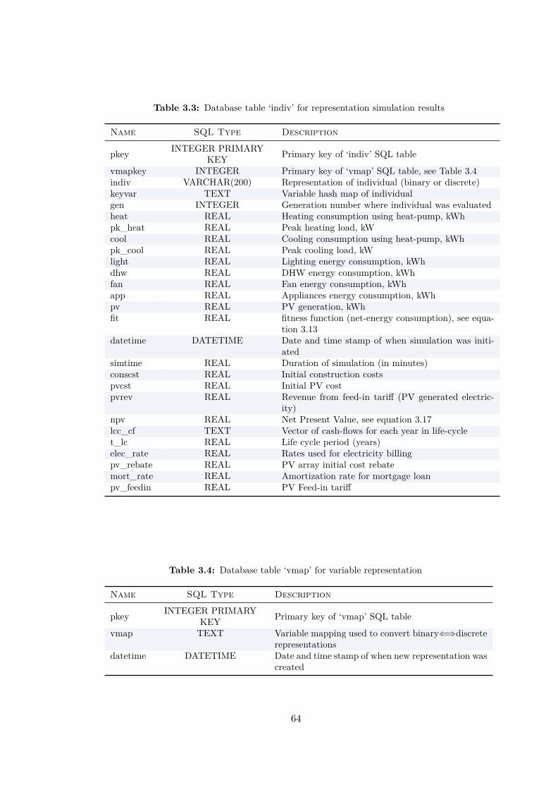
Table 3.3: Database table ‘indiv’ for representation simulation results

Name SQL Type Description

pkey INTEGER PRIMARYKEY Primary key of ‘indiv’ SQL table

vmapkey INTEGER Primary key of ‘vmap’ SQL table, see Table 3.4indiv VARCHAR(200) Representation of individual (binary or discrete)keyvar TEXT Variable hash map of individualgen INTEGER Generation number where individual was evaluatedheat REAL Heating consumption using heat-pump, kWhpk_heat REAL Peak heating load, kWcool REAL Cooling consumption using heat-pump, kWhpk_cool REAL Peak cooling load, kWlight REAL Lighting energy consumption, kWhdhw REAL DHW energy consumption, kWhfan REAL Fan energy consumption, kWhapp REAL Appliances energy consumption, kWhpv REAL PV generation, kWhfit REAL fitness function (net-energy consumption), see equa-

tion 3.13datetime DATETIME Date and time stamp of when simulation was initi-

atedsimtime REAL Duration of simulation (in minutes)conscst REAL Initial construction costspvcst REAL Initial PV costpvrev REAL Revenue from feed-in tariff (PV generated electric-

ity)npv REAL Net Present Value, see equation 3.17lcc_cf TEXT Vector of cash-flows for each year in life-cyclet_lc REAL Life cycle period (years)elec_rate REAL Rates used for electricity billingpv_rebate REAL PV array initial cost rebatemort_rate REAL Amortization rate for mortgage loanpv_feedin REAL PV Feed-in tariff

Table 3.4: Database table ‘vmap’ for variable representation

Name SQL Type Description

pkey INTEGER PRIMARYKEY Primary key of ‘vmap’ SQL table

vmap TEXT Variable mapping used to convert binary⇐⇒discreterepresentations

datetime DATETIME Date and time stamp of when new representation wascreated

64

3.3.7 Multi-Objective Selection Operator

This section discusses the implementation of an additional objective function into an EA.

The multi-objective selection operator determines the formation of the Pareto front. The

inclusion of cost as an objective function, in addition to net-energy consumption, allows

for much more complex interactions between variables. The details of calculating cost

objective functions is discussed in section 3.5. This section discusses EA design modi-

fications to accommodate additional objective functions. This multi-objective selection

operator is later used in Chapter 7.

This section describes the implementation of multiple objectives into a evolutionary

algorithm. However it is not intended to be an exhaustive resource on multi-objective

optimization techniques. For an in-depth analysis, refer to the textbook by Deb (2001)

from which this section is based on.

Multi-objective optimization depends on two concepts: (i) dominance and (ii) Pareto

optimal fronts.

The definition of dominance is described in the following. For a minimization prob-

lem, a vector of decision variables x ∈ X is said to dominate another vector y ∈ X iff

fi(x) ≥ fi(y) for all i = 1, · · · , k and fj(x) > fj(y) for at least one j. If there does

not exist any other decision vector in X that dominates vector x∗, then x∗ is said to be

Pareto optimal.

Dominance allows for comparison of fitness evaluations on individuals using several

objective functions. This concept is necessary as individuals can no longer be compared

using one objective function—comparisons of design alternatives must use all objective

functions. Non-dominated individuals form the optimal solution set indicating that each

individual in the Pareto set has performance characteristics which are unique. This is

a departure from the single objective optimization where one individual dominates all

others.

A population is said to converge if it approaches the Pareto front, see Figure 3.5.

Most multi-objective operators encourage spreading across Pareto fronts using non-

dominated individuals. Crowding distance equations are used to quantify the density

of individuals. Preference is given to individuals which are Pareto optimal and have

the largest spreading relative to other individuals in the population. Spreading of indi-65

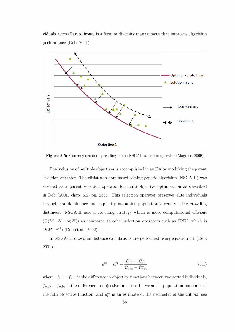
viduals across Pareto fronts is a form of diversity management that improves algorithm

performance (Deb, 2001).

Figure 3.5: Convergence and spreading in the NSGAII selection operator (Magnier, 2009)

The inclusion of multiple objectives is accomplished in an EA by modifying the parent

selection operator. The elitist non-dominated sorting genetic algorithm (NSGA-II) was

selected as a parent selection operator for multi-objective optimization as described

in Deb (2001, chap. 6.2, pg. 233). This selection operator preserves elite individuals

through non-dominance and explicitly maintains population diversity using crowding

distances. NSGA-II uses a crowding strategy which is more computational efficient

(O(M · N · log N)) as compared to other selection operators such as SPEA which is

O(M · N2) (Deb et al., 2002).

In NSGA-II, crowding distance calculations are performed using equation 3.1 (Deb,

2001).

dm = dmi +

fmi−1 − fm

i+1fm

max − fmmin

(3.1)

where: fi−1 −fi+1 is the difference in objective functions between two sorted individuals,

fmax − fmin is the difference in objective functions between the population max/min of

the mth objective function, and dmi is an estimate of the perimeter of the cuboid, see

66

Figure 3.6. The crowding distance of individuals with no neighbours (extrema) is set to

infinity.

Figure 3.6: NSGA-II distance calculation (Deb, 2001)

After crowding distance calculations, individuals are ranked into fronts, and the se-

lection process is conducted, see Figure 3.7. Individuals common to fronts F1 and F2

survive to the next population based on rank. Individuals from front F3 are selected

based on crowding distance to form the remaining population which is used for genetic

operators. Deb (2001) recommended that since the NSGA-II parent selection is deter-

ministic, the survivor selection operator must have some probabilistic characteristics.

Figure 3.7: NSGA-II selection procedure (Deb, 2001)

Multi-objective optimizations require larger population sizes to spread across Pareto

fronts; however early objective function evaluations rarely contribute the identification

of non-dominated individuals. Thus, it is desirable to restrict population sizes and

use over-selection to grow a population of individuals, see Figure 3.8. This innovation

allowed for an identical number of fitness evaluations as the single objective EA by using67

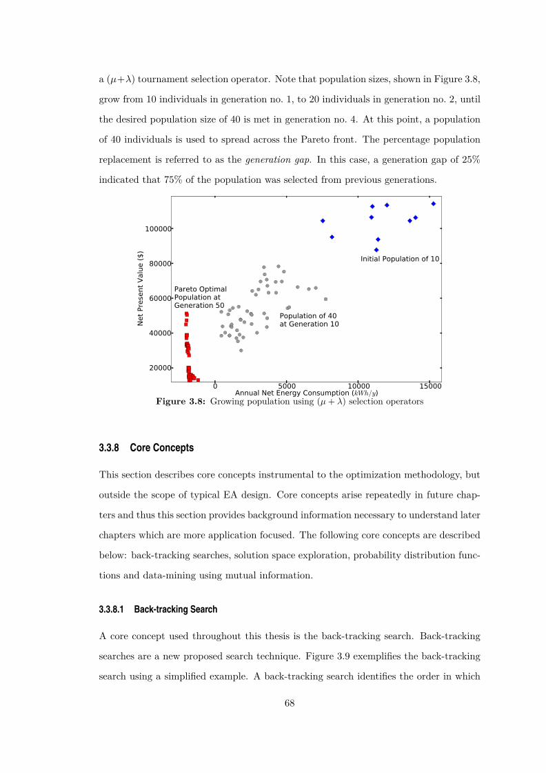
a (μ+λ) tournament selection operator. Note that population sizes, shown in Figure 3.8,

grow from 10 individuals in generation no. 1, to 20 individuals in generation no. 2, until

the desired population size of 40 is met in generation no. 4. At this point, a population

of 40 individuals is used to spread across the Pareto front. The percentage population

replacement is referred to as the generation gap. In this case, a generation gap of 25%

indicated that 75% of the population was selected from previous generations.

0 5000 10000 15000Annual Net Energy Consumption (kWh/y)

20000

40000

60000

80000

100000

NetPresentValue($)

Initial Population of 10

Population of 40at Generation 10

Pareto OptimalPopulation atGeneration 50

Figure 3.8: Growing population using (μ + λ) selection operators

3.3.8 Core Concepts

This section describes core concepts instrumental to the optimization methodology, but

outside the scope of typical EA design. Core concepts arise repeatedly in future chap-

ters and thus this section provides background information necessary to understand later

chapters which are more application focused. The following core concepts are described

below: back-tracking searches, solution space exploration, probability distribution func-

tions and data-mining using mutual information.

3.3.8.1 Back-tracking Search

A core concept used throughout this thesis is the back-tracking search. Back-tracking

searches are a new proposed search technique. Figure 3.9 exemplifies the back-tracking

search using a simplified example. A back-tracking search identifies the order in which

68

each variable should be changed to result in the steepest objective function gradients

from a selected individual, A, to a known reference individual, B. In Figure 3.9, starting

from A three potential variable changes are tested. The variables, x1, x2, x3, are changed

from the value found in the selected individual to the value known in the reference in-

dividual. Thus three new intermediate individuals, C, C1, C2, are created and evaluated

using the objective function. The variable x3 resulted in the steepest change in the ob-

jective evaluation and is identified as the variable with the highest importance as listed

in the x-axis. The objective function gradient from A to C is recorded. Now, the vari-

able x3 can be excluded from the remaining back-tracking searches. Starting from the

intermediate individual, C, the variable x2 with the next steepest gradient is identified

for individual D. This process is repeated until all variables of A are back-tracked to

B. Importance factors, as described in chapter 6, are used to summarize back-tracking

results.

Design of interest to back-trackA=(0.3, 2.0, 40)

Obj

ectiv

e Fu

nctio

n, F

(x1,

x 2,x

3) =

x1+

x 2+x

3 Design Variables:x1: (0.1, 0.2, 0.3, 0.4)

x2: (1.0, 2.0, 3.0, 4.0)

x3: (10, 20, 30, 40)

Arrow of steepest descent:x3: C=(0.3, 2.0, 40 10)

x2: C1=(0.3, 2.0 1.0, 40)

x1: C2=(0.3 0.1, 2.0, 40)

Next arrow of steepest descent:D=(0.3, 2.0 1.0, 10)

x3 x2 x1

Final gradient to Ref. DesignB=(0.3 0.1, 1.0, 10)

Variable Order of Steepest Descent

Figure 3.9: Simplified back-tracking search of vector A back-tracked to reference design vectorB

3.3.8.2 Exploration of Solution Space using Repeated Optimization Runs

Repeated optimization runs are required to use optimization algorithms to extract in-

formation from the solutions space. Consider the solutions space shown in Figure 3.1069

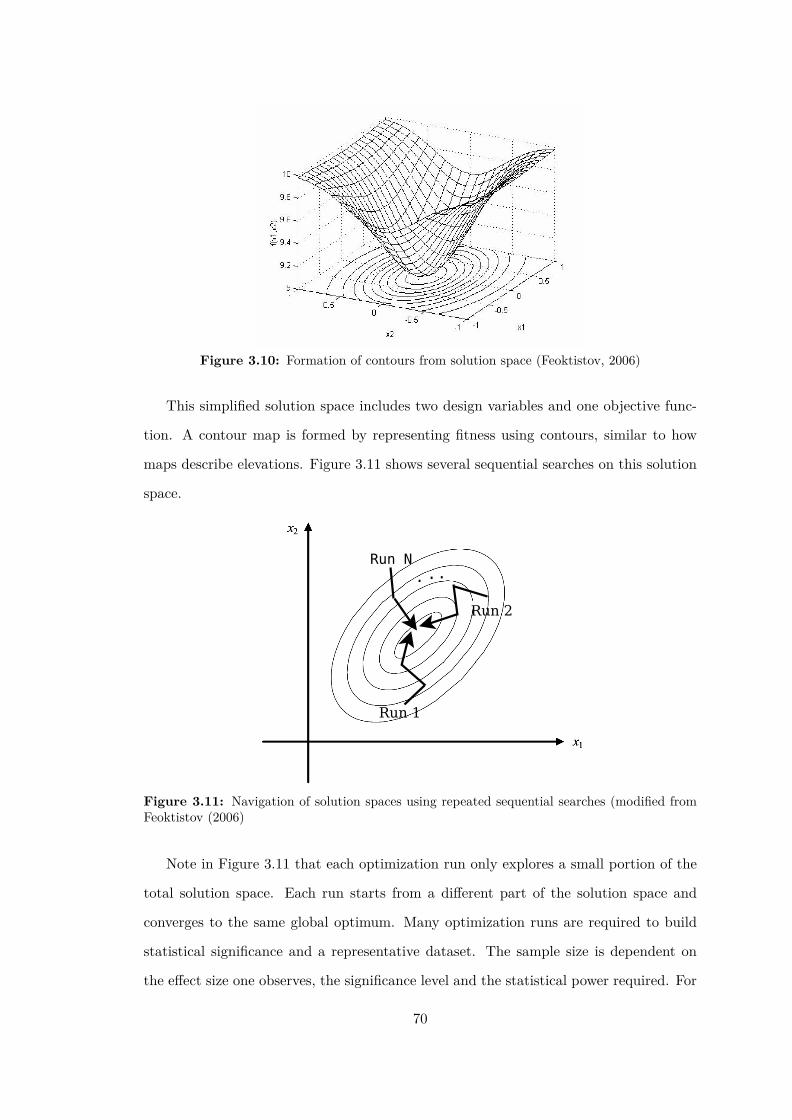
Figure 3.10: Formation of contours from solution space (Feoktistov, 2006)

This simplified solution space includes two design variables and one objective func-

tion. A contour map is formed by representing fitness using contours, similar to how

maps describe elevations. Figure 3.11 shows several sequential searches on this solution

space.

Run 1

Run 2

Run N. ..

Figure 3.11: Navigation of solution spaces using repeated sequential searches (modified fromFeoktistov (2006)

Note in Figure 3.11 that each optimization run only explores a small portion of the

total solution space. Each run starts from a different part of the solution space and

converges to the same global optimum. Many optimization runs are required to build

statistical significance and a representative dataset. The sample size is dependent on

the effect size one observes, the significance level and the statistical power required. For

70

optimization studies of 20 or 30 variables, a sample of 10 to 20 optimization runs is

sufficient depending on the number of algorithm iterations.

3.3.8.3 Probability Distribution Functions

“There are known knowns; there are things we know that we know. There areknown unknowns; that is to say there are things that, we now know we don’tknow. But there are also unknown unknowns—there are things we do not know wedon’t know.

–United States Secretary of Defense, Donald Rumsfeld”In previous sections, the goal of an optimization study was to identify the best per-

forming designs. This section describes a departure from this perspective. Optimization

approaches coupled with visualization tools can aid in identifying trade-offs in the solu-

tion space. This can be accomplished using Probability Distribution Function (PDF).

Recall that the formation of building models relies on many assumptions. Assump-

tions arise from known-unknowns such as occupancy patterns and envelope composi-

tions. However, unknown-unknowns can also arise from overlooked or underestimate

aspects of the simulation process. For example, consider design changes due to budget

restrictions or unavailable materials or equipment. Unknown or uncertain variables can

be included by associating variables to PDFs and simulating all possible scenarios.

Building simulation can be performed using deterministic or probabilistic models,

see Figure 3.12. Traditional deterministic models require all variables to be unique prior

to simulation. Probabilistic models require PDFs to be assigned to input variables. The

probabilistic inputs are sampled to select individual values, then evaluated in the model

to form output distributions. The sampling and analysis to probabilistic input distribu-

tion is referred to as a type of uncertainty analysis called a Monte Carlo simulation.

The following steps are required to form PDFs from optimization data: (i) create

dataset using repeated optimization analysis; (ii) query sets of designs with interesting

characteristics; and (iii) convert query results to PDFs for each variable.

For example, in the following database query, the window frame types variable (FT)

which includes parameters (1, 2) would be associated with a PDF of (45 , 1

5). Stating

this mathematically FT ∈ (1, 2) → (45 , 1

5). Similarly for variable for glazing type GT_s

∈ (3, 4, 5) → (15 , 2

5 , 25). These results can then be exported into a statistical tool such as

R (R Foundation, 2012) for analyses or be converted directly into PDFs for sampling.71

(a) Deterministic Model

(b) Probabilistic Model

Figure 3.12: Deterministic versus probabilistic models (Heo et al., 2011)

1 −− S e l e c t unique v a r i a b l e d e s c r i p t i o n s and f i t n e s s . . .2 −− f o r a l l NZE homes from tab l e ‘ indiv ’ .3 −− Randomly s e l e c t 5 r e p r e s e n t a t i v e de s i gn s .4 −− Round f i t n e s s to one decimal p lace .5 SELECT DISTINCT keyvar ,ROUND( f i t , 1 ) FROM ind iv6 WHERE f i t <0 ORDER BY RANDOM( ) LIMIT 5 ;

Listing 3.1: SQL query for extracting information for probability densities

1 −− KEYVAR | FIT2 { :FT 1 , :GT_n 5 , :GT_s 4 , : a spect 1 . 8 , : a z i −5.6 , . . . } | − 2 0 6 9 . 73 { :FT 1 , :GT_n 5 , :GT_s 3 , : a spect 1 . 1 , : a z i −5.6 , . . . } | − 1 8 1 7 . 74 { :FT 1 , :GT_n 4 , :GT_s 5 , : a spect 1 . 9 , : a z i 0 . 0 , . . . } | − 1 5 9 3 . 85 { :FT 1 , :GT_n 5 , :GT_s 4 , : a spect 1 . 6 , : a z i 16 . 9 , . . . } | − 1 5 3 4 . 66 { :FT 2 , :GT_n 4 , :GT_s 5 , : a spect 2 . 1 , : a z i 16 . 9 , . . . } | − 1 9 9 4 . 6

Listing 3.2: Results from above SQL query

PDFs extracted from optimization results exhibit emergent properties and depend

on the performance of the designs they are extracted from. Some variables might be

monotonic meaning that increasing or decreasing an input variable will always increase or

decrease the outcome. These variables are not interesting in the optimization sense since

72

they behave predictably. However, they are interesting with regards to an uncertainty

analysis. For example, at what variable limit is a performance target no longer met?

What other variables are codependent on a particular variable? Figure 3.13 shows how

PDFs can change with decreasing EUI. In this Figure, note that variable 2 is monotonic

and has a parameter cut-off. Variable 1 shows two probable regions for low EUI and all

parameter combinations are possible.

Energy Use IntensityHighNZE

min max

.

.

.

min maxmin maxmin max

min maxmin max

probprob prob

Low

var 1

var 2

Figure 3.13: Emergent properties of PDFs with EUI reductions

PDFs are used later in chapter 6. Using a completely different approach, in Ap-

pendix A PDFs are specified using normal distribution functions. The goal of this

appendix is to build confidence in economic estimates by conducting an uncertainty and

sensitivity analysis on the cost-model used.

3.3.8.4 Variable Interaction Extraction using Mutual Information

This section describes how mutual information can extract variable interactions. By

definition, mutual information is a measure of dependency between two random vari-

ables (Cover and Tomas, 2006). Due to its Bayesian roots, the updating of mutual

information throughout the optimization search reduces the uncertainty and builds con-

fidence in selected variables interactions.

In communication theory, variable interdependencies are leveraged to shrink the

capacity of the communication channel (Shannon and Weaver, 1947). If the value of one

interdependent variable is known and sent through the channel, then the other variable

can be inferred indirectly. The notion of using predicted variable interactions can be

73

used in an optimization algorithm.

One effective way to extract variable interdependencies is to use the mutual informa-

tion shared between two design variables denoted by I(Xi, Xj) in equation 3.2 (Cover

and Tomas, 2006), noting that xi belongs to the set Xi (xi ∈ Xi) and xj belongs to the

set Xj (xj ∈ Xj).

I(Xi, Xj) =∑

xi,xj

p(xi, xj) · log2

(p(xi, xj)

p(xi) · p(xj)

)(3.2)

Probability calculations are made using representations of previously simulated indi-

viduals. The functions p(xi) and p(xj) are the marginal probability functions of discrete

random variables Xi and Xj for a given performance range. Similarly, p(xi, xj) is the

joint probability for discrete variables Xi and Xj for a specified performance range.

From p(xi, xj), p(xi), and p(xj) the mutual information common to variables Xi and Xj

can be calculated.

If variables Xi and Xj are independent, then p(xi, xj) = p(xi) ·p(xj) and I(Xi, Xj) =

0, indicating that no information is shared. Larger values of I(Xi, Xj) indicates that

more information is shared between variables Xi and Xj . Given these relations, I(Xi, Xj) ≥0.

The following example shows how mutual information is calculated for simplified

simulation results. Consider the simulation results for two design variables framing type

(FT) and glazing type north (GT_n). Note that mutual information calculations for

only two variables are shown for 6 different building designs.1 −− KEYVAR | FIT2 { :FT 1 , :GT_n 5 , : a spect 1 . 8 , : a z i −5.6 , . . . } | − 2 0 6 9 . 73 { :FT 1 , :GT_n 5 , : a spect 1 . 1 , : a z i −5.6 , . . . } | − 1 8 1 7 . 74 { :FT 1 , :GT_n 4 , : a spect 1 . 9 , : a z i 0 . 0 , . . . } | − 1 5 9 3 . 85 { :FT 1 , :GT_n 5 , : a spect 1 . 6 , : a z i 16 . 9 , . . . } | − 1 5 3 4 . 66 { :FT 2 , :GT_n 4 , : a spect 2 . 1 , : a z i 16 . 9 , . . . } | − 1 9 9 4 . 67 { :FT 2 , :GT_n 5 , : a spect 2 . 1 , : a z i 16 . 9 , . . . } | − 1 6 0 0 . 0

Listing 3.3: Results from above SQL query

The marginal probabilities of variables FT and GT_n are p(FT = 1) = 46 , p(FT =

2) = 26 and p(GT_n = 4) = 2

6 , p(GT_n = 5) = 46 . Joint probabilities for these two

variables are calculated as p(FT = 1, GT_n = 4) = 16 , p(FT = 2, GT_n = 4) =

16 , p(FT = 1, GT_s = 5) = 3

6 , p(FT = 2, GT_n = 5) = 16 . The mutual information

shared between these two variables is:74

I(FT, GT_n) = 16 ·log2

( 16

46 · 2

6

)+ 1

6 ·log2

( 16

26 · 2

6

)+ 3

6 ·log2

( 36

46 · 4

6

)+ 1

6 ·log2

( 16

26 · 4

6

)= 0.0441

(3.3)

Finally, equation 3.4 describes the total information that design variable Xi shares

with all other design variables for a given performance range.

Ii =N∑

j=1I(Xi, Xj) where, j = i (3.4)

Note that deterministic searches work best on variables that are loosely coupled

to other variables in the model, that is variables with low shared information. The

identification and strategic searching of weakly interacting variables improves upon one

shortcoming of population-based optimization searches such as EAs.

Information depends on the fitness of the set of design vectors used for the calcula-

tion. For example, in a building simulation problem, information calculated from the

objective space for a set of design vectors which are evaluated in a range of annual en-

ergy consumption of [800, 1200) MJ/m2 would be different than information calculated

from design vectors evaluated within [400, 800) MJ/m2. Mutual information tends to

increase as EUI decreases since building designs with lower energy consumption tend to

have more strongly coupled variables to achieve a given performance levels. As described

in chapter 4, clustering methods exist to better visualize variable interactions.

Mutual information is used later in chapter 5.

3.4 Concept of Design: Energy Model

“Simplify, simplify, simplify—without sacrificing the truth–Richard Feynman ”“With a good model comes discovery, with discovery comes understanding, with

understanding comes control.–K. Still, Crowd Dynamics ”This section highlights important aspects in calculating the energy consumption of a

home in a cold climate. The descriptions in this section are not intended to be exhaus-

tive and cover all topics involved in a cold climate energy model as this is outside the75

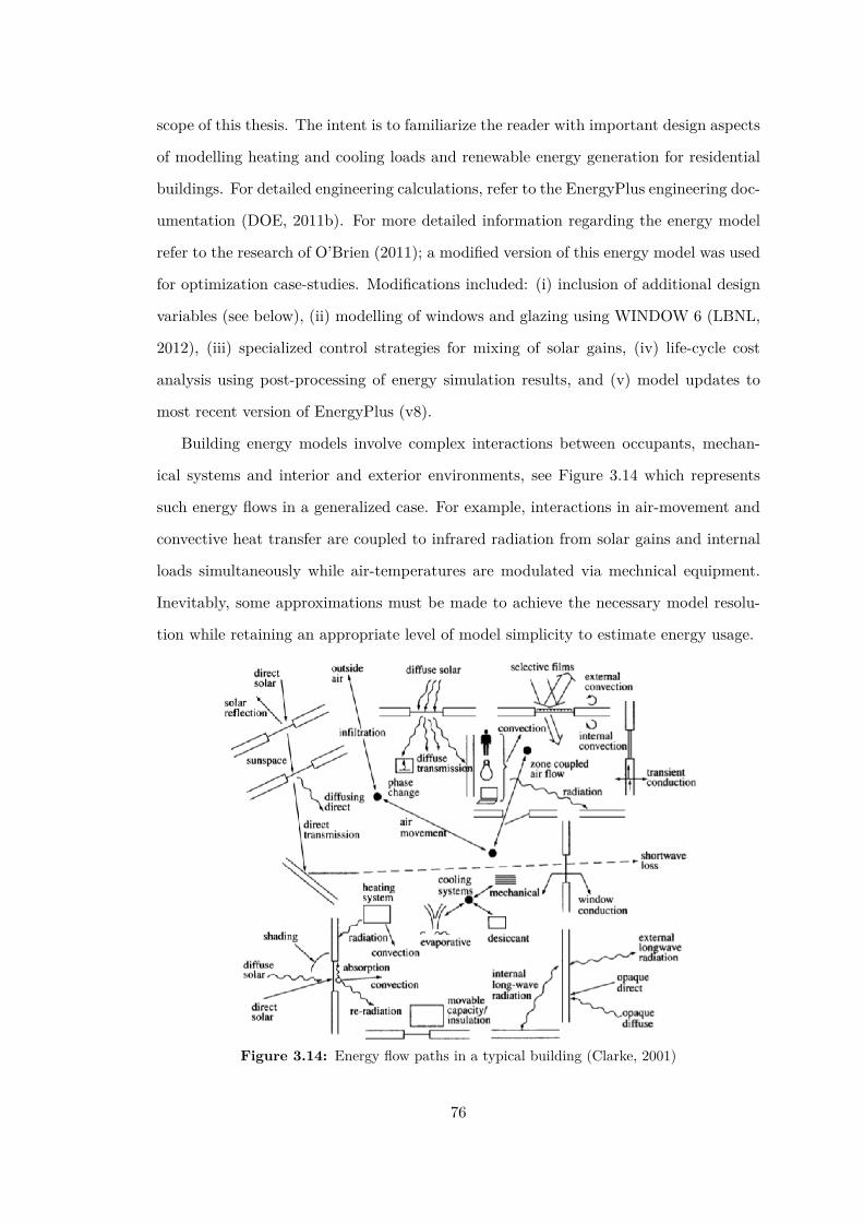
scope of this thesis. The intent is to familiarize the reader with important design aspects

of modelling heating and cooling loads and renewable energy generation for residential

buildings. For detailed engineering calculations, refer to the EnergyPlus engineering doc-

umentation (DOE, 2011b). For more detailed information regarding the energy model

refer to the research of O’Brien (2011); a modified version of this energy model was used

for optimization case-studies. Modifications included: (i) inclusion of additional design

variables (see below), (ii) modelling of windows and glazing using WINDOW 6 (LBNL,

2012), (iii) specialized control strategies for mixing of solar gains, (iv) life-cycle cost

analysis using post-processing of energy simulation results, and (v) model updates to

most recent version of EnergyPlus (v8).

Building energy models involve complex interactions between occupants, mechan-

ical systems and interior and exterior environments, see Figure 3.14 which represents

such energy flows in a generalized case. For example, interactions in air-movement and

convective heat transfer are coupled to infrared radiation from solar gains and internal

loads simultaneously while air-temperatures are modulated via mechnical equipment.

Inevitably, some approximations must be made to achieve the necessary model resolu-

tion while retaining an appropriate level of model simplicity to estimate energy usage.

Figure 3.14: Energy flow paths in a typical building (Clarke, 2001)

76

3.4.1 Energy Balance

EnergyPlus uses a heat balance method to model heat transfer, see equation 3.5 (DOE,

2011b).

CzdTz

dt=

NCL∑i=0

Qi+Nsurf∑

i=0hiAi(Tsi,others−Tz)+

Nzones∑i=0

miCp(Tzi−Tz)+minf Cp(T∞−Tz)+Qsys

(3.5)

where:

CzdTz

dt= Stored energy in zone air

NCL∑i=0

Qi = Sum of Convective Internal Loads

Nsurf∑i=0

hiAi(Tsi,others − Tz) = Sum of heat transferred by convection from zone surfaces

Nzones∑i=0

miCp(Tzi − Tz) = Heat transferred due to interzone mixing

minf Cp(T∞ − Tz) = Heat transferred due to outdoor air infiltration

Qsys = Supplied system load (heating or cooling)

Note: (i) Tz is the zone air temperature; (ii) T∞ is the outdoor air temperature;

(iii) Cz = ρairCpCT is the zone air capacitance; (iv) ρ is the zone air density; (v) Cp

is the zone air specific heat; and (vi) CT is the sensible heat capacity multiplier. The

sensible heat capacity multiplier represents additional thermal mass, such as furniture,

that is equilibrium with the zone air.

Assuming a centralized heating/cooling system and that the zone supply air flow

equals the zone return flow in each zone, the system load is proportional to the difference

of supply air enthalpy and zone temperature, or Qsys = msysCp(Tsupply − Tz).

The building load, Qload is described by the sum of all right hand terms, excluding

the system load. When the capacitance of the air is assumed to be zero, the heat balance

is described by equation 3.5 reduces to Qsys = Qload.

The EnergyPlus solver allows for three potential heat balance algorithms: (i) Euler

method; (ii) analytical solution; and (iii) third-order backward finite difference. The

77

third order backward finite difference method was selected to balance accuracy with

computation time without requiring a prohibitively small time-step.

The derivative term in equation 3.5 can be substituted using a backward finite dif-

ference approximation. Note this could also be formulated using a central or forward

difference in addition to a backward difference (Clarke, 2001).

dT

dt≈ (δt−1)

(T t

z − T t−δtz

)+ O(δt) (3.6)

where: O(δt) is the truncation error; T t−δtz is the node temperature at the previous

time-step.

This first order finite difference model, called the Euler formation, suffers from

higher-order truncation errors for larger time-steps. Taylor et al. (1990) recommended

a third order finite difference method, see equation 3.7.

dTz

dt

∣∣∣∣t

≈ (δt−1)(11

6 T tz − 3T t−δt

z + 32T t−2δt

z − 13T t−3δt

z

)+ O(δt3) (3.7)

where: O(δt3) is the third order truncation error; T t−nδt is the node temperature at the

nth previous time-step. This implicit finite difference method reduces numerical error

by incorporating results from the three previous time-steps.

This equation in combination with equation 3.5 forms the EnergyPlus heat balance

engine.

3.4.1.1 Surface Heat Balance

This section describes the surface heat balance between air-nodes, exterior and inte-

rior surfaces. In EnergyPlus, a first-law heat balance approach ensures that energy is

conserved over each time-step.

The surface heat balance equations require several terms: (i) conduction through a

material; (ii) convection with surfaces and air nodes; (iii) longwave radiant interchange

between surfaces; and (iv) shortwave radiant interchange between surfaces. Longwave

interchanges include radiant exchanges between low-temperature (infrared) objects such

as people, equipment, and other surfaces. Shortwave interchanges include exchanges such

as solar radiation through transparent wall elements and other visible and ultraviolet

78

light sources.

EnergyPlus performs a surface heat balance on the following control volumes: (i) out-

side wall face; (ii) inside wall face; and (iii) inside air heat balance. The heat balances

considered by EnergyPlus are shown below:

qαsol + qLW R + qconv − qko = 0 (Outside Surface Heat Balance)

qLW X + qSW RL + qLW S + qki + qsol + qconv = 0 (Inside Surface Heat Balance)

Qconv + QCE + QIV + Qsys = 0 (Air Node Heat Balance)

where:

qαsol: absorbed beam and diffused solar radiation flux on the exterior wall, W/m2

qLW R: net long-wave radiative flux exchange with the air and exterior environment

(incoming − outgoing), W/m2

qconvo: convective exchange flux with the outside air, W/m2

qko: conductive exchange flux into the wall from the exterior, W/m2. Term is positive

for heat flow into the wall

qki: conductive exchange flux through the wall, W/m2. Term is positive for heat flow

into the wall

qLW X : net long-wave radiative flux exchange between surfaces (incoming − outgoing),

W/m2

qSW RL: net short-wave radiative flux exchange to surfaces from lights, W/m2

qLW S: net long-wave radiative flux from equipment to surfaces in zone, W/m2

qsol: transmitted exterior solar radiative flux absorbed at surfaces, W/m2

Qconvi: convective heat transfer from interior surfaces to the air node, W

QCE: convective portions of internal loads (people, lights and equipment), W

QIV : sensible loads caused by infiltration and ventilation (fresh air into zones), W

79

Qsys : heat transfer to and from HVAC system, W

Figure 3.15 shows the heat balance for the inside surface. The heat balance equation

is coupled to the air-node heat balance through convective terms and the exterior heat

balance equation through the exterior conduction term.

Figure 3.15: Inside surface heat balance diagram (DOE, 2011b)

Long-wave radiation exchanges between zone-surfaces are calculated using simplified

view factors (DOE, 2011b). The calculation requires a matrix of view factor exchange

coefficients for all exchange paths between surfaces. An assumption is made that all

surface radiation properties are grey and all radiation is diffuse. Light introduced into

the zone by mechanical equipment is defined using a radiative/convective split. Once

the view factor coefficients are determined, the long-wave radiant exchange is calculated

for each surface using (DOE, 2011b):

qLW X(i,j) = AiFi,j(T 4i − T 4

j ) (3.8)

where: Ai is the area of surface i; Fi,j is the view factor between surface i and j; and

Ti, Tj is the temperature of surfaces i, j.

The distribution of short-wave radiation consists of beam solar radiation, diffuse

solar radiation, and short-wave radiation from electric lights. EnergyPlus determines the

amount of radiation absorbed by opaque surfaces, glass and shading layers, transmitted

through windows into zones and transmitted back out to the exterior windows. Light

transmitted into the zone is distributed to surfaces within the zone using view factors.80

Material absorptance and reflectance properties determine how much energy is absorbed

and reflected by a given surface. After a single bounce, light is assumed to be diffused

to the zone surfaces.

EnergyPlus allows for the adaptive selection of convection coefficients depending

on the flow regime (Beausoleil-Morrison, 2000). In EnergyPlus, convective terms are

specified using the SurfaceProperty:ConvectionCoefficients object.

The conduction terms are formulated using transfer functions. EnergyPlus calcu-

lates Conduction Transfer Function (CTF) using the state-space method (DOE, 2011b).

CTFs require special consideration if they are to be used for conductive heat transfer

through massive wall elements (Beccali et al., 2005). This thesis uses implicit finite dif-

ference to describe conductive heat transfer through massive elements such as concrete

walls and slabs; CTFs were used to described heat transfer through light-weight ele-

ments. As of EnergyPlus version 7.2, users can specify different heat transfer methods

for each surface.

The CTF term for the inside-face is:

qki(t) = −ZoTsi,θ −nz∑

j=1ZjTsi,θ−jδ + YoTso,θ +

nz∑j=1

YjTso,θ−jδ +nq∑

j=1Φj qki,θ−jδ (3.9)

The outside heat flux relates conductive heat fluxes to current and past exterior

surface temperatures and past heat fluxes

qko(t) = −YoTsi,θ −nz∑

j=1YjTsi,θ−jδ + XoTso,θ +

nz∑j=1

XjTso,θ−jδ +nq∑

j=1Φj qko,θ−jδ (3.10)

where:

Xj: Outside CTF, for surfaces j = 0, · · · , nz

Yj: Outside-Inside CTF, for surfaces j = 0, · · · , nz

Zj: Inside CTF, for surfaces j = 0, · · · , nz

Φj: Inside CTF, for surfaces j = 0, · · · , nz

81

δ: time step

Tsi: Inside-face temperature, ◦C

Tso: Outside-face temperature, ◦C

qki: conductive heat transfer on inside face, W/m2

qko: conductive heat transfer on outside face, W/m2

EnergyPlus uses an integrative, simultaneous solver to calculate heat-balances be-

tween plant, building and systems modules, see Figure 3.16. The integrated solution

manager relies on successive substitution iteration to reconcile energy supplies and de-

mand between plant, building and systems modules. This solver is an evolved version

of previous solvers which only allow unidirectional energy flows between modules such

as DOE-2 (DOE, 2011b). For detailed heat transfer formulation using Fourier partial

differential equations and finite difference refer to Clarke (2001).

Figure 3.16: EnergyPlus Integrated Solution Manager (DOE, 2011b)

3.4.1.2 Sparse Matrix Solutions using Finite Difference

This section describes an alternative method of expressing energy balances using a finite

difference method as used by ESP-r (Clarke, 2001). The purpose of this section is to

exemplify an exploitable characteristic of energy balances in building simulation tools

that can improve optimization algorithm convergence properties. Although EnergyPlus

does not use sparse matrix solvers, the loosely-coupled relationship between heat balance

nodes is equally applicable.

82

The heat balance equations can be solved simultaneously using matrix inversion.

For example, equation 3.11 determines future air-temperatures for a single zone by

multiplying a characteristic matrix to the present air-temperatures, see Figure 3.17.

Aθt+δt = Bθt + C = Z (3.11)

where: θn+1 is the temperature vectors at all nodes in the future time-step, θn is the

temperature vectors of all nodes at the present time-step, A is the future time-step

temperature coefficients, B is the present time-step temperature coefficients, and C are

the boundary conditions for the zone. To solve for future node temperatures requires

inversion, i.e. θn+1 = A−1Z.

Figure 3.17: Matrix formation of future-time coefficients (A) for a single thermal zone, whereAθn+1 = Bθn + C (Clarke, 2001)

The characteristic matrix in equation 3.11 is N by N, where N is the number of

temperature nodes. During a typical annual simulation, over five thousand matrix in-

versions are required for a simple single-zone model using one hour time-step (Clarke,

2001). Often, energy models require tens to hundreds of thermal zones.

83

The inversion of future temperature coefficient matrix is computationally intensive.

However, specialized solvers can simplify the solution scheme since these matrices are

sparsely populated. Sparse matrices are primarily populated with zeros meaning that

nodes are largely loosely-coupled to other nodes; these matrices are more densely popu-

lated on the diagonal than on the upper and lower quadrants. Loosely-coupled systems

are sometimes referred to as being approximately linear. In fact, the only reason that

step-wise solvers work for energy simulation is because the building energy models are

loosely-coupled and approximately linear. Tightly coupled systems typically require

simultaneous solutions. ESP-r uses the sparse-matrix property to simplify numerical

solutions (Clarke, 2001). Several thermal zones and potentially a mechanical system are

partitioned and processed independently, see Figure 3.18.

Figure 3.18: Sparse matrix for systems solution to building heat loss in four zone model (Clarke,2001)

Note, nodes not marked by ‘x’ are zero. Building energy simulation can be viewed

as the solution of interlocking of partitioned matrices. The fact that energy models are

loosely-coupled can also expedite the optimization process. System matrices clearly show

that some heat balance nodes are more tightly coupled than other nodes. This char-

acteristic is later data-mined and exploited by a new proposed optimization approach.

Optimization strategies to solve loosely-couple engineering problems are discussed in

Chapter 5.

84

3.4.2 Energy Objective Function

This section describes the objective function used for energy-consumption optimizations.

The formal goal of an energy-consumption minimization study is to find a design

variable vector, x, such that:

min{f(x)} (3.12)

where: x is the design variable vector x = (x1, x2, · · · , xN )T , in design space X ⊂ RN ;

the objective or fitness function, f(), evaluates set of design variables onto an ‘objective’

vector y = (y1, y2, · · · , yM )T where fi ∈ RM , yi = fi(x), fi : R

N → R1 for i =

1, 2, · · · , M , describes the objective or solution space Y ⊂ RM ; min{f(x)} is subject

to L constraints gi(x) ≤ 0 where i = 1, 2, · · · , L; feasible design vectors set x|gi(x) ≤ 0

form the feasible design space X∗, and corresponding objective vectors set y|x ∈ X∗ form

feasible objective space Y∗; for a minimization problem, a design vector a ∈ X∗ is Pareto

optimum if no design vector b ∈ X∗ exists such that yi(b) ≤ yi(a), i = 1, 2, · · · , M .

The objective is to minimize the net-annual energy consumption of a near net-zero

energy home. The objective function is the annual net-electricity consumption of the

building, see equation 3.13. Sub-hourly time-steps of 15 minutes were used to solve

energy balances in EnergyPlus.

f(x) = Qheat/COPH + Qcool/COPC + Eelec − EP V (3.13)

where: x = (x1, x2, · · · , xN )T is a design variable vector; f(x) is the annual net-

electricity consumption of the building (kWh); COP is the average annual coefficient

of performance of the ground-source heat pump in heating and cooling mode, 3.77 and

2.77 respectively; Q is the annual heating and cooling load of the house (kWh); Eelec is

the gross annual electricity consumption in lighting, appliances and plug-loads (kWh)

and; EP V is the electricity generated by the roof-top PV (kWh). When f(x) < 0 this

implies the net-generation of electricity, or a positive-energy house. Energy consumption

calculations include both sensible and latent loads. Modelling of energy related aspects

of a net-zero energy solar house are discussed in this following section.

85

3.4.3 Energy Model Details

This section provides and overview of influential energy modelling considerations. Influ-

ential design elements were identified partly by design of experiment techniques (Goos

and Jones, 2011) such as significance tests within generalized linear models and partly

from previous studies (Charron, 2007; O’Brien, 2011; Verbeeck, 2007; Wang, 2005).

3.4.3.1 Weather Data

Typical weather data was used for energy simulation purposes since real weather data

for a thirty year period would be computationally prohibitive. Typical weather data is

intended to use typical monthly weather based on measured weather data. EnergyPlus

uses Typical Meteorological Year (TMY) version two weather data (DOE, 2011b). Cana-

dian weather information is provided for 144 locations through the Canadian Weather

Energy and Engineering Data Sets (CWEEDS); CWEEDS weather data contains typi-

cal weather for the period 1974–1993. Weather data was recorded typically on an hourly

basis; EnergyPlus interpolates this information down to sub-hourly time-steps.

In BPS, TMY weather data is intended to calculate building loads during a typical

weather period; TMY data is inappropriate to use for peak mechanical system sizing.

Previous research indicated that building simulation results using TMY data is compa-

rable to using real weather data over a yearly period (Crawley and Huang, 1997). It

was assumed that an oversizing factor of 10% was used to size heat pump equipment to

account for additional capacity during peak weather periods.

3.4.3.2 Occupant Behaviour and Internal Heat Gains

Energy related occupant behaviour is an important, but challenging aspect to incor-

porate into building simulation. Although occupant behaviour is not actually a design

variable, it greatly influences on energy consumption. For example, energy-related oc-

cupant behaviour accounted for 37% of ÉcoTerra’s gross energy consumption (Doiron

et al., 2011).

Monitoring of energy consumption and occupant feedback is an important energy

conservation measure in a NZEH. In the ÉcoTerra house, monitoring identified that

the occupants had installed a 5 kW of electric baseboard heaters in the garage space86

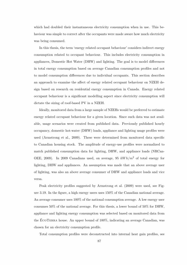
which had doubled their instantaneous electricity consumption when in use. This be-

haviour was simple to correct after the occupants were made aware how much electricity

was being consumed.

In this thesis, the term ‘energy related occupant behaviour’ considers indirect energy

consumption related to occupant behaviour. This includes electricity consumption in

appliances, Domestic Hot Water (DHW) and lighting. The goal is to model differences

in total energy consumption based on average Canadian consumption profiles and not

to model consumption differences due to individual occupants. This section describes

an approach to examine the affect of energy related occupant behaviour on NZEH de-

sign based on research on residential energy consumption in Canada. Energy related

occupant behaviour is a significant modelling aspect since electricity consumption will

dictate the sizing of roof-based PV in a NZEH.

Ideally, monitored data from a large sample of NZEHs would be preferred to estimate

energy related occupant behaviour for a given location. Since such data was not avail-

able, usage scenarios were created from published data. Previously published hourly

occupancy, domestic hot-water (DHW) loads, appliance and lighting usage profiles were

used (Armstrong et al., 2009). These were determined from monitored data specific

to Canadian housing stock. The amplitude of energy-use profiles were normalized to

match published consumption data for lighting, DHW, and appliance loads (NRCan-

OEE, 2009). In 2009 Canadians used, on average, 95 kWh/m2 of total energy for

lighting, DHW and appliances. An assumption was made that an above average user

of lighting, was also an above average consumer of DHW and appliance loads and vice

versa.

Peak electricity profiles suggested by Armstrong et al. (2009) were used, see Fig-

ure 3.19. In the figure, a high energy users uses 150% of the Canadian national average.

An average consumer uses 100% of the national consumption average. A low energy user

consumes 50% of the national average. For this thesis, a lower bound of 50% for DHW,

appliance and lighting energy consumption was selected based on monitored data from

the ÉcoTerra house. An upper bound of 100%, indicating an average Canadian, was

chosen for an electricity consumption profile.

Total consumption profiles were deconstructed into internal heat gain profiles, see

87

Figure 3.19: Peak electricity usage for various user profiles (Armstrong et al., 2009)

Figure 3.20.

Figure 3.20: Breakdown of occupant loads into daily internal gain profiles (O’Brien, 2011)

Phantom loads refer to baseline electricity used for stand-by power in minor and

major appliances, such as electronic devices, wires and appliances. Armstrong et al.

(2009) found the average Canadian home had 65 Watts of standby loss. Occupants were

assumed to generate 120 Watts of heat per occupant. Simulations assumed a family

of four (two parents, two children) occupying the home 50% of the day, see occupancy

schedule in Figure 3.20.

88

3.4.3.3 Building Geometry and Solar Orientation

“In houses that look towards the south [in the northern hemisphere], the sunpenetrates the portico in winter.

–Socrates ”This section describes the interplay between solar orientation and building geometry.

Although Greek philosophers have documented proper solar orientation over 2500 years

ago, interactions between orientation and geometry and other design aspects are still

essential to solar building design today.

In the energy model, rectangular geometries were preferred for optimization studies.

All floor plans were specified using the total floor area and an aspect ratio. From these

two variables, widths and lengths of the building were calculated. In the energy model, a

one or two story floor plan could be specified. Results are relevant to other more complex

geometries if both buildings are thermodynamically equivalent, or have identical direc-

tional heat-loss surfaces, self-shading characteristics and internal air-volumes. Previous

research related to building shape optimization (Wang, 2005) indicated that rectangular

floor plans are comparable to optimal shapes such as pentagonal plans; exotic shapes

such as L-shaped or U-shaped floor plans performed poorly due to their large heat-loss

surface areas compared to other more compact shapes. Furthermore, rectangular shaped

buildings can easily be integrated in to existing grid-based urban environment.

Solar orientation is an important factor in modelling a solar home. Since simula-

tion studies occur in Canada, south-facing implicates orientation towards the sun, or

equatorial-facing. The orientation of the solar home determines the available solar frac-

tion and the peak solar electricity generation using roof-based PV panels. The solar

fraction refers to the percent of heating loads offset using solar gains. Figure 3.21 shows

how orientation affects solar gains and the time of peak temperature gains in a solar

house (Henderson and Roscoe, 2010).

The following sections discuss several envelope modelling considerations for exterior

above-grade walls, below-grade basement walls, basement slabs and the ceiling envelope.

89

Figure 3.21: Relation of azimuth to peak solar gains (Modified from Henderson and Roscoe(2010))

3.4.3.4 Above-grade Walls

This section describes the wall construction used for this thesis, see Figure 3.22. A cold

climate construction consisted of two inches of rigid extruded polystyrene insulation, two

2x4” walls filled with dense-pack cellulose insulation. The advantage of having exterior

rigid insulation is that thermal bridging is eliminated by using a continuous layer of

insulation continued from below the slab, up the basement walls to the ceiling envelope.

A double 2x4" wall was considered for all designs. This wall construction has several

advantages, a double 2x4“ wall: (i) can be insulated to any amount by increasing the

spacing between the two frames; (ii) is simple to air-seal; (iii) is roughly cost equivalent

to a 2x6" wall due to 2x4"s studs being less expensive than 2x6" studs; and (iv) has few

thermal bridges due to use of dense-packed cellulose insulation. Figure 3.23 shows the

framing method used in a double 2x4" wall (courtesy of Habitat Studio).

The following assumptions were made when modelling wall envelopes: (i) a rain-

screen using naturally ventilated exterior brick prevented rain from saturating the wall

envelope; (ii) the envelope was sufficiently air-tight such that moisture in air transport

through the wall cavity into the zone could be ignored from cooling load calculations;

(iii) an interior vapour barrier decoupled the majority of moisture transfer mechanisms;

90

Figure 3.22: Moisture treatment of the wall envelope (Lstiburek, 2009)

Figure 3.23: Construction of a double 2x4" wall (courtesy of Habitat Studio)

91

and (iv) two inches of rigid insulation was sufficient to keep the interior surface of the

rigid foam above the dew-point temperature.

3.4.3.5 Ceiling Envelope

Ceilings heat loss is typically the most significant envelope due to heat stratification in

a multi-story home. Ceiling envelopes require moisture control and attic ventilation to

control potential condensation issues. The following assumptions were made when mod-

elling the ceiling envelope: (i) 3.5 inches of closed-cell polyurethane spray foam provided

air-sealing and decoupled moisture transfer to the attic to the ceiling; (ii) remaining level

achieved using loose-pack blown-in insulation; (iii) eve compression was eliminated using

raised heel trusses, see Figure 3.24; and (iv) attic was ventilated at 6 ACH using baffles

and ridge vents to prevent moisture build-up in the attic space.

(a) Section of Common Roof Truss (b) Section of Raised Roof Truss

Figure 3.24: Section of common and raised roof trusses

The presence of eve-compression in a ceiling envelope, shown in Figure 3.24, results

in greater heat loss near the top of walls than through mid-centre attic sections. Eve-

compression can cause a reduction in the effective insulation value of the ceiling envelope

and moisture damage through ice-damns. Raised heel trusses allowed for a uniform layer

of insulation throughout the attic space.

3.4.3.6 Below-grade Walls

Basement heat-loss is thought to account for 10–40% of total heat-loss in Canadian

housing (Beausoleil-Morrison, 1996). Since basement heat-loss depends on insulation

levels and the presence of thermal bridging, one-dimensional heat-loss calculations do92

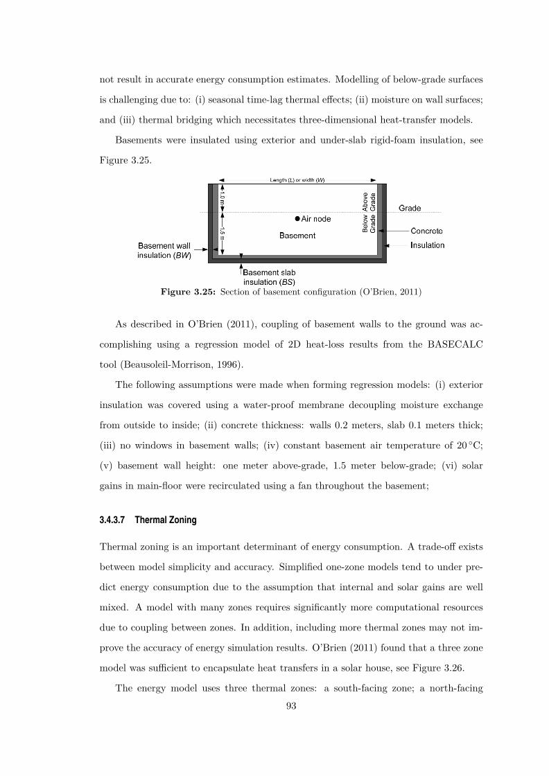
not result in accurate energy consumption estimates. Modelling of below-grade surfaces

is challenging due to: (i) seasonal time-lag thermal effects; (ii) moisture on wall surfaces;

and (iii) thermal bridging which necessitates three-dimensional heat-transfer models.

Basements were insulated using exterior and under-slab rigid-foam insulation, see

Figure 3.25.

Figure 3.25: Section of basement configuration (O’Brien, 2011)

As described in O’Brien (2011), coupling of basement walls to the ground was ac-

complishing using a regression model of 2D heat-loss results from the BASECALC

tool (Beausoleil-Morrison, 1996).

The following assumptions were made when forming regression models: (i) exterior

insulation was covered using a water-proof membrane decoupling moisture exchange

from outside to inside; (ii) concrete thickness: walls 0.2 meters, slab 0.1 meters thick;

(iii) no windows in basement walls; (iv) constant basement air temperature of 20 ◦C;

(v) basement wall height: one meter above-grade, 1.5 meter below-grade; (vi) solar

gains in main-floor were recirculated using a fan throughout the basement;

3.4.3.7 Thermal Zoning

Thermal zoning is an important determinant of energy consumption. A trade-off exists

between model simplicity and accuracy. Simplified one-zone models tend to under pre-

dict energy consumption due to the assumption that internal and solar gains are well

mixed. A model with many zones requires significantly more computational resources

due to coupling between zones. In addition, including more thermal zones may not im-

prove the accuracy of energy simulation results. O’Brien (2011) found that a three zone

model was sufficient to encapsulate heat transfers in a solar house, see Figure 3.26.

The energy model uses three thermal zones: a south-facing zone; a north-facing

93

Figure 3.26: Effect of thermal zoning on electrical energy-consumption (O’Brien, 2011)

zone; and a basement zone. An additional unconditioned roof zone couples roof heat-

gains to the adjacent ceiling. Thermal gains from plug-loads and solar radiation are re-

distributed through conditioned spaces using an air-flow network. A trade-off between

air recirculation and electricity cost for fans was modelled; thus, the recirculation rate

between thermal zones is considered as an optimization variable.

3.4.3.8 Thermal Mass

Thermal mass can reduce peak heating and cooling loads of a solar heated house. Passive

storage of solar gains during periods of peak solar gains acts like a thermal capacitor. An

additional advantage is that surplus solar gains can be stored and discharged during later

periods. This reduces the reliance on mechanical systems for heating. Stated simply,

thermal storage regulates air-temperature fluctuations and can reduce over-heating and

over-cooling. From the perspective of frequency domain analysis, thermal mass acts

as a low-pass filter to moderate high-frequency variations in solar or plug-load heat

gains (Athienitis and Santamouris, 2002).

The primary form of thermal mass is concrete in direct contact with solar gains

through glazing. Warmer floors then reradiate to the surrounding cooling walls and

furniture. It is well documented that a large surface area of thermal mass is more effective

than a concentrate volume (Candanedo, 2011; Charron, 2007; Tzempelikos, 2005). Thus,

94

the energy model just considers thermal mass on concrete floors and on the vertical wall

surface separating the south and north zones. An assumption was made that all floors

were not covered with carpets or flooring. It is well known that the effectiveness of

thermal mass is compromised if covered (Charron, 2007; Chiras, 2002). Concrete floor

and wall thickness was considered as an optimization variable. All concrete was assumed

to have the following properties: (i) conductivity of 1.95 W/mK; (ii) density of 2240

kg/m3; (iii) specific heat of 900 J/kgK; (iv) emissivity of 0.5; (v) reflectance of 0.9; and

(vi) absorptance of 0.7.

A secondary form of mass is the thermal capacitance of air and other massive ob-

jects in the thermal zone such as furniture. The energy model uses an air capacitance

multiplier of 20, see variable CT in equation 3.5, to add additional thermal inertia to

the environment as recommended by the EnergyPlus engineering guide (DOE, 2011b).

Centralized thermal storage in the form of seasonal storage, water cisterns, or ground

storage is outside the scope of this thesis. For further information refer to IEA Annexes

21–26 (IEA, 2013).

3.4.3.9 Comfort Models

This section describes the assumptions made to consider acceptable comfort in energy

simulations.

Popular comfort models, such as the Fanger model (1971), require several unknown

parameters such as metabolic rates, clothing insulation levels as well as known pa-

rameters from simulation such as air-speeds, relative humidity levels and mean-radiant

temperatures. In the Fanger model, comfort is calculated using a predictive mean vote

on a scale from -4 to 4 where 0 is the ‘ideal’ comfort level. This model is static since

occupants cannot interact with their environment to adapt their comfort. Adaptive

comfort models (Nicol and Humphreys, 2002) assume that occupants can modify their

clothing and adapt to seasonal temperatures. These models are appropriate for residen-

tial environments or office environments where individualized environmental control is

provided. Adaptive models were not considered since they require additional uncertain

information to make comfort calculations and thus were outside the scope of this thesis.

There is on-going debate about whether comfort should be considered an optimiza-

95

tion criterion or as an optimization constraint. One perspective argues that comfort

is quantifiable in early simulations and a given design can be more comfortable than

another, so comfort is an added objective function in a optimization study. The other

perspective is that comfort models are too uncertain since they depend on hourly values

of temperature, air velocity, relative humidity, intra-zone mixing and occupant clothing

levels, all variables which are difficult to predict over an annual period.

Perhaps comfort is better handled as an optimization constraint and that mechan-

ical systems should be sized to ensure that heating and cooling setpoints are satisfied

throughout the simulation period. The automatic sizing of mechanical systems to meet

setpoints under peak seasonal conditions actively constrains air-temperatures to an ac-

ceptable level. Thus, comfort in this thesis is not considered directly but indirectly using

zone air-temperatures modulated by HVAC systems. This approach has the following

advantages: (i) all designs considered have acceptable air temperature throughout the

simulation period but may require larger HVAC systems; and (ii) the relationship be-

tween energy consumption and air-temperature setpoints can be examined. The detailed

simulation of models which do not achieve acceptable set-point schedules is considered

a waste of computational resources. Active constraining of comfort enables the data-

mining of all previous simulations to identify interesting design features. If comfort

was considered as an objective function, only a subset of simulations would be usable

for data-mining. This approach assumes that occupants will adapt clothing levels or

metabolic activities to air temperature setpoints.

The heating and cooling needs are determined via a setpoint schedule. Models used

nightly setback schedules during the evening (10pm–7am). Cooling systems were en-

abled from May to September. The lower and upper temperature setpoints define the

temperature dead-band, i.e. the range of temperature were no heating or cooling inter-

ventions are required, see Figure 3.27.

The temperature dead-band is a major determinant of energy consumption and occu-

pant comfort. If the dead-band is narrow, then an over-reliance on short-cycling of me-

chanical systems is required to satisfy temperature schedules and charge passive thermal

storage. As shown in Figure 3.27, a wide dead-band allows for free-floating conditions

but at the risk of occupant discomfort. As previously mentioned, the implementation of

96

Figure 3.27: Temperature dead-band from monitored data in the ÉcoTerra solar home(Modified from Doiron (2010))

thermal comfort models in the energy methodology is outside the scope of this thesis.

Comfort is considered indirectly by controlling mean radiant air-temperatures.

3.4.3.10 Window, Overhangs and Blind models

This section describes modelling details related to window, blinds and overhangs. The

combination of these three technologies determines the utilization of impinging, useful

solar radiation on the transparent facade. A solar optimized house uses solar gains

during the heating seasons to offset heating loads and protects the interior from over-

heating during the cooling season. The WWR is defined as the area of glazing and

framing relative to the total facade areas for each directional wall surface.

window 6 was used to specify glazing properties (LBNL, 2012). EnergyPlus can

use window 6 results to specify several important window system properties such as:

(i) average window-frame heat transfer properties from 2D calculations; (ii) inside and

outside projection distances; (iii) conduction and optical properties due to different gas

mixes (up to three gases); (iv) hemispherical emissivity properties for each pane; (v) edge

conduction properties; and (vi) glazing optical properties for different incident angles

and solar spectrum wavelengths.

97

Table 3.5 describes window types available in the energy model. In EnergyPlus,

windows are defined by construction layers and the optical properties of the glazing

unit. Two window framing types, wood and vinyl could be specified as optimization

variables (wood denoted by 1, vinyl by 2). Window sizing was calculated from facade

area and the WWR fraction. Windows were grouped into a single window object for

each wall surface. Note windows were not modelled in the basement zone.

Table 3.5: Window properties used in energy model (O’Brien, 2011)

Roller shading with visible spectrum reflectance of 0.8, emissivity of 0.9 and conduc-

tivity of 0.3 W/m2K were used. Roller shades were automatically deployed if exterior

solar radiation on the exterior window surface exceeded 150 W/m2 and if exterior tem-

perature on the window exceeded 20 ◦C. These values ensured that blinds were closed if

there was potential for zone overheating. This was determined via a previous simulation

study (O’Brien, 2011).

Depending on the orientation of the main solar collecting surface, glazings could

account for a net-heat gain over the heating season. This indicates that more solar

radiation is gained over the simulation period than lost due to heat transfer. Fig-

ure 3.28 (O’Brien, 2011) shows all double and triple glazed windows described in Ta-

ble 3.5 have net-solar gains if oriented south.

Exterior shading prevents unwanted solar gains during the cooling season. Deploy-

able canvas window awnings provided shading for south facing windows, see Figure 3.29.

The overhang distance was calculated using maximum and minimum solar angles or98

Figure 3.28: Heat-gain for various window types during heating season (O’Brien, 2011)

within the optimization algorithm. Charron (2007); Wang (2005) commented that over-

hangs on east and west-facing facades provided minimal utility due to low solar angles,

and thus were ignored.

Figure 3.29: Window awning

3.4.3.11 Infiltration and Exfiltration

Infiltration is the rate at which air is exchanged between the inside of a building en-

closure and the outdoors. In northern climates, air-tightness is a strong indicator of99

how much energy a building will consume, especially during peak heating and cooling

seasons. One air-change per hour indicates that the air volume in a building is replenish

with fresh outdoor air every hour. Uncontrolled air flow during peak heating season

can significantly increase heating loads. The adage of home builders is to ‘build tight,

ventilate right’ encouraging builders to build as air-tight as possible and use mechanical

equipment to control air into the building.

Infiltration is most commonly measured after post-construction using a blower-door

test. To calculate air-tightness, one must calculate the air-volume of the building,

then measure the air-flow entering the building at various air-pressures. It is rec-

ommended that infiltration be measured by both pressurizing and depressurizing the

building (ASHRAE, 2011a), see Figure 3.30 (Krarti, 2011). With this information the

equivalent leakage area, infiltration at 50 Pa and natural infiltration can be calculated.

Figure 3.30: Blower door setup (Krarti, 2011)

Figure C.2, Appendix C, shows blower door measurements for 180,000 homes in

Canada; this data was provided by Natural Resources Canada (NRCan) and collected

through the ecoEnergy programme (NRCan, 2012). The most probable infiltration mea-

surement in this dataset was 3.5 Air Changes per Hour (ACH) at 50 Pa. The tightest

home in this dataset had an air-tightness of 0.48 ACH at 50 Pa. These values determined

the limits of air-tightness in the energy model.

One accurate infiltration method supported by EnergyPlus is the AIM-2 (Walker

and Wilson, 1998) model to calculate infiltration for a given exterior wind speed and

weather conditions using an assumed or measured air-flow rate (DOE, 2011b).

100

Inter-zonal air mixing was considered using a design variable, zone_mix. It was

possible to recirculate air between thermal zones using a fan. However, the fan con-

sumed electricity proportional to the cube of the fan speed. This lead to an interesting

interaction which allowed the energy model to effectively behave like a single thermal

zone if a sufficient amount of electricity was consumed for air recirculation.

Exfiltration refers to the intentional introduction of fresh air for ventilation purposes.

Fresh air can be provided by depressurizing the building using bathroom and kitchen

fans or control exhaust through heat-exchange process in a heat-recovery ventilator.

ASHRAE 62.2 standard (ASHRAE, 2011a) for residential ventilation requires: (i) 8

L/s per person; (ii) additional 0.1 L/s per square foot of floor area; (iii) CO2 concentra-

tion in indoor air do not exceed 700ppm; and (iv) satisfies 80% or more people. Federal

programs in Canada simplified this requirement to 0.3 ACH including mechanical and

natural sources of air during occupied periods (NRCan, 2012). This requirement was

imposed during energy simulations. This requirement allows for some buildings not

to have ventilation equipment if they are not air-tight; very air-tight buildings require

HRVs to satisfy fresh air requirements. An HRV with an efficiency of 60% was used to

provide 0.3 ACH of fresh air during occupied periods.

3.4.3.12 Renewable Energy Generation using Photovoltaic Panels

“If each energy quantum of the exciting light releases its energy independentlyfrom all others to the electrons, the distribution of velocities of the electrons,which means the quality of the generated cathode radiation, will be independent ofthe intensity of the exciting light; the number of electrons that exits the body, onthe other hand, will, in otherwise equal circumstances, be proportional to theintensity of the exciting light.

–Albert Einstein on the Photoelectric Effect (1905)”Electrical generation via PV panels was the primary source of renewable energy. Ad-

vantages of PV panels include: (i) rapidly decreasing costs due to a surplus international

supplies and streaming-lined manufacturing; (ii) electricity has more applications than

process heat from solar thermal; and (iii) electricity can be stored and grid-distributed.

Photovoltaic panels use the photoelectric effect (Einstein, 1905) to generate electric-

ity. The photoelectric effect is a quantum phenomena where an absorbed photon in a

material frees a photo-electron. Photons can only be absorbed if their energy exceeds the

101

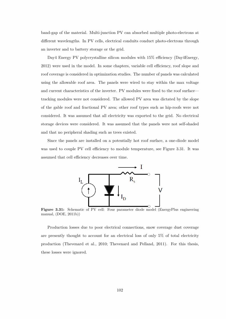
band-gap of the material. Multi-junction PV can absorbed multiple photo-electrons at

different wavelengths. In PV cells, electrical conduits conduct photo-electrons through

an inverter and to battery storage or the grid.

Day4 Energy PV polycrystalline silicon modules with 15% efficiency (Day4Energy,

2012) were used in the model. In some chapters, variable cell efficiency, roof slope and

roof coverage is considered in optimization studies. The number of panels was calculated

using the allowable roof area. The panels were wired to stay within the max voltage

and current characteristics of the inverter. PV modules were fixed to the roof surface—

tracking modules were not considered. The allowed PV area was dictated by the slope

of the gable roof and fractional PV area; other roof types such as hip-roofs were not

considered. It was assumed that all electricity was exported to the grid. No electrical

storage devices were considered. It was assumed that the panels were not self-shaded

and that no peripheral shading such as trees existed.

Since the panels are installed on a potentially hot roof surface, a one-diode model

was used to couple PV cell efficiency to module temperature, see Figure 3.31. It was

assumed that cell efficiency decreases over time.

Figure 3.31: Schematic of PV cell: Four parameter diode model (EnergyPlus engineeringmanual, (DOE, 2011b))

Production losses due to poor electrical connections, snow coverage dust coverage

are presently thought to account for an electrical loss of only 5% of total electricity

production (Thevenard et al., 2010; Thevenard and Pelland, 2011). For this thesis,

these losses were ignored.

102

3.5 Concept of Design: Cost Model

Cost is a primary factor in the economic viability of any new technology, especially

capital intensive project such as building design. Including initial and operating costs

as an additional objective function in NZEH performance evaluations results in a more

complex and non-intuitive solution space. Navigating this problem space using trial and

error simulation strategies is burdensome. In fact, previous researchers attempting to

do so have commented that as many as 10,000 building simulations using parametric

runs was insufficient to find the optimal design (Wright and Farmani, 2001). However,

the exploration of such multi-objective optimization problems could be achieved using

an algorithmic approach such as an EA.

This section describes the cost objective function used to determine a proposed

designs cost effectiveness. The primary source for material and labour costs is the most

recent RSMeans cost catalogue for residential construction (RSMeans, 2013). The cost

analysis presented in this section is an incremental cost analysis. This means that costs

are only considered valid with respect to a reference building, such as the reference

building described in chapter 7. Considering incremental costs relative to a reference

building greatly simplifies the life-cycle analysis, see Appendix C. Detailed costing is

not required for all aspect if they are identical in the actual and reference building.

For example, land acquisition, building inspection and excavation costs can be ignored.

One disadvantage of this approach is that the life-cycle cost of the actual building is

valid only if compared to a particular reference building. An uncertainty and sensitivity

analysis of the cost model is conducted in Appendix A.

3.5.1 Cost Calculation Procedures

ASHRAE (2011c) recommends that economic evaluations be performed with in a life-

cycle analysis. A detailed LCC analysis involves the following terms (Doty and Turner,

2012):

LCCNP V = CNP V + O&MNP V + ENP V − SNP V − INP V (3.14)

where: CNP V : represents capital costs of materials; O&MNP V : is non-energy related

103

operations, maintenance and replacement costs; ENP V : represents operational energy

costs; SNP V : is the salvage or residual value; INP V : is the income generated through

incentives such as feed-in tariffs.

The Net-Present Value (NPV) of each term is calculated using (Doty and Turner,

2012):

NPV =N∑

t=0

Ct

(1 + a)t(3.15)

where: Ct: Net-cash flow at time, t (Net meaning Ct = cashout − cashin); a: is the

minimal acceptable rate of return; and N : number of years considered in the life-cycle

(t=0 is the present year).

If NPV = 0, the investment is considered to be cost neutral over the considered

life-cycle. For this thesis, NPV < 0 is considered to be a profitable opportunity, and

if NPV > 0, the investment is considered to unprofitable over the evaluated life-cycle

period. The transition between non-profitable and cost neutral deserves a special cost-

metric, called the internal rate of return, which is discussed in greater detail later. The

goal of the cost optimization study is to minimize NPV . The goal of a multi-objective

analysis is to minimize net-energy consumption and life-cycle cost using Pareto fronts.

NPV transforms future cash flow into present value using an minimal acceptable

rate of return (MARR) or an expected Return on Investment (ROI). This term is often

referred to as the discount rate. Real and nominal discount rates were used in life-cycle

analyses. Real discount rates represent the loss of money value due to inflation. Nominal

discount rates represent the investor opportunity costs which could be achievable using

other investment vehicles. Nominal discounts rates include inflationary terms. Investors

expect a MARR of 8–12% depending on the risks involved.

To compare a potential investments, economists use guaranteed investment options

such as bank rates, government bonds or Guaranteed Investment Certificates (GIC) to

determine the MARR. The MARR is calculated from equation 3.16 (Doty and Turner,

2012):

a = (1 + r)(1 + i) − 1 (3.16)

where: r is assumed bank rate, 2.14% a return from a 10 year GIC from 2002 to

104

2012 (Bank of Canada, 2009); i is the annual inflation rate, 2.0% in Canada (Bank

of Canada, 2009); a is the minimal acceptable rate of return, 4.18%.

A detailed cost analysis is not possible at the conceptual design stage due to missing

or uncertain information. Thus, some of the terms as described in equation 3.14 are

simplified or ignored based on the criteria outlined below:

• Only material and labour are considered in capital costs. Cost associated with

design or consulting fees, land acquisition and development are not considered. It

is assumed that the appreciation/depreciation of non-design aspects are similar for

all design alternatives.

• Salvage or residual values are considered. Residual values are not used in the sense

that all building materials are to be re-sold. They are used as a method to allow

for variable life-cycle periods. Including salvage values allow for the comparison

of life-cycle periods where some, or all, materials have just been replaced with a

life-cycle period where materials are due for replacement in the following year. It is

assumed that material salvage values depreciate linearly from the initial purchase

until the year of replacement.

• Cost items unaffected by design variables are excluded because they are equal

values for all design alternatives.

• Replacement costs are only considered if they fall within the specified life-cycle.

Capital cost are assume to grow with inflation. Reductions in costs due to expe-

rience curves and improved manufacturing are not considered.

• Non-energy operation and maintenance costs, such as painting, servicing, etc., are

not considered.

• Soft costs, or penalty functions, related to comfort (visual and thermal) are ex-

cluded due to their difficulty to quantify.

In previous research, soft costs or penalty functions penalized designs with visual or

thermal occupant discomfort (Charron, 2007). This approach steers the optimization

algorithm away from solution landscapes which lead to undesirable performance criteria.

105

A disadvantage is that the determination of penalty functions is subjective and may not

be all appropriate for all occupants. To avoid this, active constraints were used in

the optimization algorithm to ensure potential design which do not satisfy temperature

setpoints or work-plane illuminance criteria are not considered.

Based on the aforementioned assumptions, the life-cycle cost equation used for the

analysis is reduced to equation 3.17.

LCCNP V = CNP V + ENP V + RNP V − SNP V − INP V (3.17)

where: CNP V : represents capital costs; ENP V : represents operational energy costs;

RNP V : is replacement costs; SNP V : is the salvage or residual value using linear

depreciation; and INP V : is the income generated through incentives such as feed-in

tariffs.

3.5.2 Life-Cycle Period

Few standards suggest an appropriate evaluation period for a life-cycle cost analysis.

For case-studies, a period of 30 years is considered, although longer period may be used

to project the payback period for building upgrades. European standards, such as EN

15459: Energy performance of buildings—economic evaluation procedure for energy sys-

tems in buildings (2010) does not recommend life-cycle periods greater than 30. Beyond

a 30 year horizon, estimation of interest rates and energy escalation indexes become

near impossible to estimate. Note that the selection of a life-cycle period will affect

the replacement costs of some materials. The use of salvage values allows for variable

life-cycle periods.

3.5.3 Salvage Values

Including replacement costs creates a potential problem: the possibility that costs are

incurred just before the end of the life-cycle results in an artificially high NPV. Thus,

some salvage values need to be associated with each material. This is especially impor-

tant for equipment, such as PV panels and inverters, where costs can vary significantly

from design to design depending on the array size.

106

Salvage values were incorporated using a linear depreciation method, see Figure 3.32.

Initial Cost

Time (year)

Cost ($)

0

Replacement Cost

1 2N

. . .

. . .

Salvage Value (year n)

Figure 3.32: Salvage values: Linear depreciation of initial and replacement costs

It was assumed that materials depreciate linearly over-time until replacement is

required. Thus, at the end of the specified life-cycle period, it is assumed that the

materials purchased have some residual value. In some instances this can be related to

a real resale value, such as PV panels, whereas in other instances, such as insulation

replacement, salvage values are strictly used to compare different life-cycle periods. Note

that other depreciation methods are also available (Doty and Turner, 2012).

Specification of initial and replacement costs are discussed in the following sections.

3.5.4 Material Initial and Replacement Costs

Initial costs were broken down as follows:

C = wallinsCost + ceilinsCost + baseinsCost + slabinsCost + roofCost +

overhangCost + concrCost + PVCost + winCost + airtightCost (3.18)

Each of these capital costs is described in the following sections.

3.5.4.1 Envelope and Insulation Costs

This section describes pricing of exposed wall, ceiling, slab and basement envelopes.

The wall envelope was constructed using a double 2x4" wall with 2" of exterior rigid

closed cell extruded polystyrene, 25 PSI compressive strength insulation board. Exterior107

rigid insulation reduces thermal bridging and improves envelope tightness. Blown-in

cellulose filled in the cavity in the double 2x4" wall. The incremental framing costs

associated with insulating double 2x4" walls was assumed zero since spacing could be

modified to allow for any wall insulation value.

The costs associated with the construction of a wall section is given by equation 3.19.

wallinsCost = wallArea · wallUnitCost (3.19)

Wall areas are calculated based on the specified WWR; thus, trade-offs between

collection of solar energy versus reductions in heat loss using better insulated walls is

embodied in the analysis. A breakdown of wall constructions cost is shown in Table 3.6.

Cellulose insulation in the wall cavities was also scheduled for replacement every 25

years. It was assumed that cellulose required replacement due to material compression

and deterioration.

Table 3.6: Incremental costing data for wall construction

Description thickness(in)

Resistance(R-val/in)

IncrementalCost

($/(in · m2) WA)Extruded polystyrene rigidinsulation

2.0 5.0 8.88

Dense pack cellulose in dou-ble 2x4 staggered framedwall

x ≥ 3 3.6 1.20

The ceiling attached to the attic space was insulated using a mix of closed cell

polyurethane over 2x4" rafters and loose-pack blown-in cellulose. Truss heels were as-

sumed to be raised to reduce additional heat loss through eve-compression. Table 3.7

summarizes ceiling insulation costs. Cellulose attic insulation was scheduled for replace-

ment every 25 years.

Table 3.7: Incremental costing data for ceiling construction

Description thickness(in)

Resistance(R-val/in)

Cost ($/(inft2)FA)

Sprayed polyurethane insu-lation (closed cell) on 2x4rafters

3.5 5.0 7.10

Loose blown-in cellulose in-sulation

x > 7 3.4 1.20

108

Foundation walls were a concrete structure—insulation was accomplished using a

closed-cell polyurethane foam on a 2x4" wall of various distance from the concrete wall

to reach the desired insulation level. A cost of $7.10/m2/in for spray foam was sourced

from RSMeans 2011 data. It is assumed that basement walls are finished in the reference

and upgrade cases, so costing related to drywall and framing can be ignored.

Slab insulation was used to deter heat-loss through the ground and footings of the

basement. Rigid extruded polystyrene insulation was assumed to be place under the

slab at varying thicknesses. RSMeans 2011 data suggested a cost of $8.88/m2/in.

3.5.4.2 Passive Thermal Storage using Concrete

As previously mentioned, concrete slabs and a single vertical concrete wall was used to

passively store solar gains.

Costs were determined for both the concrete floors and wall using RSMeans 2011

data. Table 3.8 shows the cost per concrete thickness.

Table 3.8: Costing data for concrete floor and wall construction

Description Total ($/cm/m2 FA)Concrete Floor, mesh reinforcing, with labour 2.28Concrete Wall, light reinforcing, with labour 5.89

The combined cost for all poured concrete is shown in equation 3.20.

concCost = Afloor · floorUnitCost · dfloor · Nfloor +

Awall · conWallUnitCost · dwall (3.20)

where: Nfloor is the number of stories; dfloor is the thickness of the floor; dwall is the

thickness of the wall.

3.5.4.3 Window Costs

Window costs were calculated based on the WWR ratio and the total wall area, see

equation 3.21.winCost = WWR · facadeArea · winUnitCost (3.21)

The window cost data was sourced from RSMean 2011 data, see Table 3.9.

109

Table 3.9: Window costing data

Description Total($/m2)

2-pane, 12.7mm air cavity 477.902-pane, 12.7mm argon cavity, low-e 520.533-pane, 12.7mm air cavity 565.743-pane, 12.7mm argon cavity, low-e 585.74

3.5.4.4 Roofing and Overhang Costs

Roofing and overhangs costing is presented in this section. Recall, that PV is mounted

directly on the roof-top surface. Since there is potential for partial coverage of roof area

using PV, shingles were used to cover the remaining roof area. The unit cost for shingling

from RSMeans 2011 is $37.36/m2 for labour and material. This includes a water-proof

ice-guard membrane for an underlay. Gable roofs were specified to maximize the area

for PV panels. Other roof styles, such as hip roofs were not considered.

Various roof slopes were consider in the cost analysis, see Table 3.10. This created

an interaction between PV-based energy production and material costs. A steeper roof

allowed for a larger area of PV panels and the opportunity for revenue through feed-in

tariffs programs but at the expense of higher roof framing costs and investment into PV

panels.

Table 3.10: Costing data for gable roofs at various pitches

Roof Pitch Roof Slope (◦) Roof Cost ($/m2

FA)3-12 14 79.646-12 27 84.379-12 37 91.4812-12 45 100.4215-12 51 110.6418-12 56 121.62

Canvas window awnings provided shading for south facing windows. Costing data,

sourced from RSMeans 2011, depended on the width of the window requiring coverage.

Each linear foot of window awning was assumed to cost $22 for materials and labour.

Since the protruding distance of the awning is adjustable, this cost is independent of the

awning depth.

110

3.5.4.5 Air-Tightness Costing

Air-tightness cost is difficult to quantify since it depends on the experience and talent of

the builder. Additional costs should lead to a more air-tight house due to better material

selection and a more meticulous installation process. RSMeans has yet to quantify added

costs associated with improving a homes air-tightness. Particularly, we are interested in

additional costs to achieve R2000 air-tightness (1.5ACH@50Pa) down to PassiveHaus

air-tightness standards (0.6ACH@50Pa).

In a conversation with the director of Habitat Studio a designer and builder of several

NZEHs in Canada, and a participant in the Net-Zero Energy Home Coalition (NZEH

Coalition, 2012), the following details were shared. Getting to 3ACH should be possible

without any special materials or additional labour. Achieving an air-tightness of 1.5ACH

requires an additional $3200 of labour and material costs for a 2500 ft2 home. Achieving

PassiveHaus air-tightness standards requires specialized air-sealing products originating

from European markets but is possible for an additional cost of $4000 of labour and

material costs for a 2500 ft2 home. These costs are normalized by the square footage

to arrive at Table 3.11.

Table 3.11: Envelope air-tightness: combined labour and material costsAir-tightness

(ACH at 50 P a)Incremental Cost

($/m2 FA)>3.0 0.0001.5 13.7730.6 17.216

3.5.4.6 Photovoltaic Costing

“We need to invest dramatically in green energy, making solar panels so cheapthat everybody wants them. Nobody wanted to buy a computer in 1950, but oncethey got cheap, everyone bought them.

–Bjorn Lomborg ”As previously mentioned, a PV array was integrated into the building roof-top. It is

assumed that some combination of PV panels and wiring configurations exist to fill any

roof area. Thus the design of PV strings, inverter sizing, etc. is abstracted away from

this cost analysis. A breakdown of costs for a 10kW PV array, see Figure 3.33, is shown

in Table 3.12.

111

Figure 3.33: Diagram of 10kW grid connected PV system (RSMeans, 2012)

Note that although PV module prices have decreased to almost $1/W, modules

account for less than half of the total installation price of a 10 kW PV system shown in

Table 3.12. The material and labour costs associated in safely connecting a grid-tied PV

system also need to be considered in a life-cycle cost-analysis. These miscellaneous costs

were determined to be 3.43 $/W . The cost per watt for a PV panel base case analysis was

$1.50, however, scenarios were considered with PV panel less than this value. Inverters

were intentionally oversized by 20%, a common practice to ensure inverters are never

overloaded.

It was assumed that PV panels were replaced after 40 years and that the inverter

was replaced every 15 years, see Figure 3.34. Chow et al. (2003) suggested that cell

efficiency decreases by 0.1% per year; this was used to model decreasing PV electricity

production over the life-cycle.

Time (year)

Cash Flow ($)

0 1 2

. . .

PV systemcost

Inverterreplacement

15 30

PV systemsalvagevalue

Revenuefrom tari

20Tari Ends

Figure 3.34: Example PV system life-cycle: Feed-in tariff and salvage value

112

Table 3.12: Material and labour costs for a 10kW grid connected PV system (RSMeans, 2012)Description Quanity Unit Material ($) Labour ($) Total ($)PV modules, 167 Watt, 23.5 V 60 Ea 42300 4620 46920Mounting Frames, 6 modules 10 Ea 9650 1250 10900Steel Angle Support 400.0 LF 184 5696 5880# 12 wire 4.0 CLF 146 224 370AC Disconnect switch, 60 A 1 Ea 595 280 875Fuse, 75 A 3 Ea 75 46.20 121.204/0 wire 2.0 CLF 930 432 1362Module Connector 4/0 4 Ea 40.20 352 392.20Combiner box 10 lug, NEMA 3R 1 Ea 206 154 360Utility connection, 3 pl breaker 1 Ea 257 99.50 256.5015 A fuses 10 Ea 135.50 154 289.50Enclosure 24x24x10", NEMA 4 1 Ea 5150 1225 6375Inverter, 12kW 1 Ea 1075 930 11655Conduit w/fittings 200.0 LF 426 1070 1496# 6 ground wire 8 CLF 504 760 126460 A fuse 3 Ea 33.45 37.05 70.50DC disconnect switch, 75A 1 Ea 1100 340 144010 kVA isolation transformer 1 Ea 1800 770 2570# 6 ground wire 0.4 CLF 25.2 38 63.20# 6 ground connection 2.0 Ea 34.80 103 137.80Total($) 74317.15 18580.75 92897.90Total($/W) 7.43 1.86 9.29

C.L.F.: Centi-linear feet, L.F: Linear feet, Ea.: Each

3.5.5 Miscellaneous Costs

The following elements were not included in the cost analysis: (i) lighting fixture cost,

(ii) mechanical system cost, (iii) ventilation fans including heat recovery ventilators.

It was assumed that the same equipment was used in both the reference and actual

building.

Presently, LED lighting is not cost effective enough to compete with CFL tubes and

bulbs at present occupancy patterns in residential buildings. Thus, it was assumed that

identical lighting fixtures were used in all cases. However, this is quickly changing. There

are many LED replacements coming to market. For example, a LED replacement for pot-

lights (MR-16) are quickly becoming cost-competitive. Likely this saving opportunity

will become feasible over the next few years.

Identical heat pumps were assumed in all design cases. This assumption under-

estimates the cost benefits of achieving NZEH. There were two reasons for this. First,

there are no heat pump products sized properly for NZEHs (less than one ton). Thus,

in most design scenarios there is no realized cost savings for using a smaller heat pump,

Second, comparisons of building performance do not compare different fuel escalation

rate estimates. The specification of system level heating and cooling COPs of the GSHP

113

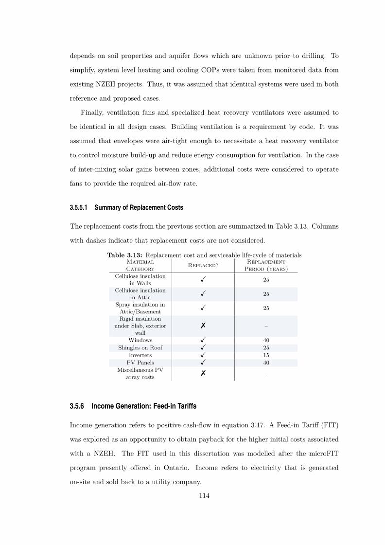
depends on soil properties and aquifer flows which are unknown prior to drilling. To

simplify, system level heating and cooling COPs were taken from monitored data from

existing NZEH projects. Thus, it was assumed that identical systems were used in both

reference and proposed cases.

Finally, ventilation fans and specialized heat recovery ventilators were assumed to

be identical in all design cases. Building ventilation is a requirement by code. It was

assumed that envelopes were air-tight enough to necessitate a heat recovery ventilator

to control moisture build-up and reduce energy consumption for ventilation. In the case

of inter-mixing solar gains between zones, additional costs were considered to operate

fans to provide the required air-flow rate.

3.5.5.1 Summary of Replacement Costs

The replacement costs from the previous section are summarized in Table 3.13. Columns

with dashes indicate that replacement costs are not considered.

Table 3.13: Replacement cost and serviceable life-cycle of materialsMaterialCategory Replaced? Replacement

Period (years)Cellulose insulation

in Walls � 25

Cellulose insulationin Attic � 25

Spray insulation inAttic/Basement � 25

Rigid insulationunder Slab, exterior

wall� –

Windows � 40Shingles on Roof � 25

Inverters � 15PV Panels � 40

Miscellaneous PVarray costs � –

3.5.6 Income Generation: Feed-in Tariffs

Income generation refers to positive cash-flow in equation 3.17. A Feed-in Tariff (FIT)

was explored as an opportunity to obtain payback for the higher initial costs associated

with a NZEH. The FIT used in this dissertation was modelled after the microFIT

program presently offered in Ontario. Income refers to electricity that is generated

on-site and sold back to a utility company.

114

The Ontario micro Feed-in Tariff (microFIT) program presently offers the most com-

petitive feed-in tariff for photovoltaic (PV) generated electricity in North America. No

other Canadian province presently offers tariffs for renewable energy generation. Histor-

ically, as much as 80.2 ¢/kWh was offered for ground and roof-installed PV. Presently,

54.9 ¢/kWh is offered for roof-top installations up to 10kW, with a 20 year standard

contract. This PV array size can be integrated on the roof of a NZEH (Candanedo,

2011; Chen, 2009). A PV array represents a significant capital cost and incentives such

as a FIT could make a NZEH an attractive investment opportunity. The offered tariff

is not inflated over time. Thus, this incentive becomes less attractive towards the end

of the investment period.

The following assumptions were made: (i) FIT program lasted for 20 years; (ii) tariffs

are not adjusted for inflation; and (iii) future revenue is not paid if life-cycle period is

shorter than feed-in tariff period.

3.5.7 Utility Rates and Operation Costs

This section details the calculation of energy operational cost from simulated energy

consumption. Of importance isthe utility billing structure, escalation of energy prices,

and new billing methods involving smart metering.

3.5.7.1 Utility Billing Structure

Operational electricity costs can been calculated using two methods: (i) equivalent an-

nual billing rate, or (ii) breakdown of electricity fees as specified from the utility.

ASHRAE (2011c) recommends a breakdown of energy costs using daily charges, peak

load charges and charges based on total use to estimate annual electricity costs from

an energy model. This method would be appropriate if the objective was to calculate

operating costs at hourly or shorter periods. However, since the objective was to evaluate

energy operations costs over an annual period, an equivalent annual billing rate was used.

3.5.7.2 Energy Escalation Rates

The cost of energy is rising in Canada. This is partially due to limited fossil fuel reserves,

conflicts in oil producing countries, as well as investments made by utilities to incorporate

115

renewable energy into their energy stocks. The increased cost due to escalating energy

prices can be calculated using equation 3.22 (Doty and Turner, 2012):

Cn = Co · (1 + e)n (3.22)

where: Cn is the annual electricity billing rate at year n ($/kWh); Co is the annual

electricity billing rate at year 0; e is the energy escalation rate.

Energy cost escalation rate = 1.97%, which is calculated as the average of energy

escalation rate between 2004 and 2008 for residential use in Montréal (Hydro-Québec,

2010)

3.5.7.3 Time of Use Rates

Many utility providers have mandated that smart meters be installed in all residential

and commercial buildings. Smart meters have been installed in almost every home and

business served by utility providers in Ontario and BC. Time of Use Billing (TOU)

enables utilities to influence peak grid demands by charging clients more during peak

periods. It is likely that TOU will be common place in most Canadian locations.

TOU rates imply that the price of electricity will depend on the time of day it is

used, as recorded by a local smart meter. The cost of electricity will increase during

peak hours, see Table 3.14. Peak hours are defined by the utility, but typically are the

hours in which electricity demand is the highest.

Table 3.14: Time of use billing

Pricing Schedule Hours TOU Price (¢)Summer Weekdays 21:00–07:00 off-peak 5.3

07:00–11:00 mid-peak 8.011:00–17:00 on-peak 9.917:00–21:00 mid-peak 8.0

Winter Weekdays 21:00–07:00 off-peak 5.307:00–11:00 on-peak 9.911:00–17:00 mid-peak 8.017:00–21:00 on-peak 9.9

Weekends and Holidays 00:00–24:00 off-peak 5.3

TOU was calculated by post-processing hourly EnergyPlus results and implementing

billing schedules based on Table 3.14. Note that since TOU results require detailed

simulation data, updating billing rates could not be calculated from the database and

116

required additional energy simulations.

3.5.8 Location Cost Multipliers

The incorporation of detailed location specific material and labour costs is unrealistic for

a research optimization study. Location factors are used from the most recent RSMeans

cost database (RSMeans, 2013). RSMeans recommends that linear multipliers be used

to convert costs from one location to another, see Table 3.15. RSMeans uses American

currency. In 2012, Canadian and American currency were at parity so this data could

be used directly.

Table 3.15: RSMeans location multipliers (RSMeans, 2013)

City Province Residential Cost MultiplierMontréal Québec 1.18Regina Saskatchewan 1.07Toronto Ontario 1.18

Vancouver British Columbia 1.10

3.5.9 Other Economic Metrics

Although NPV is the preferred method to establish cost performance, it alone is insuffi-

cient to properly characterize important elements of a building’s cost. A few additional

cost metrics are used in this thesis: (i) internal rate of return; (ii) mortgage loans;

(iii) simple payback; and (iv) capital payback. This metrics are discussed the following

sections.

3.5.9.1 Internal Rate of Return

Internal rate of return or return on investment (ROI), see equation 3.23, is the rate

of return, or discount rate, at which an investment yields a NPV of zero, or in other

words, the investment becomes cost-neutral. An advantage of this cost metric is that

options can quickly be compared over their life-cycle. However, IRR not able to clearly

represent non-simple cash flows, such as positive and negative cash flow. Problems arise

when costing of mutually exclusive projects, which is common in an energy efficiency

measure (Doty and Turner, 2012):

117

NPV =N∑

t=0

Rt

(1 + r)t= 0 (3.23)

where:

Rt Net-cash flow at time, t. Net meaning Rt = cashout − cashin

r: internal rate of return, average percent growth at which an invest becomes cost

neutral

N : number of years considered in the life-cycle (t=0 is the present year).

3.5.9.2 Mortgage Loan

A mortgage loan is a loan secured by the ownership of property. Mortgages allow for a

large initial loan amount to be paid over an agreed time period for an interest penalty.

Mortgages can be issued at a fixed interest rate or at an adjustable rate. Fixed-rate

mortgages typically have higher borrowing rates due to the perceived risk that the rate

might be less than inflation over the period of the loan. Adjustable mortgage rates are

recalculated annually based on market indexes. The following discusses details related

to a fixed-rate mortgage. Note, other fees such as application, origination and title fees

are not included.

Equation 3.24 shows the monthly payment, c, due to maintain a mortgage loan of

principle, Po (CMHC, 2012).

c = Po · rAP R

1 − (1 + rAP R)−M(3.24)

where: (a) Po is the principle loan amount (b) M is the number of monthly payments,

ex. 30 year mortgage will have 30 · 12 = 360 payment cycles (c) rAP R is the annual

percent rate (APR), split by the number of payment cycles each year, ex. monthly

payments with a 6.5% APR, rAP R = 6.5/100/12 = 0.0054

Most banks require that a down-payment be made to secure a mortgage. The best

interest rates for a Canada Mortgage and Housing Corporation (CMHC) insured loan,

require a down payment of 20% or more for a 25 year mortgage (CMHC, 2012). For

the purpose of this thesis, mortgage loans are assumed to have a 25 year repayment118

period with a 20% initial payment on the principle. Note in Canada, mortgages are

compounded every 6 months; this effects how annual interest rates are calculated.

The balance owing at after any month, m, is given by equation 3.25 (CMHC, 2012):

Pn = Po · (1 + r)m − c · (1 + r)m − 1r

(3.25)

where: (a) Po is the principle loan amount; (b) m is the number of monthly payments

made; (c) r is the annual percent rate (APR); (d) c is the monthly mortgage payment,

see equation 3.24

An assumption was made that additional technology and energy conservation and

efficiency measures were covered by a mortgage with the initial home purchase. This

reduced the initial cost of technology but increased the life-cycle cost.

3.5.9.3 Simple Payback

Simple payback is the initial capital cost divided by the annual operational savings, see

equation 3.26 (Doty and Turner, 2012). It can be used roughly estimate the time, in

number of years, required to recover an initial investment.

tsp = R0

Cann(3.26)

This metric can be used for relatively quick paybacks, say less than three years, but

is inappropriate to be used as a primary cost metric for investments beyond a three year

horizon; simple paybacks do not consider the time value of money. Life-cycle cost is

a more appropriate decision making metric as it considers inflation and cost escalation

rates.

3.5.9.4 Capital Payback

Capital payback is the period of time required for an investment to payback the initial

capital invested while considering the time value of money (Doty and Turner, 2012).

This is a key cost metric of a life-cycle cash-flow. The capital payback is calculated

by identifying the year where the cumulative cash-flow diagram passes from a negative

cash-flow to a positive cash-flow.

Figure 3.35 shows an example cash-flow diagram for an life-cycle comparison of a

119

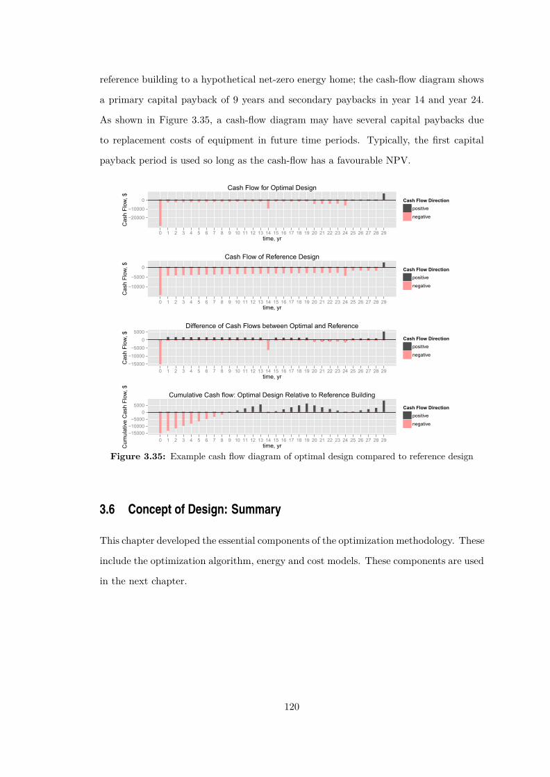
reference building to a hypothetical net-zero energy home; the cash-flow diagram shows

a primary capital payback of 9 years and secondary paybacks in year 14 and year 24.

As shown in Figure 3.35, a cash-flow diagram may have several capital paybacks due

to replacement costs of equipment in future time periods. Typically, the first capital

payback period is used so long as the cash-flow has a favourable NPV.

−20000

−10000

0

0 1 2 3 4 5 6 7 8 9 10 11 12 13 14 15 16 17 18 19 20 21 22 23 24 25 26 27 28 29

Cash Flow for Optimal Design

time, yr

Cas

h Fl

ow, $ Cash Flow Direction

positive

negative

−10000

−5000

0

0 1 2 3 4 5 6 7 8 9 10 11 12 13 14 15 16 17 18 19 20 21 22 23 24 25 26 27 28 29

Cash Flow of Reference Design

time, yr

Cas

h Fl


positive

negative

−15000

−10000

−5000

0

5000

0 1 2 3 4 5 6 7 8 9 10 11 12 13 14 15 16 17 18 19 20 21 22 23 24 25 26 27 28 29

Difference of Cash Flows between Optimal and Reference

time, yr

Cas

h Fl


positive

negative

−15000−10000−5000

05000

0 1 2 3 4 5 6 7 8 9 10 11 12 13 14 15 16 17 18 19 20 21 22 23 24 25 26 27 28 29

Cumulative Cash flow: Optimal Design Relative to Reference Building

time, yrCum

ulat

ive

Cas

h Fl

ow, $

Cash Flow Directionpositive

negative

Figure 3.35: Example cash flow diagram of optimal design compared to reference design

3.6 Concept of Design: Summary

This chapter developed the essential components of the optimization methodology. These

include the optimization algorithm, energy and cost models. These components are used

in the next chapter.

120

Chapter 4

Multi-Objective Optimal Design of a Near

Net-Zero Energy Solar House

“Few things are harder to put up with than the annoyance of a good example.–Mark Twain ”

4.1 Overview

This chapter presents a redesign case study of the ÉcoTerraTM house1. This

research originated as a conference paper (Bucking et al., 2010). A modified

version was accepted for publication in ASHRAE Transactions (Bucking et al., 2013a).

This chapter uses the optimization methodology presented in chapter 3 including the

optimization algorithm (section 3.2), energy model (section 3.4) and cost model (sec-

tion 3.5). This chapter builds the concept of the archetype solar home that combines

passive solar design, energy efficiency measures including a geothermal heat pump and

a building-integrated photovoltaic system. This archetype is used in later chapters as a

case-study.

This chapter shows how strategic deterministic searches can be deployed using infor-

mation extracted from a database to improve performance of an evolutionary algorithm.

The information extraction approach was previously described in section 3.3.8. These

findings in improving algorithm performance are incorporated into an information driven

EA presented in Chapter 5.1ÉcoTerra is a registered trade-mark of Alouette homes.

121

4.2 Background

ÉcoTerraTM is a detached near NZE home located in Eastman, Québec, see Figure 4.1.

This home was one of the winners of the Canadian Mortgage and Housing Corporation

Equilibrium Net Zero Energy Home competition and the first demonstration house built

under this program (CMHC, 2008). The primary goal of the house design was to be

cost competitive with other pre-fabricated homes, while greatly reducing energy intensity

compared to the Canadian building stock.

Figure 4.1: ÉcoTerra House.

The ÉcoTerra design has a heated floor area of 211.1 m2 (2,272 ft2) and a heated

volume of 609.1 m3 (21,510 ft3). The house is heated and cooled using a well-tied

ground source heat pump (GSHP). Domestic hot-water (DHW) energy consumption

is offset using a desuperheater and thermal energy collected from an open-loop solar

thermal collector on the roof surface. The design features an innovative dual-energy

roof system which uses 6% efficient amorphous silicon photovoltaic (PV) panels and an

air-channel to simultaneously collect thermal and electrical energy.

The ÉcoTerra home was the first pre-fabricated home design with a customized

building-integrated photovoltaic/thermal (BIPV/T) roof linked to a hybrid thermal en-

ergy storage system (Chen et al., 2010a,b). This technology combined with passive solar

design strategies resulted in an annual net-energy consumption less than 50kWh/m2, or

one fifth of the average national energy consumption or one half of the R2000 standard,

see Figure 4.2 (Doiron et al., 2011). R2000 is a voluntary standard which promotes

cost-effective energy-efficient building practices and technologies in Canada.122

Figure 4.2: ÉcoTerra annual energy consumption (Doiron et al., 2011).

Figure 4.3: ÉcoTerra System schematic (Chen, 2009).

123

Approximately 40% percent of the gross heating demand is met through passive solar

gains. Some thermal energy is offset by the roof integrated 2.84 kWe BIPV/T system,

which can produce up to 10 kWp of useful heat (Candanedo et al., 2010). The remaining

auxiliary heating is provided by a GSHP. The thermal energy from the BIPV/T is

delivered directly through an open-loop air system to a concrete slab in the basement

or to a DHW pre-heat tank through an air-water heat exchanger, see Figure 4.3 (Chen,

2009). The slab serves as an active charge/passive discharge storage device.

Data was recorded from early 2008 until 2012 using over 100 temperature sensors

distributed within the roof, slab and thermal zones. The PV generation, DHW and

heat pump electrical demand of the home was monitored separately. This information

permits the study of each design parameter and offers a unique opportunity to evaluate

the present operation as well as to assess the impact of design improvements.

4.3 Method and Problem Formulation

Two redesign approaches were used in this chapter: (1) identify minor upgrades that

could help ÉcoTerra reach NZE or reduce life-cycle costs without significant design

modification, and (2) perform a full redesign with significant design modifications and

a feed-in tariff to reduce operational costs.

For the first redesign approach, upgrades were restricted to simple renovations and

control strategies modifications. These included modifying envelope insulation, air-

sealing, and fine-tuning control strategies. Geometry, orientation, roof area and slope

were fixed. Adding more PV panels was allowed if a similar PV product was used to

match the æsthetic and electrical characteristics of the existing PV strings.

In the second redesign approach, the complete design was reconsidered including

all aspects of passive solar design, renewable energy generation and control strategies.

Changes to the rectangular shape were allowed only if the same floor area and number

of floors were used. A feed-in tariff created revenue from on-site PV generated electric-

ity. Including an incentive shows how economics can influence optimal building design

approaches.

Additional goals of this study are to: (i) evaluate the potential of hybrid deterministic-

124

evolutionary algorithms in design optimization, (ii) extract information regarding vari-

able interdependencies, and (iii) expedite the optimization process using extracted in-

formation.

The information extraction approach was previously described in section 3.3.8.

The design of net-zero energy solar buildings is dependent on local climate and site

constraints. Any significant deviations in heating or cooling degree days or the amount

of solar exposure would require the optimization process to be repeated on a new design.

This fact precludes the utility of training methods such as decision tree ensembles and

neural networks. However, restarting the entire optimization process is unnecessary as

previous simulation data can be used to identify the relative importance of each design

variable and suggest possible search strategies. There will be similarities between many

optimal design parameters in elite design, even across different locations.

To complete the study, an energy model, database and optimization algorithm were

necessary. This components were previously discussed in chapter 3. SQLite was used as

a database to store variable mappings and fitness evaluations (SQLite, 2012).

The objective of the case-study was to conduct a multi-objective optimization analy-

sis using net annual electricity consumption and the life-cycle cost. Time-of-use electric-

ity billing and feed-in tariffs will change design variable interactions and are considered

in chapter 7.

Design variables included in the optimization have been restricted to upgrades that

could be done via simple renovation and control strategies to reduce electricity consumed

for heating and cooling loads such as blind controls; free cooling and modifications to

temperature schedules. Adding more PV was allowed if the type and efficiency remained

the same (6% efficient amorphous silicon), but changes to the roof slope were prohibited.

An exhaustive list of design variables used for the optimization and parameters for the

ÉcoTerra design are presented in Table 4.1. Note that glazing types and WWR were

considered separate design variables for all four walls.

The following sections elaborate on the energy model, optimization algorithm, strate-

gies to integrate deterministic searches into an evolutionary algorithm and methods to

extract information regarding design variable importance and interdependencies.

125

Table 4.1: Definition of optimization variables and parameters used for the Ecoterra redesignstudy

Variable Units Min. Max. No. Steps EcoTerra Description

wall_ins m2K/W 3.50 12 8 5.89 Effective resistance of wall insula-tion

ceil_ins m2K/W 5.6 15 8 8.2 Effective resistance of ceiling insu-lation

base_ins m2K/W 0 7 8 5.2 Effective resistance of basementwall insulation

slab_ins m2K/W 0 2.32 4 1.32 Effective resistance of slab insula-tion

ovr_south m 0 0.45 4 0 Width of southern window over-hangs

int_loads % CADavg 50 80 8 50 Occupant loads (% Canadian aver-age consumption)

pv_area % 0 90 8 50 Percent of PV area on roofwwr_s % 1 80 8 35 Window to Wall Ratio South (also

N,E,W)GT_s – 1 4 1 4 Glazing type (also N,E,W)set_heat ◦C 18 25 4 22 Heating setpointset_cool ◦C 25 28 4 26 Cooling setpointFT – 1 2 2 2 Window framing types (ex.

1:Wood, 2:Vinyl)blind_irr W/m2 0 1000 4 500 Incident solar radiation for blind

deploymentslab_th m 0.1 0.2 8 0.1 Concrete slab thicknessvwall_th m 0 0.35 8 0.1 Concrete wall thicknesszone_mix L/s 0 400 4 400 Air circulation rate between ther-

mal zonesinfil ACH 0.025 0.179 8 0.047 Natural infiltration rate

4.4 Energy and Cost Model

Details regarding the energy model were described previously in section 3.4.

The cost model was described previously in section 3.5.

4.5 Optimization Algorithm

A summary of algorithm parameters and setting used for this study is summarized in

Table 4.2. A 54 grey-coded binary string was used to represent each candidate build-

ing design. Two types of recombination were used. The first shares data between two

parents on a bit-by-bit basis using a uniform crossover and the second shares data on a

variable-by-variable basis. Uniform recombination on a variable-by-variable basis should

be included as it is unlikely that a binary string representing a sensitive design parameter

will be transferred from a parent to a candidate child for a representation greater than 50

bits, an important aspect in convergence to optimal solutions. Diversity was measured

by averaging the number of bits that any individual shared with the elite member in the126

population (lowest annual net-electricity consumption). Diversity control becomes im-

portant for small population sizes, where there is a risk that the population prematurely

converges to a local minimum, or the average diversity in the population converges to

one. The problem was fixed by injecting noise into the population by increasing mutation

rates and decreasing tournament sizes in the event of collapsing diversity. The concept of

injecting noise to escape local minima is found in many optimization algorithms catered

to navigating highly multi-modal solution spaces (Eiben and Smith, 2003). A more elab-

orate discussion of algorithm configuration and performance is presented in the concept

of design, see section 3.2.

Table 4.2: Summary of algorithm configuration

Algorithm Parameter Setting

Representation 54 bit binary stringPopulation Size 10Recombination 50% bit-by-bit Uniform, 50% variable UniformRecombination Prob 100%Mutation bit-by-bit mutationMutation Prob 1.5%Elitism? Yes, best individualParent Selection NSGA-II, see section 3.3.7No. of Children 10Survivor Selection Best of parents and children, (μ+λ)Diversity Control NSGA-II crowding distances

It is well known that Evolutionary Algorithms work well at finding good combina-

tions of design parameters, but are less adapted to resolve local minima without a ‘lucky’

random effect (Eiben and Smith, 2003). Resolving local minima, or search intensifica-

tion, is the expertise of a deterministic search. Deterministic searches were attempted:

(i) after initial population fitness evaluation, (ii) as a mutation operator, and (iii) after

the termination criteria was reached.

A hill climbing algorithm was used for the deterministic search. The hill climbing

search increments or decrements each design parameter such that the fitness function

is reduced. The process was repeated across each design variable and variable setting

until the fitness function could not be further reduced.

The most effective way to extract variable interdependencies at a defined energy

consumption interval was to use the Mutual Information (MI) shared between two design

127

variables. This was described previously in section 3.3.8.4. Variables having low MI were

targeted for hill-climbing searches.

Results and a discussion are presented in the following section.

4.6 Results and Discussion

Recall that two redesign approaches were used in this chapter: (1) identify minor up-

grades that could help ÉcoTerra reach NZE for minimal life-cycle cost without sig-

nificant design modification, and (2) perform a full redesign with significant design

modifications and a feed-in tariff to reduce operational costs. The first multi-objective

redesign study is show in Figure 4.4.

4000 6000 8000 10000 12000 14000 16000Net-Energy Consumption, kWh

60000

80000

100000

120000

140000

160000

180000

Net-PresentValue,CAD$

Raw Optimization Data

Pareto Front

Ecoterra

Figure 4.4: Multi-objective constrained redesign of ÉcoTerra home.

From Figure 4.4, the best design found had a net energy consumption of 5300kWh,

a decrease in energy intensity from 50 kWh/m2 to 20 kWh/m2. Important changes

included adding PV to the remaining area of the roof and modifying the heating and

cooling dead-band limits, resulting in a combined net-electricity consumption reduction

of 3500kWh. Of the redesign opportunities identified, none required significant changes

to the passive solar design of the house. For example, fine tuning the thermal storage

(slab and basement wall), increasing the slab and wall insulation levels, increasing the

128

southern window area to 50%, increasing air tightness to 0.5 ACH at 50Pa (approxi-

mately 0.025 ACH natural infiltration rate) from 0.8 ACH at 50Pa (approximately 0.047

ACH natural infiltration rate), cumulatively amounted to only 500kWh of annual elec-

tricity savings. This indicates that the ÉcoTerra design was near a local optimum

with regards to passive solar design.

Figure 4.5 shows results for the second part of the redesign case-study. In this part,

all variables were reconsidered including PV panel efficiency, roof-slope, orientation and

geometry. Note that all designs were compliant with local building codes. The diversity

in results shows that there significant opportunity to better improve energy codes and

reduce energy consumption and life-cycle cost of residential homes in Canada.

-10000 -5000 NZE 5000 10000 15000Net-Energy Consumption, kWh

50000

100000

150000

200000

250000

300000

350000

Net-PresentValue,CAD$


Pareto Front

Ecoterra

Figure 4.5: Multi-objective complete redesign of ÉcoTerra home.

The primary inhibitor to NZE with the ÉcoTerra design is the lack of renewable

energy generation. More than doubling the PV efficiency from 6% to 15% alone would

reduce net-electricity consumption from 5300kWh to 400kWh. A secondary inhibitor was

high appliance loads which were measured from monitored data to be approximately

4000kWh/yr. Further research on implementing conservation measures on appliance,

lighting, and DHW loads and their effect on occupant energy behaviour is recommended.

Although Figure 4.5 shows a spectrum of costs and energy consumption, we shall

consider a single optimal design to examine improvements. The optimal design with129

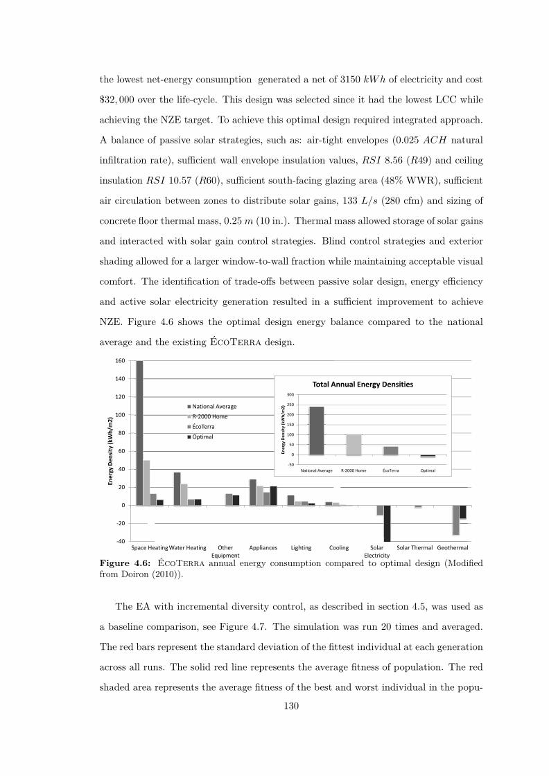
the lowest net-energy consumption generated a net of 3150 kWh of electricity and cost

$32, 000 over the life-cycle. This design was selected since it had the lowest LCC while

achieving the NZE target. To achieve this optimal design required integrated approach.

A balance of passive solar strategies, such as: air-tight envelopes (0.025 ACH natural

infiltration rate), sufficient wall envelope insulation values, RSI 8.56 (R49) and ceiling

insulation RSI 10.57 (R60), sufficient south-facing glazing area (48% WWR), sufficient

air circulation between zones to distribute solar gains, 133 L/s (280 cfm) and sizing of

concrete floor thermal mass, 0.25 m (10 in.). Thermal mass allowed storage of solar gains

and interacted with solar gain control strategies. Blind control strategies and exterior

shading allowed for a larger window-to-wall fraction while maintaining acceptable visual

comfort. The identification of trade-offs between passive solar design, energy efficiency

and active solar electricity generation resulted in a sufficient improvement to achieve

NZE. Figure 4.6 shows the optimal design energy balance compared to the national

average and the existing ÉcoTerra design.

-40

-20

0

20

40

60

80

100

120

140

160

Space Heating Water Heating Other Equipment

Appliances Lighting Cooling Solar Electricity

Solar Thermal Geothermal

Ener

gy D

ensi

ty (k

Wh/

m2)

National Average

R-2000 Home

ÉcoTerra

Optimal

-50

0

50

100

150

200

250

300

National Average R-2000 Home ÉcoTerra Optimal

Ener

gy D

ensi

ty (k

Wh/

m2)

Total Annual Energy Densities

Figure 4.6: ÉcoTerra annual energy consumption compared to optimal design (Modifiedfrom Doiron (2010)).

The EA with incremental diversity control, as described in section 4.5, was used as

a baseline comparison, see Figure 4.7. The simulation was run 20 times and averaged.

The red bars represent the standard deviation of the fittest individual at each generation

across all runs. The solid red line represents the average fitness of population. The red

shaded area represents the average fitness of the best and worst individual in the popu-

130

lation across the 20 simulation runs. The solid black line is the average diversity of the

population, a measure of the average number of bits shared with the elite individual in

that particular generation. It can be concluded that, on average, 160 energy simulations

are required to find an optimal building design with a fitness of 5536 kWh.

Figure 4.7: Average of 20 runs of the baseline EA

Of the three identified locations for deterministic search integration only one was

found to be of significance. Searching sensitive design variables after the initialization of

the population was the best way to integrate deterministic searches into a single hybrid

deterministic-evolutionary approach. For instance, the fittest individuals always maxi-

mized the available roof area to offset unavoidable user loads. The relative importance

of each design variable was decided on by randomly selecting a building design and cal-

culating, variable-by-variable, the steepest descent to the best known building design.

Variables that interacted weakly with the population were considered to be indepen-

dent and could be locked after a brief search. Each design variable that was lockable

contracted the size of the solution space significantly and expedited the search process.

By using a hybrid deterministic-evolutionary algorithm, identification of optimal designs

could be reproduced by deterministically searching the PV area and occupant load vari-

ables and as few as five evolutionary generations to result in a building design with a

fitness of 5306 kWh, see Figure 4.8.

Initiating a deterministic search at the end of the evolutionary algorithm successfully

131

Figure 4.8: Average of 20 runs of hybrid EA

resolves designs to local minima, but required a substantial amount of computations,

often as much as the original EA, for a negligible improvement in fitness. This was

primarily because the model had already maximized renewable energy generation and

was trying to further reduce heating and cooling loads, but any improvements were

devalued by the Coefficient of Performance (COP) of the heat pump, that is, reduced by

a factor of one third. This result enforces the idea that there is little benefit in finding

the truly optimal design since the surrounding design space is nearly as good for this

specific case study.

Probabilistically incrementing or decrementing the setting of a design parameter as a

mutation operator was inadequate to inject diversity into the population. As previously

mentioned, the purpose of the mutation operator is to explore new territory in the

solution space and if necessary, to intentionally randomize the population to escape

from local minima. Randomly incrementing or decrementing the setting of a design

parameter was simply not random enough to escape from local minima.

In conclusion, the importance of an evolutionary algorithm is to find good design

variable combinations quickly and locate near optimal solutions. Deterministic searches

are best used to initiate a steepest descent search on sensitive variables prior to the

evolutionary search.

132

Variable interactions for all buildings with energy consumption of less than 6500kWh

are shown in Figure 4.9. Variable interactions were extracted using techniques discussed

in the section 3.3.8.4. Design variables that form their own hierarchy could be highly

sensitive to setting variations or could be very weakly interacting with all other design

variables. Either situation indicates that the variable is susceptible to a deterministic

search. For example, the PV area and occupant behaviour interact weakly with other

design variables, but exhibit some mutual interactions as PV is used to offset electri-

cal loads. Sub-clusters identify variables that are better handled by the evolutionary

algorithm due to design variable interdependencies.

Figure 4.9: Dendrogram of variable interactions where inverse mutual information is used as adistance metric, using agglomerative clustering (complete method with Canberra distance)

Figure 4.10 shows the back-tracking search, core concept in section 3.3.8.1, from

the initial ÉcoTerra design, to the optimal solution found in the defined solution

space. Note that the first ten parameters have the largest impact on fitness, as they

open new solution space landscapes and that the last few parameter changes are largely

inconsequential. This is due to the fact that they were either near optimal values, or are

insensitive to variations in the vicinity of the solution space landscape (they may be very

sensitive at a different region of search space). Important changes included adding PV to

the remaining area of the roof and modifying the heating and cooling dead-band to the

limits of ASHRAE thermal comfort, resulting in a combined net-electricity consumption

133

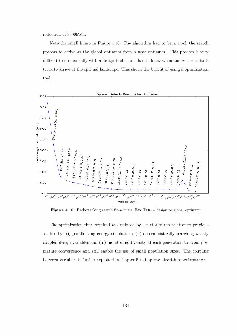
reduction of 3500kWh.

Note the small hump in Figure 4.10. The algorithm had to back track the search

process to arrive at the global optimum from a near optimum. This process is very

difficult to do manually with a design tool as one has to know when and where to back

track to arrive at the optimal landscape. This shows the benefit of using a optimization

tool.

Figure 4.10: Back-tracking search from initial ÉcoTerra design to global optimum

The optimization time required was reduced by a factor of ten relative to previous

studies by: (i) parallelizing energy simulations, (ii) deterministically searching weakly

coupled design variables and (iii) monitoring diversity at each generation to avoid pre-

mature convergence and still enable the use of small population sizes. The coupling

between variables is further exploited in chapter 5 to improve algorithm performance.

134

Chapter 5

An Information Driven Hybrid Evolutionary

Algorithm for Optimal Building Design

“In God we trust, all others bring evidence.–W. Edwards Deming ”

5.1 Overview

This chapter proposes a hybrid evolutionary algorithm which utilizes information

gained during previous simulations to expedite and improve algorithm conver-

gence using targeted deterministic searches. This chapter builds on the success of strate-

gic deterministic searches first explored in chapter 4. Strategic deterministic searches

are now integrated into the EA. Similar to the earlier chapters, this chapter uses the

archetype solar home that combines passive solar design, energy efficiency measures

including a geothermal heat pump and a building-integrated photovoltaic system previ-

ously described in chapter 4. This methodology was published and peer reviewed in a

Solar Energy paper (Bucking et al., 2013b).

5.2 Background

Most previous research involving building simulation and optimization algorithms em-

phasized the importance of identifying a single optimal solution or a set of Pareto optimal

solutions, see chapter 2. However, optimization algorithms extract other valuable in-

135

formation about the design problem during the optimization process, which is seldom

used. Of equal importance is the collection and use of information gained during the

optimization process. For example, other interesting information is the identification

of: (i) automated search and discovery of potential optimal designs which best achieve

desired performance objectives; and (ii) consideration of conflicting system level design

trade-offs. Data-mining within the optimization process allows for a broader knowledge

of the design problem and the feasible solution set. The inclusion and application of

information obtained during the search process still remains unexplored in BPS.

This chapter proposes a method to extract and strategically apply information gained

within an optimization algorithm to improve search resolution and expedite algorithm

convergence for building simulation problems.

Since each building simulation problem has a unique set of constraints, climate con-

ditions, shape characteristics and occupant usage characteristics, optimization studies

must inevitably be performed on a case-by-case basis. Reducing time requirements for

optimization studies while improving search resolution is an important research area of

BPS.

The utilization of information obtained during the search process still remains unex-

plored in building optimization research. This paper proposes a data-mining technique

within the optimization process. A new algorithm is presented to extract and strate-

gically apply information gained using sub-searches to improve search resolution and

expedite algorithm convergence for building simulation problems.

This chapter contains the following sections. Section 5.3 presents the proposed

methodology, and the algorithm is applied to a case study in section 5.4. Discussions of

results are presented in section 5.5, followed by conclusions.

5.3 Methodology

This section integrates strategic deterministic search, first explored in chapter 4, into

the EA. Two evolutionary algorithms are proposed.

In addition, effective search strategies are borrowed from other optimization algo-

rithms and incorporated into the proposed EA. For example, pseudo-differential gradi-

136

ents originating from DE were explored as a mutation operator. Hill-climbing searches

from the deterministic family are examined to perform searches on isolated design vari-

ables. The proposed optimization algorithms are discussed in the next section.

5.3.1 Proposed Optimization Algorithms

Two algorithms are used in this chapter, a modified evolutionary algorithm (previously

presented in section 3.3) and an information-driven hybrid evolutionary algorithm (sec-

tion 5.3.1.2). The performance of both algorithms are benchmarked and discussed in

later sections.

5.3.1.1 Proposed Modified Evolutionary Algorithm (EA)

Recall that three innovations, presented previously in section 3.3, were applied typical

EA to improve algorithm performance: (i) mixed crossover operations (inside and out-

side representations), (ii) mixed mutation operators (differential mutation and bit-flip

mutation), and (iii) algorithm parameter control using diversity measurements.

5.3.1.2 Incorporation of Mutual Information into a Hybrid Evolutionary Algorithm (MIHEA)

The proposed EA from the previous section was augmented with a module to data-mine

previous simulation information. This hybrid EA was developed to extract information

regarding variable interdependencies and strategically deploy deterministic searches to

improve algorithm performance.

EAs are best suited for finding near-optimal solutions and there is no guarantee that

searches will resolve to absolute minima. Deterministic searches are better suited for

resolving local minima, or search intensification. In building optimization, interactions

between variables are treated as a hindrance when they could improve the search process.

For example, weakly dependent design variables might be susceptible to deterministic

searches. Similarly, if interactions are identified between sub-clusters of design variables,

sub-population search strategies might expedite the search process.

A hill-climbing algorithm was used for the deterministic search. A hill-climbing

search increments or decrements each design parameter such that fitness is improved.

The difficulty lies in identifying which design variables may be weakly interacting and

137

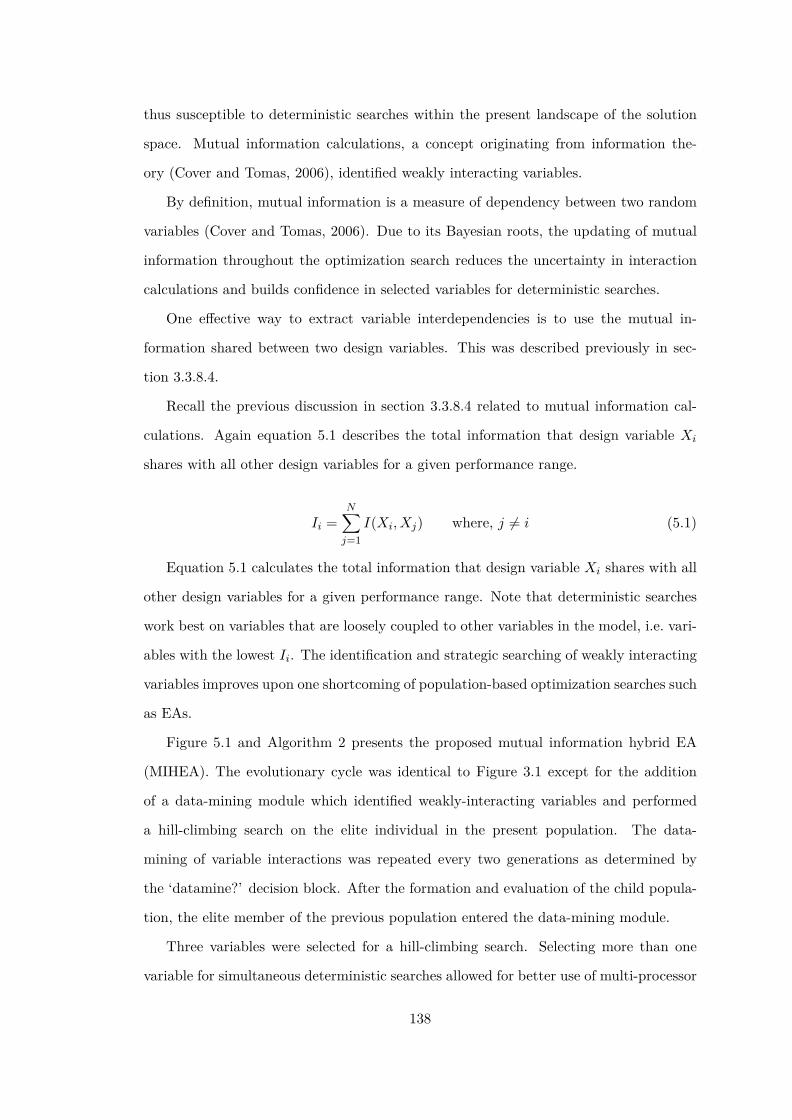
thus susceptible to deterministic searches within the present landscape of the solution

space. Mutual information calculations, a concept originating from information the-

ory (Cover and Tomas, 2006), identified weakly interacting variables.

By definition, mutual information is a measure of dependency between two random

variables (Cover and Tomas, 2006). Due to its Bayesian roots, the updating of mutual

information throughout the optimization search reduces the uncertainty in interaction

calculations and builds confidence in selected variables for deterministic searches.

One effective way to extract variable interdependencies is to use the mutual in-

formation shared between two design variables. This was described previously in sec-

tion 3.3.8.4.

Recall the previous discussion in section 3.3.8.4 related to mutual information cal-

culations. Again equation 5.1 describes the total information that design variable Xi

shares with all other design variables for a given performance range.

Ii =N∑

j=1I(Xi, Xj) where, j = i (5.1)

Equation 5.1 calculates the total information that design variable Xi shares with all

other design variables for a given performance range. Note that deterministic searches

work best on variables that are loosely coupled to other variables in the model, i.e. vari-

ables with the lowest Ii. The identification and strategic searching of weakly interacting

variables improves upon one shortcoming of population-based optimization searches such

as EAs.

Figure 5.1 and Algorithm 2 presents the proposed mutual information hybrid EA

(MIHEA). The evolutionary cycle was identical to Figure 3.1 except for the addition

of a data-mining module which identified weakly-interacting variables and performed

a hill-climbing search on the elite individual in the present population. The data-

mining of variable interactions was repeated every two generations as determined by

the ‘datamine?’ decision block. After the formation and evaluation of the child popula-

tion, the elite member of the previous population entered the data-mining module.

Three variables were selected for a hill-climbing search. Selecting more than one

variable for simultaneous deterministic searches allowed for better use of multi-processor

138

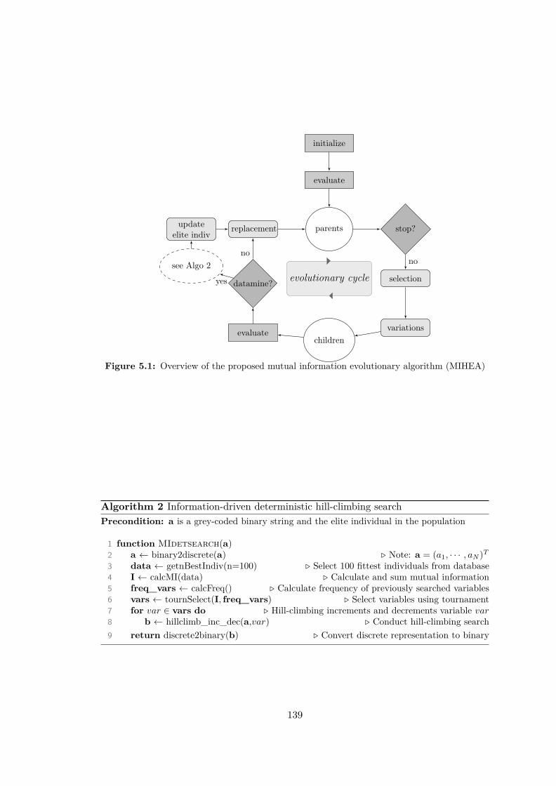
initialize

evaluate

parents stop?

selection

variations

children

replacement

datamine?

evaluate

updateelite indiv

see Algo 2

evolutionary cycle

nono

yes

Figure 5.1: Overview of the proposed mutual information evolutionary algorithm (MIHEA)

Algorithm 2 Information-driven deterministic hill-climbing searchPrecondition: a is a grey-coded binary string and the elite individual in the population

1 function MIdetsearch(a)2 a ← binary2discrete(a) � Note: a = (a1, · · · , aN )T

3 data ← getnBestIndiv(n=100) � Select 100 fittest individuals from database4 I ← calcMI(data) � Calculate and sum mutual information5 freq_vars ← calcFreq() � Calculate frequency of previously searched variables6 vars ← tournSelect(I, freq_vars) � Select variables using tournament7 for var ∈ vars do � Hill-climbing increments and decrements variable var8 b ← hillclimb_inc_dec(a,var) � Conduct hill-climbing search9 return discrete2binary(b) � Convert discrete representation to binary

139

computational resources. Variables were selected for the hill-climbing search using two

criteria: (i) the mutual information shared with other design variables, and, (ii) the

frequency that each variable had been deterministically searched in all previous gener-

ations. Mutual information calculations used at most 100 unique individuals from the

database ordered by improving fitness to calculate interactions. The MIHEA selected

variables for hill-climbing searches using a tournament selection operator to identify

variables with low total mutual information, see equation 3.4, and a low frequency of

being previously hill-climbed. Tournament operators ensured that the same variables

were not searched repeatability every generation but still gave preference to variables

that were weakly interacting.

The follow section describes how the proposed algorithms were benchmarked.

5.3.2 Optimization Algorithm Performance Comparison

Comparing the performance of the proposed optimization algorithms was challenging

because both proposed EA and MIHEA algorithms depend on stochastic processes and

simulations in this study were conducted in batches on multi-core processors.

The performance of the proposed EA and MIHEA were compared to GenOpt’s parti-

cle swarm inertial weight (PSOIW) algorithm (Wetter, 2011b). Initial populations were

randomized for each optimization run to ensure that algorithms were compared under

different initial fitness landscapes. Identical design variables and variable step-sizes were

used to constrain algorithms to the same solution spaces.

The following measures compared algorithm performance: (i) sensitivity of algorithm

configurations, (ii) repeatability studies, and (iii) convergence analysis. The sensitivity

study compares the sensitivity of each algorithm to its initial configuration. In addition,

this study determines which initial configuration resulted in the best algorithm perfor-

mance. A repeatability study explores how consistently each algorithm will find optimal

or near optimal solutions and the expected fitness value for each algorithm given a single

optimization run. The repeatability study also compares algorithms to determine re-

ductions in computational and time requirements. Because the optimization algorithm

used in the study depends on stochastic processes, a significant sample of optimization

runs is required to conduct the repeatability study. Finally, a convergence analysis com-

140

pares how quickly each algorithm converges to optimal landscapes from a random initial

population.

In the following case study, we compare the performance of the proposed EA and

MIHEA to the GenOpt PSOIW algorithm. The proposed EA and MIHEA are also

compared separately to estimate the performance improvement from augmenting the

EA with information-driven deterministic searches.

5.4 Case Study: Net-Zero Energy House

The case study involves the optimization of a net-zero energy home (NZEH) located in

Montréal, Québec. The energy model was previously described in chapter 3 section 3.4.

The case study was presented previously in chapter 4. Table 5.1 shows the variables

used in this case-study.

5.4.1 Objective function

The objective of the study was to minimize the net-annual energy consumption of a

near net-zero energy home. Heating, cooling, fan loads, PV generation and lighting

loads were simulated using EnergyPlus (Crawley et al., 2000). The objective function

used for this case study was the annual net-electricity consumption of the building, see

equation 5.2,

f(x) = Qheat/COPH + Qcool/COPC + Eelec − EP V (5.2)

where: x = (x1, x2, · · · , xN )T is a design variable vector; f(x) is the annual net-

electricity consumption of the building (kWh); COP is the average annual coefficient of

performance of the ground-source heat pump in heating and cooling mode, 3.77 and 2.77

respectively; Q is the annual heating and cooling load (kWh); Eelec is the annual elec-

tricity consumption in lighting, domestic hot-water (DHW), appliances and plug-loads

(kWh) and; EP V is the electricity generated by the roof-top photovoltaic panels (kWh).

When f(x) < 0 this implies the net-generation of electricity, or a positive-energy house.

Note that variable descriptions are shown for the south orientation only; also, the

PV slope is equal to the roof slope. Table 5.2 shows the binary encoding used in the

representation for a sample of variables. Equation 5.3 demonstrates the translation of a

141

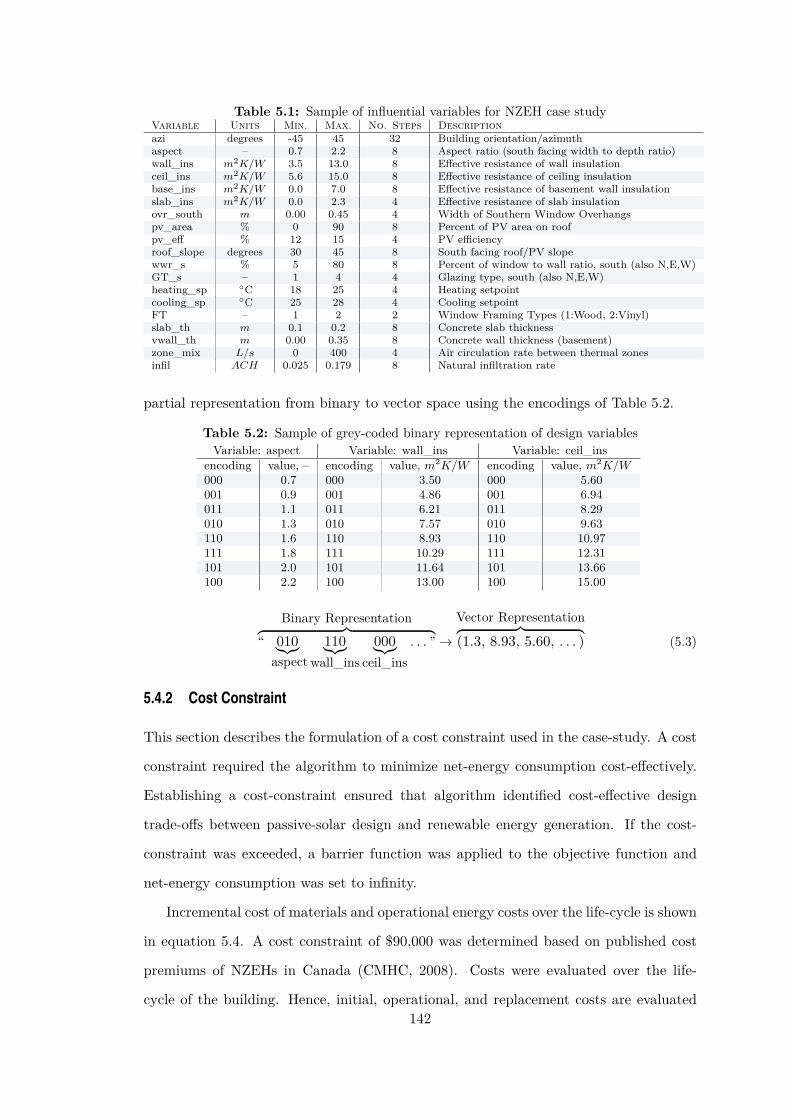
Table 5.1: Sample of influential variables for NZEH case studyVariable Units Min. Max. No. Steps Descriptionazi degrees -45 45 32 Building orientation/azimuthaspect – 0.7 2.2 8 Aspect ratio (south facing width to depth ratio)wall_ins m2K/W 3.5 13.0 8 Effective resistance of wall insulationceil_ins m2K/W 5.6 15.0 8 Effective resistance of ceiling insulationbase_ins m2K/W 0.0 7.0 8 Effective resistance of basement wall insulationslab_ins m2K/W 0.0 2.3 4 Effective resistance of slab insulationovr_south m 0.00 0.45 4 Width of Southern Window Overhangspv_area % 0 90 8 Percent of PV area on roofpv_eff % 12 15 4 PV efficiencyroof_slope degrees 30 45 8 South facing roof/PV slopewwr_s % 5 80 8 Percent of window to wall ratio, south (also N,E,W)GT_s – 1 4 4 Glazing type, south (also N,E,W)heating_sp ◦C 18 25 4 Heating setpointcooling_sp ◦C 25 28 4 Cooling setpointFT – 1 2 2 Window Framing Types (1:Wood, 2:Vinyl)slab_th m 0.1 0.2 8 Concrete slab thicknessvwall_th m 0.00 0.35 8 Concrete wall thickness (basement)zone_mix L/s 0 400 4 Air circulation rate between thermal zonesinfil ACH 0.025 0.179 8 Natural infiltration rate

partial representation from binary to vector space using the encodings of Table 5.2.

Table 5.2: Sample of grey-coded binary representation of design variablesVariable: aspect Variable: wall_ins Variable: ceil_ins

encoding value, – encoding value, m2K/W encoding value, m2K/W000 0.7 000 3.50 000 5.60001 0.9 001 4.86 001 6.94011 1.1 011 6.21 011 8.29010 1.3 010 7.57 010 9.63110 1.6 110 8.93 110 10.97111 1.8 111 10.29 111 12.31101 2.0 101 11.64 101 13.66100 2.2 100 13.00 100 15.00

Binary Representation︷︸︸︷“ 010︸︷︷︸

aspect110︸︷︷︸

wall_ins000︸︷︷︸

ceil_ins. . . ” →

Vector Representation︷︸︸︷(1.3, 8.93, 5.60, . . . ) (5.3)

5.4.2 Cost Constraint

This section describes the formulation of a cost constraint used in the case-study. A cost

constraint required the algorithm to minimize net-energy consumption cost-effectively.

Establishing a cost-constraint ensured that algorithm identified cost-effective design

trade-offs between passive-solar design and renewable energy generation. If the cost-

constraint was exceeded, a barrier function was applied to the objective function and

net-energy consumption was set to infinity.

Incremental cost of materials and operational energy costs over the life-cycle is shown

in equation 5.4. A cost constraint of $90,000 was determined based on published cost

premiums of NZEHs in Canada (CMHC, 2008). Costs were evaluated over the life-

cycle of the building. Hence, initial, operational, and replacement costs are evaluated142

using the net-present value (NPV) of each design. Cost calculations were performed by

post-processing energy simulation results.

g(x) = CNP V + ENP V + RNP V − SNP V (5.4)

≤ $90, 000

where: CNP V : is the capital costs of materials and equipment in Canadian dollars;

ENP V : is the operational energy costs calculated from energy simulation results; RNP V :

is the replacement cost for materials and equipment; and SNP V : is the salvage or

residual value using a linear depreciation method.

Materials were scheduled for replacement based on an expected serviceable life-

time (RSMeans, 2013). A marginal electricity rate of 7 cents with an escalation rate of

2.0% was used (Hydro-Québec, 2010). Note that all monetary amounts refer to Canadian

dollars. Life-cycle costs were calculated over a 30 year time horizon.

Initial costs were broken down as follows:

C = wallinsCost + ceilinsCost + baseinsCost + slabinsCost +

roofCost + overhangCost + concrCost + PVCost +

winCost + airtightCost (5.5)

where: C is the total material cost; insCost is the cost of wall, ceiling, basement and

slab insulation; winCost is the cost of windows based on glazing area; roofCost is the

incremental cost of additional roof framing beyond 30 degrees slope; overhangCost is the

cost of overhangs; concrCost is the cost of concrete walls and slab for passive thermal

storage; PVCost is the cost of PV panels and inverters; and airtightCost is the incre-

mental cost associate with tighter envelopes. These costs were specified from RS-Means

data (RSMeans, 2012, 2013).

143


To ensure that the EA and PSOIW algorithms were operating properly, the sensitivity

of several algorithm configurations were explored. The algorithm settings which resulted

in the lowest fitness values were selected for future optimization runs, see run no. 1 of

Tables 5.3 and 5.4.

Table 5.3: Parametric run for various algorithm parameters, EAEA Parameters Run 1 Run 2 Run 3 Run 4 Run 5

Representation 62 bit binarystring – – – –

Population Size 10 – – – –Recombination * 60% Method 1 60% Method 1 60% Method 2 80% Method 2 60% Method 2

Mutation � 60% Method 2 60% Method 2 60% Method 1 60% Method 1 80% Method 2Mutation Prob 2.0% 3.0% 2.0% 2.0% 1.0%Scaling Factor 0.7 0.5 0.5 0.5 0.1

No. Generations 35 – – – –Fitness (kW h) −1481 −1400 −1367 −1104 −934

* Recombination: Method 1: Bit-by-bit Uniform; Method 2: Variable Uniform� Mutation: Method 1: Bit-by-bit Mutation; Method 2: Differential Mutation

–: No change as compared to Run 1

Table 5.4: Parametric run for various algorithm parameters, GenOpt PSOIWGenOpt PSOIW Parameters Run 1 Run 2 Run 3 Run 4 Run 5

Representation Discrete – – – –Topology gbest – – – –

Population Size 10 – – – –Neighborhood Size 5 – – – –

Cognitive Acceleration 2.8 1.0 3.4 1.8 2.8Social Acceleration 1.3 1.0 1.5 1.8 2.3

Max Velocity Discrete 4 3 3 4 2Initial Inertia Weight 1.2 – 1.6 1.4 –Final Inertia Weight 1.0 – 1.4 1.2 –

No. Iterations 35 – – – –Fitness (kW h) −1205 −1003 −1171 −1202 −861

–: No change as compared to Run 1

Parallelization of building simulations to multi-core processors was used extensively

for this study. Parallel simulations can greatly reduce optimization time requirements

but do so with diminishing returns, as per Amdahl’s law of computational paralleliza-

tion (Amdahl, 1967). To identify the optimal population size or number of particles,

a parallelization simulation study was performed. Figure 5.2 shows that five simulta-

neous building simulations allows for an optimal speed-up of four times compared to a

sequential simulation strategy. The improvement factor of Figure 5.2 shows that it is

most computationally efficient to conduct energy simulations in batches of five. Since

a population of five individuals was insufficient to maintain population diversity within

the evolutionary and PSOIW algorithms, a population of ten individuals was selected.

Thus, two simulation batches of five individuals were required per algorithm iteration144

and they were approximately time equivalent to two separate energy simulations.

1 2 3 4 5 6 7 8 9 10

1.0

1.5

2.0

2.5

3.0

3.5

4.0

Tim

es im

prov

emen

t thr

ough

par

alle

lizat

ion

(−)

Number of parallel simulationsFigure 5.2: Simulation scalability test on NZEH energy model

Table 5.5 shows the results of the repeatability study. The results in Table 5.5

represent the expected fitness value for each algorithm given a single optimization run.

This data was built using 20 repeated optimization runs. A sample size of 20 repeated

optimization runs yielded 97% statistical power using a p-value of 5%. One standard

deviation of data is shown with the average fitness value of optimal solutions.

Table 5.5: Expected optimal fitness for the proposed EA, proposed MIHEA and PSOIW basedon 20 repeated optimization runs, NZEH case study

Proposed EA Proposed MIHEA GenOpt PSOIWNo. of energy simulations 350 364 350No. of deterministic searches 0 14 0No. of simulations batches 70 70 70Algorithm generations/iterations 35 28 35Mean fitness (kWh) −1250 ± 172 −1411 ± 119 −1112 ± 213

In Table 5.5 the expected optimal value of the proposed EA is slightly improved

over the PSOIW. A larger disparity was observed when comparing the MIHEA to the

PSOIW algorithm. The MIHEA algorithm found designs which had 20% lower fitness

values with less variance. Since simulations were conducted in batches on multi-core pro-

cessors, each algorithm was allowed an equal number of simulation batches rather than

an equal number of building simulations. Recall that each batch consisted of five energy

simulations. Thus the proposed EA and PSOIW were allowed 70 simulation batches over

35 algorithm iterations. Since MIHEA required one batch of six deterministic searches

every other generation the total number of generations was reduced to 28 for a total of

70 simulation batches. MIHEA required 14 more energy simulations than the other algo-145

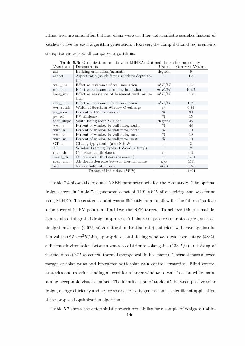
rithms because simulation batches of six were used for deterministic searches instead of

batches of five for each algorithm generation. However, the computational requirements

are equivalent across all compared algorithms.

Table 5.6: Optimization results with MIHEA: Optimal design for case studyVariable Description Units Optimal Valuesazi Building orientation/azimuth degrees 0aspect Aspect ratio (south facing width to depth ra-

tio)– 1.3

wall_ins Effective resistance of wall insulation m2K/W 8.93ceil_ins Effective resistance of ceiling insulation m2K/W 10.97base_ins Effective resistance of basement wall insula-

tionm2K/W 5.08

slab_ins Effective resistance of slab insulation m2K/W 1.39ovr_south Width of Southern Window Overhangs m 0.34pv_area Percent of PV area on roof % 90pv_eff PV efficiency % 15roof_slope South facing roof/PV slope degrees 45wwr_s Percent of window to wall ratio, south % 48wwr_n Percent of window to wall ratio, north % 10wwr_e Percent of window to wall ratio, east % 10wwr_w Percent of window to wall ratio, west % 10GT_s Glazing type, south (also N,E,W) – 2FT Window Framing Types (1:Wood, 2:Vinyl) – 2slab_th Concrete slab thickness m 0.2vwall_th Concrete wall thickness (basement) m 0.251zone_mix Air circulation rate between thermal zones L/s 133infil Natural infiltration rate ACH 0.025

Fitness of Individual (kW h) -1491

Table 7.4 shows the optimal NZEH parameter sets for the case study. The optimal

design shown in Table 7.4 generated a net of 1491 kWh of electricity and was found

using MIHEA. The cost constraint was sufficiently large to allow for the full roof-surface

to be covered in PV panels and achieve the NZE target. To achieve this optimal de-

sign required integrated design approach. A balance of passive solar strategies, such as:

air-tight envelopes (0.025 ACH natural infiltration rate), sufficient wall envelope insula-

tion values (8.56 m2K/W ), appropriate south-facing window-to-wall percentage (48%),

sufficient air circulation between zones to distribute solar gains (133 L/s) and sizing of

thermal mass (0.25 m central thermal storage wall in basement). Thermal mass allowed

storage of solar gains and interacted with solar gain control strategies. Blind control

strategies and exterior shading allowed for a larger window-to-wall fraction while main-

taining acceptable visual comfort. The identification of trade-offs between passive solar

design, energy efficiency and active solar electricity generation is a significant application

of the proposed optimization algorithm.

Table 5.7 shows the deterministic search probability for a sample of design variables146

from the case study. The search probability is defined as the probability that a given

design variable will be searched deterministically within the MIHEA. The probability of

selecting a variable for a deterministic search with no prior information is 1/N , where

N is the number of design variables. The actual search probability was calculated by

post-processing previous MIHEA optimization runs. The variables with the highest

deterministic search probability were the sizing of renewable energy generation, such

as PV efficiency, area of PV coverage, roof/PV slope and heating/cooling setpoints.

Variables that were rarely selected for deterministic searches were the solar orientation

of the building (azimuth) and the aspect ratio (ratio of south facing width to depth

ratio). Both variables were tightly coupled to other design variables. The optimization

of coupled variables is best handled in the EA.

Table 5.7: Search probability of design variable within MIHEA for Case StudyVariable Description Search Probability (%)

pv_eff PV efficiency 5.4pv_area PV area 5.3

roof_slope Roof and PV angle 5.1set_heat Heating setpoint 4.8set_cool Cooling setpoint 4.7aspect Aspect ratio 1.6

azi Building orientation 0.6

Box-whisker (BW) plots compared the distribution of optimization results for each

optimization algorithm (Fig. 5.3). BW plots allow for side-by-side comparisons of the

convergence characteristics of each algorithm using five important statistical properties

of the optimization datasets. In the BW plots, the dashes represent extremes of the data

points (starting point of initial population and final optimized population). The thick

line inside the box represents the mean quartile of the set. The lines of the box represent

the lower and upper quartiles of the set where 50% of data points reside. The algorithm

with the lowest mean fitness has the best convergence properties. Bean plots (Kampstra,

2008) were superimposed onto this Figure to show the individual fitness distribution

throughout the search using Gaussian kernel density functions (Scott, 1992). The three

dotted lines represent the global maximum, minimum and mean of the dataset. These

lines are intended to simplify visual comparison of results.

Figure 5.3 shows the convergence analysis results for the case study using 20 opti-

mization runs.

Both EA and MIHEA found better optimal designs and evolved more individuals147

PSOIWMontreal

EAMontreal

MIHEAMontreal

−150

041

0097

0015

000

global average global minimum global maximum

Search Algorithm and Location

Net

ann

ual e

lect

ricity

con

sum

ptio

n (k

Wh)

Figure 5.3: Box-whisker plot for 20 optimization runs

closer to the optimal landscape than the PSOIW. Note, the best individual from repeated

PSOIW optimization was close to the EA solution; however both EAs were able to

converge to the near-optimal landscape using fewer fitness evaluations which led to

surplus individuals, as illustrated by spiking in the distribution. Note that this spike

is absent in the PSOIW algorithm. MIHEA identified optimal solutions using only 22

generations compared to the 35 required by the proposed EA and PSOIW.

5.6 Conclusions

In this paper a hybrid evolutionary algorithm is proposed for minimizing solar building

energy consumption. A net-zero energy house was used as a case-study to demonstrate

the algorithm. Optimization approaches are required to identify cost-effective trade-offs

between passive solar design and renewable energy generation. The MIHEA algorithm

utilized information regarding variable interactions during the optimization process to

identify opportunities for deterministic searches. This augmentation is valuable as EAs

are strong at optimizing interdependent variables but have difficulties optimizing weakly

coupled design variables—a strength of deterministic searches. Results suggest that this

approach improves the reproducibility of near optimal solution set while requiring less

computational resources.

The proposed MIHEA algorithm is applicable to any problem that involves vari-

ous strengths of design variable interactions including several weakly interacting design

148

variables. Building energy simulation tools used for performance evaluations of solar

buildings, such as ESP-r or EnergyPlus, are ideal case studies as they involve solving

sets of sparse matrices (Clarke, 2001) or iterative solvers applied to loosely-coupled heat

balance equations (DOE, 2011b). However, the proposed algorithm may be useful for

other fields. Furthermore, using mutual information calculations to identify variables

that may be susceptible to deterministic searches is not specific to an evolutionary al-

gorithm. The approach could have equally been integrated into the PSOIW algorithm

or a different algorithm entirely.

The information gained using the proposed optimization strategy is applicable to

practicing energy modellers. For example, knowing which sets of design variables require

simultaneous tuning and which design variables can be selected in isolation is useful

information for energy modellers attempting to model high performance buildings.

149

Chapter 6

A Methodology for Identifying the

Influence of Design Variations on Building

Energy Performance

“Never again will scientific life be as satisfying and serene as in days whendeterminism reigned supreme. In partial recompense for the tears we must shedand the toil we must endure is the satisfaction of knowing that we are treatingsignificant problems in a more realistic and productive fashion.

–Richard Bellman ”“The greatest value of a picture is when it forces us to notice what we neverexpected to see.

–John Tukey ”6.1 Overview

In building performance simulation, understanding the potential for parameter vari-

ations to cause a disproportionately large change in a performance metric is an

important aspect of the modelling and design process. This is especially true if the

proposed building is expected to meet a performance target such as net-zero energy

consumption. This chapter proposes a methodology to identify influential variations

around a performance criterion. This methodology aids in the understanding of pos-

sible discrepancies between predicted and realized building performance. This chapter

uses the archetype solar home that combines passive solar design, energy efficiency mea-

sures including a geothermal heat pump and a building-integrated photovoltaic system150

proposed in chapter 4. The proposed methodology was accepted for publication with

revisions in the Journal of Building Performance Simulation (Bucking et al., 2013c).

6.2 Background

This chapter proposes a methodology to estimate the effect of variations around a perfor-

mance criterion. This methodology aids in the understanding of discrepancies between

predicted and realized building performance. A case-study demonstrates the method-

ology by identifying system level variations which significantly affect the net-energy

consumption of a NZEH. This information is useful to designers of NZE buildings wish-

ing to ensure that as-built designs equal or exceed preliminary performance estimates

from models. As discussed later, such information could be used to streamline quality

control processes.

The next section describes the methodology and a case study.

6.3 Methodology

This section proposes a methodology to estimate the effect of variations about a per-

formance criterion. In a later section, the methodology is used to identify system level

variations which most greatly affect the net-energy consumption of a NZEH.

To accomplish this, the methodology required the following distinct steps: (i) an

optimization training dataset was formed using an optimization algorithm, (ii) discrete

PDFs were created from this dataset for designs which satisfied the NZE performance

criterion, (iii) new designs were created from independent random samplings of these

PDFs and simulated using an objective function (due to system level effects, not all of

these samplings resulted in NZEHs), (iv) a back-tracking search identified the variations

responsible for non-NZE compliant samples.

Based on the literature review, presented in section 2.6.2, a MCA was selected for

uncertainty propagation. Based on the recommendations of Macdonald (2009), a ran-

dom sampling method was selected for the MCA to allow for an unbiased sampling of

the solution space. To explore influences of input variations for a performance criterion

such as NZE requires experimental evidence or expert knowledge. Associating arbitrary

151

PDFs to model inputs, such as normal or triangle distributions, offers no indication that

sampled designs represent or fall within the desired performance range. To overcome

this problem, optimization techniques extracted PDFs from the solution space of ac-

ceptable designs. Most of the sensitivity techniques used in literature were not suitable

to extract and rank the relative importance of variation combinations to model inputs

while retaining a performance criterion such as NZE. Based on the reviewed papers, only

Monte Carlo Filtering techniques using regression analysis met this restriction. How-

ever, Monte Carlo Filtering is only suitable to explore first order effects (Saltelli et al.,

2008). A back-tracking search, proposed in section 3.3.8.1, is used to explore first and

higher order effects.

The methodology is divided into three sections described by the following compo-

nents: (i) creation of optimization dataset using an Evolutionary Algorithm and ex-

traction of PDFs, (ii) a Monte Carlo analysis using samplings of discrete PDFs, and

(iii) importance factor calculations using back-tracking searches.

6.3.1 Formation of PDFs from an Optimization Training Dataset

This section describes the steps required to build PDFs from a training dataset built

using an optimization algorithm; this training dataset will be used within a MCA.

The steps, summarized in Figure 6.1, are as follows: (i) model formation, (ii) dis-

cretization of variables, (iii) formation of optimization training dataset using a cus-

tomized evolutionary algorithm (Bucking et al., 2010, 2013b), and (iv) extraction of

PDFs for each model variable from compliant designs in the optimization training

dataset. These steps are described in greater detail below.

Before proceeding, it is assumed that a model exists to evaluate the performance

criterion. Simulation of this model allowed for comparisons of design performance.

The methodology requires discrete variables. This step is beneficial as it improves

the convergence properties of the optimization algorithm. Furthermore, the resolution

of most variables in building applications is finite in application. Although continu-

ous parameters would result in higher resolution estimates of variability, they require

additional binning which is sensitive to bin size. Thus, the methodology requires that

appropriate design parameter increments be selected.

152

Run Optimization for M generations



Discretization of design variables

Model formation and selection ofdesign variables

(ex. window/wall ratio, insulation value)

…

Formation of Training Dataset:Select set of optimal designswhich equal, or exceed NZE

PROBABILITY DISTRIBUTION FUNCTIONS

…

…var1 var2 varN

Prob

Prob

Prob

Randomly Initiated Population #1

(size P)

Randomly InitiatedPopulation #2

(size P)

Randomly Initiated Population #N

(size P)

Figure 6.1: Formation of PDFs from the optimization dataset

In a MCA, attributing representative distributions with physical interpretations to

the input parameters of the model is difficult. There is no evidence that samplings

of common distribution functions such as normal or triangle distributions will repre-

sent a performance criterion or fall within a desired performance range. To overcome

this difficulty, a training dataset was utilized based on searches from an optimization

algorithm.

Optimization algorithms identify which sets of design parameters resulted in a NZEH.

The selection of the optimization tool will not affect the training dataset if: (i) the algo-

rithm can optimize large solution spaces involving interacting variables, and (ii) path-

ways leading to optimal regions can be queried from a database. For the case study,

an evolutionary algorithm (Bucking et al., 2010; Eiben and Smith, 2003) was selected

to navigate the design space. Training data was built by running the optimization tool,

starting with a randomly selected initial population, at least N times for M generations

using a population of P designs to approach optimal landscapes from different directions.

Wright and Alajmi (2005) suggested a population size, P , of 10 to 15 is appropriate for

most building simulation applications. The selection of the number of generations, M ,

153

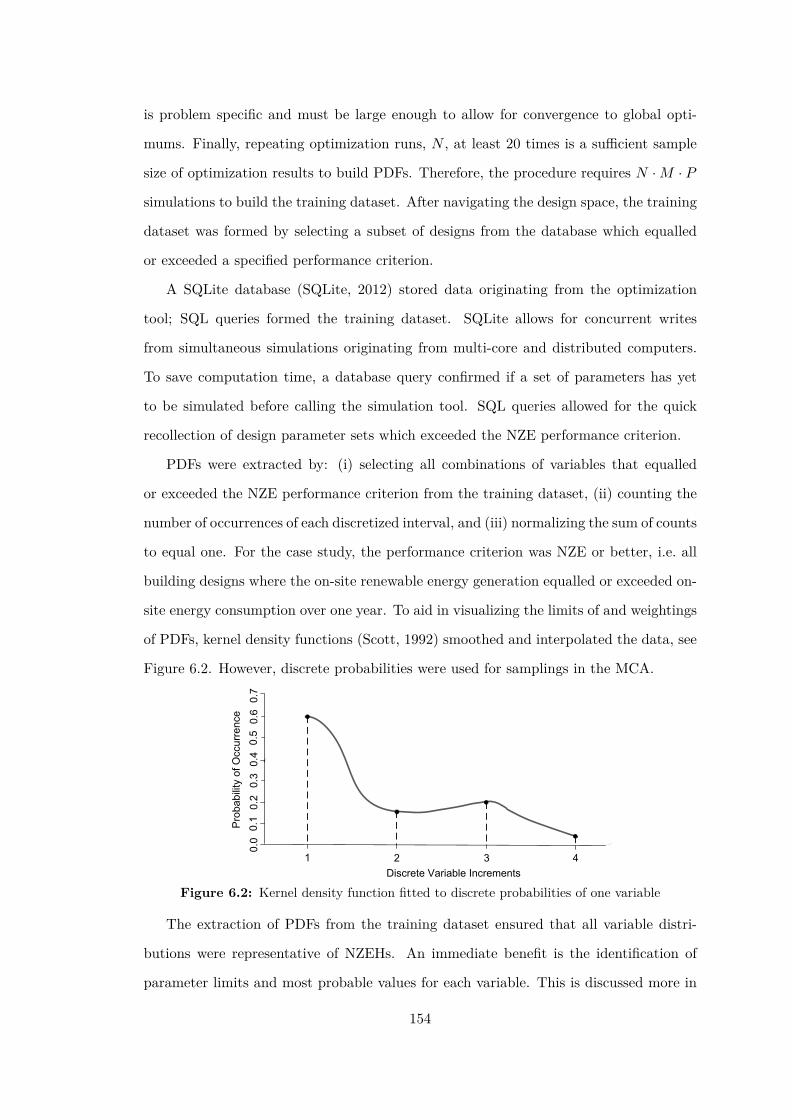
is problem specific and must be large enough to allow for convergence to global opti-

mums. Finally, repeating optimization runs, N , at least 20 times is a sufficient sample

size of optimization results to build PDFs. Therefore, the procedure requires N · M · P

simulations to build the training dataset. After navigating the design space, the training

dataset was formed by selecting a subset of designs from the database which equalled

or exceeded a specified performance criterion.

A SQLite database (SQLite, 2012) stored data originating from the optimization

tool; SQL queries formed the training dataset. SQLite allows for concurrent writes

from simultaneous simulations originating from multi-core and distributed computers.

To save computation time, a database query confirmed if a set of parameters has yet

to be simulated before calling the simulation tool. SQL queries allowed for the quick

recollection of design parameter sets which exceeded the NZE performance criterion.

PDFs were extracted by: (i) selecting all combinations of variables that equalled

or exceeded the NZE performance criterion from the training dataset, (ii) counting the

number of occurrences of each discretized interval, and (iii) normalizing the sum of counts

to equal one. For the case study, the performance criterion was NZE or better, i.e. all

building designs where the on-site renewable energy generation equalled or exceeded on-

site energy consumption over one year. To aid in visualizing the limits of and weightings

of PDFs, kernel density functions (Scott, 1992) smoothed and interpolated the data, see

Figure 6.2. However, discrete probabilities were used for samplings in the MCA.

1 2 3 4

0.0

0.1

0.2

0.3

0.4

0.5

0.6

0.7

Pro

babi

lity

of O

ccur

renc

e

Discrete Variable Increments

Figure 6.2: Kernel density function fitted to discrete probabilities of one variable

The extraction of PDFs from the training dataset ensured that all variable distri-

butions were representative of NZEHs. An immediate benefit is the identification of

parameter limits and most probable values for each variable. This is discussed more in

154

the results section. Logically, one expects the sampling of a set of trained PDFs to result

in a NZE compliant design since the PDFs were extracted from a population of NZE

compliant designs. However, due to variable couplings, this is not always true. This

became evident if the Monte Carlo samplings from trained PDFs resulted in some non-

NZE compliant designs. In fact, by intentionally sampling model variables as though

they were independent variables indirectly identifies non-linear effects and inter-variable

interactions which cause non-NZE compliant designs.

The optimization dataset offered many insights into variations which caused a per-

formance criterion to be exceeded. Using the trained PDFs as an input, a Monte Carlo

analysis enabled the exploration of model variations around this performance criterion.

6.3.2 Monte Carlo Analysis

A Monte Carlo analysis was selected to identify the global effects of variations on the

previously defined PDFs. A MCA does not require modifications to the model and

can directly use the trained PDFs from the optimization training dataset for samplings.

Monte Carlo analyses are commonly referred to as uncertainty analyses since they esti-

mate the cumulative effect of sampling uncertain input distributions. For this chapter,

a MCA conducts a variability study since the input distributions represent parameter

sets of NZE buildings and not physical uncertainties in model inputs.

Figure 6.3 summarizes the steps required to estimate the global variability of a

model. A random sampling technique of trained PDFs was used for the MCA, based

on the recommendations of previous studies comparing sampling methods (Lomas and

Eppel, 1992; Macdonald, 2009). This methodology used sample sizes of 1000—ten times

more than the recommended sample size to estimate mean and variance of the outcome

distribution (Macdonald, 2009). Larger sample sizes helped to explore the effect of

sample size on importance factor convergence as discussed in section 6.3.3. In a MCA,

larger sample sizes tend to yield more normal distributions, due to the central limit

theory of statistics. Otherwise, they do not affect Monte Carlo outcomes.

Monte Carlo methods rely on the sampling of predefined input distributions to es-

timate the cumulative variability of a model. Data points are formed by simulating

samplings using a performance objective. The binning of all sampled data points forms

155

...

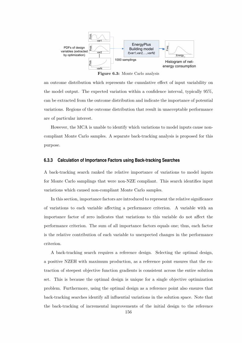
PDFs of designvariables (extracted

by optimization)

EnergyPlusBuilding modelf(var1,var2,…,varN)

Histogram of net-energy consumption

1000 samplingsEnergy

Prob

Pro

bP

rob

Freq

var1

var2

varN

Figure 6.3: Monte Carlo analysis

an outcome distribution which represents the cumulative effect of input variability on

the model output. The expected variation within a confidence interval, typically 95%,

can be extracted from the outcome distribution and indicate the importance of potential

variations. Regions of the outcome distribution that result in unacceptable performance

are of particular interest.

However, the MCA is unable to identify which variations to model inputs cause non-

compliant Monte Carlo samples. A separate back-tracking analysis is proposed for this

purpose.

6.3.3 Calculation of Importance Factors using Back-tracking Searches

A back-tracking search ranked the relative importance of variations to model inputs

for Monte Carlo samplings that were non-NZE compliant. This search identifies input

variations which caused non-compliant Monte Carlo samples.

In this section, importance factors are introduced to represent the relative significance

of variations to each variable affecting a performance criterion. A variable with an

importance factor of zero indicates that variations to this variable do not affect the

performance criterion. The sum of all importance factors equals one; thus, each factor

is the relative contribution of each variable to unexpected changes in the performance

criterion.

A back-tracking search requires a reference design. Selecting the optimal design,

a positive NZEH with maximum production, as a reference point ensures that the ex-

traction of steepest objective function gradients is consistent across the entire solution

set. This is because the optimal design is unique for a single objective optimization

problem. Furthermore, using the optimal design as a reference point also ensures that

back-tracking searches identify all influential variations in the solution space. Note that

the back-tracking of incremental improvements of the initial design to the reference156

design is equivalent to the back-tracking of incremental degradations of the reference

design to the initial design.

Figure 6.4 shows the method for calculating importance factors using back-tracking

searches. Designs of interest, shown as shaded region in histogram, refers to candidate

building designs for the back-tracking searches, i.e. designs which are non-NZE com-

pliant. To calculate importance factors, using each design of interest (j = 1, · · · , M):

(a) perform a back-tracking search from the design of interest to the reference building

to identify steepest performance gradients and incremental performance improvements

for each variable change; (b) calculate local importance factors by dividing the incre-

mental objective function gradient of each variable (Egrad i,j where i = 1, · · · , N) by the

difference in the objective functions between the design of interest (EDOI) and the refer-

ence building design (ERef ), see equation 6.1; (c) continue to the next design of interest

and repeat from step (a) until all non-NZE compliant designs have been back-tracked;

finally, (d) calculate and rank global importance factors by normalizing all local impor-

tance factors calculated in steps (a–c), see equation 6.2. The sum of global importance

factors for all variables should be equal to one. These factors are global in the sense that

they represent the average effect of variations on non-compliant Monte Carlo samples.

IFlocal i,j = Egrad i,j

EDOI − ERef(6.1)

IFglobal i =∑

j IFlocal i,j∑i

∑j IFlocal i,j

where,∑

i

IFglobal i = 1 (6.2)

Histogram of net-energyconsumption (from MCA)

Designs ofInterest

Back-trackingsearch of designs

of interest

Design of interest 1

var1 var2 var3 ...

Design of interest N

var3 var2 var1 ...

…

Note, sum(Importance)=1

var1 var3 var2 ...

Impo

rtanc

eFr

eq

Ene

rgy

Ene

rgy

Energy

Ref.Design

Ref.Design

PerformanceCriterion

Calculate local importance factors

Normalize and average

local importance factors

Global ImportanceFactors

energydecrements

energydecrements

Figure 6.4: Calculation of importance factors using back-tracking searches

157

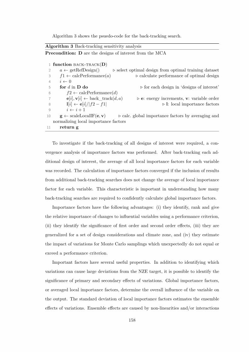
Algorithm 3 shows the psuedo-code for the back-tracking search.

Algorithm 3 Back-tracking sensitivity analysisPrecondition: D are the designs of interest from the MCA

1 function back-track(D)2 a ← getRefDesign() � select optimal design from optimal training dataset3 f1 ← calcPerformance(a) � calculate performance of optimal design4 i ← 05 for d in D do � for each design in ‘designs of interest’6 f2 ← calcPerformance(d)7 e[i], v[i] ← back_track(d, a) � e: energy increments, v: variable order8 l[i] ← e[i]/|f2 − f1| � l: local importance factors9 i ← i + 1

10 g ← scaleLocalIF(e, v) � calc. global importance factors by averaging andnormalizing local importance factors

11 return g

To investigate if the back-tracking of all designs of interest were required, a con-

vergence analysis of importance factors was performed. After back-tracking each ad-

ditional design of interest, the average of all local importance factors for each variable

was recorded. The calculation of importance factors converged if the inclusion of results

from additional back-tracking searches does not change the average of local importance

factor for each variable. This characteristic is important in understanding how many

back-tracking searches are required to confidently calculate global importance factors.

Importance factors have the following advantages: (i) they identify, rank and give

the relative importance of changes to influential variables using a performance criterion,

(ii) they identify the significance of first order and second order effects, (iii) they are

generalized for a set of design considerations and climate zone, and (iv) they estimate

the impact of variations for Monte Carlo samplings which unexpectedly do not equal or

exceed a performance criterion.

Important factors have several useful properties. In addition to identifying which

variations can cause large deviations from the NZE target, it is possible to identify the

significance of primary and secondary effects of variations. Global importance factors,

or averaged local importance factors, determine the overall influence of the variable on

the output. The standard deviation of local importance factors estimates the ensemble

effects of variations. Ensemble effects are caused by non-linearities and/or interactions

158

with other variables. An importance factor with a large variance indicates that the effect

of variations is strongly affected by the values of other parameters. By contrast, low

values imply that the effect is almost independent of other sampled parameters. Note

that primary effects are de-emphasized in this methodology since back-tracking searches

are intentionally conducted on designs with sufficient system-level interactions to cause

non-NZE building designs. Similar to the Morris method (Morris, 1991), the mean and

standard deviation of importance factors can be plotted against each other to visualize

primary and secondary effects.

The following section presents a case study to demonstrate the proposed methodol-

ogy.

6.4 Case Study

The proposed methodology was applied using an energy model described in chapter 3.

The archetype solar building design presented previously in chapter 4 was used for the

case-study. This case study used twenty-six discrete variables, summarized in Table 6.1.

Note that some variables may depend on circumstances which the designer might not

have control over such as construction air-tightness, orientation and occupant behaviour.

Variable descriptions are shown for the south orientation only; also, the PV slope is equal

to the roof slope since the house has a building-integrated photovoltaic system that

covers the south-facing roof. The performance objective selected was the net-annual

electricity consumed (Net) during a typical meteorological year, i.e. the energy balance

of building energy consumption with renewable energy (RE) generation, see equation 6.3.

Negative values of net-energy indicate a greater production of electricity compared to

consumption. Thus, satisfying or exceeding the NZE criterion can be stated succinctly

as Net ≤ 0 or RE ≥ Consumption.

Net = Consumption − RE (6.3)

An evolutionary algorithm minimized the annual net-energy consumption of the

house. The algorithm used a population size P of 10 with 30 generations (M) within each

optimization run. To ensure that the optimal landscape was approached from different

159

Table 6.1: Sample of influential model variables for a NZEH

Variable Units Min. Max. No. Steps Description

aspect – 0.7 2.2 16 Aspect ratio (south facing width to depth ratio)azi degrees -45 45 32 Building orientation/azimuthwall_ins m2K/W 3.5 13.0 8 Effective resistance of wall insulationceil_ins m2K/W 5.6 15.0 8 Effective resistance of ceiling insulationbase_ins m2K/W 0.0 7.0 8 Effective resistance of basement wall insulationslab_ins m2K/W 0.0 2.3 4 Effective resistance of slab insulationheating_sp ◦C 18 25 4 Heating setpointcooling_sp ◦C 25 28 4 Cooling setpointinfil ACH 0.025 0.179 8 Natural infiltration rateocc_loads % CADavg 50 80 8 Occupant loads (percent of Canadian average consumption)ovr_south m 0.00 0.45 4 Width of Southern Window Overhangspv_area % 0 90 8 Percent of PV area on roofpv_eff % 12 15 4 PV efficiencyroof_slope degrees 30 47 8 South facing roof/PV slopewwr_s % 5 80 8 Percent of window to wall ratio, south (also N,E,W)GT_s – 1 4 4 Glazing type, south (also N,E,W)FT – 1 2 2 Window Framing Types (1:Wood, 2:Vinyl)slab_th m 0.1 0.2 8 Concrete slab thicknessvwall_th m 0.00 0.35 8 Concrete wall thickness (basement)zone_mix L/s 0 400 4 Air circulation rate between thermal zones

angles, 20 optimization runs (N) were executed using randomized initial populations;

thus, 6000 EnergyPlus simulations were required (P · M · N = 6000). Approaching the

optimal landscape from different pathways ensured that the extracted PDFs represented

a variety of interactions present in the building model.

6.5 Results

Figure 6.5 shows the PDFs extracted from the optimization training set. Table 6.1

provides longer descriptions of short-form notations. The probabilities of each variable,

shown in the y-axis, are normalized to one.

Each PDF resulted in a NZE compliant design given a specific set of other variable

combinations. Two-dimensional contour maps are more appropriate to visualize discrete

combinations of variables that resulted in NZE compliant designs. For example, Fig-

ure 6.6 shows a probability contour plot, based on several near-optimal designs from

the training dataset, for the southern window glazing to wall ratio (WWR) and for the

amount of wall insulation. The shaded region shows variable combinations that resulted

in a NZE compliant home for this particular case study (RE ≥ Consumption). Shading

indicates the probability that the combination of parameters appeared in the training

dataset; darker shading indicates an increased probability of occurrence.

160

50 55 60occ_loads [% CAD_avg]

72 74 76 78 80pv_area [%]

38 42 46 50roof_slope [degrees]

16 18 20 22 24heating_sp [degC]

0 20 40 60 80wwr_s [%]

40 0 20 40azi [degrees]

0.00 0.10 0.20infil [ACH]

0.5 1.5 2.5aspect [ ]

13.8 14.2 14.6 15.0pv_eff [%]

4 6 8 12 16wall_ins [m2 K/W]

0 10 20 30 40wwr_n [%]

24 25 26 27 28 29cooling_sp [degC]

0 10 20 30 40wwr_e [%]

0 10 20 30 40wwr_w [%]

0.0 0.2 0.4 0.6ovr_south [m]

0.0 0.1 0.2 0.3 0.4vwall_th [m]

Figure 6.5: Sample of PDFs extracted from the training dataset

0.00

0.01

0.02

0.03

0.04

0.05

0.06

5.0 15.7 26.4 37.1 47.9 58.6 69.3 80.0

3.5

4.9

6.2

7.6

8.9

10.3

11.6

13.0

wwr_s [%]

wal

l_in

s [m

2 K

/W]

Probability

Figure 6.6: Probability of occurrence for southern WWR and wall insulation parameters re-sulting in homes that are NZE compliant

One important observation from Figure 6.6 is that some combinations of wall in-

sulation and WWR preferentially appeared in clusters due to coupling; for example, a

range of southern WWRs of 31.8–47.9% correlated with wall insulation levels of 6.9–8.3

m2K/W indicating that these variable pairings has a high probability of occurrence in

the NZEH training dataset. Additional pairings can be found for higher wall insula-

tion and lower southern WWRs. This important result demonstrates two very different

approaches to design a NZEH: (i) super insulated walls with more variable southern

WWR, and (ii) a design with relatively lower wall insulation and appropriately sized

southern WWR for passive solar design. Both are valid design strategies to achieve the

NZE performance criterion. This result quantifies these two different approaches that

161

until now were described qualitatively: super insulate and be conservative in window

areas versus insulate well—but not excessively—and use larger window areas. The sec-

ond approach was used in the design of the ÉcoTerra house, but the first approach

was used in some of the other EQuilibrium houses.

Once the PDFs were extracted from the optimized training dataset, a MCA was

performed which resulted in a histogram of the accumulated effects of design varia-

tions, as shown in Figure 6.7. If all variables were weakly interacting, the sampling of

trained PDFs from NZE compliant design in a MCA would result in all NZE compli-

ant design. However, the shaded area in Figure 6.7 identifies designs where renewable

energy generation did not offset the building energy consumption. This is due to vari-

able interactions and non-linearities. The histogram satisfied a hypothesis test for a

long-tail distribution (Venables and Ripley, 2002). Long-tailed distributions represent

rare events—meaning that deviations from NZE require more than one variable change.

The back-tracking analysis proposed, described in section 6.3.3, identifies the variations

responsible for long-tail events.

If one was to approximate a mean and variance, assuming a normal distribution,

the expected net annual electricity consumption given all variations would be −400 ±850 kWh using a 95% confidence interval. Negative values of energy indicate the net-

production of electricity. For this case study, the combined variations is enough to cause

building energy consumption to be larger than renewable energy generated in 20.4%

(204/1000) of sampled designs, i.e. RE < Consumption.

Net annual electricity consumption (kWh)

Num

ber o

f bui

ldin

g de

sign

s

−1500 −1000 −500 NZE 500 1000 1500

060

120

Designs of Interest: i.e. Designs where RE<Consumption

(204 sampled designs)

Figure 6.7: Histogram of 1000 samples from the Monte Carlo analysis

Importance factors were calculated for input variables responsible for NZE non-

compliance. As shown in Figure 6.7, 20.4% of the sample was non-NZE compliant. Im-

162

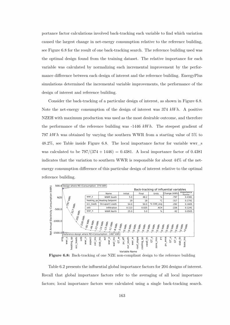
portance factor calculations involved back-tracking each variable to find which variation

caused the largest change in net-energy consumption relative to the reference building,

see Figure 6.8 for the result of one back-tracking search. The reference building used was

the optimal design found from the training dataset. The relative importance for each

variable was calculated by normalizing each incremental improvement by the perfor-

mance difference between each design of interest and the reference building. EnergyPlus

simulations determined the incremental variable improvements, the performance of the

design of interest and reference building.

Consider the back-tracking of a particular design of interest, as shown in Figure 6.8.

Note the net-energy consumption of the design of interest was 374 kWh. A positive

NZEH with maximum production was used as the most desirable outcome, and therefore

the performance of the reference building was -1446 kWh. The steepest gradient of

797 kWh was obtained by varying the southern WWR from a starting value of 5% to

48.2%, see Table inside Figure 6.8. The local importance factor for variable wwr_s

was calculated to be 797/(374 + 1446) = 0.4381. A local importance factor of 0.4381

indicates that the variation to southern WWR is responsible for about 44% of the net-

energy consumption difference of this particular design of interest relative to the optimal

reference building.

ori

g

ww

r_s

heati

ng_s

p

occ

_loads

infil

ww

r_n

asp

ect

ceil_

ins

slab_i

ns

azi

ww

r_e

wall_

ins

GT_w

pv_e

ff

ovr_

south

ww

r_w

roof_

slope

coolin

g_s

p

vw

all_

th

GT_s

zone_m

ix FT

pv_a

rea

GT_n

GT_e

slab_t

h

base

_ins

Variable Name

-1500.0

-1000.0

-500.0

NZE

500.0

Net

Annual Ele

ctri

city

Consu

mpti

on (

kWh) Design where RE<Consumption: 374 kWh

Reference design where RE>Consumption: -1467 kWh

-797 kWh

-317 kWh

-292 kWh

-226 kWh

-92 kWh

-46 kWh

-23 kWh

-13 kWh

-13 kWh

-11 kWh

-8 kWh

-3 kWh

0 kWh

0 kWh

0 kWh

0 kWh

0 kWh

0 kWh

0 kWh

0 kWh

0 kWh

0 kWh

0 kWh

0 kWh

0 kWh

0 kW

h

Name Initial Final Units Change (kWh) ImportanceFactor

wwr_s WWR South 5.0 48.2 % -797 0.4381

heating_sp Heating Setpoint 19 18 °C -317 0.1741

occ_loads Occupant Loads 54.0 50.0 % CAD_avg -292 0.1605

infil Infiltration 0.113 0.025 ACH -226 0.1241

wwr_n WWR North 25.0 5.0 % -92 0.0505

Back-tracking of influential variables

Figure 6.8: Back-tracking of one NZE non-compliant design to the reference building

Table 6.2 presents the influential global importance factors for 204 designs of interest.

Recall that global importance factors refer to the averaging of all local importance

factors; local importance factors were calculated using a single back-tracking search.

163

The average net-change presented in this table is the expected change in net-energy

consumption found in the back-tracking search for all 204 designs.

Table 6.2: Importance factors for influential variables

Variable Units DescriptionMean

ImportanceFactor

ImportanceFactor

Deviation

AverageNet-Change

(kWh)

occ_loads % CADavg Occupant Loads (percentage of Cana-dian Average consumption)

0.1420 0.1258 253

pv_area % Percent area of PV on roof 0.1104 0.1490 200roof_slope % Roof slope 0.1043 0.1627 197heating_sp ◦C Heating setpoint 0.0993 0.1233 182

wwr_s % Percent of window to wall ratio, south 0.0868 0.1280 154azi degrees Building orientation/azimuth 0.0828 0.1200 150infil ACH Natural infiltration rate 0.0705 0.0931 129

pv_eff % PV efficiency 0.0445 0.1238 82

Table 6.2 is applicable to other NZEHs with similar variables, RE generation tech-

nology, site and situational constraints and climate type as the case study. For different

studies, users should repeat the proposed methodology. Calculating the effect of com-

binations of variations is achieved by adding the average net-changes. This linear as-

sumption may approximate some local non-linear phenomena but is generally acceptable

since net-changes originated from the solution space.

Figure 6.9 shows a plot of importance factor mean and standard deviation. Re-

call that the mean importance factor represents the overall influences of each variable

on the non-compliant MC samples shown in Figure 6.7. The importance factor stan-

dard deviation represents the effect of non-linearities or inter-variable couplings of each

variable. This figure shows three clusters of importance factors: (i) cluster A called in-

fluential variables, (ii) cluster B, variables with intermediate influence, and (iii) cluster

C, non-influential variables. Based on this plot, only 8 of the 26 variables examined were

considered influential.

Figure 6.10 shows the convergence characteristics for the five most influential vari-

ables over the back-tracked home designs found to greatly influence the NZE objective.

It was found that the calculation of importance factors converged after back-tracking

approximately 150 of the 204 building designs. For instance, the value at 50 building

designs is the average importance factor calculated for back-tracked building design no. 1

through no. 50. Similarly, the value at 100 building designs is the average of importance

factor from design no. 1 through no. 100.164

0.00 0.02 0.04 0.06 0.08 0.10 0.12 0.14

0.00

0.05

0.10

0.15

Mean Importance Factor

Sta

ndar

d D

evia

tion

of Im

port

ance

Fac

tors

pv_eff heating_sp

wall_ins

ovr_south

infil

wwr_e

wwr_w

aspectwwr_n

roof_slope

base_ins

wwr_s

cooling_sp

azi

vwall_thGT_s

pv_area

occ_loads

Cluster A:In uential Variables

Cluster B:Variables with some e ect

Cluster C:Non-in uentialVariables

Figure 6.9: Plot of importance factor mean and standard deviation

Figure 6.10: Convergence characteristics for the five most influence variables towards a constantimportance factor

6.6 Discussion and Conclusion

This chapter proposed a methodology to identify influential variations around a perfor-

mance criterion. A net-zero energy house case-study demonstrated the methodology.

Although the methodology is catered towards NZE buildings, it is applicable to other

high performance building studies. The remainder of this section discusses results from

the case study and areas of future work.

The application of the methodology to a NZEH identified several design restrictions

specific to the case study. From the set of PDFs shown in Figure 6.5, limits in variable

ranges that resulted in NZE were identified. For instance, if occupants consumed more165

than 60% of Canadian national electricity averages for appliance, DHW and lighting

loads, achieving NZE was not practically possible, i.e. PDFs equalled zero. Other similar

design restrictions were noted for the building azimuth angle and PV sizing. For example,

NZE compliance is difficult to achieve when the main solar collecting surface of the

building is oriented greater than 30 degrees of south. Note that these results are for

a particular location and a set of modelling assumptions but they are expected to be

valid for similar climatic conditions. For this case study, cut-offs originated due to a

limited amount of roof space for PV-based electricity generation. Regardless, Figure 6.5

shows a remarkable variety of design combinations with the potential to reach NZE.

Figure 6.6 identified that some combinations of wall insulation and WWR preferentially

appeared in clusters. For example, a range of southern WWRs of 31.8–47.9% correlated

with wall insulation levels of 6.9–8.3 m2K/W . This result represents two very different

design approaches to a NZEH: (i) super insulated walls with more variable southern

WWR, and (ii) a design with relatively lower wall insulation and appropriately sized

southern WWR for passive solar design. Identifying variable restrictions and optimal

combinations of variations in the early design stages of a NZE building will facilitate the

quantitative design process.

The convergence of importance factors exhibited an asymptotic relationship regard-

less of the order of the back-tracked population (see Figure 6.10). The convergence

analysis indicated that at least at least 150 back-tracking searches were required to

build confident estimates of global importance factors.

In the case study, importance factors indicated that only a few design variables as-

sociated with a NZEH significantly affect net-energy consumption. In fact, only thirty

percent of the variables examined in the case study were influential. Energy related

occupant behaviour (occ_loads) was the most influential variable. Occupant behaviour

carried more significance than design variations affecting heating and cooling loads due

to the COP effect of the heat pump which reduced electricity used by 1/COP. Monitored

data from a set of NZEHs would be more appropriate to extract the importance of occu-

pant behaviour. For this study, ranges of occupant behaviour were based on monitored

data of a NZEH and average energy consumption data for Canada. Since the occ_loads

importance factor was based on these assumptions of occupant behaviour, these results

166

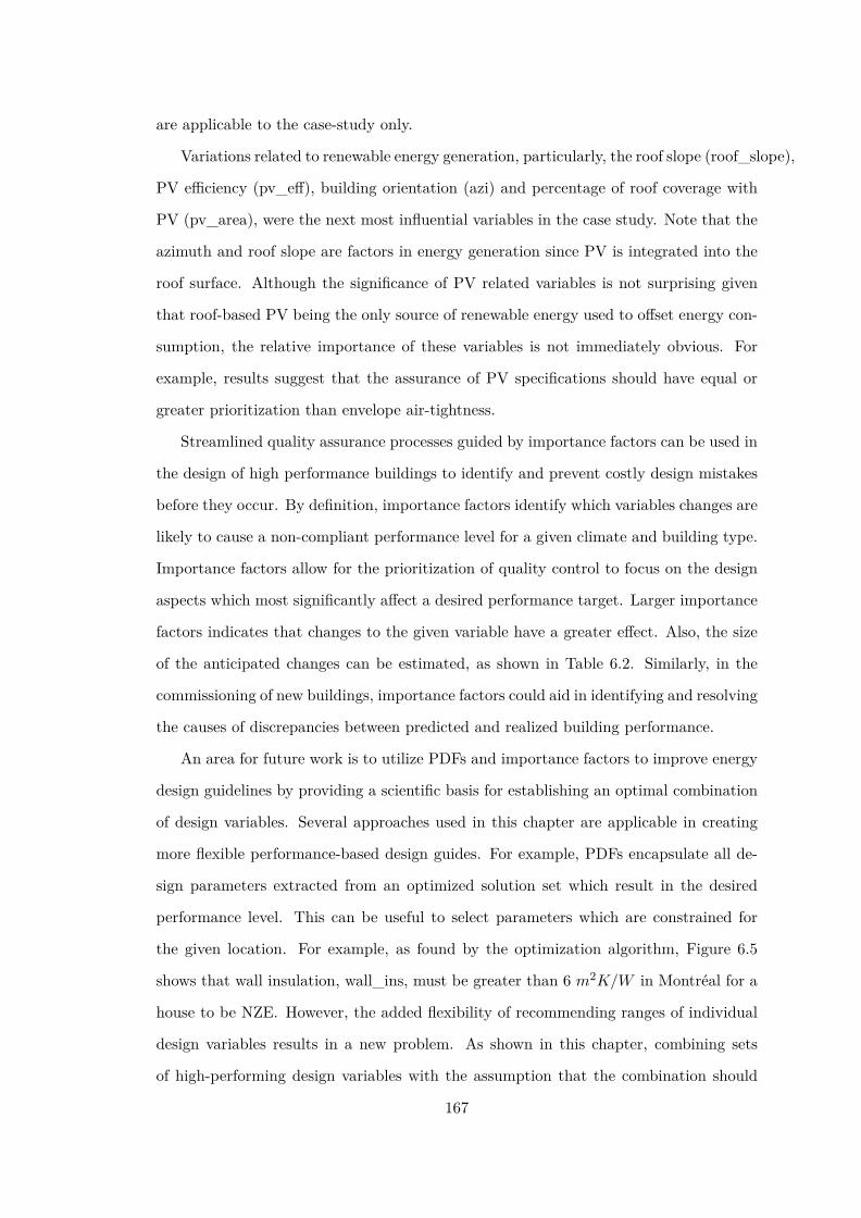
are applicable to the case-study only.

Variations related to renewable energy generation, particularly, the roof slope (roof_slope),

PV efficiency (pv_eff), building orientation (azi) and percentage of roof coverage with

PV (pv_area), were the next most influential variables in the case study. Note that the

azimuth and roof slope are factors in energy generation since PV is integrated into the

roof surface. Although the significance of PV related variables is not surprising given

that roof-based PV being the only source of renewable energy used to offset energy con-

sumption, the relative importance of these variables is not immediately obvious. For

example, results suggest that the assurance of PV specifications should have equal or

greater prioritization than envelope air-tightness.

Streamlined quality assurance processes guided by importance factors can be used in

the design of high performance buildings to identify and prevent costly design mistakes

before they occur. By definition, importance factors identify which variables changes are

likely to cause a non-compliant performance level for a given climate and building type.

Importance factors allow for the prioritization of quality control to focus on the design

aspects which most significantly affect a desired performance target. Larger importance

factors indicates that changes to the given variable have a greater effect. Also, the size

of the anticipated changes can be estimated, as shown in Table 6.2. Similarly, in the

commissioning of new buildings, importance factors could aid in identifying and resolving

the causes of discrepancies between predicted and realized building performance.

An area for future work is to utilize PDFs and importance factors to improve energy

design guidelines by providing a scientific basis for establishing an optimal combination

of design variables. Several approaches used in this chapter are applicable in creating

more flexible performance-based design guides. For example, PDFs encapsulate all de-

sign parameters extracted from an optimized solution set which result in the desired

performance level. This can be useful to select parameters which are constrained for

the given location. For example, as found by the optimization algorithm, Figure 6.5

shows that wall insulation, wall_ins, must be greater than 6 m2K/W in Montréal for a

house to be NZE. However, the added flexibility of recommending ranges of individual

design variables results in a new problem. As shown in this chapter, combining sets

of high-performing design variables with the assumption that the combination should

167

result in a high performing design is circumstantial due to influential variable linkages

and couplings. Importance factors, by definition, identify which design variable changes

are responsible for such discrepancies. From the perspective of a design guide, the

smaller the importance factor of a design variable, the more confidently it can be used

in combination with other design variables.

The presented methodology is directly transferable to multiple objectives such as

life-cycle cost or embodied energy. The database query requires an additional lower or

upper bound for each additional performance objective.

It is likely that annual climatic variations such as variations in solar radiation, exte-

rior wind speed and air temperature will also affect the energy performance of a NZEH.

By including climatic factors, the proposed methodology can be applied to establish if

the building model, used to inform design decisions, represents the monitored energy op-

erations of the building. If the monitored energy consumption of the building falls within

the estimated uncertainty ranges while considering variations in occupant behaviour, de-

sign variations and climatic factors, the building is compliant with preliminary energy

models. The ability to determine if a predicted building model represents the operations

of a building also has implications toward building rating systems, retro and on-going

commissioning of buildings, and NZE building compliance checking. These topics will

be explored in future research.

168

Chapter 7

Optimization Methodology to Evaluate the

Effect Size of Incentives on Life-Cycle Cost

for NZEHs

“But humankind has a great capacity for finding technological solutions toseemingly intractable problems, and this will likely be the case for global warming.It isn’t that the problem isn’t potentially large. It’s just that humaningenuity—when given proper incentives—is bound to be larger. Even moreencouraging, technological fixes are often far simpler, and therefore cheaper, thanthe doomsayers could have imagined.

–Steven D. Levitt, SuperFreakonomics ”7.1 Overview

This chapter proposes a methodology to compare the effect of various incentives on

optimized building design. The goal of the methodology is to identify incentives

structures which improve the economics of performance-optimized building design. The

best incentive structures are further investigated in the next chapter. This methodology

was presented at an International conference on building simulation (Bucking et al.,

2013d).

169

7.2 Background

The adoption of net-zero energy buildings, like any new technology, is inhibited by cost.

An initial cost premium for a NZEB is expected due to the higher initial costs associ-

ated with balancing on-site energy generation against energy conservation and efficiency

measures. Essentially, NZEB owners pre-purchase their future energy needs before occu-

pying the building. Undoubtedly, there is motivation to move towards high performance

buildings due to dwindling fossil fuel reserves and climate change, as well as the superior

comfort and low operating costs these buildings provide. Given that it is technologi-

cally feasible to achieve NZEBs in most climates (Voss and Musall, 2012), perhaps, the

factor limiting the wide-spread adoption of NZEBs is the capacity of consumers to man-

age higher upfront costs. Economists see such stalemates as perfect opportunities for

economic incentives.

In Canada, the cost premium for specialized material and equipment of a net-zero

energy home (NZEH) is thought to be between $50,000–90,000 depending on loca-

tion (CMHC, 2008). Leckner (2008) suggested a NZEH in Montréal had an initial

cost premium of $34,300 (excluding solar energy generation) over a typical house, con-

structed in 1994, and achieved cost payback after 37 years; the embodied energy had a

payback of 8.4 years. Patil (2010) indicated that a NZEH in Montréal achieved embod-

ied energy payback after 9 years for PV, 7 years for PV/T and cost payback (including

solar energy generation) within a 50 year time horizon. This research indicated that

embodied energy payback is relatively short compared to life-cycle cost payback.

If the immediate target of NZE for buildings is too ambitious, then what performance

target is economically attractive? Can incentives be developed to encourage the tran-

sition towards a NZE building stock? What is the relationship between a cost-optimal

building and an energy-optimal building? This chapter examines the opportunity for

economic incentives to establish pathways towards cost-optimal NZEBs. It also further

develops key concepts from previous cost and energy optimization research.

The BEOpt development team proposed “swoosh” curves to represent cost-optimal

improvements relative to a Building America reference building (DOE, 2010), see Fig-

ure 7.1.

170

Figure 7.1: Energy-cost optimal curves in BEOpt (modified from Christensen et al. (2004))

The BEOpt team utilized a cost-optimization technique which identified all interme-

diate designs starting from a reference building to a cost optimal design and eventually a

NZEH (Christensen et al., 2004). BEOpt optimal cost curves, shown in Figure 7.1, have

several interesting features. The reference building, intended to represent the present

housing stock, is marked by point (A). Several design improvements can be made to

this reference design to identify a cost-optimal point, the most economically attrac-

tive building design, shown by point (B). The sequential search used always prioritizes

cost-improvements over energy performance improvements (Horowitz et al., 2008). The

transition point (C), is the point where energy generation becomes more cost effective

than improvements to energy efficiency and energy conservation. To attain the NZE

performance target, point (D), from the transition point (C), a specified number of PV

panels are used. The line from point (C) to point (D) is straight due to a linear cost

assumption of PV panel costs.

This energy-cost optimal curve has also appeared in European building performance

targets. In 2009, EU nations set a target that all new buildings should be NZE after

2020. One peculiarity in establishing this ambitious target is that no clear definitions

were given regarding what a NZEB was. Furthermore, no practical guidance was given

on how designers and contractors could achieve this target. It was later through the

energy performance building directive recast that a firm definition of the NZEB target

171

Primary Energy Consumption [kWh/m2]

GlobalCost[€/m2]

di erence in energy consumption di erence in energy consumption

optimum optimumcost neutral

reference referencedi erence in cost

Figure 7.2: Identification of cost optimal and cost neutral buildings (modified from BPIE(2010))

was formed (Kurnitski et al., 2011). The EU now mandates that all new buildings should

be nearly net-zero energy (nNZEB) after 2020 (EU Parliament, 2010). A nNZEB is

the cost-optimal building using a life-cycle cost analysis on the optimized pathway to

a NZEB, see Figure 7.2 (BPIE, 2010). The reference building suggested is defined

in EN15316-1 (2007). The nNZEB performance target is less ambitious and favours

cost-feasibility to dictate design. Regardless, optimization approaches are influential in

forming energy-cost optimal curves.

The Building Performance Institute Europe (BPIE) recommended that designers

pursue cost neutral or cost equivalent designs, see Figure 7.2. A cost neutral design has

similar life-cycle costs but resides on opposing limit of energy use intensity reductions on

the energy-cost optimal curve. They found that economic optimums involved a minor

reduction in energy use intensity (EUI) and cost compared to present energy standards.

To encourage further reductions in EUI, it was recommended that new buildings be cost

neutral with present standards. This means that a given building should be no more

expensive, using a life-cycle analysis, than the reference building but have significantly

reduced energy consumption. Reference buildings can be a particular energy code or

customized to represent a particular building stock. Although it has not been discussed

in literature, it is possible that economic incentives may positively effect energy-cost

curves.

The remaining chapter presents a methodology for identifying incentive opportunities

which create cost-optimal pathways towards NZEB design.

172

7.3 Method: Evaluating in Effect Size of Incentives on NZEH Design Opti-

mization

This section proposes a methodology to evaluate the effect of several financial incentives

on cost-optimal pathways towards NZEBs. In addition, the relationship between cost

and energy optimized buildings are examined. To accomplish these goals, the energy-cost

curves introduced in the previous section measured the effect of incentives. The following

incentive types are explored: (i) incentives which reduce the initial cost premium of a

NZEH; (ii) incentives which create revenue streams for part of the life-cycle period;

and (iii) disincentives to a typical reference building which indirectly incent the NZE

objective.

The proposed methodology and results build from the tools and design concepts

presented in previous chapters. To exemplify the approach, a NZEH located in Mon-

tréal, as described in section 3.4 was used. Two objective functions are used. Objective

function 1 (obj. 1) is the net-energy consumption described by equation 3.13 in sec-

tion 3.4. Objective function 2 (obj. 2) is the life-cycle cost described by equation 3.17

in section 3.5.

To identify the effect of incentives on pathways towards NZEBs, several objectives

are identified: (i) formation of a reference building; (ii) creation of energy-cost per-

formance curve using no incentives (base case); (iii) implementation of incentives by

post-processing energy simulation results; (iv) evaluation of incentive effects on energy-

cost performance curves; (v) identification of a reference, cost optimal, cost-equivalent

and energy optimal building on all energy-cost performance curves; (vi) measurement of

effect size by comparing the incentivized energy-cost curve to the base case energy-cost

curve from step (ii).

In order to establish a pathway toward cost-optimal and cost-equivalent building

designs, a point of reference is required. A reference building represents a business as

usual scenario. The method for determining the reference building is shown in Table 7.1.

Values in Table 7.1 are specified from the following resources: (i) locally enforced building

codes, and (ii) a database of 180 thousand audited Canadian homes (NRCan, 2012; Swan,

2010). For example, envelope air-tightness is not specified by local building codes.

173

Airtightness Distribution of Canadian Building Stock (ACH @ 50 Pa)

Num

ber o

f Bui

ldin

gs

0.48 3.500 5 10 15 20 25 30

050

0010

000

1500

0

Figure 7.3: Distribution of air-tightness in the Canadian housing stock

Instead, physical measurements from a standardized blower-door test were used, see

Figure C.2. The most probable air-tightness value for a home in Canada is around 3.5

ACH at 50 Pa. This value was used for the reference infiltration rate. Similarly, other

values were determined from this dataset if they could not be determined from building

code.

Values of Table 7.1 are based on Appendix C. The cost-performance metric is the

relative life-cycle cost function, as described in section 3.5, compared to the reference

design using a 30 year time horizon. A summary of the life-cycle cost parameters are

shown in Table 7.2.

The cost-equivalent performance criterion was defined by identifying buildings which

have the same life-cycle cost as the reference building, but resides on the opposing limit

of net-energy consumption of the energy-cost optimal curve, see Figure 7.4.

The incentive effect is the shift in net-energy consumption of the energy-cost curve

with an incentive relative to the baseline energy-cost curve without an incentive, see

Figure 7.5. The larger the shift, the more beneficial the incentive is for the NZE objective.

The next step is to identify several performance points on the cost-energy curve. The

optimization tool, described in section 3.2 and chapter 3, was used to find: (i) the design

with lowest net-energy consumption, or the energy optimal design (obj. 1); (ii) the cost

optimal design relative to the reference building (obj. 2); and (iii) the set of Pareto

optimal designs, or designs with trade-offs with respect to obj. 1 and obj. 2. Included

in this set is the cost-equivalent design.

174

0 20 40 60 80 100Percent Energy Savings Relative to Reference Building

2000000

2500000

3000000

3500000

4000000

4500000

5000000

5500000N

et-

Pre

sent

Valu

e (

$)

Reference Building

Cost-equivalent Line

Cost-equivalent Building

Cost-Optimal Building

Net-Zero Energy Building

Energy-Cost Optimization Curve

Figure 7.4: Identification of a cost-equivalent design

0 20 40 60 80 100Percent Energy Savings Relative to Reference Building

2000000

2500000

3000000

3500000

4000000

4500000

5000000

5500000

Net-PresentValue($)

IncentiveEffect

Basecase:NoIncentive

WithIncentive


Figure 7.5: Incentive effect using a energy-cost diagram

175

Table 7.1: Definition of reference building

Variable Description UnitsReferenceBuildingValues

stories Number of stories – samea

area Total floor area m2 samea

azi Building orientation/azimuth degrees 0aspect Aspect ratio (south facing width to depth ratio) – 1.4wall_ins Effective resistance of wall insulation m2K/W 4.4c

ceil_ins Effective resistance of ceiling insulation m2K/W 8.8c

base_ins Effective resistance of basement wall insulation m2K/W 3.5c

slab_ins Effective resistance of slab insulation m2K/W 1.7c

ovr_south Width of Southern Window Overhangs m 0occ_loads Occupant loads (percent of Canadian average consumption) % CADavg samepv_area Percent of PV area on roof % 0pv_eff PV efficiency % 0roof_slope South facing roof/PV slope degrees 30wwr_s Percent of window to wall ratio, south % 25b

wwr_n Percent of window to wall ratio, north % 10b

wwr_e Percent of window to wall ratio, east % 10b

wwr_w Percent of window to wall ratio, west % 10b

GT_s Glazing type, south (also N,E,W) – 2heating_sp Heating setpoint ◦C 18cooling_sp Cooling setpoint ◦C 26FT Window Framing Types (1:Wood, 2:Vinyl) – 2slab_th Concrete slab thickness m 0.05vwall_th Concrete wall thickness (basement) m 0.05zone_mix Air circulation rate between thermal zones L/s 50infil Natural infiltration rate ACH 0.175b

a a: value is same as the compared design.b b: value is taken from Canadian home dataset.c c: value is dictated by building code.

Table 7.2: Summary of life-cyclecost parameters

Cost Parameter Setting

Inflation 2.00%Bank rate 2.14%MARR 4.18%Life-cycle period 30 years

Energy-cost optimal curves were created for each incentive scenario and for a no-

incentive scenario. Creating energy-cost curves required the following steps: (i) create

datasets by running the multi-objective algorithm for each incentive (algorithm settings

are summarized in Table 7.3 and were discussed in detail in section 3.2); (ii) remove

all designs with energy performance less than the reference building; and (iii) from the

remaining data, identify four points (reference, cost optimal, energy optimal and cost-

equivalent buildings). The optimization algorithm was run separately for each incentive.

This ensured that the algorithm could exploit cost-saving aspects such as renewable

energy rebates to reduce life-cycle cost. Multi-objective optimizations were run ten

176

times to ensure the solution space was fully explored.

Table 7.3: Summary of multi-objective algorithm configuration

Algorithm Parameter Setting

Representation 66 bit grey-coded binary stringSolution Space Size 1.8419 unique designsObjective 1 Net-energy consumption (kWh)Objective 2 Life-cycle cost over a 30 year period ($)Population Size 10 growing to 40, i.e. generation gap of 25%Recombination 50% bit-by-bit Uniform, 50% variable UniformRecombination Prob 100%Mutation 40% bit-by-bit mutation, 60% differential mutationMutation Prob 2.0%Parent Selection Non-dominated sorting (NSGA-II)Elitism? Yes, built into NSGA-IINo. of Children 10Survivor Selection Best parents and children, (μ + λ), using crowded

comparison operatorDiversity Control None required since using NSGA-II

The effect of the following incentives were explored: (i) PV feed-in tariff; (ii) pref-

erential mortgage rates; (iii) rebate on renewable energy technology; and (iv) TOU

electricity billing.

A FIT incents the creation of on-site renewable electricity generation. This income

is intended to provide an attractive return on investment for homeowners to accept

the financial cost of additional material and labour associated with the PV system

install. The intent is to financially reward those who participate in the distributed

generation of renewable energy. Ideally, if electricity is generated during peak periods,

distributed generation can preclude the need for additional centralized generation. For

this study, a tariff of 54.9 ¢/kWh was used for 20 years of the life-cycle based on a

incentive program incentive program in Ontario (OPA, 2013). Feed-in tariffs have been

successfully implemented in other countries such as Germany and Spain.

Fixed-rate mortgages were used to reduce initial costs by amortizing them over a

set 25 year term. The intention is to provide preferential mortgage rates to clients

purchasing a NZEH. Since NZEHs have lower operational costs, owners should be more

capable of making monthly mortgage payments; thus lenders should incur less risk for

issuing mortgages to NZEH owners. Due to this reduced risk, NZEH homeowners should

be eligible for preferential mortgage rates. A preferential mortgage fixed-rate of 3% was177

assumed.

A rebate was explored as a possible mechanism to reduce the cost premiums incurred

by NZEH owners. A rebate essentially offsets the initial costs required to purchase a

given good; rebates can be in the form of tax deductions, Government issued grants, or

provincial sales tax rebates. In order to have a measured effect, the incentive must be

significant. In 2008, the US Government offered tax rebates of 30% of initial PV system

costs (USGOV, 2008). For this study, a similar rebate of 30% is explored. Rebates absorb

some of the cost premiums associated with renewable energy generation technologies by

reducing the initial price at year zero of the life-cycle cost analysis.

Finally, TOU electricity billing creates a disincentive to use electricity during peak

electrical use periods, typically 7am to 7pm. This disincentive may be beneficial since

a NZEH uses considerably less electricity compared to a reference building during peak

hours. Higher operation cost for other building options may incent homeowners to

purchase a NZEH. Section 3.5.7.3 described the TOU schedule used.

The effect of these aforementioned incentives on the cost-optimal and cost-equivalent

point relative to a reference building are shown in the following results section.


Figure 7.6 shows the energy-cost curve for a no-incentive scenario.

This plot shows a sample of non-optimal designs in the optimization search using

black hollow circles. The reference, cost-optimal, energy-optimal and cost-equivalent

designs are shown using large solid circles. These results are used to measure the effect

size of incentives. The cost-optimal point has an energy performance of approximately

10,000 kWh. Note the cost-equivalent design is a NZEH. This implies that a NZEH

costs approximately the same as the reference building over a 30 year life-cycle.

Figure 7.7 shows the four points from Figure 7.6 as well for all other incentives.

TOU had little effect on the energy-cost curve. As expected, disincentives increased

the NPV of reference building designs. PV system rebates reduced the cost of the cost-

optimized design but did not significantly shift the energy-cost curve. Incentives such as

FIT and a FIT combined with a preferential mortgage rate had a large incentive effect.

178

NZE5000.010000.015000.0Net-Energy Consumption (kWh)

60000

80000

100000

120000

140000

160000

180000Net-PresentValue($)



4 Points

Figure 7.6: Energy-cost curve: No incentives


20000

40000

60000

80000

100000

120000

140000

Net-PresentValue($)


PV Rebate

Time-of-Use

Mortgage&FIT

FIT

No Incentive

Figure 7.7: 4-point diagrams for various incentives

179

In fact, the use of a FIT is sufficient to move the cost-optimal point very close to the

energy-optimal design. Figure 7.8 shows the raw data used to create the energy-cost

optimal curve for the FIT incentive. Note that separations in raw points are caused by

discrete variables in the optimization analysis.


20000

40000

60000

80000

100000

120000

140000

160000

Net-PresentValue($)



4 Points

Figure 7.8: Energy-cost curve: PV feed-in tariff

Note there is a large disparity in Figure 7.8 of almost $120,000 difference between

the cost-optimal and energy optimal design over the life-cycle. This suggests that opti-

mization studies can greatly aid in identifying pathways to cost-optimal NZEHs. Fur-

thermore, since some NZEHs can cost up to 50% more than a cost-equivalent NZEH

design, a life-cycle cost analysis is needed in addition to an energy analysis.

Table 7.4 shows the optimal NZEH parameter set for the cost-optimal individual in

Figure 7.8.

This optimal design generated a net of 1053 kWh of electricity. To achieve this level

of performance required a balance of passive solar strategies, such as: air-tight envelopes

(0.05 ACH), high envelope insulation values (8.56 m2K/W ), appropriate south-facing

window-to-wall percentage (48%), sufficient circulation of thermal gains (133 L/s) and

sizing of thermal mass (0.251 m central thermal storage wall in basement). Note that

the algorithm found diminishing returns for ceiling, wall and slab insulation.

Table 7.5 shows the raw results form Figure 7.7. This table also shows the incentive

180

Table 7.4: Cost optimal design using the PV FIT incentive

Variable Description Units Optimal Valuesazi Building orientation/azimuth degrees 0aspect Aspect ratio (south facing width to depth ratio) – 1.3wall_ins Effective resistance of wall insulation m2K/W 8.93ceil_ins Effective resistance of ceiling insulation m2K/W 10.97base_ins Effective resistance of basement wall insulation m2K/W 5.08slab_ins Effective resistance of slab insulation m2K/W 1.39ovr_south Width of Southern Window Overhangs m 0.34pv_area Percent of PV area on roof % 90pv_eff PV efficiency % 15roof_slope South facing roof/PV slope degrees 45wwr_s Percent of window to wall ratio, south % 48wwr_n Percent of window to wall ratio, north % 10wwr_e Percent of window to wall ratio, east % 10wwr_w Percent of window to wall ratio, west % 10GT_s Glazing type, south (also N,E,W) – 2FT Window Framing Types (1:Wood, 2:Vinyl) – 2slab_th Concrete slab thickness m 0.2vwall_th Concrete wall thickness (basement) m 0.251zone_mix Air circulation rate between thermal zones L/s 133infil Natural infiltration rate ACH 0.025

Fitness of Individual (kW h) -1491

effect, or the shift in the cost-optimal building for each incentive from the no-incentive

scenario as previously described by Figure 7.5.

Table 7.5: Energy and cost values for reference cost optimal and cost equivalent buildings

Reference Building Cost Equivalent Building Cost Optimal Building Incentive

Incentive Obj. 1(kW h)

Obj. 2($)

Obj. 1(kW h) Obj. 2 ($) Obj. 1

(kW h) Obj. 2 ($) Effect(kW h)

None 14920.36 87262.47 -1849.18 88959.54 10180.96 61937.14 –Time of Use 14920.36 91386.38 -2081.73 93271.2 9699.66 62462.79 481PV Rebate 14920.36 87262.47 -1933.64 67132.59 10180.23 47990.89 0Feed-in Tariff 14920.36 87262.47 -2181.88 50646.65 -1783.34 12626.34 11964Mortgage and FIT 14920.36 119467.28 1129.29 76601.43 -2135.04 125167.93 12316

Table 7.6 shows the initial cost of the cost optimal building and the life-cycle cost

for each incentive. Homeowners are sensitive to the first cost of a home. Incentives

which reduce the initial cost may be desirable. Ideally, incentives should reduce the

initial cost and the life-cycle cost. This was achieved by combining a PV FIT with a

preferential mortgage. Note that mortgage loans decrease the initial cost but increase

the life-cycle cost. PV system rebates decrease both. Feed-in tariffs reduce the life-cycle

cost but do not significantly effect initial costs. The optimization algorithm did not

select PV systems for the TOU and base case cost-optimal buildings. This explains the

lower initial costs for these scenarios. All life-cycle values were positive indicating that

payback was not achieved for the desired rate of return.

181

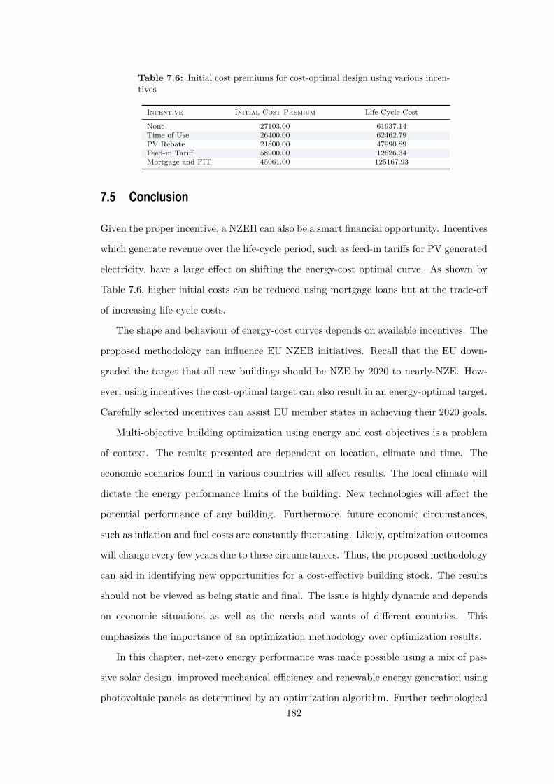
Table 7.6: Initial cost premiums for cost-optimal design using various incen-tives

Incentive Initial Cost Premium Life-Cycle Cost

None 27103.00 61937.14Time of Use 26400.00 62462.79PV Rebate 21800.00 47990.89Feed-in Tariff 58900.00 12626.34Mortgage and FIT 45061.00 125167.93

7.5 Conclusion

Given the proper incentive, a NZEH can also be a smart financial opportunity. Incentives

which generate revenue over the life-cycle period, such as feed-in tariffs for PV generated

electricity, have a large effect on shifting the energy-cost optimal curve. As shown by

Table 7.6, higher initial costs can be reduced using mortgage loans but at the trade-off

of increasing life-cycle costs.

The shape and behaviour of energy-cost curves depends on available incentives. The

proposed methodology can influence EU NZEB initiatives. Recall that the EU down-

graded the target that all new buildings should be NZE by 2020 to nearly-NZE. How-

ever, using incentives the cost-optimal target can also result in an energy-optimal target.

Carefully selected incentives can assist EU member states in achieving their 2020 goals.

Multi-objective building optimization using energy and cost objectives is a problem

of context. The results presented are dependent on location, climate and time. The

economic scenarios found in various countries will affect results. The local climate will

dictate the energy performance limits of the building. New technologies will affect the

potential performance of any building. Furthermore, future economic circumstances,

such as inflation and fuel costs are constantly fluctuating. Likely, optimization outcomes

will change every few years due to these circumstances. Thus, the proposed methodology

can aid in identifying new opportunities for a cost-effective building stock. The results

should not be viewed as being static and final. The issue is highly dynamic and depends

on economic situations as well as the needs and wants of different countries. This

emphasizes the importance of an optimization methodology over optimization results.

In this chapter, net-zero energy performance was made possible using a mix of pas-

sive solar design, improved mechanical efficiency and renewable energy generation using

photovoltaic panels as determined by an optimization algorithm. Further technological182

advances will undoubtedly improve thermal storage, reduce peak loads, improve controls

and enable distributed grids. However, without further economies of scale or strong eco-

nomic incentives, net-zero energy buildings will likely remain a small fraction of the

building stock due to their additional upfront costs.

Further research is needed to identify incentives which reduce initial and life-cycle

costs by generating revenue over the life-cycle period. These types of incentives greatly

improve the life-cycle cost outcome. Further work should focus on collaborating with

policy makers to ensure that future buildings are both cost and energy optimal.

183

Chapter 8

Effect of a Time-of-Use Feed-In Tariff on

Optimal Net-Zero Energy Home Design

“In some ways I think that scientists have misled themselves into thinking thatif you collect enormous amounts of data you are bound to get the right answer.You are not bound to get the right answer unless you are enormously smart. Youcan narrow down your questions; but enormous data sets often consist of enormousnumbers of small sets of data, none of which by themselves are enough to solve thething you are interested in, and they fit together in some complicated way.

–Bradley Efron ”8.1 Overview

This chapter builds on successful incentives proposed in the previous chapter, in

particular, the effect of a feed-in tariff on optimal NZEH design. As recommended

in the previous chapter, technology costs are amortized in life-cycle cash flows. This

assumes that roof-installed PV panels are considered by mortgage lenders as part of the

property value. A time-of-use FIT is explored to investigate cash-flow improvements

and how such an incentive affects optimal buildings design. This section demonstrates

the utility of conservation and efficiency measures to reduce the net-payback of a NZEH.

However, projected future PV panel costs suggest that this relationship may change in

the coming decade. To achieve this, archetype solar home proposed in chapter 4 is used

in the case-study. The optimization methodology and approach proposed is important

in identifying future interactions using yet unknown economics. In this chapter, large

sets of interacting optimization data are reduced to simple economic metrics, in order to184

better understand the relationship between energy conservation measures and renewable

energy generation in optimal building design.

8.2 Background

In the last 10 years, the PV industry has undergone a significant transformation. PV

panel prices have dropped much more quickly than anticipated. The IEA PVPS (2013)

anticipated that global price of PV would approach $1/W by 2017. Globally, a PV

panel is manufactured at $1.15/W in 2012 and is predicted to decrease to $0.85/W by

2014 (IEA PVPS, 2013). Furthermore, the cost of manufacturing PV panels is decreasing

by 20% per year (Breyer and Gerlach, 2010) with conversion efficiencies approaching

25%. At the beginning of this PhD (2009), market-ready PV was sold at almost $4/W

(not installed) and was only 14% efficient! The DOE SunShot initiative aims to provide

opportunities to facilitate innovation in the market and reduce installed PV panel costs

at 25% efficiency to $0.5/W and total installed costs (including panel price) to $1/W by

2020 (DOE, 2013). The SunShot initiative is offering a ten million dollar prize to the

first company who achieves this task. At the $1/W installed price point, it is believed

that PV can compete directly with all other forms of electricity generation in the US

even with subsidies to fossil fuels. The PV industry is now projected to achieve this goal

by 2020. The idea that solar energy will be cheaper than fossil fuels is not surprising.

Fossil fuels require exploration, environmental review, processing, transportation and

management and without carbon capture and containment scrubbing they negatively

impact the environment. Solar energy originates from an efficient nuclear fusion process

which is abundant, free to use and a virtually inexhaustible form of renewable energy.

However, it is not possible yet to achieve net-zero energy using renewable energy alone.

Rapidly falling PV prices complicates the relationship between improved energy con-

servation approaches to building design, improved mechanical efficiency and renewable

energy generation in optimal building design. For example, at what PV price point is it

more economical to invest in generation over more insulation? From a different perspec-

tive, is it possible that investment gains from cheap, efficient PV might be reinvested

into further efficiency measures to reduce net-energy consumption? Methodologies, not

185

rules-of-thumb are necessary to navigate such complex and constantly fluctuating inter-

actions.

This chapter explores the effect of a TOU FIT incentive and falling PV prices on

optimal building design. The capital payback of a NZEH case-study previously shown

in Chapter 5 is further expanded upon. The relationship between energy conservation

measures and PV generation at different price points is explored using this model.

8.3 Method

A Feed-in-Tariff was developed to create positive cash-flow for PV integrated into the

envelope of a NZEH. Feed-in tariffs for renewable energy generation have been available

since 2009 in Ontario (OPA, 2013). Peak electricity consumption in some large Cana-

dian cities, such as Toronto, is directly correlated with summer cooling (Toronto Hydro,

2011). Cooling loads are caused by peak solar radiation which could be offset using

PV generated electricity. To create a disincentive for electricity use during peak peri-

ods, some provinces in Canada have implemented time-of-use electricity charges. Since

electricity is sold at a higher rate during peak periods, logically, so too should it be pur-

chased at a cost premium. The largest incentive is provided when electricity is needed

the most. Such incentives may cause sub-optimal orientation to improve PV generated

revenue and better reduce peak-grid loads. Utilities benefit since they do not require

expansion of centralized generation to meet peak electricity demands and PV system

owners generate additional revenue during the equipment’s expected lifetime. This in-

centive structure improves a criticism of the present FIT program that tax-payers pay

cost premiums for PV generated electricity when electricity is not at peak demand.

Table 8.1: Time of use Feed-in Tariff

FIT Schedule Hours Peak Incentive, ¢/kWh

Summer Weekdays 21:00–07:00 off-peak 36.607:00–11:00 mid-peak 54.911:00–17:00 on-peak 72.217:00–21:00 mid-peak 54.9

Winter Weekdays 21:00–07:00 off-peak 36.607:00–11:00 on-peak 72.211:00–17:00 mid-peak 54.917:00–21:00 on-peak 72.2

Weekends and Holidays 00:00–24:00 off-peak 36.6

186

Table 8.1 shows the implemented time-of-use feed-in tariff over a 20 year period. Note

that peak electricity mid-purchase rates are based on the microFIT program offering of

54.9¢/kWh in Ontario (OPA, 2013). The off-peak rate was determined by a reduction

multiplier of 1.5. The on-peak rate was set as 2.5 times the off-peak rate.

Using this incentive, along with the energy model proposed in Chapter 3 and the

multi-objective optimization methodology proposed in Chapter 7 a near cost-optimal

design on the Pareto front was identified. Note that economic metrics such as payback

are compared to a reference building as defined in Appendix C.

The next section presents results and a discussion.


A TOU FIT was found to increase annual cash-flows by 20% (approximately $1000) with

a 3% increase in net-energy consumption. The optimal design found in this analysis is

shown in Table 8.2.

Table 8.2: Optimization Results for ÉcoTerra Complete Redesign

Variable Description Units Optimal Values

azi Building orientation/azimuth degrees 12 (SSE)aspect Aspect ratio (south facing width to depth ratio) – 1.4wall_ins Effective resistance of wall insulation m2K/W 8.56ceil_ins Effective resistance of ceiling insulation m2K/W 10.57base_ins Effective resistance of basement wall insulation m2K/W 5.08slab_ins Effective resistance of slab insulation m2K/W 1.39ovr_south Width of Southern Window Overhangs m 0.34pv_area Percent of PV area on roof % 90pv_area_e Percent of PV on east facade % 0pv_area_w Percent of PV on west facade % 0pv_eff PV efficiency % 15roof_slope South facing roof/PV slope degrees 45wwr_s Percent of window to wall ratio, south % 48wwr_n Percent of window to wall ratio, north % 10wwr_e Percent of window to wall ratio, east % 10wwr_w Percent of window to wall ratio, west % 10GT_s Glazing type, south (also N,E,W) – 2heating_sp Heating setpoint ◦C 18cooling_sp Cooling setpoint ◦C 28FT Window Framing Types (1:Wood, 2:Vinyl) – 2slab_th Concrete slab thickness m 0.25vwall_th Concrete wall thickness (basement) m 0.15zone_mix Air circulation rate between thermal zones L/s 133infil Envelope air-tightness (natural infiltration rate) ACH 0.025

f(x) Net-Energy Consumption of Individual kW h -3150g(x) Net-Present Value of Individual $ 32,000

Interestingly, the TOU FIT caused very few design changes compared to previous

chapters. The largest change is the sub-optimal orientation 12 degrees east of south.187

Further inspection found that the algorithm was increasing cash-flow by generating

more electricity during peak periods while slightly reducing the energy performance of

the home. Here, 12 degrees east of south was identified as the optimal trade-off in lost

performance to improve payback. The design strategies found in previous chapters were

equally applicable under the context of sub-optimal orientations.

Figure 8.1 shows the breakdown of cash flow for the FIT incentive and amortization

of initial costs.

−30000−20000−10000

0

0 1 2 3 4 5 6 7 8 9 10 11 12 13 14 15 16 17 18 19 20 21 22 23 24 25 26 27 28 29

Initial/Mortgage Cash Flow

time, yr

Cas

h Fl


positive

negative

−100000

1000020000

0 1 2 3 4 5 6 7 8 9 10 11 12 13 14 15 16 17 18 19 20 21 22 23 24 25 26 27 28 29

Replacement/Maintenance Cash Flow

time, yr

Cas

h Fl


positive

negative

−1000−800−600−400−200

0

0 1 2 3 4 5 6 7 8 9 10 11 12 13 14 15 16 17 18 19 20 21 22 23 24 25 26 27 28 29

Utility Cost Cash Flow

time, yr

Cas

h Fl


positive

negative

0100020003000400050006000

0 1 2 3 4 5 6 7 8 9 10 11 12 13 14 15 16 17 18 19 20 21 22 23 24 25 26 27 28 29

PV Revenue Cash Flow

time, yr

Cas

h Fl


positive

negative

−20000−10000

0

0 1 2 3 4 5 6 7 8 9 10 11 12 13 14 15 16 17 18 19 20 21 22 23 24 25 26 27 28 29

Total Cash Flow

time, yr

Cas

h Fl


positive

negative

Figure 8.1: Cash flow diagram of optimal design using FIT incentive and mortgage

Figure 8.2 shows total cash flow for the optimal design compared to the total cash

flow of the reference design. The cumulative sum shows the optimal NZEH has a capital

payback of 9 years. The internal rate of return for this cash flow difference is 5%.

188

−20000

−10000

0

0 1 2 3 4 5 6 7 8 9 10 11 12 13 14 15 16 17 18 19 20 21 22 23 24 25 26 27 28 29


time, yr

Cas

h Fl


positive

negative

−10000

−5000

0

0 1 2 3 4 5 6 7 8 9 10 11 12 13 14 15 16 17 18 19 20 21 22 23 24 25 26 27 28 29


time, yr

Cas

h Fl


positive

negative

−15000

−10000

−5000

0

5000

0 1 2 3 4 5 6 7 8 9 10 11 12 13 14 15 16 17 18 19 20 21 22 23 24 25 26 27 28 29


time, yr

Cas

h Fl


positive

negative

−15000−10000−5000

05000

0 1 2 3 4 5 6 7 8 9 10 11 12 13 14 15 16 17 18 19 20 21 22 23 24 25 26 27 28 29


time, yrCum

ulat

ive

Cas

h Fl

ow, $


negative

Figure 8.2: Cash flow diagram: Optimal design compared to reference building

Table 8.3 shows the capital payback of various conservation measures relative to the

reference home.

Table 8.3: Sample of capital payback of design upgrades from reference to optimal design

Variable Description Reference Optimal Units Payback, yr

pv_area Percent of PV area on roof 0 90 % 10.5

GT_s Glazing type, south dbl-glaze dbl-glazeEStar

– 2.5

ceil_ins Effective resistance of ceiling insula-tion

8.8 10.57 m2K/W 10

wwr_s Percent of window to wall ratio, south 25 48 % 3.0wall_ins Effective resistance of wall insulation 4.4 8.56 m2K/W 3.9blind_irr Incident solar radiation for blind de-

ployment0 150 W/m2 3.8

Combined payback from reference to optimal 9.1

Under present economic scenarios, the capital payback of conservation measures are

less than the capital payback of PV panels. Effectively, conservation measures reduced

the net-payback of PV panels relative to the reference building. For example, better

insulation and improving solar access had economic paybacks in the sub five year range

whereas further improving ceiling insulation and adding solar panels had paybacks nearer

to 10 years. Combining both measures under one capital investment had a net-payback189

of 9.1 years.

The following figures explore scenarios for increasing utility costs and reduced PV

panel costs. Figure 8.3 shows total cash flow for the optimal design compared to the

total cash flow of the reference design with electricity prices at 14¢/kWh. Under the

scenario of electricity prices at 14¢/kWh, payback is achieved after 6.5 years.

−30000

−20000

−10000

0

0 1 2 3 4 5 6 7 8 9 10 11 12 13 14 15 16 17 18 19 20 21 22 23 24 25 26 27 28 29


time, yr

Cas

h Fl


positive

negative

−15000

−10000

−5000

0

0 1 2 3 4 5 6 7 8 9 10 11 12 13 14 15 16 17 18 19 20 21 22 23 24 25 26 27 28 29


time, yr

Cas

h Fl


positive

negative

−10000−5000

05000

0 1 2 3 4 5 6 7 8 9 10 11 12 13 14 15 16 17 18 19 20 21 22 23 24 25 26 27 28 29


time, yr

Cas

h Fl


positive

negative

−10000

0

10000

20000

0 1 2 3 4 5 6 7 8 9 10 11 12 13 14 15 16 17 18 19 20 21 22 23 24 25 26 27 28 29


time, yrCum

ulat

ive

Cas

h Fl

ow, $


negative

Figure 8.3: Cash flow diagram: Optimal design compared to reference building. Utility pricesat 14¢/kWh.

Figure 8.4 shows total cash flow for the optimal design compared to the total cash

flow of the reference design with PV panel prices at 1.0$/W or 2.5$/W installed and

electricity prices at 14¢/kWh. Under the scenario of electricity prices at 14¢/kWh and

PV panel installed costs of $2.5, capital payback of 3 years is achieved.

190

−20000

−10000

0

0 1 2 3 4 5 6 7 8 9 10 11 12 13 14 15 16 17 18 19 20 21 22 23 24 25 26 27 28 29time, yr

Cas

h Fl


positive

negative


−15000

−10000

−5000

0

0 1 2 3 4 5 6 7 8 9 10 11 12 13 14 15 16 17 18 19 20 21 22 23 24 25 26 27 28 29time, yr

Cas

h Fl


positive

negative


−5000

0

0 1 2 3 4 5 6 7 8 9 10 11 12 13 14 15 16 17 18 19 20 21 22 23 24 25 26 27 28 29time, yr

Cas

h Fl


positive

negative


−100000

100002000030000

0 1 2 3 4 5 6 7 8 9 10 11 12 13 14 15 16 17 18 19 20 21 22 23 24 25 26 27 28 29time, yrC

umul

ativ

e C

ash

Flow

, $


negative


Figure 8.4: Cash flow diagram: Optimal design compared to reference building. PV prices at1.0$/W and electricity prices at 14¢/kWh.

8.5 Conclusion

With targeted incentives, NZEH can have an payback that is more attractive and stable

than other market options. Typically, consumers and business will act on investments

with capital paybacks in the 5–7 year range. Given the projected future cost of PV, the

net-payback of such technology could be less than five years in the coming decade.

Using a TOU FIT incentive, the algorithm found that it was more cost-effective to

orientate the primary solar collector twelve degrees east of south rather than orientating

directly south and using solar panels on the east or west facades. This design choice

had two benefits: (1) more energy was generated during peak times which increases

annual income, and (2) the slightly east-oriented passive solar glazing surface was able

to reduce the heating-system dependency when transitioning from a nightly set-back

schedule to the morning heating schedule. This reduced heating system peak-loads

without significantly changing annual heating consumption. West-facing glazing surfaces

were not selected since they typically resulted in overheating of living spaces.

The relationship between economic payback from energy conservation and efficiency

191

measures with electricity generation is changing quickly. Presently, energy conservation

measures reduce the burdensome investment of more expensive renewable energy invest-

ments in PV panels. Given the rapid reduction of PV panel price, this relationship may

inverse in the near future, where energy generation technology aids in the payback of en-

ergy conservation measures. Methodologies that are those useful which aid designers in

understanding the energy and cost paybacks in building design under quickly changing

markets.

192

Chapter 9

Conclusion

“Automate the mundane—liberate the creative.–Drew Crawley (on the future of building energy modelling)”

9.1 Summary

This thesis explored the following research areas: (i) performance enhancements to

optimization algorithms applied to building research; (ii) use of optimization algo-

rithms in uncertainty analysis around performance criterion; (iii) potential for economic

incentives to affect energy-cost optimal curves; and (iv) effect of economic incentives on

optimal NZEH design.

This thesis was structured as follows. Chapter 3 provided the design concepts used

in this thesis. Chapter 4 showed a multi-objective design of an archetype solar home

using the optimization algorithm, cost and energy model presented in Chapter 3. The

archetype NZEH which combined passive solar design, energy efficiency measures in-

cluding a geothermal heat pump and building-integrated photovoltaics was used in later

chapters. Chapter 5 elaborated on how information obtained from previous simulations

can be used to improve search convergence properties and optimization results using

deterministic searches coupled with an evolutionary algorithm. The improvements in

convergence speed and accuracy allowed for repeated optimization runs to build statis-

tical significance in later chapters. Chapter 6 introduced a methodology to estimate the

influence of building design parameter variations on the performance an energy model.

This analysis improved the robustness of a design in meeting the NZE criterion by vi-193

sualizing which design variations most significantly affect the archetype NZEH design.

Chapter 7 describes an optimization methodology to establish and compare potential

policies which incentivize cost optimal net-zero energy buildings. Using the incentive

structures proposed in Chapter 7, Chapter 8 explores the effect of a time-of-use feed-in

tariff and reductions in PV panel costs on optimal NZEH design.

Optimization methodologies in building simulation is an important research area.

The reality is that no single optimization result can be generalized for all potential de-

sign scenarios. For example, custom home-builders have different framing billing-rates

and time-requirements than pre-fabrication builders. Also, the energy costs and weather

conditions are specific to the building location. Furthermore, the cost of photovoltaic

panels is dropping quickly and becoming cost-competitive with energy efficiency mea-

sures. Thus, this thesis focused on methodologies to generate results quickly for any

location with emphasis on facilitating the identification of optimal design opportunities

that combine energy efficiency measures with building integrated solar systems such as

passive solar systems and building integrated photovoltaics.

The proposed algorithm performance enhancements reduced the time requirements

from 40–50 hours, see chapter 2, to less than two hours on a personal laptop. This

made it possible to explore repetitive optimization analysis and to extract statistical

information from the solution space into a database. The information stored in the

database made it possible to extract PDFs for use in a variability analysis. The vari-

ability analysis identified potential changes which significantly effect the net-zero energy

performance criterion. Finally, the effect of economic incentives on energy-cost optimal

curves was explored. It was identified that under certain incentive structures, a cost-

optimized building could be synonymous with a performance-optimized building with

capital paybacks approaching 5 years.

In achieving these research goals, several unexpected tools were identified. PDFs

enabled the visualization of design trade-offs around the NZE performance objective.

Using PDFs, design variable limits were identified for several influential variables such

as energy-related occupant behaviour, solar orientation of the building, wall insulation

levels and window-to-wall ratios. Back-tracking searches identified steepest gradient

pathways from reference buildings to performance-optimized buildings. Energy-cost

194

curves were found to be an ideal tools to identify effective incentives. In addition to

these tools, several contributions were made to the field of building engineering.

9.2 Contributions

This thesis proposed a methodology to achieved robust performance-optimized net-zero

energy buildings. The contributions of this thesis are roughly divided into four areas:

1. A methodology for integrating strategic deterministic searches into an evolutionary

algorithm to improve solution quality and algorithm convergence speed for building

optimization problems.

2. A methodology to approximate the uncertainty in building energy consumption

due to cumulative variations in influential variables.

3. A methodology to determine the effect of policies and incentives to aid cost-optimal

NZEHs.

4. Effect of a Time-of-Use Feed-In Tariff on Optimal Net-Zero Energy Home Design.

Several contributions to new performance-optimized simulation approaches are:

1. Development and demonstration of the use of probability density functions ex-

tracted from optimization results to identify performance opportunities and po-

tential design summaries.

2. Development and demonstration of back-tracking searches to identify performance

gradients between one-to-many and one-to-one building comparisons. Importance

factors were introduced to summarize back-tracking results.

Contributions to optimization tool developments are:

1. Development of optimization tool and cost model for building simulation studies.

2. Extraction of variable interactions using mutual information for determining sub-

population searches in an optimization algorithm.

195

3. Algorithm performance improvements specific to the needs of building research

such as adaptive diversity control, preferential deterministic searches, use of gen-

eration gaps to grow multi-objective populations, parallel execution of building

simulations and a differential mutation operator which resulted in factor of 10

time improvement over other tools used in building optimization research with

better resolution of optimum solutions.

9.3 Future Work

There are many opportunities to further develop, refine and apply the scope of research

proposed in this thesis. This section describes potential future work related to: (i) fur-

ther improvements to optimization algorithms; (ii) other application areas of optimiza-

tion research; (iii) implications of different occupant usage and a changing climate on

performance-optimized buildings; (iv) integration of visual and thermal comfort as an

additional objective or constraint; (v) cost model improvements; and (vi) energy model

improvements.

There are still several potential opportunities to further improve algorithm speed

and convergence performance, such as:

1. Applying simplified models to replace time-expensive building simulations using

online training methods from previous simulation data. Several simplified mod-

elling techniques could be explored such as artificial neural networks, decision tree

ensembles, and regression models. Training of simplified models can further reduce

the simulation requirements for building simulation and expedite the optimization

process.

2. Further improvements to the diversity control within the optimization algorithm.

The adaptive control method proposed, which modified selection pressure, can be

greatly improved resulting in better algorithm convergence. For example, using

specialized genetic operators depending on the convergence issue the algorithm is

confronted with.

3. Further exploration on how previous optimization and building simulation data

can be exploited to further improve decision making.196

4. Expedite back-tracking searches by identifying non-full-factorial simulation ap-

proaches to reduce time and computational requirements.

5. Further elaboration on specialized sub-population searches using data extracting

from previous simulations. For example, isolating clusters of interacting variables

within sub-specialized searches. Further explore specialized deterministic searches

for weakly interacting sub-clusters.

There are still many potential application areas for optimization tools and the

methodologies proposed in this thesis within the scope of building research. For ex-

ample:

1. Apply the proposed energy and cost optimization methodologies to commercial and

industrial buildings. Identify incentive opportunities for cost-optimized industrial

and commercial NZEBs.

2. Further validate the proposed methodologies by using the optimization tool de-

veloped for building retrofit. The goal would be to provide guidance on how to

convert the existing residential or commercial building stock to NZE. Decision

analysis would determine if energy measures should be performed now or in the

near future. Analysis includes HVAC systems falling out of calibration and prob-

abilistic projections of future economic scenarios.

3. Apply the optimization tool to larger problems with more than 50 variables such

as a neighbourhood of NZEBs with centralized thermal and electricity storage.

It is likely that different occupant usage patterns and the changing climate will play

a role in determining what a performance-optimized building is. The methodology could

be expanded to identify compromises in design to best suit the uncertain climate change,

occupant usage or economic scenarios. In present research probabilistic approaches are

used to quantify uncertainty in occupant behaviour and climate change. An advantage in

implementing probabilistic approaches is that variations in building usage can be better

reflected in fitness functions used in the optimization analysis. This allows for variability

in objective functions to be quantified and additional simulations are conducted. A

disadvantage in this approach is that fitness evaluations would no longer be deterministic197

which would complicated the extraction of information for strategic search techniques.

Often this design approach is referred to as robust design where buildings are designed

resilient to future unknown or uncertain circumstances. Optimized design could be

viewed as trade-off decision, based on estimates of future scenarios.

The proposed methodology could benefit from the integration of a thermal comfort

model applicable to NZEBs. In the PhD thesis of Carlucci (2012), over 25 thermal

comfort models were evaluated for their suitability of use in a NZEH model. It was

found that only particular thermal comfort approaches best evaluated thermal comfort of

occupants across variations in locations and seasons. Comfort models could be integrated

into the methodology as an objective function or a constraint to better quantify occupant

comfort.

The energy model could be expanded to include better thermal zoning control using

specialized mechanical systems in the house. For example, bedrooms are typically unoc-

cupied outside of sleeping hours. Heating and cooling of these zones could be controlled

based on occupancy. By only heating occupied rooms, heating and cooling loads could

be further reduced. Mechanical equipment such as a variable refrigerant flow system or

radiant floors with control valves could achieve such control.

The house energy model could be expanded to include other market-ready or near

market-ready technologies, such as phase-change materials, masonry wood-stoves and

daily and seasonal thermal storage cisterns. There are economies of scale for community-

based storage systems that cannot realized on a single detached home basis. Many

control strategies could be deployed for system-level and sub-system level control of:

(i) charging of thermal storage; (ii) peak-load reductions via electrical storage or load

shedding; and (iii) control of centralized and localized renewable energy production.

Cost optimization research could be expanded to determine feasible price points for new

building materials such as aerogel insulation or electrochromic windows. The integration

of occupant comfort models into the energy model could be further explored.

There is opportunity to include advanced control strategies into net-zero energy

building design. Such strategies might include: (i) model predicative control, (ii) mod-

ular conditioning of zones depending on occupancy, and (iii) model interactions with

grid-signals to shed peak loads. For example, if excess renewable electricity was be-

198

ing generated in the grid, utilities could ask residential consumers to charge electric

hot-water tanks to reduce later peak-electricity consumption.

9.4 Final Thoughts

“To imagine is to perceive many potential futures, select the most delightfulpossibility, and then pull the present forward to meet it.

–Imaginary Foundation ”This thesis demonstrated a methodology to achieve performance-optimized net-zero

energy buildings. Optimization approaches explored and found optimal trade-offs be-

tween energy and cost optimized buildings. A variability analysis aided in better un-

derstanding the robustness of the NZEH design. In the last two chapters, previously

developed tools were used to explore how incentives change the approach of optimal

building design.

Optimization tools enhance our decision making capabilities. With these approaches,

we can navigate complicated trade-offs in economics and performance, and can identify

scenarios where uncertainty in unknown variables is significant. We can look at all

possible paths, identify opportunities to best achieve our building performance objec-

tives and make these opportunities a reality. By automating mundane simulation tasks,

optimization tools enhance our decision making abilities by focusing our attention on

significant design opportunities and away from repetitive energy simulation. Many ben-

efits are achieved for this effort including: better occupant comfort, improved indoor

air-quality, possible investment opportunities, and resilient investments to mitigate cli-

mate change and energy cost escalation. By identifying opportunities for performance-

optimized buildings, optimization approaches enhance our imagination making us aware

of achievable performance targets.

Recall the polarizing view regarding the application of optimization algorithms pre-

sented at the end of the introduction. One view is that only artificially-intelligent algo-

rithms will design performance-optimized buildings of the future. No amount of human

innovation can identify scenarios which both meet performance objectives while sat-

isfying occupant comfort. On the opposing side is the view that algorithms cannot

understand the cultural or social implications of a particular design, thus they result199

in unusable information. It is possible that algorithms will never completely design a

building. There are many cultural and æsthetics implications that an algorithm cannot

yet, and may never, embody. However, there are areas that algorithms excel at. Herein

lies their true potential. Optimization approaches are tools. Tools which sculpt po-

tential solutions to unsolved and ill-defined problems. Optimization tools can propose

unprecedented solutions to tough problems. Perhaps their potential has yet to be fully

realized since the toughest problems are yet to come.

200

References

Abley, M., 1998. The Ice Storm: An Historic Record In Photographs of January 1998,1st Edition. McClelland and Stewart.

Al-Homoud, M. S., 2005. A systematic approach for the thermal design optimization ofbuilding envelopes. Journal of Building Physics 29 (2), 95–119.

Amdahl, G., 1967. Validity of the single processor approach to achieving large-scalecomputing capabilities. In: Proceedings of AFIPS. New York, US, pp. 483–485.

Anderson, R., Christensen, C., Horowitz, S., 2006. Analysis of residential system strate-gies targeting least-cost solutions leading to net zero energy homes. ASHRAE Trans-actions 112 (2), 330–341.

Andre, D., Koza, J.R., 1998. A parallel implementation of genetic programming thatachieves super-linear performance. Information Sciences 106 (3-4), 201.

Armstrong, M. M., Swinton, M. C., Ribberink, H., Beausoleil-Morrison, I., Millette, J.,2009. Synthetically derived profiles for representing occupant–driven electric loads inCanadian housing. Journal of Building Performance Simulation 2 (1), 15–30.

Arndt, D., Baringer, M., Johnson, M., 2010. Published on July 28, 2010 by the NationalOceanic and Atmospheric Administration.URL http://www.ncdc.noaa.gov/bams-state-of-the-climate/

ASHRAE, 2002. ASHRAE guideline 14: Measurement of energy and demand savings.Retrieved February 2013.URL https://www.ashrae.org/standards-research--technology/standards--guidelines/titles-purposes-and-scopes#Gdl14

ASHRAE, 2011a. ASHRAE standard 62.2.URL http://www.ashrae.org/standards-research--technology/standards--guidelines

ASHRAE, 2011b. ASHRAE standard 90.1.URL http://www.ashrae.org/standards-research--technology/standards--guidelines

201

ASHRAE, 2011c. HVAC Applications. American Society of Heating, Refrigerating andAir-Conditioning, Atlanta, USA.

Athena, 2011. Athena impact estimator for buildings. Retrieved May 2011.URL http://www.athenasmi.org/our-software-data/impact-estimator/

Athienitis, A., Santamouris, M., 2002. Thermal Analysis and Design of Passive SolarBuildings. James & James, London, UK.

Attia, S., Hamdy, M., OâĂŹBrien, W., Carlucci, S., 2013. Assessing gaps and needsfor integrating building performance optimization tools in net zero energy buildingsdesign. Energy and Buildings 60 (0), 110–124.

Aude, P., Tabary, L., Depecker, P., 2000. Sensitivity analysis and validation of buildings’thermal models using adjoint-code method. Energy and Buildings 31 (3), 267–283.

Audet, C., Dennis, J.E., 2002. Analysis of generalised pattern searches. SIAM Journalof Optimization 13 (3), 889–903.

Augenbroe, G., de Wilde, P., Moon, H. J., Malkawi, A., 2004. An interoperability work-bench for design analysis integration. Energy and Buildings 36 (8), 737–748.

Balachandran, M., Gero, J. S., 1987. Dimensioning of architectural floor plans underconflicting objectives. Environment and Planning B 14, 29–37.

Balcomb, J. D., 1992. Passive Solar Buildings, 1st Edition. The MIT Press, Cambridge,USA.

Bank of Canada, 2009. Rates and Statistics: Interest rates, Canadian interest rates.Accessed January, 2013.URL http://www.bankofcanada.ca/rates/interest-rates/

Beausoleil-Morrison, I., 1996. BASECALC: A software tool for modelling residentialfoundation heat losses. In: Proceedings of the Third Canadian Conference in Com-puting in Building and Civil Engineering.

Beausoleil-Morrison, I., 2000. The adaptive coupling of heat and air flow modeling withindynamic whole-building simulations. Ph.D. dissertation, University of Strathclyde.

Beausoleil-Morrison, I., Griffith, B., Vesanen, T., Weber, A., 2009. A demonstrationof the effectiveness of inter-program comparative testing for diagnosing and repair-ing solution and coding errors in building simulation programs. Journal of BuildingPerformance Simulation 2 (1), 63–73.

Beausoleil-Morrison, I., Macdonald, F., Kummert, M., McDowell, T., Jost, R., 2013.Co-simulation between esp-r and trnsys. Journal of Building Performance Simulation0 (0), 1–19.

Beausoleil-Morrison, I., Macdonald, F., Kummert, M., McDowell, T., Jost, R., Fergu-son, A., 2011. The design of an esp-r and trnsys co-simulator. In: Proc. BuildingSimulation. pp. 2333–2340.

Beccali, G., Cellura, M., Brano, V. L., Orioli, A., 2005. Is the transfer function methodreliable in a european building context? a theoretical analysis and a case study in thesouth of italy. Applied Thermal Engineering 25 (2-3), 341–357.

202

Berggren, B., Hall, M., Wall, M., 2013. LCE analysis of buildings - Taking the steptowards Net Zero Energy Buildings. Energy and Buildings 62 (0), 381–391.

Bledsoe, W. W., Browning, I., December 1959. Pattern recognition and reading bymachine. pp. 225–232, the 1959 Eastern Joint Computer Conference for The NationalJoint Computer Committee.

Booth, A., Choudhary, R., 2013. Decision making under uncertainty in the retrofit anal-ysis of the UK housing stock: Implications for the green deal. Energy and Buildings64 (0), 292–308.

Borchiellini, R., Fürbringer, J.-M., 1999. An evaluation exercise of a multizone air flowmodel. Energy and Buildings 30 (1), 35–51.

BPIE, 2010. Cost optimality: Discussing methodology and challenges within the recastEnergy Performance of Buildings Directive.URL http://www.bpie.eu/cost_optimality.html

Breesch, H., Janssens, A., 2010. Performance evaluation of passive cooling in officebuildings based on uncertainty and sensitivity analysis. Solar Energy 84 (8), 1453–1467.

Breyer, C., Gerlach, A., 2010. Global overview on grid-parity event dynamics. In: Pro-ceedings of 25th EU PVSEC/WPEC-5. Valencia, ES, pp. 6–10.

Brohus, H., Frier, C., Heiselberg, P., Haghighat, F., 2012. Quantification of uncertaintyin predicting building energy consumption: A stochastic approach. Energy and Build-ings 55 (0), 127–140.

Bucking, S., Athienitis, A., Zmeureanu, R., 2011. Optimization of net-zero energy solarcommunities: effect of uncertainty due to occupant factors. In: Proceedings of ISESWorld Conference, Kassel, Germany.

Bucking, S., Athienitis, A., Zmeureanu, R., 2013a. Multi-objective optimal design ofa near net-zero energy solar house. ASHRAE Transactions 0 (0), 1–26, accepted forpresentation.

Bucking, S., Athienitis, A., Zmeureanu, R., O’Brien, W., Doiron, M., 2010. Design opti-mization methodology for a near net zero energy demonstration home. In: Proceedingsof EuroSun International Conference on Solar Heating, Cooling and Buildings. Euro-Sun, Graz, Austria.

Bucking, S., Zmeureanu, R., Athienitis, A., 2013b. An information driven hybrid evolu-tionary algorithm for optimal design of a net zero energy house. Solar Energy 96 (0),128–139.

Bucking, S., Zmeureanu, R., Athienitis, A., 2013c. A methodology for identifying theinfluence of design variations on building energy performance. Journal of BuildingPerformance Simulation, 1–26.

Bucking, S., Zmeureanu, R., Athienitis, A., 2013d. An optimization methodology toevaluate the effect size of incentives on energy-cost optimal curves. In: Proceedings ofThirteenth International IBPSA Conference, Chambéry, France. pp. 1–8.

203

Buhl, W.F., Erdem, F.C., Winkelmann, F.C., Sowell, E.F., 1993. Recent improvementsin SPARK: Strong component decomposition, multivalued objects, and graphical in-terface. In: Proceedings of Building Simulation, Adelaide, Australia. IBPSA.

Burhenne, S., Jacob, D., Henze, G., 2010. Uncertainty analysis in building simulationwith monte carlo techniques. In: Proceedings of SimBuild, 3rd National Conferenceof IBPSA-USA New York, USA. International Building Performance Simulation As-sociation, USA chapter.

Burhenne, S., Tsvetkova, O., Jacob, D., Henze, G. P., Wagner, A., 2013. Uncertaintyquantification for combined building performance and cost-benefit analyses. Buildingand Environment 62 (0), 143–154.

Caldas, L., September 2001. An evolution-based generative design system: Using adap-tion to shape architectural form. Ph.D. dissertation, Massachusetts Institute Technol-ogy.

Caldas, L., 2008. Generation of energy-efficient architecture solutions applyingGENE_ARCH: An evolution-based generative design system. Advanced EngineeringInformatics 22 (1), 59–70.

Candanedo, J., 2011. A Study of Predictive Control Strategies for Optimally DesignedSolar Homes. Ph.D. dissertation, Concordia University.

Candanedo, L., Athienitis, A., Candanedo, J., O’Brien, W., Chen, Y., 2010. Tran-sient and Steady State Models for Open-Loop Air-Based BIPV/T Systems. ASHRAETransactions 116 (1), 600–620.

Carlucci, S., March 2012. An automated optimization process to support the design ofcomfortable net zero energy buildings. Ph.D. dissertation, Dipartimento Di Scienza eTecnologie Dell’Ambiente Costruito.

Castro-Lacouture, D., Sefair, J. A., Flórez, L., Medaglia, A. L., 2009. Optimizationmodel for the selection of materials using a leed-based green building rating systemin colombia. Building and Environment 44 (6), 1162–1170.

Chakraborty, U., 2008. Advances in Differential Evolution, 1st Edition. Springer-Verlag,Heidelberg, DE.

Charron, R., 2007. Development of a genetic algorithm optimisation tool for the earlystage design of low and net-zero energy solar homes. Ph.D. dissertation, ConcordiaUniversity.

Chen, Y., 2009. Modeling and design of a solar house with focus on a ventilated con-crete slab with a building-integrated photovoltaic/thermal system. Master’s thesis,Concordia University.

Chen, Y., Athienitis, A., Galal, K., 2010a. Modeling, design and thermal performance ofa BIPV/T system thermally coupled with a ventilated concrete slab in a low energysolar house: Part 1, BIPV/T system and house energy concept. Solar Energy 84 (11),1892–1907.

Chen, Y., Galal, K., Athienitis, A., 2010b. Modeling, design and thermal performanceof a BIPV/T system thermally coupled with a ventilated concrete slab in a low energysolar house: Part 2, ventilated concrete slab. Solar Energy 84 (11), 1908 – 1919.

204

Chiras, D. D., 2002. The Solar House: Passive Heating and Cooling, 1st Edition. ChelseaGreen, White River, VT .

Choudhary, R., Spring 2004. A hierarchical optimization framework for simulation-basedarchitectural design. Ph.D. dissertation, University of Michigan.

Choudhary, R., Malkawi, A., Papalambros, P., 2003. A hierarchical design optimizationframework for building performance analysis. In: Building Simulation. IBPSA, pp.179–999.

Choudhary, R., Malkawi, A., Papalambros, P., 2005. Analytic target cascading insimulation-based building design. Automation in Construction 14, 551–568.

Chow, T. J., Hand, J., Strachan, P., 2003. Building-integrated photovoltaic and thermalapplications in a subtropical hotel building. Applied thermal engineering 23 (16),2035–2049.

Christensen, C., Barker, G., Horowitz, S., 2004. A sequential search technique for iden-tifying optimal building designs on the path to zero net energy. In: Proceedings of theSolar 2004. American Solar Energy Society.

Clarke, J., 2001. Energy Simulation In Building Design, 2nd Edition. Butterworth-Heinemann, Oxford, UK.

CMHC, 2008. Canada Mortgage and Housing Corporation EQuilbrium Homepage. Re-trieved July, 2013.URL http://www.cmhc-schl.gc.ca/en/co/maho/yohoyohe/heho/eqho/index.cfm

CMHC, 2012. Accessed November, 2012.URL http://www.cmhc-schl.gc.ca/en/corp/faq/faq_006.cfm

Coello Coello, C., 1999. An updated survey of evolutionary multiobjective optimizationtechniques: State of the art and future trends. In: Proceedings of the 1999 Congresson Evolutionary Computation. IEEE Press, Piscataway, NJ.

Coello Coello, C., 2002. Theoretical and numerical constraint-handling techniques usedwith evolutionary algorithms: a survey of the state of the art. Computer Methods inApplied Mechanics and Engineering 191 (11), 1245.

Coley, D. A., Schukat, S., 2002. Low-energy design: combining computer-based optimi-sation and human judgement. Building and Environment 37 (12), 1241–1247.

Corrado, V., Mechri, H., 2009. Uncertainty and sensitivity analysis for building energyrating. Journal of Building Physics 44 (6), 1538–1544.

Couchoulas, O., Spring 2003. Shape evolution: an algorithmic method for conceptualarchitectural design combining shape grammars and genetic algorithms. Ph.D. disser-tation, University of Bath.

Cover, T., Tomas, J., 2006. Elements of Information Theory, 2nd Edition. Wiley, Hobo-ken, NJ.

Crawley, D., Huang, J., 1997. Does It Matter Which Weather Data You Use in EnergySimulations? Accessed Nov 2011.URL http://simulationresearch.lbl.gov/dirpubs/1801_weath.pdf

205

Crawley, D.B., Hand, J.W., Kummert, M., Griffith, B.T., 2008. Contrasting the capabil-ities of building energy performance simulation programs. Building and Environment43 (4), 661–673.

Crawley, D. B., Pedersen, C. O., Lawrie, L. K., Winkelman, F. C., 2000. Energyplus:Energy simulation program. ASHRAE Journal 42, 49–56.

Davis, L., 1987. Genetic algorithms and simulated annealing. Morgan Kaufman Pub-lishers, Los Altos, USA.

Day4Energy, 2012. Day4Energy model 48MC Premium Photovoltaic Modules. RetrievedNov 2012.URL http://simulationresearch.lbl.gov/dirpubs/1801_weath.pdf

D’Cruze, N.A., Radford, A.D., 1987. A multicriteria model for building performanceand design. Building and Environment 3 (22), 167–179.

D’Cruze, N.A., Radford, A.D., Gero, J.S., 1983. A pareto optimization problem formu-lation for building performance and design. Engineering Optimization 7, 17–33.

Deb, K., 2001. Multi-objective optimization using evolutionary algorithms, 1st Edition.Wiley, New York, USA.

Deb, K., Pratap, A., Agarwal, S., Meyarivan, T., 2002. A fast and elitist multiobjectivegenetic algorithm: NSGA-II. IEEE Transactions on Evolutionary Computation 6,182–197.

Déqué, F., Ollivier, F., Poblador, A., 2000. Grey boxes used to represent buildings witha minimum number of geometric and thermal parameters. Energy and Buildings 31,29 – 35.

De Wit, S., 2001. Uncertainty in predictions of thermal comfort in buildings. Ph.D.dissertation, Delft University.

De Wit, S., Augenbroe, G., 2002. Analysis of uncertainty in building design evaluationsand its implications. Energy and Buildings 34 (9), 951–958.

De Wit, S., Augenbroe, G., 2004. Analysis of uncertainty in building design evaluationsand its implications. Energy and Buildings 34, 951.

Diakaki, C., Grigoroudis, E., Kabelis, N., Kolokotsa, D., Kalaitzakis, K., Stavrakakis,G., 2010. A multi-objective decision model for the improvement of energy efficiencyin buildings. Energy 35 (12), 5483–5496.

DOE, 2005. DOE Building America Benchmark Model. U.S. Department of Energy.URL http://www.eere.energy.gov/buildings/building_america/docs/benchmark_2005.doc

DOE, 2007. Building Energy Software Tools Directory. Retrieved May 2011.URL http://www.eere.energy.gov/buildings/tools_directory/

DOE, 2009. Buildings Energy Data Book, Chapter 1.2 Building Sector Expenditures.United States Department of Energy.

DOE, 2010. Building America Hompage. Retrieved November, 2010.URL http://www.eere.energy.gov/buildings/building_america

206

DOE, 2011a. DOE Releases New Version of EnergyPlus Modeling Software. RetrievedMay 2013.URL http://apps1.eere.energy.gov/news/progress_alerts.cfm/pa_id=651

DOE, Oct. 10, 2011b. EnergyPlus Engineering Reference: The Reference of EnergyPlusCalculations (in case you need to know). U.S. Department of Energy.

DOE, 2013. The DOE SunShot Initiative. Retrieved July 2013.URL http://www1.eere.energy.gov/solar/sunshot/

Doiron, M., 2010. Whole-building energy analysis and lessons-learned for a near net-zeroenergy, passive solar house. Master’s thesis, Concordia University.

Doiron, M., O’Brien, W., Athienitis, A., 2011. Energy performance, comfort, and lessonslearned from a near net zero energy solar house. ASHRAE Transactions 117 (2), 1–12.

Domínguez-Muñoz, F., Cejudo-López, J. M., Carrillo-Andrés, A., 2010. Uncertainty inpeak cooling load calculations. Energy and Buildings 42 (7), 1010–1018.

Doty, S., Turner, W. C., 2012. Energy management handbook. The Fairmont Press,Inc., 8th Edition.

Eco-Indicator-99, 2009. Product ecology consultants. Retrieved April 2011.URL http://www.pre.nl/eco-indicator99/default.htm

Eiben, A. E., Rudolph, G., 1999. Theory of evolutionary algorithms: a bird’s eye view.Theoretical Computer Science 229 (1-2), 3–9.

Eiben, G., Smith, J., 2003. Introduction to Evolutionary Computing, 1st Edition.Springer, London, UK.

Einstein, A., 1905. Concerning an heuristic point of view toward the emission and trans-formation of light. Annal der Physik 131 (17).

Eisenhower, B., O’Neill, Z., Fonoberov, V. A., Mezic, I., 2011. Uncertainty and sen-sitivity decomposition of building energy models. Journal of Building PerformanceSimulation 5 (3), 171–184.

Elbeltagi, E., Hegazy, T., Grierson, D., 2005. Comparison among five evolutionary-basedoptimization algorithms. Advanced Engineering Informatics 19 (1), 43–53.

EN15316-1, 2007. Heating systems in buildings - Methods for calculation of systemenergy requirements and system efficiencies.URL http://www.buildup.eu/publications/6244

EN15459, 2010. EN 15459: Energy performance of buildings—economic evaluation pro-cedure for energy systems in buildings.

EnergyPlus, 2011. DOE Building Technologies Homepage. Retrieved April, 2011.URL http://apps1.eere.energy.gov/buildings/energyplus/

EPA, 2012. EPA EnergyStar Benchmark Homepage. Accessed Nov 2012.URL http://www.energystar.gov/index.cfm?c=assess_performance.benchmark

207

ESP-r, 2011. Energy Simulation Program - Research Homepage. Retrieved May 2011.URL http://www.esru.strath.ac.uk/Programs/ESP-r_overview.htm

EU Parliament, 2010. Directive of the European Parliament and of the council on theenergy performance of buildings (recast). Accessed Nov 2012.URL http://www.eceee.org/buildings/EPBD_Recast

Feoktistov, V., 2006. Differential Evolution: In search of solutions, 1st Edition. Springer,New York, USA, Chapter 9.

Friedberg, R. M., November 1958. A learning machine: Part i. IBM Journal of Researchand Development 2 (1), 2–13.

Frischknecht, R., 2003. Ecoinvent2000, code of practice, data v1.01. Ecoinvent reportno. 2, Dubendorf.

Fritzson, P., Engelson, V., 1998. Modelica- A unified object-oriented language for systemmodeling and simulation. Vol. 1445. Springer-Verlag, London, UK, lecture Notes inComputer Science.

Glicksman, L., Gouldstone, J., Lehar, M., Urban, B., 2011. MIT design advisor website.URL http://designadvisor.mit.edu

Goos, P., Jones, B., 2011. Optimal Design of Experiments: A Case Study Approach, 1stEdition. Wiley.

Green, M. A., 2001. Third generation photovoltaics: Ultra-high conversion efficiency atlow cost. Progress in Photovoltaics: Research and Applications 9 (2), 123–135.

Hachem, C., September 2012. Investigation of Design Parameters for Increased SolarPotential of Dwellings and Neighborhoods. Ph.D. dissertation, Concordia University.

Haltrecht, D., Zmeureanu, R., Beausoleil-Morrison, I., 1999. Defining the methodologyfor the next-generation HOT2000 simulator. In: Building Simulation. Kyoto, Japan,pp. 61–68.

Hand, J., Dec. 2, 2010. The ESP-r cookbook: Strategies for deploying virtual repre-sentations of the build environment. Energy Systems Research Unit Department ofMechanical Engineering University of Strathclyde, Glasgow, UK.URL http://www.esru.strath.ac.uk/Documents/ESP-r_cookbook_dec_2010.pdf

Hasan, A., Vuolle, M., Sirén, K., 2008a. Minimisation of life cycle cost of a detachedhouse using combined simulation and optimisation. Building and Environment 43 (12),2022–2034.

Hasan, A., Vuolle, M., Siren, K., 2008b. Minimisation of life cycle cost of a detachedhouse using combined simulation and optimisation. Building and Environment 43 (12),2022–2034.

Heiselberg, P., Brohus, H., Hesselholt, A., Rasmussen, H., Seinre, E., Thomas, S., 2009.Application of sensitivity analysis in design of sustainable buildings. Renewable En-ergy 34 (9), 2030–2036.

Henderson, S., Roscoe, D., 2010. Solar Home Design Manual for Cool Climates, 1stEdition. EarthScan, London, UK.

208

Hensen, J., Lamberts, R., 2011. Building Performance Simulation for Design and Oper-ation, 1st Edition. Spon Press, London, UK, chapter 1, Introduction.

Heo, Y., Augenbroe, G., Choudhary, R., 2011. Risk analysis of energy-efficiency projectsbased on bayesian calibration of building energy models. In: Proceedings of 12thInternational IBPSA Conference, Sydney, Australia. pp. 2579–2586.

Heo, Y., Choudhary, R., Augenbroe, G., 2012. Calibration of building energy models forretrofit analysis under uncertainty. Energy and Buildings 47 (0), 550–560.

Hickey, R., 2012. Clojure programming language homepage. Accessed May, 2012.URL http://www.clojure.org/

Holst, J., 2003. Using whole building simulation models and optimizing procedures tooptimize building envelope design with respect to energy consumption and indoorenvironment. In: Building Simulation. IBPSA, pp. 507–514.

Hooke, R., Jeeves, T.A., 1961. ‘Direct search’ solution of numerical and statistical prob-lems. Journal of the Association for Computing Machinery 8 (2), 212–229.

Hopfe, C., Hensen, J., 2011a. Uncertainty analysis in building performance simulationfor design support. Energy and Buildings 43 (10), 2798–2805.

Hopfe, C., Struck, C., Kotek, P., van Schijndel, J., Hensen, J., Plokker, W., 2007.Uncertainty analysis for building performance simulation–a comparison of four tools.In: Proceedings of the 10th IBPSA Building Simulation Conference. pp. 1383–1388.

Hopfe, C. J., Hensen, J. L., 2011b. Uncertainty analysis in building performance simu-lation for design support. Energy and Buildings 43 (10), 2798 – 2805.

Horowitz, S., Christensen, C., Brandemuehl, M., Krarti, M., 2008. An enhanced se-quential search methodology for identifying cost-optimal building pathways. In: Pro-ceedings of SimBuild, 3rd National Conference of IBPSA-USA Berkeley, CA, USA.International Building Performance Simulation Association, USA chapter.

Hu, H., Augenbroe, G., 2012. A stochastic model based energy management system foroff-grid solar houses. Building and Environment 50 (0), 90–103.

Hydro-Québec, 2010. Hydro-Québec: Annual Report 2010. Accessed January, 2013.URL http://www.hydroquebec.com/publications/en/annual_report

IEA, 2010. World Energy Outlook, 2010th Edition.URL http://worldenergyoutlook.org/

IEA, 2013. International Energy Agency Annex 21–26 Homepage. Accessed July 2013.URL http://www.iea-eces.org/annexes/ongoing-annexes.html

IEA/ECBCS, 2013. International Energy Agency Task 40/Energy Conservation inBuilding and Community Systems Annex 52 Homepage. Accessed March 2013.URL http://task40.iea-shc.org/

IEA PVPS, 2013. Photovoltaic power systems annual report 2012. Tech. rep.

IEEE, 2012. Power Systems of the Future: The Case for Energy Storage, DistributedGeneration, and Microgrids.URL http://smartgrid.ieee.org/images/features/smart_grid_survey.pdf

209

Janak, M., 1997. Coupling building energy and lighting simulation. In: Proceedings ofthe 5th international IBPSA conference, Prague, Czech Republic. pp. 313–319.

Jo, J. H., Gero, J. S., 1998. Space layout planning using an evolutionary approach.Artificial Intelligence in Engineering 12 (3), 149–162.

Judkoff, R., Neymark, J., 1995. International energy agency building energy simulationtest (BESTEST) and diagnostic method.

Kämpf, J., December 2009. On the modelling and optimisation of urban energy fluxes.Ph.D. dissertation, École Polytechnique Fédérale de Lausanne.

Kämpf, J. H., Robinson, D., 2007. A simplified thermal model to support analysis ofurban resource flows. Energy and Buildings 39 (4), 445–453.

Kämpf, J. H., Robinson, D., 2010. Optimisation of building form for solar energy utilisa-tion using constrained evolutionary algorithms. Energy and Buildings 42 (6), 807–814.

Kämpf, J. H., Wetter, M., Robinson, D., 2010. A comparison of global optimizationalgorithms with standard benchmark functions and real-world applications using En-ergyPlus. Journal of Building Performance Simulation 3 (2), 103–120.

Kampstra, P., 2008. Beanplot: A boxplot alternative for visual comparison of distribu-tions. Journal of Statistical Software 28 (1), 1–9.

Kazuhiro, I., Nishiwaki, S., Yoshimura, M., Nakamura, M., Renaud, J. E., 2008. En-hanced multiobjective particle swarm optimization in combination with adaptiveweighted gradient-based searching. Engineering Optimization 40 (9), 789–804.

Kennedy, J., Eberhart, R., Shi, Y., 2001. Swarm Intelligence, 1st Edition. Morgan Kauf-mann Publishers, San Francisco, USA.

Kennedy, J., Eberhart, R. C., 1997. A discrete binary version of the particle swarmalgorithm. In: Proceedings of IEEE, International Conference on Neural Networks,Indianapolis, USA. pp. 4104–4108.

Kicinger, R., Arciszewski, T., De Jong, K., 2005. Evolutionary computation and struc-tural design: A survey of the state-of-the-art. Computers and Structures 83, 1943–1978.

Kim, H. M., Michelena, N. F., Papalambros, P. Y., Jiang, T., 2003. Target cascadingin optimal system design. Transaction of ASME: Journal of Mechanical Design 125,481–489.

Kim, S. H., Augenbroe, G., 2013. Uncertainty in developing supervisory demand-sidecontrols in buildings: A framework and guidance. Automation in Construction 0 (0),1–20, in Press, Corrected Proof.

Kleijnen, J. P. C., Sargent, R. G., 2000. A methodology for fitting and validating meta-models in simulation. European Journal of Operational Research 120 (1), 14–29.

Klein, S.A., Beckman, W.A., Duffie, J.A., 1976. TRNSYS - a transient simulation pro-gram. ASHRAE Transactions 82, Part 1, 623–633.

Krarti, M., 2011. Energy Audit of Building Systems, 2nd Edition. CRC Press, BocaRaton, FL.

210

Kurnitski, J., Allard, F., Braham, D., Goeders, G., Heiselberg, P., Jagemar, L.,Kosonen, R., Lebrun, J., Mazzarella, L., Railio, J., Seppänen, O., Schmidt, M., Virta,M., 2011. How to define nearly net zero energy buildings nZEB. Accessed Nov 2012.URL http://www.rehva.eu/en/374.how-to-define-nearly-net-zero-.energy-buildings-nzeb

Langton, C., 1990. Computation at the edge of chaos: Phase transitions and emergentcomputation. Physica D 42, 12–37.

LBNL, 2001. User’s Guide to the Building Design Advisor, Version 3.0. Building Tech-nologies Department Environmental Energy Technologies Division Ernest OrlandoLawrence Berkeley National Laboratory (LBNL).URL http://gaia.lbl.gov/BDA/bda3help.pdf

LBNL, 2011. Radiance Homepage. Retrieved May 2011.URL http://radsite.lbl.gov/radiance/

LBNL, 2012. Window 6.3 software. Accessed November, 2012. Berkeley, CA.URL http://windows.lbl.gov/software/window/6/index.html

Leckner, M., 2008. Life Cycle Energy and Cost Analysis of a Net Zero Energy House(NZEH) Using a Solar Combisystem. Master’s thesis, Concordia University.

Lehar, M. A., June 2005. A branching fuzzy-logic classifier for building optimization.Ph.D. dissertation, Massachusetts Institute Technology.

Lewis, N., Nocera, D., 2006. Powering the planet: chemical challenges in solar energyutilization. In: Proceedings of the National Academy of Sciences. Vol. 103. pp. 15729–15735.

Liggett, R.S., 1985. Optimal spatial arrangement as a quadratic assignment problem.Design Optimization, 1–40.

Liggett, R.S., Mitchell, W.J., 1981. Optimal space planning in practice. Computer-AidedDesign 13 (5), 277–288.

Liu, J. S., 2001. Monte Carlo Strategies in Scientific Computing (Springer Series inStatistics), 1st Edition. Springer.

Lomas, K., Eppel, H., 1992. Sensitivity analysis techniques for building thermal simula-tion programs. Energy and Buildings 19 (1), 21 – 44.

Lstiburek, J., 2009. Moisture control for new residential buildings. Tech. rep.URL http://www.buildingscience.com/documents/digests/bsd-012-moisture-control-for-new-residential-buildings

Luke, S., 2009. Essentials of Metaheuristics. Lulu, available for free athttp://cs.gmu.edu/ sean/book/metaheuristics/.

Macdonald, I., 2002. Quantifying the effects of uncertainty in building simulation. Ph.D.dissertation, University of Strathclyde.

Macdonald, I., 2009. Comparison of sampling techniques on the performance of montecarlo based sensitivity analysis. In: Proceedings of Eleventh International IBPSAConference, Glasgow, Scotland. p. 992.

211

Macdonald, I., Clarke, J., 2007. Applying uncertainty considerations to energy conser-vation equations. Energy and Buildings 39 (9), 1019–1026.

Macdonald, I., Strachan, P., 2001. Practical application of uncertainty analysis. Energyand Buildings 33 (3), 219–227.

Magnier, L., 2009. Multiobjective optimization of building design using artificial neu-ral network and multiobjective evolutionary algorithms. Master’s thesis, ConcordiaUniversity.

Magnier, L., Haghighat, F., 2010. Multiobjective optimization of building design usingTRNSYS simulations, genetic algorithm, and artificial neural network. Building andEnvironment 45 (3), 739–746.

MathWorks, 2011. Matlab homepage.URL http://www.mathworks.org/

Matsumoto, Y., 2013. Ruby homepage.URL http://www.ruby-lang.org/

McKinsey, 2009. Reducing US Greenhouse Gas Emissions: How Much at What Cost?URL http://www.mckinsey.com/clientservice/electricpowernaturalgas/downloads/US_energy_efficiency_full_report.pdf

Michalek, J., Choudhary, R., Papalambros, P., 2002. Architectural layout design opti-mization. Engineering Optimization 34 (5), 461–484.

Michalewicz, Z., Schoenauer, M., 1996. Evolutionary algorithms for constrained param-eter optimization problems. Evolutionary Computation 4 (1), 1–36.

Mitchell, W.J., Steadman, J.P., Liggett, R.S., 1976. Synthesis and optimization of smallrectangular floor plans. Environment and Planning B 3, 37–70.

Morris, M. D., 1991. Factorial sampling plans for preliminary computational experi-ments. Technometrics 33 (2), 161–174.

NASA, 2009. Article: The day the sun brought darkness. Accessed January, 2013.URL http://www.nasa.gov/topics/earth/features/sun_darkness.html

Nassif, N., Kajl, S., Sabourin, R., 2004. Evolutionary algorithms for multi-objectiveoptimization in hvac system control strategy. In: Fuzzy Information, 2004. ProcessingNAFIPS ’04. IEEE Annual Meeting, Vol.1. Vol. 1. pp. 51–56.

Nelder, J.A., Mead, R., 1965. A simplex method for function minimization. The Com-puter Journal 7 (4), 308–313.

NIBS, 2011. National building information model standard (nbims).URL http://www.nibs.org/?page=standards

Nicol, J. F., Humphreys, M. A., 2002. Adaptive thermal comfort and sustainable thermalstandards for buildings. Energy and Buildings 34 (6), 563–572.

NIST, 2013. Security Management & Assurance. Retrieved August, 2013.URL http://csrc.nist.gov/groups/STM/index.html

212

Norton, P., Christensen, C., 2008. Performance results from a cold climate case studyfor affordable zero energy homes. ASHRAE Transactions 114 (1), p218–229.

NRC, 1997a. Model National Energy Code for Buildings (MNECB). Institute for Re-search in Construction (IRC) National Research Council Canada (NRC).

NRC, 1997b. Model National Energy Code for Homes (MNECH). Institute for Researchin Construction (IRC) National Research Council Canada (NRC).

NRCan, 2012. Ecoenergy homepage. Accessed November, 2012.URL http://oee.nrcan.gc.ca/residential/6551

NRCan-OEE, 2009. Energy use data handbook. Accessed Nov 2012.URL http://oee.nrcan.gc.ca/publications/statistics/handbook09/pdf/handbook09.pdf

NREL, 2011. Opt-E-Plus Software for Commercial Building Optimization, retrievedApril 2011.URL www.nrel.gov/docs/fy10osti/45620.pdf

NREL, 2013. NREL Commercial Buildings Reserach and Software DevelopmentHomepage. Retrieved July, 2013.URL https://openstudio.nrel.gov/getting-started-developer/getting-started-radiance

NZEH Coalition, 2012. Net-zero energy home coalition homepage. Accessed Nov 2012.URL www.netzeroenergyhome.ca

O’Brien, W., 2011. Development of a solar house design methodology and its implemen-tation into a design tool. Ph.D. dissertation, Concordia University.

O’Brien, W., Athienitis, A., Kesik, T., 2011. Parametric analysis to support the inte-grated design and performance modeling of net-zero energy houses. ASHRAE Trans-actions 117 (1), 1–16.

O’Brien, W., Kennedy, C., Athienitis, A., Kesik, T., 2010. The relationship between netenergy use and the urban density of solar buildings. Environment and Planning B:Planning and Design 37 (6), 1002–1021.

OCA, 2007. Air Quality Issues Fact Sheet no. 24: Reducing Peak Demand.URL http://www.cleanairalliance.org/files/active/0/fs24.pdf

Ooka, R., Komamura, K., 2009. Optimal design method for building energy systemsusing genetic algorithms. Building and Environment 44 (6), 1538–1544.

OPA, 2013. Ontario power authority feed-in tariff program. Accessed January, 2013.URL http://fit.powerauthority.on.ca/fit-program

Oracle, 2013. Java 6 platform standard: Class SecureRandom. Retrieved August, 2013.URL http://docs.oracle.com/javase/6/docs/api/java/security/SecureRandom.html

Ouarghi, R., Krarti, M., 01 2006. Building shape optimization using neural network andgenetic algorithm approach. ASHRAE Transactions 112 (1), 484–491.

213

Pacala, S., Socolow, R., August 2004. Stabilization wedges: Solving the climate problemfor the next 50 years with current technologies. Science 305 (5686), 968–972.URL http://www.sciencemag.org/cgi/content/abstract/305/5686/968

Page, L., 2012. Perl homepage.URL http://www.perl.org/

Papamichael, K., Chauvet, H., LaPorta, J., Dandridge, R., 1999. Product modeling forcomputer-aided decision-making. Automation in Construction 8 (3), 339–350.

Parry, M., Canziani, O., Palutikof, J., van der Linden, P., Hanson, C. (Eds.), 2007.Fourth Assessment Report: Climate Change 2007: The AR4 Synthesis Report.Geneva: IPCC.URL http://www.ipcc.ch/ipccreports/ar4-wg1.htm

Parsopoulos, K.E., Vrahatis, M.N., 2002. Recent approaches to global optimization prob-lems through particle swarm optimization. Natural Computing 1, 235–306.

Patil, R., 2010. Impact of climate change on an r-2000 and a net zero energy home.Master’s thesis, Concordia University.

Pedersen, C.O., Liesen, R.J., Strand, R.K., Fisher, D.E., Dong, L., Ellis, P.G., 2000. Atoolkit for building load calculations [user manual], ASHRAE, Alanta, GA.

Peippo, K., Lund, P., Vartiainen, E., 1999. Multivariate optimization of design trade-offsfor solar low energy buildings. Building and Environment 29 (1), 189–205.

Pike Research, 2012. Zero Energy Buildings: Global Market, Regulatory, and TechnologyAnalysis for Energy Efficiency and Renewable Energy in Commercial and ResidentialBuildings.URL www.pikeresearch.com/research/zero-energy-buildings

Poli, R., Langdon, W. B., McPhee, N. F., 2008. A field guide to genetic programming.URL http://www.gp-field-guide.org.uk

Price, K., Storn, R., Lampinen, J., 2005. Differential Evolution: A Practical Approachto Global Optimization, 1st Edition. Springer-Verlag, Heidelberg, DE.

Purdy, J., Beausoleil-Morrison, I., 2001. The significant factors in modeling residentialbuildings. In: Proceedings of Seventh International IBPSA Conference, Rio de Janeiro,Brazil.

R Foundation, 2012. R project for statistical computing homepage.URL http://www.r-project.org/

Radford, A.D., Gero, J.S., 1980. Tradeoff diagrams for the integrated design of thephysical environment in buildings. Building and Environment 15 (2), 3–15.

Ramesh, T., Prakash, R., Shukla, K., 2010. Life cycle energy analysis of buildings: Anoverview. Energy and Buildings 42 (10), 1592–1600.

Reddy, M. J., Kumar, D. N., 2007. An efficient multi-objective optimization algorithmbased on swarm intelligence for engineering design. Engineering Optimization 39 (1),49–69.

214

Reddy, T. A., 2011. Applied data analysis and modeling for energy engineers and scien-tists. Springer Science.

Reddy, T.A., 2005. Literature review on calibration of building energy simulation pro-grams: Uses, problems, procedures, uncertainty, and tools. ASHRAE Transactions115, Part 1, 226–240.

Robbins, H., Monro, S., 1951. A stochastic approximation method. Annals of Mathe-matical Statistics 22 (3), 400–407.URL http://projecteuclid.org/euclid.aoms/1177729586

RSMeans, 2012. RSMeans Electrical cost data. RSMeans Company, Kingston, MA.URL http://www.rsmeans.com

RSMeans, 2013. RSMeans building construction cost data. Retrieved April 2013.URL http://www.rsmeans.com

Russell, S., Norvig, P., 2010. Artificial Intelligence: A Modern Approach, 3rd Edition.Pearson Higher Education, New Jersey, USA.

Rysanek, A., Choudhary, R., 2013. Optimum building energy retrofits under technicaland economic uncertainty. Energy and Buildings 57 (0), 324–337.

Sadineni, S. B., Atallah, F., Boehm, R. F., 2012. Impact of roof integrated pv orientationon the residential electricity peak demand. Applied Energy 92 (0), 204–210.

Sahlin, P., Bring, A., 1991. IDA solver - a tool for building and energy systems simula-tion. In: Proceedings of IBPSA Conference, Nice, France. IBPSA.

Saltelli, A., Chan, K., Scott, E., 2000. Sensitivity analysis, 1st Edition. John Wiley &Sons.

Saltelli, A., Ratto, M., Andres, T., Campolongo, F., Cariboni, J., Gatelli, D., 2008.Global Sensitivity Analysis: The Primer, 1st Edition. John Wiley & Sons.

Scott, D. W., 1992. Multivariate Density Estimation. Theory, Practice and Visualization,1st Edition. Wiley, New York.

Shannon, C., Weaver, W., 1947. The Mathematical Theory of Communication, 1st Edi-tion. Univ. Illinois Press, Urbana, IL.

Sobol, I. M., 1993. Sensitivity estimates for nonlinear mathematical models. Mathemat-ical Modelling and Computational Experiments 1 (4), 407–414.

Spitz, C., Mora, L., Wurtz, E., Jay, A., 2012. Practical application of uncertainty analysisand sensitivity analysis on an experimental house. Energy and Buildings 55 (0), 459–470.

SQLite, 2012. SQLite homepage. Accessed April 2012.URL http://www.sqlite.org/

Storn, R., Price, K., 1995. Differential evolution âĂŞ a simple and efficient adaptivescheme for global optimization over continuous spaces. Tech. rep., International Com-puter Science Institute, Berkley, USA:.

215

Struck, C., Kotek, P., Hensen, J., 2006. On incorporating uncertainty analysis in ab-stract building performance simulation tools. In: Proceedings of 12th InternationalSymposium for Building Physics, Dresden, Germany. pp. 193–205.

Sun, Y., Heo, Y., Tan, M. H., Xie, H., Wu, C.F. Jeff., Augenbroe, G., 2013. Uncertaintyquantification of microclimate variables in building energy models. Journal of BuildingPerformance Simulation 0 (0), 1–16.

SunPower, 2013. Sunpower homepage. Retrieved May 2013.URL http://www.sunpowercorp.com

Swan, L., 2010. Residential Sector Energy and GHG Emissions Model for the Assessmentof New Technologies. Ph.D. dissertation, Dalhousie University.

Taylor, R., Pedersen, C., Lawrie, L., 1990. Simultaneous simulation of buildings andmechanical systems in heat balance based energy analysis programs. In: Proceedings ofthe 3rd International Conference on System Simulation in Buildings, Liege, Belgium.

Thevenard, D., Driesse, A., Pelland, S., Turcotte, D., Poissant, Y., 2010. Uncertaintyin long-term photovoltaic yield predictions. Tech. rep., CanmetENERGY, VarennesResearch Center, Natural Resources Canada, report no. 2010-122 (RP-TEC).

Thevenard, D., Pelland, S., 2011. Estimating the uncertainty in long-term photovoltaicyield predictions. Solar Energy.

Tian, W., 2013. A review of sensitivity analysis methods in building energy analysis.Renewable and Sustainable Energy Reviews 20 (0), 411–419.

Tian, W., de Wilde, P., 2011. Uncertainty and sensitivity analysis of building perfor-mance using probabilistic climate projections: A UK case study. Automation in Con-struction 20 (8), 1096–1109.

Torcellini, P., Pless, S., Deru, M., Crawley, D., June 2006. Zero energy buildings: Acritical look at the definition. In: ACEEE Summer Study. NREL, pp. 1–12.

Toronto Hydro, 2011. 2011 Annual Report.URL http://www.torontohydro.com/sites/corporate/InvestorRelations/FinancialReports/Documents/FinancialReports/2011Interactive/pdf/2011AR.pdf

Torres, S. L., Sakamoto, Y., 2007. Facade design optimization for daylight with a simplegenetic algorithm. In: Building Simulation. IBPSA, pp. 1162–1167.

Trane, 2013. Trane Trace Homepage. Retrieved January 2013.URL http://www.trane.com/COMMERCIAL/DNA/View.aspx?i=1136

Trčka, M., Hensen, J., Wetter, M., 2010. Co-simulation of innovative integrated HVACsystems in buildings. Retrieved April 2011.URL http://simulationresearch.lbl.gov/people/wetter-michael

Tuhus-Dubrow, D., Krarti, M., 2009. Comparative analysis of optimization approachesto design building envelope for residential buildings. ASHRAE Transactions 115 (1),554–561.

216

Tuhus-Dubrow, D., Krarti, M., 2010. Genetic-algorithm based approach to optimizebuilding envelope design for residential buildings. Building and Environment 45 (4),1574–1581.

Tzempelikos, A., July 2005. A methodology for integrating daylighting and thermalanalysis of buildings. Ph.D. dissertation, Concordia University, dAI-B 66/11, May2006.

UN, 2013. Department of economic and social affairs population division. Accessed Jan-uary, 2013.URL http://www.un.org/esa/population/

UNEP-SBCI, 2007. Buildings Can Play Key Role in Combating Climate Change.United Nations Environment Program.URL http://www.unep.org/Documents.Multilingual/Default.asp?DocumentID=502&ArticleID=5545

USGBC, 2011. Leadership in energy and environmental design (LEED) green buildingrating system.URL http://www.usgbc.org

USGOV, 2008. The emergency economic stabilization act of 2008. Tech. rep., retrievedSeptember, 2012.URL http://www.energy.gov/media/HR_1424.pdf

van Rossum, G., 2011. Python homepage.URL http://www.python.org/

Venables, W. N., Ripley, B. D., 2002. Modern Applied Statistics with S, 4th Edition.Springer.

Verbeeck, G., 2007. Optimisation of extremely low energy residential buildings. Ph.D.dissertation, Catholic University Leuven.

Vieira, R. K., Cummings, J. E., Fairey, P. W., Hannani, K., 1998. How to calculatefinancial information for home energy raters, lenders and savvy home buyers. In:Proceedings from the 1998 ACEEE Summer Study on Energy Efficency in Buildings,Washington, D.C. America council for an energy-efficient economy (ACEEE), pp.7.335–7.346.

Voss, K., Musall, E., 2012. Net Zero Energy Buildings: International Comparison ofCarbon-Neutral Lifestyles, 1st Edition. Walter de Gruyter.

W3C Consortium, Apr. 2011. XML consortium homepage.URL http://www.w3.org/XML

Walker, I., Wilson, D., 1998. Field validation of equations for stack and wind driven airinfiltration calculations. HVAC&R Research 2 (2).

Wang, L., Mathew, P., Pang, X., 2012. Uncertainties in energy consumption introducedby building operations and weather for a medium-size office building. Energy andBuildings 53 (0), 152–158.

Wang, W., 2005. A simulation-based optimization system for green building design.Ph.D. dissertation, Concordia University.

217

Wang, W., Beausoleil-Morrison, I., 2009. Integrated simulation through the source-codecoupling of component models from a modular simulation environment into a com-prehensive building performance simulation tool. Journal of Building PerformanceSimulation 2 (2), 115–126.

Wang, W., Rivard, H., Zmeureanu, R., 2006. Floor shape optimization for green buildingdesign. Advanced Engineering Informatics 20 (4), 363–378.

Wang, W., Zmeureanu, R., Rivard, H., 2005. Two-phase application of multi-objectivegenetic algorithms in green building design. In: Building Simulation. IBPSA, pp.1323–1330.

Weise, T., Mar. 9, 2009. Global optimization algorithms - Theory and application, 2ndEdition. Self-Published.URL http://www.it-weise.de/

Wetter, M., Spring 2004. Simulation-based energy optimization. Ph.D. dissertation, Uni-versity of California, Berkeley.

Wetter, M., 2005. BuildOpt–a new building energy simulation program that is built onsmooth models. Building and Environment 40 (8), 1085–1092.

Wetter, M., 2010. Co-simulation of building energy and control systems with the buildingcontrols virtual test bed. Journal of Building Performance Simulation.

Wetter, M., 2011a. GenOpt, generic optimization program. Retrieved April 2011.URL http://gundog.lbl.gov/GO/index.html

Wetter, M., 2011b. GenOpt, generic optimization program, user manual, version 3.1.0.Technical report, Lawrence Berkeley National Laboratory, Berkeley, CA.URL http://gundog.lbl.gov/GO/index.html

Wetter, M., Haves, P., 2008. A modular building controls virtual test bed for the integra-tion of heterogeneous systems. In: Proceedings of SimBuild, 3rd National Conferenceof IBPSA-USA Berkeley, CA, USA. International Building Performance SimulationAssociation, USA chapter.

Wetter, M., Polak, E., 2004. Building design optimization using a convergent patternsearch algorithm with adaptive precision simulations. Energy and Buildings 37, 603–612.

Wetter, M., Wright, J., 2003. Comparison of a generalized pattern search and a geneticalgorithm optimization method. In: Building Simulation. IBPSA, pp. 1401–1408.

Wetter, M., Wright, J., 2004. A comparison of deterministic and probabilistic optimiza-tion algorithms for nonsmooth simulation-based optimization. Building and Environ-ment 39 (8), 989–999.

Wolfram, S., 1984. Universality and complexity in cellular automata. Physica D 10, 1–35.

Wolfram, S., 1994. Cellular Automata and Complexity: Collected Papers, 1st Edition.Addison-Wesley, Reading, MA.

Wolpert, D., Macready, W., 1997. No free lunch theorems for optimization. IEEE Trans-actions on Evolutionary Computation 1, 67.

218

World Energy Council, 2007. Survey of energy resources. Published by the World EnergyCouncil.

Wright, J., Alajmi, A., 2005. The robustness of genetic algorithms in solving un-constrained building optimization problems. In: Proceedings of Ninth InternationalIBPSA Conference, Montréal, Québec. pp. 1361–1368.

Wright, J., Farmani, R., 2001. The simultaneous optimization of building fabric construc-tion, HVAC system size, and the plant control strategy. In: Proceedings of SeventhInternational IBPSA Conference, Rio de Janeiro, Brazil. pp. 865–872.

Wright, J., Loosemore, H.A., 2001. The multi-criterion optimization of building thermaldesign and control. In: Proceedings of Seventh International IBPSA Conference, Riode Janeiro, Brazil. pp. 873–880.

Wright, J.A., Loosemore, H. A., Farmani, R., 2002. Optimization of building thermaldesign and control by multi-criterion genetic algorithm. Energy and Buildings 34 (9),959–972.

Yudelson, J., 2008. Green Building Through Integrated Design, 1st Edition. McGraw-Hill Professional, NY, USA.

Zang, H., Zhang, S., Hapeshi, K., 2010. A review of nature-inspired algorithms. Journalof Bionic Engineering 7, S232–S237.

Zitzler, E., Deb, K., Thiele, L., 2000. Comparison of multiobjective evolutionary algo-rithms: Empirical results. Evolutionary Computation 8 (2), 125.

219

Appendix A

Uncertainty and Sensitivity Analysis of

Cost Model

This appendix describes an uncertainty and sensitivity analysis on the cost-model

defined in section 3.5 and used in Chapters 4–8. The goal of this appendix is

to complement the variational analysis of the energy model presented in Chapter 6 by

showing sensitivity and influential variables in the cost-model. Note that the formation of

PDFs differs entirely from the previously proposed approach. Probability distributions

represent the uncertain quantities in the economic model used whereas the PDFs of

Chapter 6 represented the probability of achieving the NZE criterion. A discussion of

uncertainty and sensitivity of the cost model is presented in the next section.

A.1 Method

Table A.1 describes the 26 variables used in the analysis. Variable types included: (i) life-

cycle economic variables such as inflation and discount rate; (ii) variations of initial and

replacement costs using multipliers; (iii) duration of expected material serviceable life-

times; (iv) duration of incentive offerings such as feed-in tariffs; and (v) utility, mortgage

and feed-in tariff rates.

All uncertainties were described using normal distributions. The mean parameter

was specified as the value used in the cost model. The standard deviation was calcu-

lated such that 95% of values fall with in the select range of variables. However, the

220

Table A.1: Sample of influential cost model variables for a NZEH

Variable Units Min. Max. No. Steps Mean Description

infla % 1.0 3.0 8 2.0 Inflation rateelec_esc % 2.4 3.6 8 3.0 Excalation of electricity utility costdisc % 1.0 3.0 8 2.14 Discount rate or bank-ratet_fit yr 16 24 8 20 Time-period for Feed-In Tarifft_lcc yr 24 36 8 30 Time-period for life-cycle analysisrate_fit $/kW h 0.439 0.658 8 0.549 Feed-In Tariff raterate_elec $/kW h 5 8 8 7.0 Utility rate of electricityrate_mort % 4.8 7.2 8 6.0 Amortization ratecost_pvwatt $/W 1 3 8 1.5 Unit cost of PV Panelscost_pvmisc $/W 2.746 4.119 8 3.432 Unit cost of misc. PV materials/installationcost_inv $/W 0.68 1.02 8 0.85 Unit cost of invertercost_shinmul – 0.8 1.2 8 1.0 Cost multiplier factor for shinglescost_roofmul – 0.8 1.2 8 1.0 Cost multiplier factor for roof slopecost_wallmul – 0.8 1.2 8 1.0 Cost multiplier factor for wall costcost_ceilmul – 0.8 1.2 8 1.0 Cost multiplier factor for ceiling costcost_bwallmul – 0.8 1.2 8 1.0 Cost multiplier factor for basement wallcost_conmul – 0.8 1.2 8 1.0 Cost multiplier factor for concretecost_ovrmul – 0.8 1.2 8 1.0 Cost multiplier factor for overhangscost_tightmul – 0.8 1.2 8 1.0 Cost multiplier factor for air-tightnesscost_winmul – 0.8 1.2 8 1.0 Cost multiplier factor for windowscost_slabmul – 0.8 1.2 8 1.0 Cost multiplier factor for slabrepl_pv yr 32 48 8 40 Replacement time-period for PV panelsrepl_inv yr 12 18 8 15 Replacement time-period for inverterrepl_win yr 32 48 8 40 Replacement time-period for windowsrepl_shin yr 20 30 8 25 Replacement time-period for shinglesrepl_wallcell yr 20 30 8 25 Replacement time-period for wall insulationrepl_ceilcell yr 20 30 8 25 Replacement time-period for ceiling insulation

distribution was re-weighted such that the sum of the PDF is one. Note that for some

variables the distribution is shifted to model specific scenarios. For example, the PV

panel costs were shifted to have a higher weighting for more expensive panel costs to

explore this effect on the cost model. Upper and lower limits were typically within 20%

to 50% of estimated mean values.

Variations in cost model parameters were calculated for a single optimal design, as

presented in Chapter 8. Thus, the sensitivity is calculated in the solution space where

important conclusions about optimized building design are drawn. Conducting a similar

analysis on other non-optimal individuals might be inappropriate due to partial usage

of some cost parameters. For example, partial roof coverage of PV panels may lessen

the significance of initial cost for PV material and FIT tariff offerings.

Similar to Chapter 6, a Monte-Carlo approach conducted the uncertainty analysis.

A sample size of 500 individuals ensured statistical significance in the conclusions drawn

from this analysis. As previously mentioned, PDFs were specified from user defined

values using normal distributions described in Table A.1. The sensitivity of variables

221

within the MCA was calculated using a generalized linear model (GLM) regression

approach.

A GLM is a generalized approach for calculating regression models using general-

ized least squares (Reddy, 2011). GLMs calculate many interesting statistical metrics

including: (i) student t-tests and p-values indicating the significance of a variable in

the GLM, (ii) parameter fitting of the regression model to training data; (iii) coefficient

of determination of the fit (R2); (iv) the F-statistic which tests for significance of the

overall regression model; (v) fitting using linear, higher-order terms and interacting re-

gressor values; and (vi) ability to fit non-linear data (not-discussed). The p-values were

used to rank a variables influence in the Monte Carlo results.

The uncertainty methodology was conducted on two economic indicators: net-present

value and capital payback. The goal was to compare the effect of uncertainty on each

of these indicators used in the thesis. Since we are dealing with economic aspects which

also affect the base-case building, reference buildings were used to calculate incremental

NPV and capital paybacks. Discussion of these economic indicators were conducted in

the cost methodology section in Chapter 3.

Incremental NPVs and paybacks were calculated using reference buildings as defined

in Appendix C using identical economic parameters as defined in the proposed optimal

building. As a final step, the difference from the varied incremental economic model

and the baseline economic model (values used for economic estimates in Chapters 4–8)

were used for all uncertainty estimates in the model. This ensures that uncertainty is

measured from the varied economic model relative to the assumptions in the the baseline

model used in the thesis. It is expected that uncertainty results will be centered around

zero due to this subtractive approach.

Results of the uncertainty and sensitivity analysis are presented in the next section.

A.2 Results and Discussion

Figure A.1 shows the uncertainty distribution for the net-present values economic metric

using a Monte Carlo with distributions defined in Table A.1.

Table A.2 shows the ranking of variables used in the NPV uncertainty analysis. The

222

−30000 −20000 −10000 0 10000 20000 30000

0.0e

+00

1.5e−0

53.

0e−0

5

Net−present Value, $

Pro

babi

lity

Den

sity

Figure A.1: Monte Carlo distribution of results: Net-present value

regression analysis matched 10 variables with p-values less than 5%. The coefficient

of determination was R2 = 0.97. Variations in the economic model as described in

Table A.1 caused NPV to vary by $ − 2277 ± 18613 relative to the reference building

over the evaluated life-cycle. The slight negative bias indicates that cash flows are under-

estimated relative to the reference economic model. The most sensitive variable in the

model is the amortization rate. If the additional technology costs of a net-zero energy

home are amortized over a long period this can create a divergence in cost model results.

Table A.2: Ranking of influential variables in cost model for a NZEHusing NPV

Rank Variable Units Description

1 rate_mort % Amortization rate2 t_lcc yr Time-period for life-cycle analysis3 rate_fit $/kW h Feed-In Tariff rate4 t_fit yr Time-period for Feed-In Tariff5 rate_elec $/kW h Utility rate of electricity6 repl_pv yr Replacement time-period for PV panels7 cost_pvmisc $/W Unit cost of misc. PV materials/installation8 cost_pvwatt $/W Unit cost of PV Panels9 cost_inv – Unit cost of inverter10 cost_tightmul – Initial cost multiplier factor for air-tightness

At a first look, the differences in NPV may seem significant. However, these values

are taken over the entire 30 year life-cycle indicating that uncertainty in the economic

model is approximately ±$500 given a single years cash-flow. This analysis is repeated

using capital payback as an economic metric.

Figure A.1 shows the uncertainty distribution for the capital payback economic met-

ric using a Monte Carlo with distributions defined in Table A.1.

Table A.3 shows the ranking of variables used in the capital payback uncertainty223

−3 −2 −1 0 1 2

0.0

0.1

0.2

0.3

Capital Payback, yr

Pro

babi

lity

Den

sity

Figure A.2: Monte Carlo distribution of results: Capital payback

analysis. The regression analysis matched 10 variables with p-values less than 5%. The

coefficient of determination was R2 = 0.85. Variations caused the total capital payback

to vary by −0.28 ± 1.16 years. The slight negative bias indicates that paybacks are

under-estimated relative to the reference economic model. The most sensitive variable

in the model again is the amortization rate. Not surprisingly, the FIT rate and the

miscellaneous installation costs of PV panels are also significant.

Table A.3: Ranking of influential variables in cost model for a NZEHusing capital payback

Rank Variable Units Description

1 rate_mort % Amortization rate2 rate_fit $/kW h Feed-In Tariff rate3 cost_pvmisc $/W Unit cost of misc. PV materials/installation4 cost_tightmul – Initial cost multiplier factor for air-tightness5 disc % Discount rate or bank-rate6 cost_inv – Unit cost of inverter7 repl_inv yr Replacement time-period for inverter8 rate_elec $/kW h Utility rate of electricity9 t_fit yr Time-period for Feed-In Tariff10 repl_pv yr Replacement time-period for PV panels

A.3 Conclusion

This analysis builds confidence in our economic model and payback estimates. It can

be concluded that results originating from capital paybacks should be given the most

confidence. The most sensitive variables are typically well known. For example, fixed-

mortgage rates, FIT rates and initial costs can be estimated near precisely at the late

design stage. However, some care should be taken in identifying appropriated values for

224

early stage designs.

Using the distributions defined in Table A.3, it is estimated that predictions on

paybacks can be made with an uncertainty of ±1.16 years. This is well within the

acceptable range to make economic decisions.

225

Appendix B

Description of Optimization Software

B.1 Overview

This appendix describes the software development approached used in this thesis.

Excluding software used for simulating energy models and data visualization,

over four thousand lines of code was developed for this thesis. Many of the algorithms

explored were not used in the proposed methodologies. Due to the exploratory nature

of this research, the algorithms shown in source code could be refactored to improve

readability and simplicity.

B.2 Software Structure

The optimization methodology was developed using a functional programming paradigm.

Unlike other programming paradigms, such as procedural or object orientated, functional

programming relies solely on the deconstruction of larger problems into smaller, more

tractable problems. Each smaller problem is solved using a single function. Results from

each function are passed directly to the next function. Functional programming limits

side-effects by avoiding states and mutable data.

The Clojure programming language was selected to develop the methodology (Hickey,

2012). Clojure is built on the Java virtual machine and thus has all the functionality

of Java with the expressive terseness of LISP. For example, building on the Java virtual

machine allowed for simple implementation of a cryptographically strong random num-

226

ber generator based on NIST standards which improves algorithm functionality (NIST,

2013; Oracle, 2013). Like other LISP dialects, Clojure expresses functions using lambda

calculus. A function f(x) is now expressed by (f x), where the function f is said to

operate on variable x.

A major advantage in using a LISP dialect is the terseness in which software can

be developed. For example, consider the skeleton code for developing an evolutionary

algorithm shown below. A loop represents the evolutionary cycles. New children pop-

ulations are formed by cascading the following functions: parent selection, crossover,

mutation, fitness evaluation, and survivor selection. The entire algorithm, excluding

fitness evaluations, can be reduced to less than 60 lines of code with comments. Note

that comments are marked using the ‘;;’ characters.1 ; ; De s c r ip t i on o f namespace and namespace dependenc ies2 ( ns v a l i d a t e . ea3 ( : gen−c l a s s )4 ( : use [ v a l i d a t e . math ] )5 ( : use [ v a l i d a t e . b inary ] )6 ( : use [ v a l i d a t e . d i s c r e t e ] )7 ( : use [ v a l i d a t e . e p i s t a s i s ] )8 ( : use [ v a l i d a t e . u t i l s ] )9 ( : use [ v a l i d a t e . database ] )

10 ( : use [ v a l i d a t e . de t s earch ] )11 )12

13 ; ; Load up algor i thm c o n f i g u r a t i o n .14 ( load− f i l e " s r c / v a l i d a t e / parameters . c l j " )15

16 ( defn run−ea [num− i t e r ]17 " Function to run evo lu t i ona ry a lgor i thm . "18 ; ; EA algor i thm loop19 ( loop [20 ; ; i n i t i a l i z e d populat ion21 populat ion ( i n i t i a l −populat ion−fn populat ion−s i z e )22 i t e r num− i t e r ; ; Number o f evo−c y c l e s to perform ]23

24 ; ; t e rminate EA i f max c y c l e s reached25 ( i f (= i t e r max−c y c l e )26 ( terminate−fn )27 )28

29 ; ; l e t f unc t i on d e f i n e s v a r i a b l e s30 ( l e t31 [32

33 ; ; Formation o f c h i l d populat ion :34 ; ; Order o f ope ra t i on s : 1) parent s e l e c t , 2) c r o s s o v e r35 ; ; 3) mutation36 c h i l d (map37 #(mutation−fn % mutation−r a t e )38 ( c ro s sover −fn39 ; ; k : s i z e o f tournament f o r parent s e l e c t i o n40 ( parent−s e l −fn populat ion num−parent−needed k )

227

41 )42 )43

44 ; ; eva luate f i t n e s s o f new c h i l d r e n popu lat ion45 f i t n e s s ( eval−f i t −fn c h i l d )46

47 ; ; j o i n o ld parent populat ion with new c h i l d r e n populat ion48 jo ined −populat ion ( jo in −fn c h i l d r e n populat ion )49

50 ; ; s e l e c t new populat ion ( us ing f i t n e s s eva lua t i on )51 new−populat ion ( surv ivor −s e l −fn jo ined −populat ion f i t n e s s )52 ]53

54 ; Begin next EA c y c l e55 ( r ecur56 new−populat ion ; ; Pass new populat ion to next i t e r a t i o n57 ( dec i t e r ) ; ; Decrement number o f i t e r a t i o n s to perform by 158 ) ; ; End Recur func t i on59 ) ; ; End l e t func t i on60 ) ; ; End loop func t i on61 ) ; ; End run−ea func t i on

Listing B.1: Exemplar Clojure Code for EA

The optimization methodology was deconstructed using several modules, called names-

paces in Clojure. Table B.1 describes each namespace. Namespaces form a hierarchy

with the core module, the dispatcher namespace, at the top of the dependency tree.

Lower level modules, such as the math and util namespace, provide functionality for

all intermediate namespaces. Finally, Figure B.1 shows the dependencies between each

namespace.

binary

represent

math

database

utils

comm

discrete core

selection

detsearch

nzeh

ea

epistasis

diversity

Figure B.1: Software dependency graph

228

Table B.1: Description of software modules and module dependencies

Module Name Module Dependencies Description

utils – Utility functions for all modules.math utils Math utility modulerepresent math, utils Core representation functions common to both

representation types.binary represent, math,

database, utilsModule for binary representation.

discrete math, utils, represent,binary

Discrete representation module.

selection math, utils, represent,binary

Selection operators used in EA.

database utils Database module used for SQL interactions.diversity binary Diversity calculation functions.epistasis math, utils, represent,

binary, discreteModule for mutual information calculations.

comm math, binary, discrete,database, utils

Commercial building module.

nzeh represent, math,binary, discrete,database, utils

NZEH module.

detsearch math, represent,binary, discrete, utils

Deterministic search module.

ea math, binary, discrete,epistasis, utils,database, detsearch

Evolutionary algorithm module.

core math, utils, binary,discrete, selection,detsearch, nzeh, comm,ea, database

Core module which pulls all components to-gether.

B.3 Algorithm Scalability Tests

This section describes a scalability comparison of the proposed evolutionary algorithm,

without augmentation of information data-mining, to the particle swarm inertial weight

algorithm (PSOIW) in the GenOpt optimization suite. Information driven data-mining

was not employed since this would give the EA an immediate advantage of strategic

deterministic searches over the PSOIW algorithm.

A scalability test shows how an optimization algorithm reacts to increasing problem

sizes to find a known optimal solution. Particularly, this test compares the average

number of algorithm iterations or generations to solve a building optimization problem

with a given number of design variables.

Figure B.2 shows typical scalability test comparing two different algorithms. In this

case, algorithm B outperforms algorithm A for smaller problem sizes and the reverse is

true for larger problem sizes. Extrapolations of this graph can be valuable in estimating

how the optimization algorithm scales with problem sizes beyond those tested. Since

this test compares iterations, rather than time, it is independent of computer speed and

229

type.

Figure B.2: Approach for optimization algorithm scalability test (Eiben and Smith, 2003)

The following section describes the method to perform this test for building opti-

mization problems.

B.3.1 Method

A single objective optimization problem using 26 design variables, as described in Chap-

ter 4 was used. The optimization process was run initially to identify the optimal

solution. A termination criterion specified that the optimization process would stop if

an individual was found within 3% of this optimal solution.

The optimization algorithm was started with the full optimization problem. The

number of generations was recorded to meet the termination criteria. A sequence of 16

variables were randomly selected for removal. The optimization process was repeated,

removing the first variable in the sequence and setting it to the optimal value in the

parameter configuration file. This step ensured that the termination criterion was valid

while scaling back the optimization problem. Again the number of generations was

recorded once the termination criterion was met. This process was repeated until only

10 variables were left. At this point, the algorithm required only a few iterations to

identify the optimal solution. This test was repeated 15 times to ensure a significant

sample size.

It is imperative that variables be randomly removed while decreasing the problem

size and that a large sample size be used. As discussed in Chapter 5, some variables are

weakly and tightly coupled which leads to varying algorithm performance.

The identical logic was implemented in GenOpt. Several challenges were overcome.

230

First, GenOpt does not support a termination criterion that stops the algorithm if an

individual was found within 3% of this optimal solution. Furthermore, the source-code

in GenOpt did not allow for an easy implementation of such termination criterion. As a

work around, logic was hard-coded in to the energy simulation script to write an error

message into the GenOpt log file. GenOpt immediately terminates the algorithm if

error messages are found. The number of generations to reach the termination criterion

is then simply extracted from the results file. The randomization of variables both in

initialization and in removal had to be scripted and tested.

The following section shows the scalability test and discusses results.

B.3.2 Scalability Results and Discussion

The scalability test is shown in Figure B.3. The curves were not smooth due to ran-

dom removal of design variables. Statistical tests indicate that both algorithms require

exponentially more generations to reach the optimal solution as problem size increases.

10 12 14 16 18 20 22 24 26Number of design variables used in optimization

10

15

20

25

30

35

40

Numberofgenerationsto

reachoptimalvalue

Proposed Evolutionary Algorithm

GenOpt PSOIW Algorithm

Figure B.3: Optimization algorithm scalability test. Comparing proposed evolutionary algo-rithm to GenOpt PSOIW

Both algorithms require approximately the same number of generations for smaller

design problems. The proposed optimization algorithm required 12 less generations

for larger problem sizes. This indicates that the proposed evolutionary requires 10

fewer algorithm iterations for problem sizes greater than 25 design variables. Given

the exponential fit, this difference will become exponentially more significant for larger

problem sizes.

231

Appendix C

Formation of Reference Building

C.1 Overview

The goal of this appendix is to define the reference building used in the case-studies.

When creating a reference building it is important to look at both codes and the

existing building stock. Three building standards were considered: model national code

of Canada (NRC, 1997b), ASHRAE 90.2 (ASHRAE, 2011b), EnergyStar (EPA, 2012)

and dataset of 180,000 homes constructed in Canada. NRCan provided the dataset

collected through the ecoEnergy programme (NRCan, 2012). This dataset was originally

used for the PhD research of Swan (2010).

Consider the statistical trends found using the NRCan dataset shown in Figures C.1–

C.7. Looking at how existing homes are constructed is the best resource for creating a

reference building. Not all contractors rely on energy standards for constructing homes.

Furthermore, energy codes represent minimal suggested values—builders may exceed

these values significantly depending on the needs of their clients or their willingness to

innovate the market.

Figure C.1 shows the distribution of construction dates in the dataset. Only detached

homes built in Quebec and Ontario were used in this analysis to ensure similar climate

zones. Note, the average home in the dataset was built around 1975.

232

Year Built

Num

ber o

f Bui

ldin

gs

19741800 1850 1900 1950 2000

020

0060

0010

000

Figure C.1: Distribution of construction dates

One area of interest is how air-tight the existing building stock is. Figure C.2 shows

blower door measurements for all 180,000 homes. The average home has an air-tightness

around 3.5 ACH at 50 Pa.

Airtightness Distribution of Canadian Building Stock (ACH @ 50 Pa)

Num

ber o

f Bui

ldin

gs

0.48 3.500 5 10 15 20 25 30

050

0010

000

1500

0

Figure C.2: Distribution of residential air-tightness

One difficult variable to specify from building codes are window-to-wall ratios. Fig-

ure C.3 shows the WWR trends observed in the present housing stock. To ensure similar

comparisons, slices of data were used for the plot. For example, data is show for homes

where the front is south facing. South was selected as front facing as this is the primary

orientation of a passive solar home. Note that year of construction is binned into the

nearest five year interval. This was performed due to the smaller sample size of homes

on an annual basis.

In Figure C.3, one immediately notices the relatively small WWR of east and west

faces. Likely this is due to closely spaced homes in urban areas. Another result is that

233

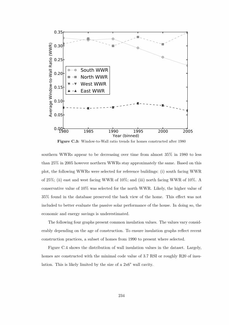
1980 1985 1990 1995 2000 2005Year (binned)

0.00

0.05

0.10

0.15

0.20

0.25

0.30

0.35

AverageWindow-to-W

allRatio(W

WR)

South WWR

North WWR

West WWR

East WWR

Figure C.3: Window-to-Wall ratio trends for homes constructed after 1980

southern WWRs appear to be decreasing over time from almost 35% in 1980 to less

than 25% in 2005 however northern WWRs stay approximately the same. Based on this

plot, the following WWRs were selected for reference buildings: (i) south facing WWR

of 25%; (ii) east and west facing WWR of 10%; and (iii) north facing WWR of 10%. A

conservative value of 10% was selected for the north WWR. Likely, the higher value of

35% found in the database preserved the back view of the home. This effect was not

included to better evaluate the passive solar performance of the house. In doing so, the

economic and energy savings is underestimated.

The following four graphs present common insulation values. The values vary consid-

erably depending on the age of construction. To ensure insulation graphs reflect recent

construction practices, a subset of homes from 1990 to present where selected.

Figure C.4 shows the distribution of wall insulation values in the dataset. Largely,

homes are constructed with the minimal code value of 3.7 RSI or roughly R20 of insu-

lation. This is likely limited by the size of a 2x6" wall cavity.

234

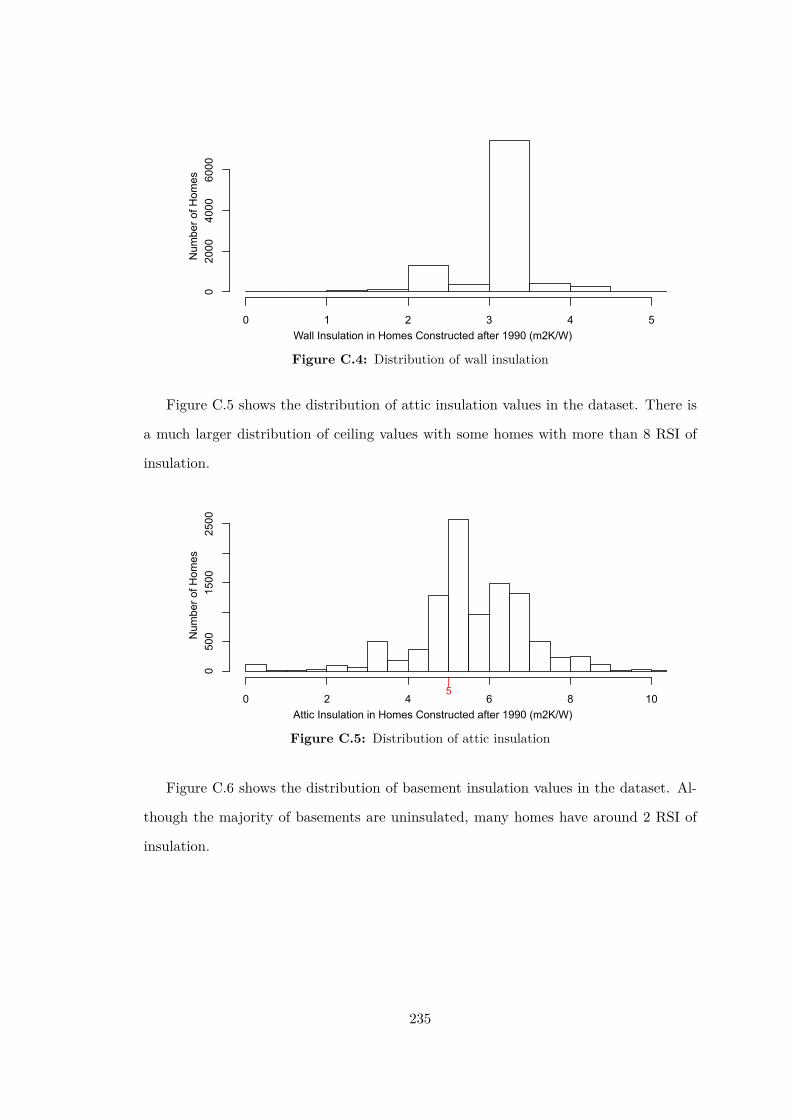
Wall Insulation in Homes Constructed after 1990 (m2K/W)

Num

ber o

f Hom

es

0 1 2 3 4 5

020

0040

0060

00

Figure C.4: Distribution of wall insulation

Figure C.5 shows the distribution of attic insulation values in the dataset. There is

a much larger distribution of ceiling values with some homes with more than 8 RSI of

insulation.

Attic Insulation in Homes Constructed after 1990 (m2K/W)

Num

ber o

f Hom

es

50 2 4 6 8 10

050

015

0025

00

Figure C.5: Distribution of attic insulation

Figure C.6 shows the distribution of basement insulation values in the dataset. Al-

though the majority of basements are uninsulated, many homes have around 2 RSI of

insulation.

235

Basement Wall Insulation in Homes Constructed after 1990 (m2K/W)

Num

ber o

f Hom

es

0 1 2 3 4 5 6

050

015

0025

00

Figure C.6: Distribution of basement wall insulation

Finally, figure C.7 shows the distribution of slab insulation values in the dataset. As

shown in this figure, the majority of homes in Canada have uninsulated basement slabs.

Basement Slab Insulation in Homes Constructed after 1990 (m2K/W)

Num

ber o

f Hom

es

0 1 2 3 4 5 6

020

0040

0060

00

Figure C.7: Distribution of slab insulation

Table C.1 shows construction values recommended by various codes and standards

and summarizes values from the NRCan dataset.

236

Table C.1: Code requirements for reference building

MNECH-1997 ASHRAE90.2-2007

EnergyStar NRCanDataset

ValueUsed

Attic Insulation (m2K/W ) 8.8 8.6 7.7 5 8.8Wall Insulation (m2K/W ) 4.4 3.7 3.8 3.5 4.4Below-grade walls (m2K/W ) 3.5 1.4 1.7 1.7 3.5Below-grade slab (m2K/W ) 1.9 – 0.88 0 1.9Envelope Tightness (ACH@50Pa) – – 2.5 3.5 3.5

When selecting reference building values, first energy standards were considered.

However, values from the NRCan dataset were used if energy standard values were

not common. For example, consider insulation values for slabs. Although standards

recommended values of 0.8 to 1.9 RSI, these rarely found in the NRCan dataset. However

it might be that insulation of slabs is difficult to ascertain for energy auditors so energy

standards were used for slab insulation. Although present building codes specify 8.8 RSI

of attic insulation, this would not commonly found in the NRCan dataset. This likely

due to settling of blown-in insulation or deterioration of existing value. Regardless, a

value of 8.8 RSI from standards was used for ceiling insulation.

237

Pathways to Net-Zero Energy Buildings: An Optimization ... · ABSTRACT Pathways to Net-Zero Energy...

Documents

Transcript of Pathways to Net-Zero Energy Buildings: An Optimization ... · ABSTRACT Pathways to Net-Zero Energy...