
Path-Specific Propagation Models for Subgroup 3K-1 Propagation Models for Subgroup 3K-1 ... specific...
71
Path-Specific Propagation Models for Subgroup 3K-1 Paul McKenna, NTIA/ITS.E 1 Alakananda Paul, NTIA/OSM 2 National Telecommunications and Information Administration 1 Mr. McKenna is with the Institute for Telecommunication Sciences, Boulder, CO 2 Dr. Alakananda Paul is with the Office of Spectrum Management, Washington, D.C.
Transcript of Path-Specific Propagation Models for Subgroup 3K-1 Propagation Models for Subgroup 3K-1 ... specific...

Path-Specific Propagation Models for Subgroup 3K-1
Paul McKenna, NTIA/ITS.E1
Alakananda Paul, NTIA/OSM2
National Telecommunications and Information Administration1Mr. McKenna is with the Institute for Telecommunication Sciences,
Boulder, CO2Dr. Alakananda Paul is with the Office of Spectrum Management,
Washington, D.C.

Introduction and Background
•
Six Path-Specific Models were proposed for study–
Each has a somewhat different rationale but a “common”
goal
–
Each is intended to optimize the radio propagation prediction on most paths
–
The optimal model will choose the “best”
parts of each model

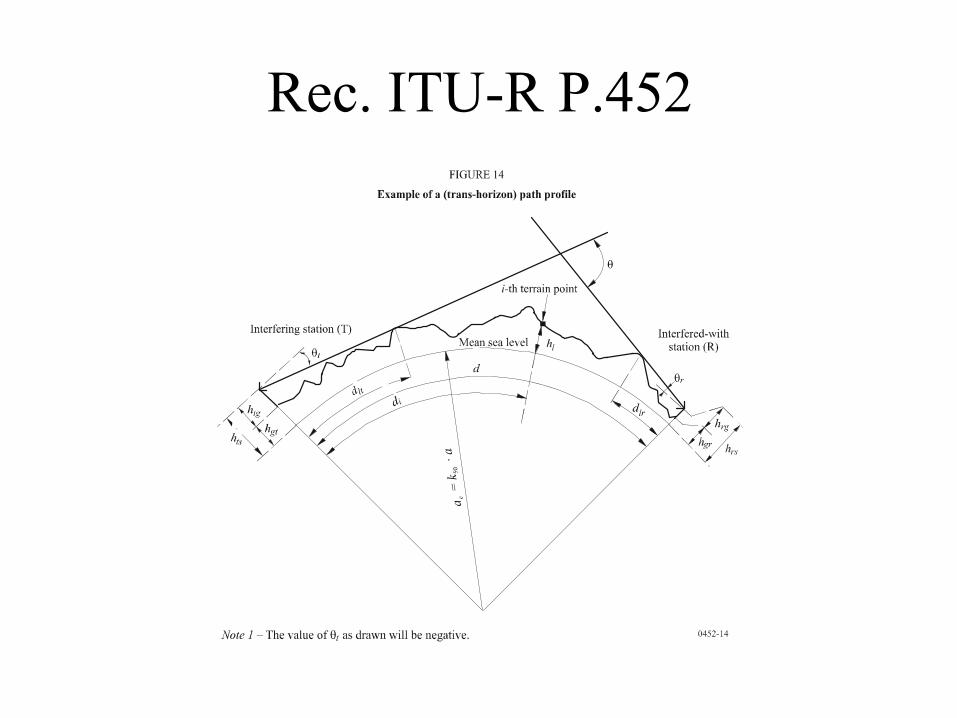
Rec. ITU-R P.452
•
Clear Air Propagation Mechanisms– line-of-sight (including signal enhancements due to
multipath and focusing effects);– diffraction (embracing smooth-earth, irregular terrain
and sub-path cases);– tropospheric scatter;– anomalous propagation (ducting and layer
reflection/refraction);– height-gain variation in clutter (where relevant).
Rec. ITU-R P.452

Rec. ITU-R P.452•
Line-of-SightLb0
(p)
=
92.5
+
20 log(fd )+
Es (
p) + Ag dBwhere:Es (p)
: correction for multipath and focusing effects:Es (p) = 2.6 (1 –
e–
d / 10)log(p/50)
dBAg : total gaseous absorption (dB):
Ag
=[γo
+γw
(ρ)]dwhere:γo , γw (ρ)
: specific attenuation due to dry air and water vapor, respectively, and are found from the equations in Recommendation
ITU-R
P.676ρ
: water vapor density:ρ=7.5+2.5ω
g/m3
ω
:
fraction of the total path over
water.

Rec. ITU-R P.452
•
Diffraction
)50
log()1(6.2)(
)()()log(205.92)(100
100)(
%)]50()()[(%)50()(
10/)(
0
0
pepE
ApEpLdfpL
I
pIpF
LLpFLpL
lrlt ddsd
gsddbd
i
ddidd
+−−=
+++⋅+=
⎟⎠⎞
⎜⎝⎛
⎟⎠⎞
⎜⎝⎛
=
−+=
β
β

Rec. ITU-R P.452•
Obstacle Height Above the Straight Line Between the Ends of the Path
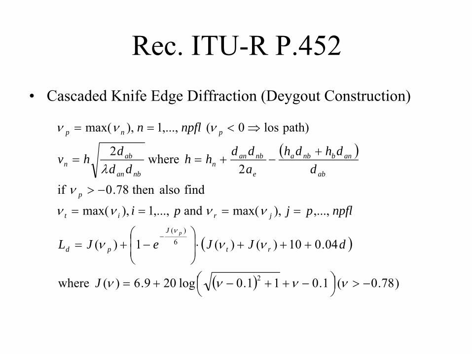
Rec. ITU-R P.452•
Cascaded Knife Edge Diffraction (Deygout Construction)
( )
( )
( ) )78.0( 1.011.0log209.6)( where
04.010)()(1)(
,...,),max( and ,...,1),max(
find also then 78.0 if2
where2
path) los 0( ,...,1 ),max(
2
6)(
−>⎟⎠⎞⎜
⎝⎛ −++−+=
+++⋅⎟⎟⎠
⎞⎜⎜⎝
⎛−+=
====
−>
+−+==
⇒<==
−
νννν
ννν
νννν
νλ
ννν
ν
J
dJJeJL
npflpjpi
ddhdh
addhh
dddhv
npfln
rt
J
pd
jrit
p
ab
anbnba
e
nbann
nban
abn
pnp
p

Rec. ITU-R P.452
•
Tropospheric Scatter
rte
GGc
f
gcfbs
ad
eL
ffL
pALNdLpL
rt
θθθ
θ
++=
⋅=
⎟⎟⎠
⎞⎜⎜⎝
⎛⎟⎠⎞
⎜⎝⎛−=
⎟⎟⎠
⎞⎜⎜⎝
⎛⎟⎟⎠
⎞⎜⎜⎝
⎛−++−+++=
+
3
)(055.0
2
7.0
0
10051.0
2log5.2log25
50log1.1015.0573.0log20190)(

Rec. ITU-R P.452
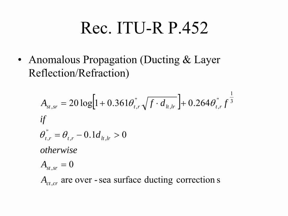
•
Anomalous Propagation (Ducting & Layer Reflection/Refraction)
),)(log()correction roughnessterrain ()correctiongeometry path (
)(12)log()107.32.1(12)(
)1.0,min()1.0,min(10
)(105)(
))(log(2045.102
)()(
0
3
3
3/15
d
ppdpA
dda
d
pAfapA
AAAAddfA
ApAApL
lrrltte
ed
crctsrstlrltf
gdfba
βββ
ββ
θθθ
θ
Γ=Γ⋅⋅=
+⋅++−=
++=′
+′⋅=
++++++=
++=
Γ−
−
Rec. ITU-R P.452
•
Anomalous Propagation (Ducting & Layer Reflection/Refraction)
[ ]
scorrection ducting surface sea-over are 0
01.0
264.0361.01log20
,
,
,,'',
31
'',,
'',,
crct
srst
lrltrtrt
rtlrltrtsrst
AAotherwise
dif
fdfA
=
>−=
+⋅+=
θθ
θθ
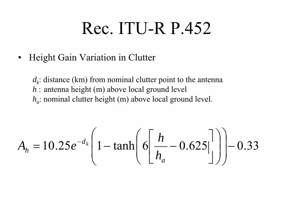
Rec. ITU-R P.452•
Height Gain Variation in Clutter
dk : distance (km) from nominal clutter point to the antenna h :
antenna height (m) above local ground levelha : nominal clutter height (m) above local ground level.
33.0625.06tanh125.10 −⎟⎟⎠
⎞⎜⎜⎝
⎛⎟⎟⎠
⎞⎜⎜⎝
⎛⎥⎦
⎤⎢⎣
⎡−−= −
a
dh h
heA k

Rec. ITU-R P.452TABLE 6
Nominal clutter heights and distances
Clutter (ground-cover) category Nominal height, ha (m)
Nominal distance, dk(km)
High crop fields Park land Irregularly spaced sparse trees Orchard (regularly spaced) Sparse houses
4
0.1
Village centre 5 0.07 Deciduous trees (irregularly spaced) Deciduous trees (regularly spaced) Mixed tree forest
15
0.05
Coniferous trees (irregularly spaced) Coniferous trees (regularly spaced)
20 0.05
Tropical rain forest 20 0.03
Suburban 9 0.025
Dense suburban 12 0.02
Urban 20 0.02
Dense urban 25 0.02
Industrial zone 20 0.05
Rec. ITU-R P.452-12
•
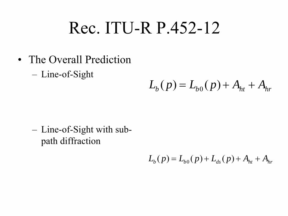
The Overall Prediction–
Line-of-Sight
–
Line-of-Sight with sub- path diffraction
hrhtbb AApLpL ++= )()( 0
hrhtdsbb AApLpLpL +++= )()()( 0

Rec. ITU-R P.452-12
•
The Overall Prediction–
Trans-horizon
( )
( ) ( )
( )[ ]
( ) hrhtpLpLpL
b
jibibd
jkbdk
pLpL
bam
jk
AApL
FpFLpFL
FdFpLdFeepL
FddF
bdbambs
bba
++++⋅−=
⋅⋅+−⋅+
−⋅⎥⎥⎦
⎤
⎢⎢⎣
⎡⋅+−⋅⎟⎟
⎠
⎞⎜⎜⎝
⎛+=
⎟⎟⎠
⎞⎜⎜⎝
⎛⎟⎠⎞
⎜⎝⎛ −
+⋅−=⎟⎟⎠
⎞⎜⎜⎝
⎛⎟⎠⎞
⎜⎝⎛ −
+⋅−=
−−− )(2.0)(2.0)(2.0
00
5.2)(
5.2)(
101010log0.5)(
)()()()(1%)50(
)(1)()()(1ln5.2)(
3.0)3.0(4.2tanh15.01)(,
20205.1tanh15.01)(
0
θβ
θ
θθ
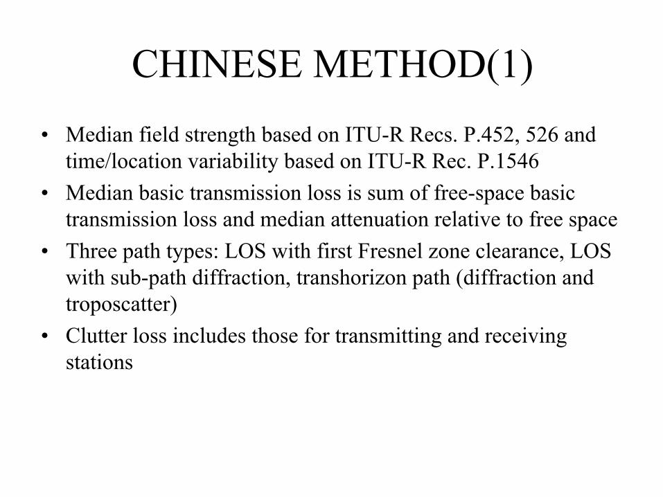
CHINESE METHOD(1)•
Median field strength based on ITU-R Recs. P.452, 526 and time/location variability based on ITU-R Rec. P.1546
•
Median basic transmission loss is sum of free-space basic transmission loss and median attenuation relative to free space
•
Three path types: LOS with first Fresnel zone clearance, LOS with sub-path diffraction, transhorizon path (diffraction and troposcatter)
•
Clutter loss includes those for transmitting and receiving stations
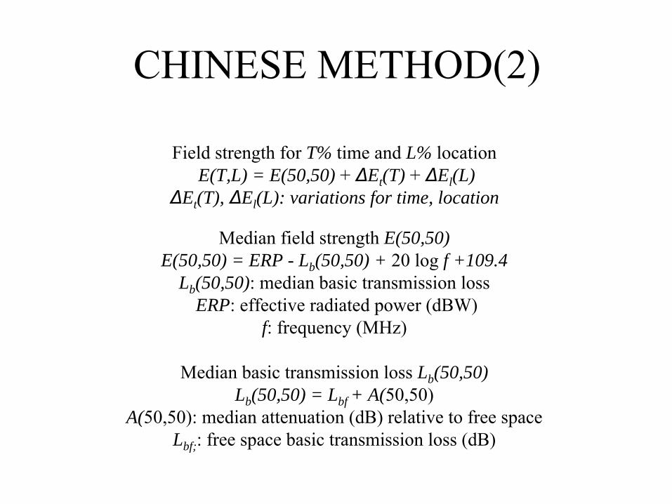
CHINESE METHOD(2)
Field strength for
T% time
and
L% locationE(T,L) = E(50,50) + ΔEt (T) + ΔEl (L)
ΔEt (T), ΔEl (L): variations for time, location
Median field strength E(50,50)E(50,50) = ERP - Lb (50,50) + 20 log
f +109.4Lb (50,50): median basic transmission loss
ERP: effective radiated power (dBW)f: frequency (MHz)
Median basic transmission loss
Lb (50,50) Lb (50,50) = Lbf + A(50,50)
A(50,50): median attenuation (dB) relative to free spaceLbf; : free space basic transmission loss (dB)

CHINESE METHOD(3)LOS path with first Fresnel zone clearance
Lb (50,50) = Lbf + Acldt + Acldr
Acldt , Acldr : additional clutter losses due to diffraction
LOS path with sub-path diffractionLb (50,50) = Lbf + Acldt + Acldr + Ad (50,50)
Ad (50,50): median sub-path diffraction loss (P.526)
Trans-horizon pathLb (50,50) = -10 log {10-0.1L
bd(50,50)
+ 10-0.1Lbs
(50,50)}Lbd : median basic transmission loss due to trans-horizon diffraction
Lbs : median basic transmission loss due to troposcatter
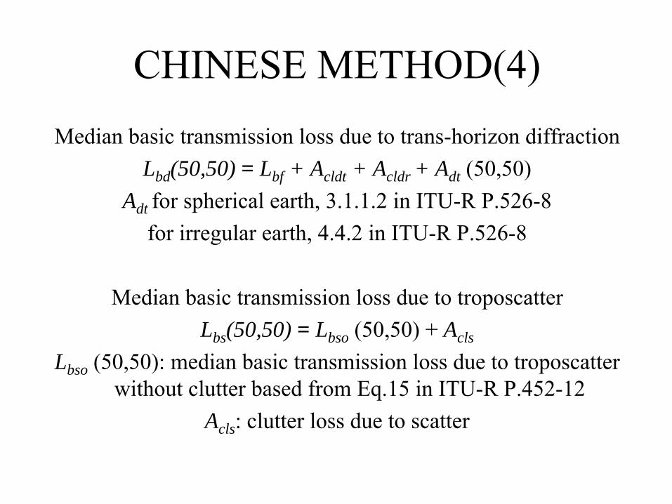
CHINESE METHOD(4)Median basic transmission loss due to trans-horizon diffraction
Lbd (50,50) = Lbf + Acldt + Acldr + Adt (50,50)Adt for spherical earth, 3.1.1.2 in ITU-R P.526-8
for irregular earth, 4.4.2 in ITU-R P.526-8
Median basic transmission loss due to troposcatterLbs (50,50) = Lbso (50,50) + Acls
Lbso (50,50): median basic transmission loss due to troposcatter without clutter based from Eq.15 in ITU-R P.452-12
Acls : clutter loss due to scatter
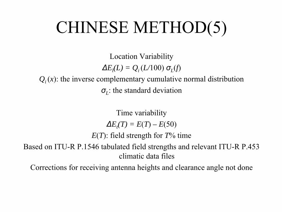
CHINESE METHOD(5)Location Variability
ΔEl (L) = Qi (L/100) σL (f)Qi (x): the inverse complementary cumulative normal distribution
σL : the standard deviation
Time variabilityΔEt (T) = E(T)
– E(50)E(T): field strength for T% time
Based on ITU-R P.1546 tabulated field strengths and relevant ITU-R P.453 climatic data files
Corrections for receiving antenna heights and clearance angle not done

PSPROGCN-1•
FUNCTION E50 (F,ERP,NPL,HTG,HRG,N,HI,DI,NGC,HGC,ALON1,ALAT1, ALON2,ALAT2) for calculation of the median field strength
•
FUNCTION DETT (F,T,HTG,N,HI,DI,GNC,ALON1,ALAT1,ALON2,ALAT2)for calculation of the variation with time
•
FUNCTION ETQ (F,ERP,NPL,HTG,HRG,N,HI,DI,NGC,HGC,ALON1,ALAT1, ALON2,ALAT2,T,Q)for calculating of field strength for any time and location percentages

PSPROGCN-1
•
FILES DNZ.TXT,NO.TXT,IDN.TXT AND FST.TXT filesfor basic climatic and field strength data
•
MAIN PROGRAMfor opening the basic climatic and field strength data files and the measurement data files, reading and processing the data, calculating field strength and comparing it with measured field strength, and putting the results into the output data file

PSPROGCN-1Input Parameters•
frequency
•
effective radiated power•
polarization
•
antenna heights above ground level•
distance from transmitting/base station, terrain height amsl, ground cover type and its height at the ith
terrain point on the
path profile•
latitude and longitude of transmitting/base station
•
latitude and longitude of receiving/mobile station•
percentage of time

EBU METHOD(1) Propagation Mechanisms
•
Free space•
Diffraction loss (irregular terrain and sub-path
•
Tropospheric scatter•
Anomalous propagation (ducting)
•
Height variation in ground cover•
Building penetration

EBU METHOD(2) Basic Input Data
Parameter Description
f Frequency (MHz)
p Required time percentage(s) for which the basic transmission loss is not exceeded
φt
φr Latitude of transmitter and receiver (degrees)
ψt
ψr Longitude of transmitter and receiver (degrees)
htg
hrg Transmitter and receiver antenna center height above ground level (m)
hts
hrs Transmitter and receiver antenna center height above mean sea level (m)
Gt
Gr Transmitter and receiver antenna gain in the direction of horizon along great circle path
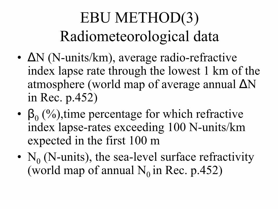
EBU METHOD(3) Radiometeorological data
•
ΔN (N-units/km), average radio-refractive index lapse rate through the lowest 1 km of the atmosphere (world map of average annual ΔN in Rec. p.452)
•
β0
(%),time percentage for which refractive index lapse-rates exceeding 100 N-units/km expected in the first 100 m
•
N0
(N-units), the sea-level surface refractivity (world map of annual N0 in Rec. p.452)

EBU METHOD(4) Parameters derived from path profile analysis
Path type Parameter Description
Transhorizon d Great-circle path distance in km
Transhorizon dlt
dlr Distance from transmit and receive antennas to their respective horizons in km
Transhorizon θt
θr Transmit and receive horizon elevation angles
Transhorizon θ Path angular distance
All hts
hrs Antenna center height above mean sea level

EBU METHOD(5) Path classifications and propagation models
LOS with first Fresnel zone clearance•
Free space basic transmission loss
•
Relative ground cover and receiving antenna height loss
•
Building penetration loss (where appropriate)
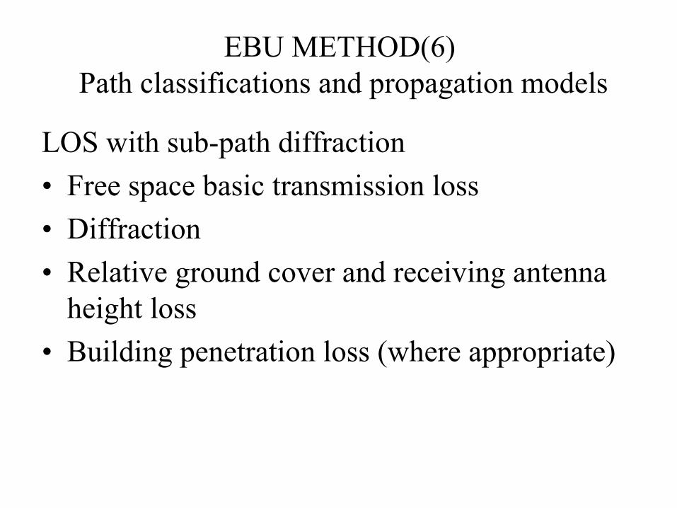
EBU METHOD(6) Path classifications and propagation models
LOS with sub-path diffraction•
Free space basic transmission loss
•
Diffraction•
Relative ground cover and receiving antenna height loss
•
Building penetration loss (where appropriate)
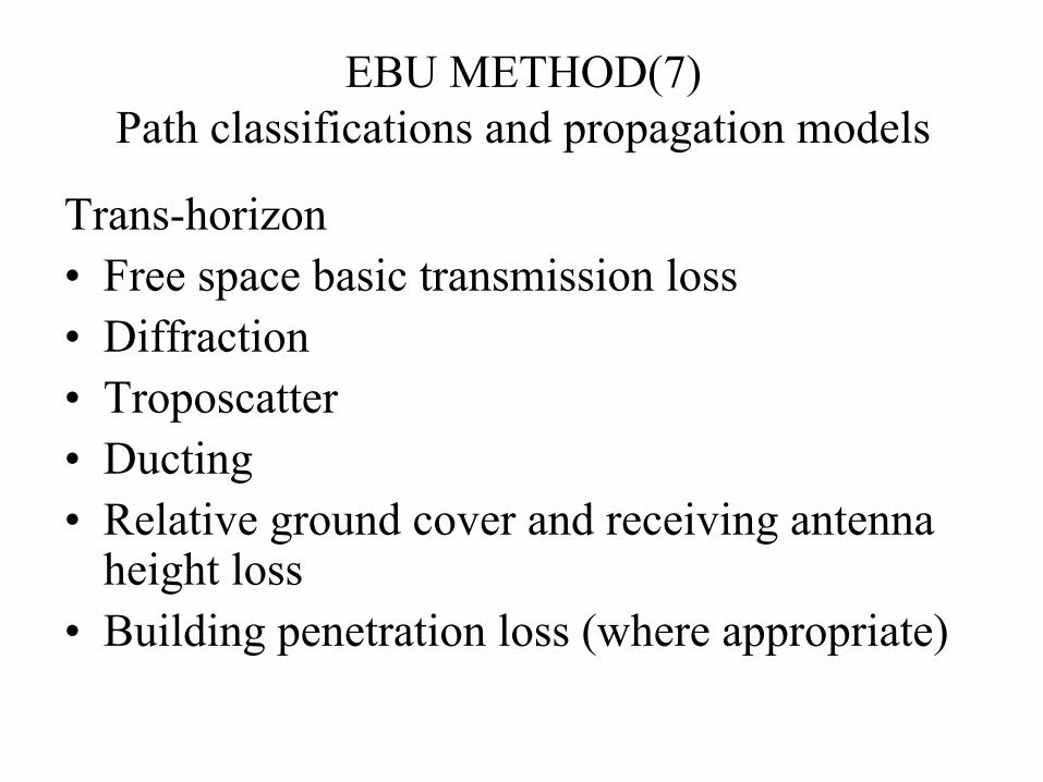
EBU METHOD(7) Path classifications and propagation models
Trans-horizon•
Free space basic transmission loss
•
Diffraction•
Troposcatter
•
Ducting•
Relative ground cover and receiving antenna height loss
•
Building penetration loss (where appropriate)

EBU METHOD(7.1)
Electric field strength for 1 kW e.r.p Eb = 139
– Lb + 20 log
f dBμV/m
Lb is basic transmission loss in dBFree space basic transmission lossLbf = 32.4 +20 log f + 20 log d dB
Diffraction lossBased on ITU-R P.452 and P.526
Assumes a horizontal exclusion zone of the principal obstacle to avoid over-estimating loss
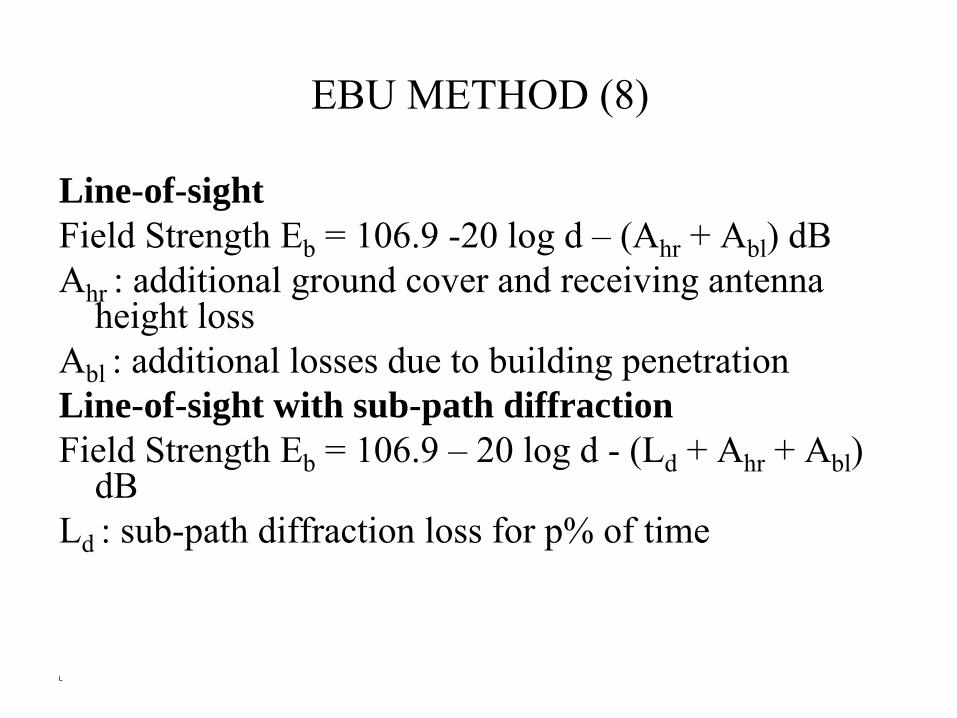
EBU METHOD (8)
Line-of-sightField Strength Eb
= 106.9 -20 log d –
(Ahr
+ Abl
) dB Ahr : additional ground cover and receiving antenna
height lossAbl : additional losses due to building penetrationLine-of-sight with sub-path diffractionField Strength Eb
= 106.9 –
20 log d -
(Ld
+ Ahr
+ Abl
) dB
Ld : sub-path diffraction loss for p% of time
L

EBU METHOD (9)
Trans-horizonEb
= 10 log(10Ed/10
+10Es/10
+ 10Ea/10) –
(Ahr
+ Abl
) Ed
= 106.9 –
20 log d –
LdLd
: diffraction loss for p% of timeEs
= 106.9 –
20 log d –
LsLs : troposcatter loss for p% of timeEa
: field strength resulting from ducting

SWISS STUDY•
Comparison of predicted results with measured data in Alpine region
•
Three diffraction modeling techniques: Bullington, Epstein-Peterson and Deygout methods and Longley-
Rice model used•
Terrain profile from DBSG5 and Shuttle Radar Topography Mission (SRTM) data
•
Bullington method gives consistently optimistic results with relatively small errors, other methods overestimate path loss with larger errors

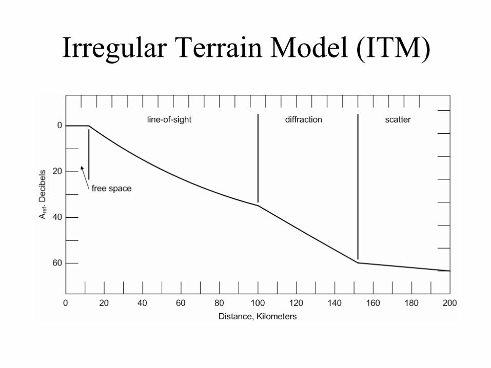
Irregular Terrain Model (ITM)
•
Computed Reference Attenuation (Attenuation Relative to Free Space)
xlsref
xses
xlsded
lsls
kkelref
dddAdddmA
ddddmA
ddddadaaA
,at continuous is for for
for )ln,0max( 21
=>+=
≤<+=
≤⎟⎟⎠
⎞⎜⎜⎝
⎛++=
Irregular Terrain Model (ITM)

Irregular Terrain Model (ITM)•
Time, Location and Situation Variabilities; Attenuation not exceeded for pT (percentage Time), pL
(percentage Locations) and pS
(percentage Situations), A(pT
,pL
,pS
):
( ) ( )
( ) ( )
( ) ( )
( )
0 if 1029
29
0 if ,,
deviation standard theis andmean theis where usingthen 21 and )( where
100,
100,
100)(),(),(,,
''
''
''
'00
1 2
<⋅−
−=
≥=
−−−−=
⋅+=
===
⎟⎟⎠
⎞⎜⎜⎝
⎛⎟⎠⎞
⎜⎝⎛
⎟⎠⎞
⎜⎝⎛
⎟⎠⎞
⎜⎝⎛=≡
∫∞
−−
AA
AA
AAzzzA
YYYVAA
XqzXqX
dtezQqqQqz
pzpzpzAqzqzqzAzzzA
SLT
SLTmedref
z
t
SLTSLTSLT
σσπ

Irregular Terrain Model (ITM)
•
Coefficients for the Diffraction Range
( )
3334
34
44
33
34
3
31
31
2
,
)(
)(7574.2
3787.1,max2
2
dmAAddAAm
dAA
dAAXdd
Xdddda
aa
X
dedd
diff
diff
ae
aelrltls
ee
eae
−=−−
=
=
=+=
++=
⎟⎟⎠
⎞⎜⎜⎝
⎛=⎟⎟
⎠
⎞⎜⎜⎝
⎛=
−
πλ
λπ
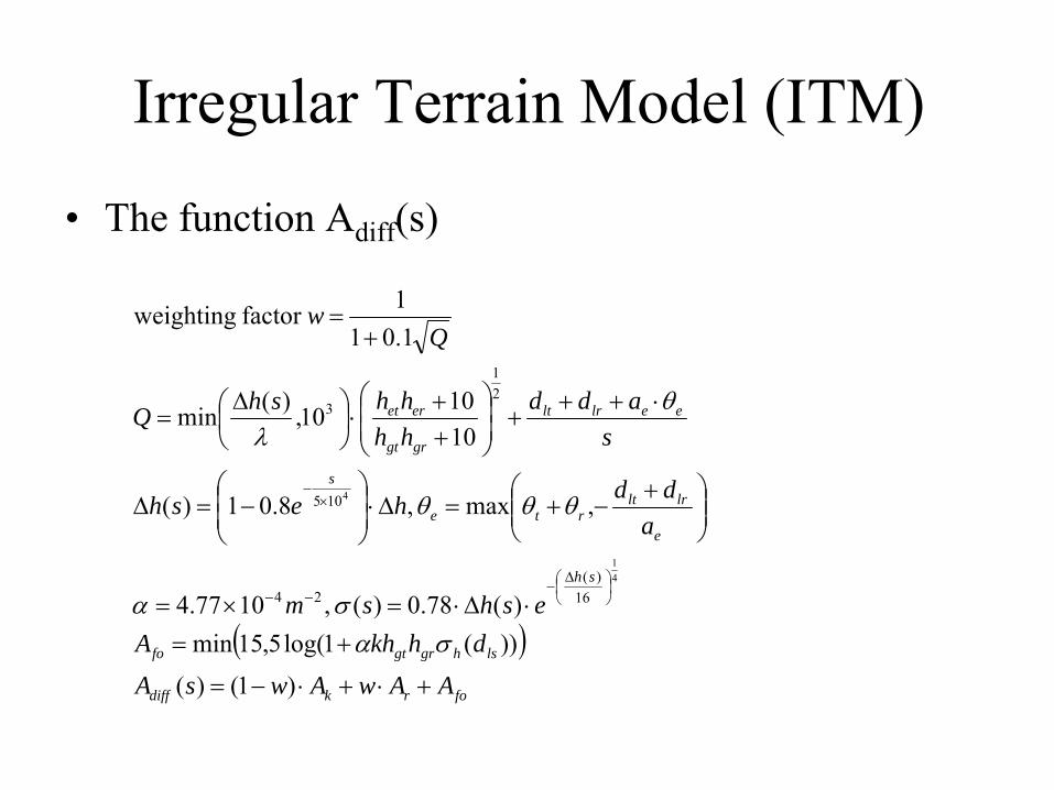
Irregular Terrain Model (ITM)
•
The function Adiff
(s)
( )forkdiff
lshgrgtfo
sh
e
lrltrte
s
eelrlt
grgt
eret
AAwAwsA
dhkhAeshsm
addhesh
sadd
hhhhshQ
Qw
+⋅+⋅−=
+=⋅Δ⋅=×=
⎟⎟⎠
⎞⎜⎜⎝
⎛ +−+=Δ⋅⎟
⎟⎠
⎞⎜⎜⎝
⎛−=Δ
⋅+++⎟
⎟⎠
⎞⎜⎜⎝
⎛
++
⋅⎟⎠⎞
⎜⎝⎛ Δ=
+=
⎟⎠⎞
⎜⎝⎛ Δ−
−−
×−
)1()(
))(1log(5,15min)(78.0)( ,1077.4
,max ,8.01)(
101010,)(min
1.011factor weighting
41
4
16)(
24
105
21
3
σασα
θθθ
θλ
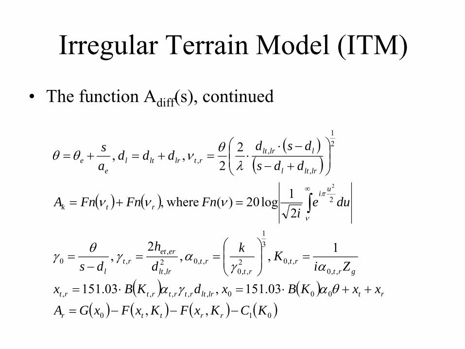
Irregular Terrain Model (ITM)
•
The function Adiff
(s), continued
( )( )
( ) ( )
( ) ( )( ) ( ) ( ) ( )010
000,,,,,
,,0,,0
31
2,,0
,,02,
,,0
2
21
,
,,
,,03.151 ,03.151
1 , ,2
,
21log20)( where,
22
, ,
2
KCKxFKxFxGAxxKBxdKBx
ZiKk
dh
ds
duei
FnFnFnA
ddsdsd
dddas
rrttr
rtlrltrtrtrtrt
grtrt
rtrt
lrlt
eretrt
l
ui
rtk
lrltl
llrltrtlrltl
ee
−−−=
++⋅=⋅=
=⎟⎟⎠
⎞⎜⎜⎝
⎛==
−=
=+=
⎟⎟⎠
⎞⎜⎜⎝
⎛
+−−⋅
⋅=+=+=
∫∞
θαγα
αγαγθγ
ννν
λθνθθ
ν
π

Irregular Terrain Model (ITM)
Irregular Terrain Model (ITM)
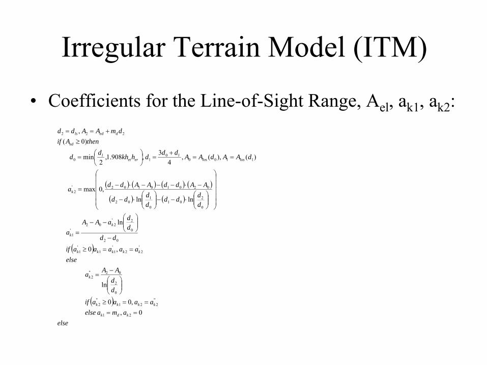
•
Coefficients for the Line-of-Sight Range, Ael
, ak1
, ak2
:
( ) ( ) ( ) ( )
( ) ( )
( )
( )
elseamaelse
aaaaif
dd
AAa
elseaaaaaif
ddddaAA
a
dddd
dddd
AAddAAdda
dAAdAAdddhkhdd
thenAifdmAAdd
kdk
kkkk
k
kkkkk
k
k
k
loslosl
eretl
ed
dedls
0 , ,00
ln
,0
ln
lnln,0max
)( ),(,4
3 ,908.1,2
min
)0( ,
21
"221
"2
0
2
02"2
'22
'11
'1
02
0
2'202
'1
0
201
0
102
02010102'2
11000
10
222
====≥
⎟⎟⎠
⎞⎜⎜⎝
⎛−
=
==≥
−
⎟⎟⎠
⎞⎜⎜⎝
⎛−−
=
⎟⎟⎟⎟⎟
⎠
⎞
⎜⎜⎜⎜⎜
⎝
⎛
⎟⎟⎠
⎞⎜⎜⎝
⎛⋅−−⎟⎟
⎠
⎞⎜⎜⎝
⎛⋅−
−⋅−−−⋅−=
==+
=⎟⎠⎞
⎜⎝⎛=
≥+==
Irregular Terrain Model (ITM)
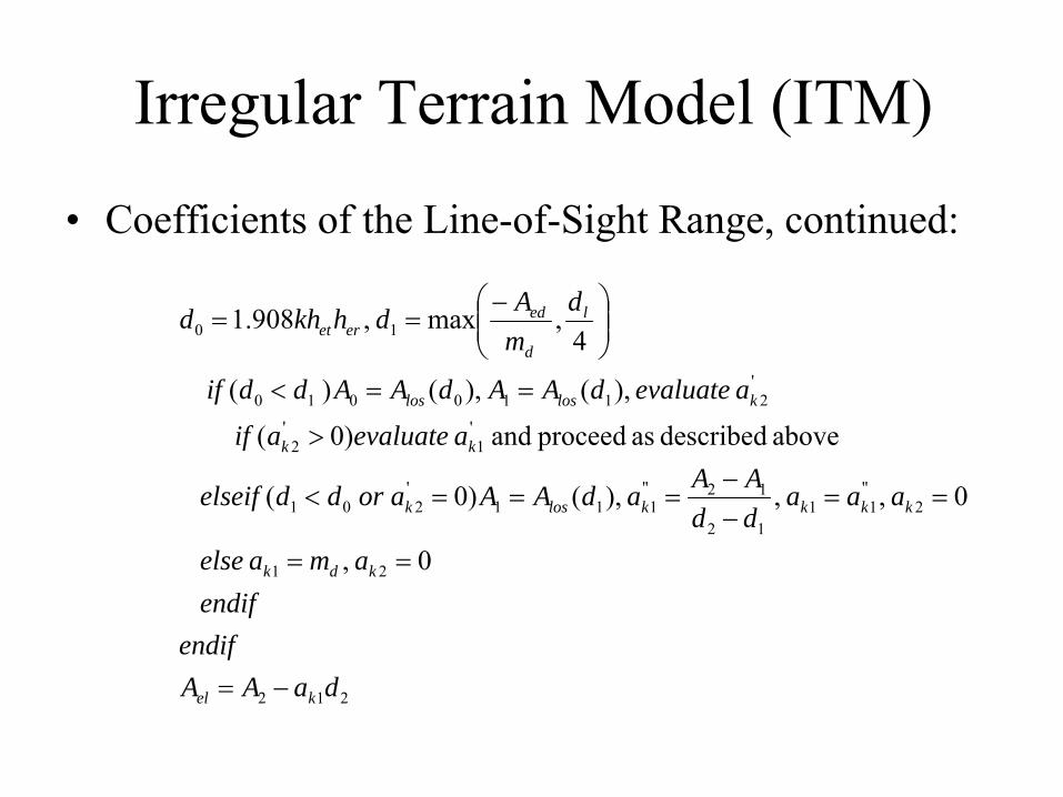
•
Coefficients of the Line-of-Sight Range, continued:
212
21
2"11
12
12"111
'201
'1
'2
'2110010
10
0 ,
0 , , ),()0 (
above described as proceed and )0(
),( ),() (
4,max ,908.1
daAAendif
endifamaelse
aaaddAAadAAaorddelseif
aevaluateaif
aevaluatedAAdAAddif
dmAdhkhd
kel
kdk
kkkklosk
kk
kloslos
l
d
ederet
−=
==
==−−
===<
>
==<
⎟⎟⎠
⎞⎜⎜⎝
⎛ −==
Irregular Terrain Model (ITM)
•
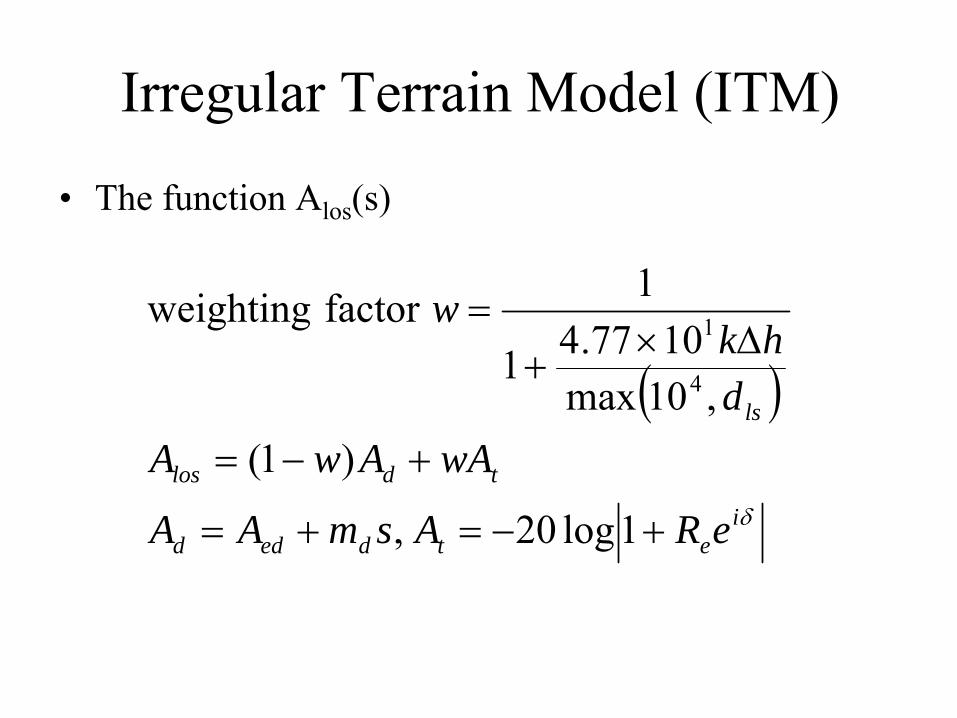
The function Alos
(s)
( )
δietdedd
tdlos
ls
eRAsmAA
wAAwAd
hkw
+−=+=
+−=
Δ×+
=
1log20 ,
)1(,10max
1077.41
1factor weighting
4
1
Irregular Terrain Model (ITM)
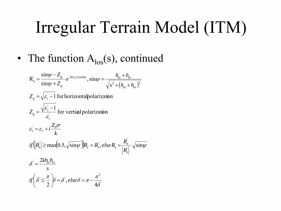
•
The function Alos
(s), continued
( )
( )( )
'
2''
'
'
'''
0'
'
'
g
'
22
sin)('e
4 ,
2
2
sin ,sin,5.0max
onpolarizati alfor vertic 1
Z
onpolarizati horizontalfor 1
sin ,sinsin
R
δππδδδπδ
δ
ψψ
σεε
εε
ε
ψψψ ψσ
−==⎟⎠⎞
⎜⎝⎛ ≤
=
⋅==≥
+=
−=
−=
++
+=⋅
+−
= −
elseif
shkh
RRRelseRRRif
kZi
Z
hhs
hheZZ
eret
e
eeeee
rr
r
r
rg
eret
eretsk
g
g h

Irregular Terrain Model (ITM)
•
Coefficients of the (Tropo)Scatter Range
( )
( ) ⎟⎟⎠
⎞⎜⎜⎝
⎛−−−
×⋅+=
−+=×−
=
==×+=×+=
sd
sedaellsx
xsdedes
s
scatscat
l
mmdmAAkXddd
dmmAA
AAm
dAAdAAdddd
551
556
6655
556
55
,1077.4log,max
where,102
)( ),(102 ,102
Irregular Terrain Model (ITM)
•
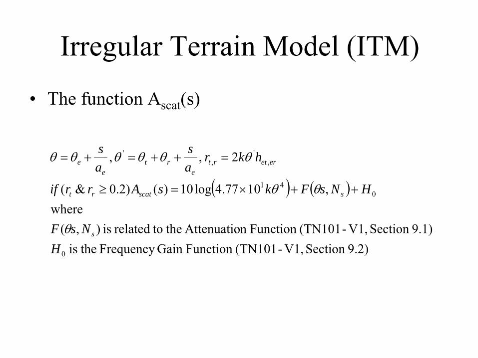
The function Ascat
(s)
( ) ( )
9.2)Section V1,-(TN101Function Gain Frequency theis 9.1)Section V1,-(TN101Function n Attenuatio the torelated is ),(
where,1077.4log10)()2.0&(
2 , ,
0
041
,'
,'
HNsF
HNsFksArrif
hkras
as
s
sscatrt
eretrte
rte
e
θ
θθ
θθθθθθ
++×=≥
=++=+=
Irregular Terrain Model (ITM)
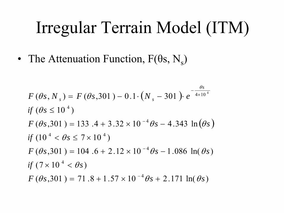
•
The Attenuation Function, F(θs, Ns
)
( )
( )
)ln(171.21057.18.71)301,()107(
)ln(086.11012.26.104)301,()10710(
ln343.41032.34.133)301,()10(
3011.0)301,(),(
4
4
4
44
4
4
104 4
sssFsif
sssFsif
sssFsif
eNsFNsFs
ss
θθθ
θ
θθθ
θ
θθθ
θ
θθθ
+×+=
<×
−×+=
×≤<
−×+=
≤
⋅−⋅−=
−
−
−
×−
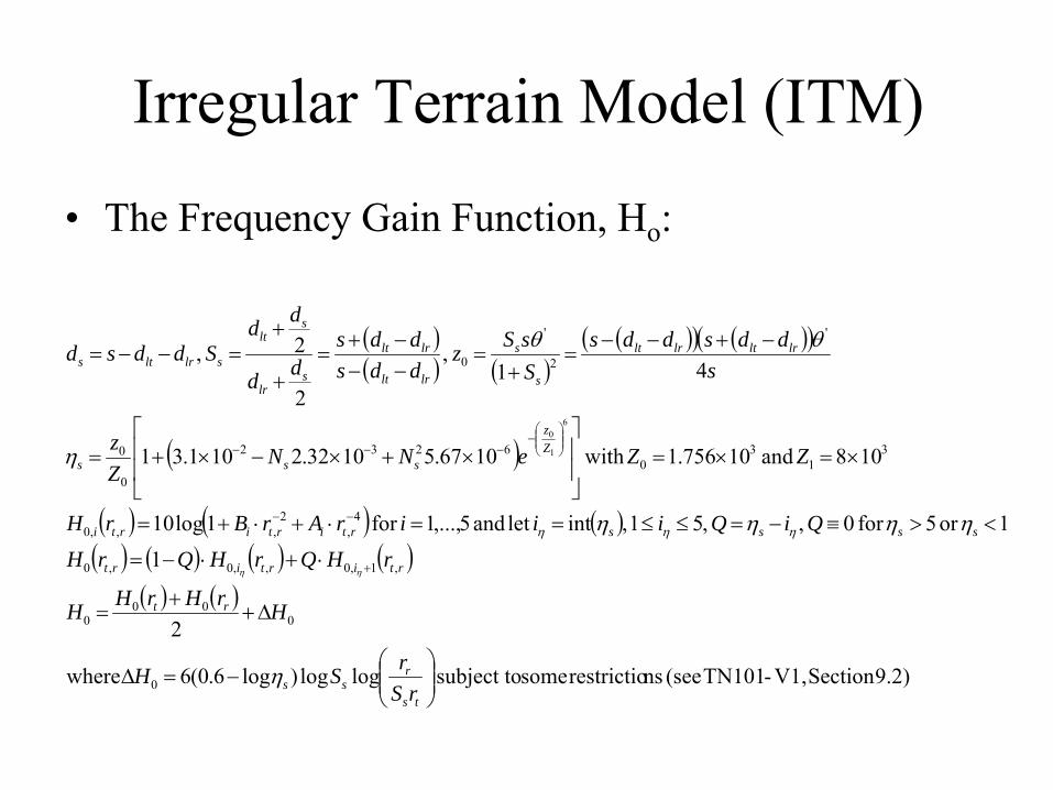
Irregular Terrain Model (ITM)
•
The Frequency Gain Function, Ho
:
( )( ) ( )
( )( ) ( )( )
( )
( ) ( ) ( )( ) ( ) ( ) ( )
( ) ( )
9.2)Section V1,-TN101 (see nsrestrictio some subject to loglog)log6.0(6 where
2
11or 5for 0 , ,51 ,intlet and 5,...,1for 1log10
108 and 10756.1 with 1067.51032.2101.31
41 ,
2
2 ,
0
000
0
,1,0,,0,0
4,
2,,,0
31
30
6232
0
0
'
2
'
0
6
1
0
⎟⎟⎠
⎞⎜⎜⎝
⎛−=Δ
Δ++
=
⋅+⋅−=
<>≡−=≤≤==⋅+⋅+=
×=×=⎥⎥
⎦
⎤
⎢⎢
⎣
⎡×+×−×+=
−+−−=
+=
−−−+
=+
+=−−=
+
−−
⎟⎟⎠
⎞⎜⎜⎝
⎛−
−−−
ts
rss
rt
rtirtirt
ssssrtirtirti
Zz
sss
lrltlrlt
s
s
lrlt
lrlt
slr
slt
slrlts
rSrSH
HrHrHH
rHQrHQrHQiQiiirArBrH
ZZeNNZz
sddsdds
SsSz
ddsdds
dd
ddSddsd
η
ηηηη
η
θθ
ηη
ηηη
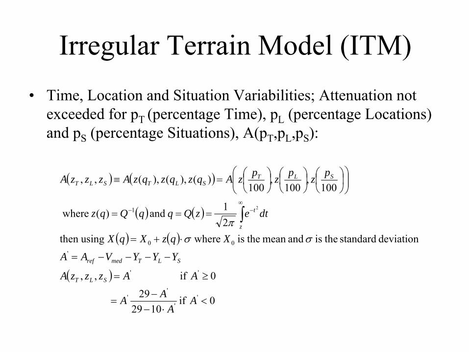
Irregular Terrain Model (ITM)•
Time, Location and Situation Variabilities; Attenuation not exceeded for pT (percentage Time), pL
(percentage Locations) and pS
(percentage Situations), A(pT
,pL
,pS
):
( ) ( )
( ) ( )
( ) ( )
( )
0 if 1029
29
0 if ,,
deviation standard theis andmean theis where usingthen 21 and )( where
100,
100,
100)(),(),(,,
''
''
''
'00
1 2
<⋅−
−=
≥=
−−−−=
⋅+=
===
⎟⎟⎠
⎞⎜⎜⎝
⎛⎟⎠⎞
⎜⎝⎛
⎟⎠⎞
⎜⎝⎛
⎟⎠⎞
⎜⎝⎛=≡
∫∞
−−
AA
AA
AAzzzA
YYYVAA
XqzXqX
dtezQqqQqz
pzpzpzAqzqzqzAzzzA
SLT
SLTmedref
z
t
SLTSLTSLT
σσπ

Irregular Terrain Model (ITM)
•
The Effective Distance for Variabilities, de
:
( )
exex
exex
e
eretex
dddd
ddddd
DakDahahad
>−+×=
≤×=
×=×=⋅++= −
for 103.1
for 103.1
10266.1 ,109 ,22
5
5
61
613
1
1111

Irregular Terrain Model (ITM)
•
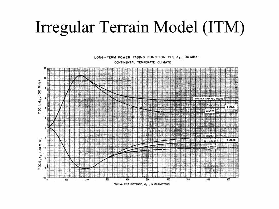
Time Variability, Vmed
(de
,clim):
Irregular Terrain Model (ITM)
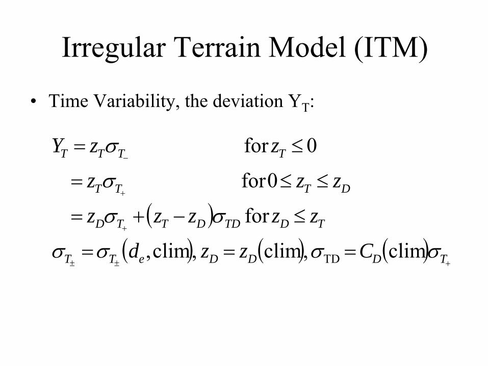
•
Time Variability, the deviation YT
:
( )( ) ( ) ( )
+±±
+
+
−
===
≤−+=
≤≤=
≤=
TDDDeTT
TDTDDTTD
DTTT
TTTT
Czzd
zzzzz
zzz
zzY
σσσσ
σσ
σ
σ
clim ,clim ,clim,
for
0for
0for
TD
Irregular Terrain Model (ITM)
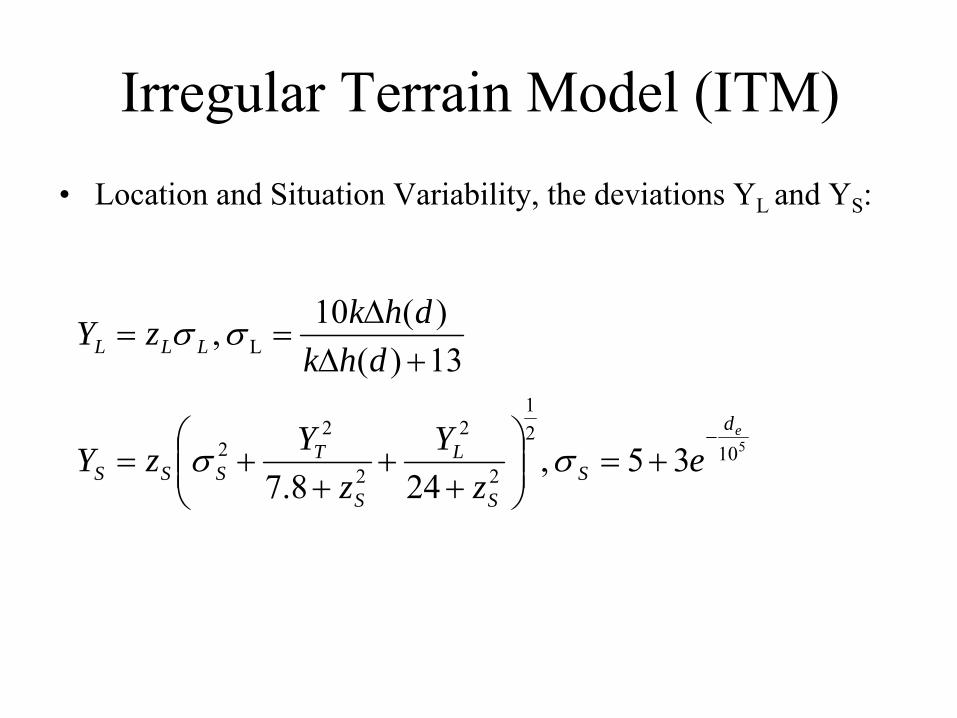
Irregular Terrain Model (ITM)•
Location and Situation Variability, the deviations YL and YS
:
51021
2
2
2
22
L
35 ,248.7
13)()(10 ,
ed
SS
L
S
TSSS
LLL
ez
Yz
YzY
dhkdhkzY
−+=⎟⎟
⎠
⎞⎜⎜⎝
⎛+
++
+=
+ΔΔ
==
σσ
σσ
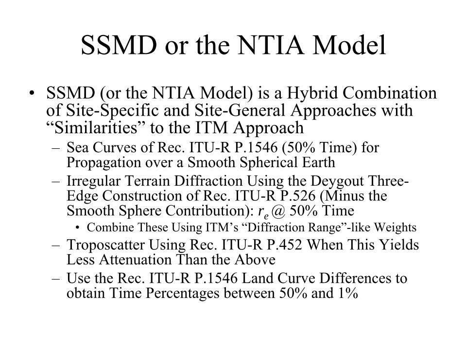
SSMD or the NTIA Model•
SSMD (or the NTIA Model) is a Hybrid Combination of Site-Specific and Site-General Approaches with “Similarities”
to the ITM Approach
–
Sea Curves of Rec. ITU-R P.1546 (50% Time) for Propagation over a Smooth Spherical Earth
–
Irregular Terrain Diffraction Using the Deygout Three- Edge Construction of Rec. ITU-R P.526 (Minus the
Smooth Sphere Contribution): re @ 50% Time•
Combine These Using ITM’s “Diffraction Range”-like Weights–
Troposcatter Using Rec. ITU-R P.452 When This Yields Less Attenuation Than the Above
–
Use the Rec. ITU-R P.1546 Land Curve Differences to obtain Time Percentages between 50% and 1%

SSMD or the NTIA Model
•
Sea Curves from Rec. ITU-R P.1546–
Interpolate for Required Value of Distance, then Interpolate/Extrapolate for Required Values of h1 and f
–
h1 Computed Using Terrain Heights from 2 –
15 km Distances from This Designated Terminal (but Always Greater Than or Equal to 1 m), however use the UK’s method of extrapolation for 0 ≤
h1 ≤
10 m.
–
Include the h2 Correction When This Terminal’s Height Above Ground Is Not Equal to 10 m
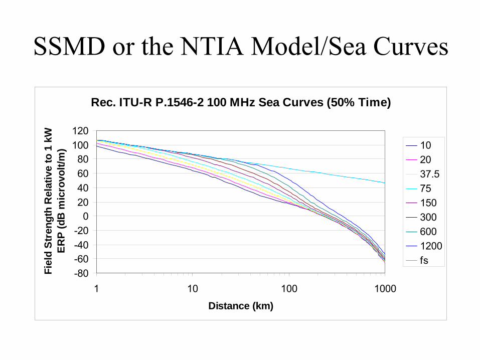
SSMD or the NTIA Model/Sea Curves
Rec. ITU-R P.1546-2 100 MHz Sea Curves (50% Time)
-80-60-40-20
020406080
100120
1 10 100 1000
Distance (km)
Fiel
d St
reng
th R
elat
ive
to 1
kW
ERP
(dB
mic
rovo
lt/m
) 102037.5751503006001200fs

SSMD or the NTIA Model/Sea Curves
Rec. ITU-R P.1546-2 600 MHz Sea Curves (50% Time)
-80-60-40-20
020406080
100120
1 10 100 1000
Distance (km)
Fiel
d St
reng
th R
elat
ive
to 1
kWER
P (d
B m
icro
volt/
m) 10
2037.5751503006001200fs
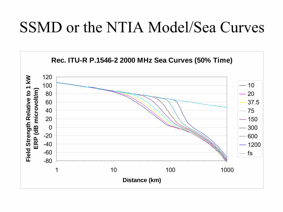
SSMD or the NTIA Model/Sea Curves
Rec. ITU-R P.1546-2 2000 MHz Sea Curves (50% Time)
-80-60-40-20
020406080
100120
1 10 100 1000
Distance (km)
Fiel
d St
reng
th R
elat
ive
to 1
kW
ERP
(dB
mic
rovo
lt/m
) 102037.5751503006001200fs

SSMD or the NTIA Model•
The Smooth Sphere Contribution, Ar
’–
Under line-of-sight conditions this should yield a direct ray-reflected ray model for a “smooth”
earth–
Under line-of-sight without first Fresnel zone clearance this should yield sub-
path diffraction
–
This latter method should blend smoothly into smooth sphere diffraction
( ) ( ))log(209.106)(
%50,,, 1,1546.'
ddE
fhdEdEA
fs
sPfsr
−=
−=

SSMD or the NTIA Model/Diffraction
Geometry for Deygout Construction

SSMD or the NTIA Model/Diffraction
•
Cascaded Knife Edge Diffraction (Deygout Construction)
( )
( )
( )
0
0
'
2
6)(
return
result to set the and ,...,1 ,0 with procedure srepeat thi
)78.0( 1.011.0log209.6)( where
04.010)()(1)(
,...,),max( and ,...,1),max(
find also then 78.0 if2
where2
path) los 0( ,...,1 ),max(
ddk
dn
rt
J
pd
jrit
p
ab
anbnba
e
nbann
nban
abn
pnp
LLA
Lnpflnh
J
dJJeJL
npflpjpi
ddhdh
addhh
dddhv
npfln
p
−=
==
−>⎟⎠⎞⎜
⎝⎛ −++−+=
+++⋅⎟⎟⎠
⎞⎜⎜⎝
⎛−+=
====
−>
+−+==
⇒<==
−
νννν
ννν
νννν
νλ
ννν
ν

SSMD or the NTIA Model•
The Weighted Combination of Smooth Sphere and Cascaded Knife Edge Diffraction, Comparison to Troposcatter and the Final Prediction
( ) ( ) ( )( )( ) ( )( )%50,,,,,,
,min
)2()(
,max ,8.01)(
101010,)(min
039.011factor weighting
1,1546.1,1546.50
50,'
50
'''
50
21
3
fhdEpfhdEAA
dEdEdAA
AwAwdA
addhedh
dadd
hhhhdhQ
Qw
lPlPp
tropofsdiff
rkdiff
e
lrltrte
d
eelrlt
grgt
eret
−+=
−=
⋅+⋅−=
⎟⎟⎠
⎞⎜⎜⎝
⎛ +−+=Δ⋅⎟⎟
⎠
⎞⎜⎜⎝
⎛−=Δ
⋅+++⎟
⎟⎠
⎞⎜⎜⎝
⎛
++
⋅⎟⎠⎞
⎜⎝⎛ Δ=
+=
−θθθ
θλ

Comparisons of the Path-Specific Models’
Features
•
Terrain (possibly Irregular Terrain) Diffraction Mechanisms
•
Line-of-Sight Mechanisms•
Troposcatter Mechanisms
•
Anomalous Propagation Mechanisms•
Land Use–Land Clutter/Site-Shielding Mechanisms
•
Building Entry Loss Mechanisms•
Radiometeorological Parameters and Time, Location (and Situation) Variabilities
•
Blending the Mechanisms (i.e., predicting enhancements at low time percentages)

Comparison of the Models’
Features•
Terrain Diffraction Mechanisms–
the Rec. ITU-R P.452, the Chinese and EBU Models each use the Deygout 3 knife-edge construction as found in Rec. ITU-R P.526
•
the EBU Model restricts the location of the subsidiary edges•
the Chinese Model uses smooth sphere diffraction for “flat”
paths•
Some differences in how the time variability is treated, Chinese
Model uses P.1546, while the others blend to reach the desired time percentage
–
the SSMD/NTIA Model uses the Deygout 3 knife-edge construction with the “smooth earth”
contribution removed plus smooth sphere diffraction from the P.1546 Sea Curves
•
median only until the Rec. ITU-R P.1546 land curves are factored in–
the Swiss Model advocates the Bullington Method•
median only–
the ITS’
ITM uses “double knife-edge”
plus smooth sphere diffraction attenuation plus an additional clutter correction, Afo , to account for obstructions between the radio horizons
•
median only, until the time, location and situation variabilities are factored in

Comparison of the Models’
Features (cont’d)
•
Line-of-Sight Mechanisms–
the ranges at which these mechanisms take place differ between the models
•
ITM appears to be much different from the Rec. ITU-R P.452 based models in this regard
–
All models use free space loss as the “dominant” mechanism with first Fresnel zone clearance
•
Rec. ITU-R P.452 includes multipath enhancements for time percentages less than 50%
–
Most models account for loss of first Fresnel zone clearance via sub-path diffraction
–
ITM includes the ground reflection contribution•
the other models do not explicitly do so, other than a nominal contribution in SSMD/NTIA

Comparison of the Models’
Features (cont’d)
•
Troposcatter Mechanisms–
These give rise to signal enhancements at (generally) small time percentages
–
The ITU-R P.452/Chinese/EBU Model is designed to blend smoothly with the other signal enhancement mechanisms
–
The ITM mechanism is designed to match with empirical and physical models of the expected phenomena.
–
The SSMD/NTIA uses the absolute prediction of the ITU- R P.452 Model to predict troposcatter losses

Comparison of the Models’
Features (cont’d)
•
Anomalous Propagation Mechanisms–
Explicitly treated through Rec. ITU-R P.452 (not including the Chinese Model) based models
–
Treated through the variabilities in ITM and P.1546 variability based models
•
Land-Use/Land-Clutter/Site-Shielding Losses–
each model’s formulation is different
–
Chinese and EBU’s Models for LU-LC losses have frequency dependence
•
Building Entry Loss–
A feature of the EBU Model only, but this could be adopted by the other models

Comparison of the Models’
Features (cont’d)
•
Radiometeorological Parameters and Time, Location and Situation Variabilities–
P.452, the Chinese and EBU models take global maps of radiometeorological parameters into account to assess effects of
time variability into account
–
ITM uses the radio climate to assess time variability, but requires user specification of the radio climate
–
all of the models take time variability into account•
each assumes that the time variability is normally distributed–
some models (P.452, Chinese and EBU) take the time percentage, p%, explicitly into account in the computation of all propagation mechanisms while others combine the variabilities after computation of an overall mean/median
•
Location and Situation Variabilities are an open question: only ITM considers situation variability

Comparison of the Models’
Features (cont’d)
•
Blending the Different Mechanisms–
ITM method: forces continuity at the “break points”, requires a continuously increasing attenuation with path distance
–
Rec. ITU-R P.452 method:•
blend via antilog-log combining process plus other mechanisms
( )⎟⎠⎞
⎜⎝⎛ ++
⋅= bA
bA naa
abA)(ln...ln 1
i.e.,