Path Integral Monte Carlo and the Worm Algorithm in the Spatial Continuum

Adrian Del Maestro∗

Department of Physics, University of Vermont, Burlington, VT 05405, USA(Dated: June 2, 2014)

The goal of these lecture notes will be to describe a stochastically exact quantum Monte Carlo method for computingthe expectation value of observables for systems of interacting particles in the spatial continuum described by aHamiltonian which conserves particle number. The latest version of the notes can always be found online at https://github.com/agdelma/pimc-notes while instructions on how to obtain, install and run our groups continuous spaceworm algorithm code are located at http://code.delmaestro.org.

I. EXPECTATION VALUES AND THE PARTITION FUNCTION

We begin with the general definition for the expectation value of some operator O in terms of a trace over config-urations

〈O〉 =1

ZTr Oe−βH (1)

where β = 1/kBT with kB the Boltzmann constant and the partition function Z is given by

Z = Tr e−βH = Tr ρ (2)

where

ρ ≡ e−βH (3)

is the density matrix. In order to compute the trace in Eq. (2) for a given system described by Hamiltonian H weneed to identify a set of convenient basis states |γ〉 that can be efficiently sampled allowing us to write the partitionfunction as the direct sum

Z =∑γ

〈γ|e−βH|γ〉

≈∑γ

W (γ) (4)

where W (γ) is a positive real weight corresponding to configuration state |γ〉. In the next section we will introducethe specific form of |γ〉 in terms of the spatial positions of interacting particles and describe a method for computingthe partition function as a sum of weights.

II. PATH INTEGRAL MONTE CARLO

The path-integral Monte Carlo method was first introduced by David Ceperley, and a comprehensive review canbe found in Ref. [1]. Here we will attempt to provide an introduction to the method with sufficient details to allowfor the creation of a simple code.

We are interested in a system of interacting particles described by the general many-body Hamiltonian:

H = T + V

= −N∑i=1

~2

2mi∇

2

i +

N∑i=1

Vi +∑i<j

Uij . (5)

It will be convenient to work in first quantized notation, where the N particles in the d-dimensional spatial continuumare located at positions ri with i = 1 . . . N . The first term in Eq. (5) corresponds to the kinetic energy T where mi

is the mass of the ith particle. The external potential energy V (ri) only depends on the position of a single particle,

2

while the two-body interaction potential U(ri− rj) is in general a function of the vector displacement between them.We will most often work with spherically symmetric interaction potentials such that U(ri−rj) = U(|ri−rj |) and we

will neglect all self-interactions: Uii = 0. A physical system of interest could include trapped ultra-cold atoms, whereV (ri) ∼ |ri|2 is a harmonic trapping potential and the particles interact via an induced dipole-dipole interactionU(ri − rj) ∼ |ri − rj |−3.

The most natural basis states |γ〉 are just a collection of the spatial locations of the N particles, where in the caseof identical particles, the labels are fictitious. We will employ the convenient short-hand notation

|R〉 ≡ |r1, · · · , rN 〉 (6)

where particle conservation enforces the normalization constraint∫DR |R〉〈R| = 1 (7)

with ∫DR ≡

N∏i=1

∫dri. (8)

In the first-quantized spatial position basis, the partition function can be written as a N × d dimensional integral

Z = Tr e−βH

=

∫dr1 · · ·

∫drN 〈r1, · · · , rN |e−βH|r1, · · · , rN 〉

≡∫DR〈R|e−βH|R〉. (9)

As terms like this will appear quite frequently, it will be useful to define the elements of the density matrix at inversetemperature β in the spatial basis

ρ(R,R′;β) ≡ 〈R|e−βH|R′〉 (10)

where all matrix elements are real and positive. We note that in the spatial continuum, the Hilbert space is uncountablyinfinite, as the particles can take on any position in Rd. This is an important observation that will guide the strategywe choose in the duration of these notes. Using the expression for ρ(R,R′;β) we can write the partition function:

Z =

∫DR ρ(R,R;β). (11)

As we have defined the potential operator V to be diagonal in the position basis, it would be extremely convenientif we could decompose the density matrix into a product of terms containing T and V. However, we know that[T , V] 6= 0 and thus

ρ = e−β(T +V)

6= e−βT e−βV . (12)

In fact, by employing the Baker-Campbell-Hausdorff formula we know:

eε(A+B) = eεAeεBe−ε2

2 [A,B] (13)

where ε ∈ C and thus

ρ = e−βT e−βV + O(β2). (14)

with the error diverging in the interesting (and quantum) low temperature limit β � 1. However, we may make the

rather self-evident observation that the Hamiltonian must commute with itself, [H, H] = 0 thus

ρ = e−βH

= e−β2 H−

β2 H

= e−β2 He−

β2 H. (15)

3

In the position basis, this corresponds to the elements of the density matrix satisfying a convolution relation

ρ(R,R′;β) = 〈R|e−βH|R′〉

= 〈R|e−β2 He−

β2 H|R′〉

=

∫DR′′ 〈R|e−

β2 H|R′′〉〈R′′|e−

β2 H|R′〉

=

∫DR′′ ρ

(R,R′′;

β

2

)ρ

(R′′,R′;

β

2

)(16)

where have employed the normalization condition in Eq. (7) and we note that the individual density matrices are ata higher effective temperature: β → β/2 ⇒ T → 2T . Now, returning to Eq. (11), we can employ this convolutionrelation M times where M ∈ Z� 1 to yield a new expression for the partition function

Z =

∫DR ρ(R,R;β)

=

∫DR0 · · ·

∫DRM−1 ρ

(R0,R1;

β

M

)· · · ρ

(RM−1,R0;

β

M

)(17)

where we have introduced the new notation

|Rα〉 ≡ |r1,α, · · · , rN,α〉. (18)

Until now, we have not specified the symmetry of the particles, but for the duration of these notes we will considersystems of identical bosons and thus we can write Eq. (17) in a more compact form:

Z =1

N !

∑P

M−1∏α=0

∫DRα ρ

(Rα,Rα+1;

β

M

)(19)

where the sum is over all permutations P of the fictitious particle labels i, and we require

|RM 〉 = P|R0〉 =∣∣rP(1),0, · · · rP(N),0

⟩(20)

to ensure the trace is non-zero.Upon closer examination of the individual terms in the product, we may notice:

〈Rα|e−β2 H|Rα+1〉 =

⟨Rα

∣∣∣∣U (−i~ βM)∣∣∣∣Rα+1

⟩(21)

where

U(t) ≡ e−itH/~ (22)

is the unitary time evolution operator of single particle quantum mechanics. Through the definition:

t = −i~τ (23)

where

τ ≡ β

M(24)

we may identify Eq. (19) as the partition function of a N particle system which evolves in an imaginary time direction.The configurations of our system now correspond to M discrete classical configurations corresponding to the positionsof the N particles: |r1,α, · · · , rN,α〉 where adjacent configurations in imaginary time at ατ and (α+1)τ are connectedvia an insertion of the short-imaginary-time propagator

ρ(Rα,Rα+1; τ) = 〈Rα|e−β2 H|Rα+1〉

= 〈Rα|U(−i~τ)|Rα+1〉.

This is simply a re-statement of the discrete Feynman path integral formulation of quantum statistical mechanics2,or equivalently the quantum-classical mapping, which says that a d-dimensional quantum system can be representedas a (d + 1)-dimensional classical system, where the extra (+1)th dimension is potentially subject to an additionalboundary condition.

4

imagin

ary

tim

e

space

2

0

3

4

5

6

7

spacer1,0 r2,0 r3,0 r4,0 r1,0 r2,0 r3,0 r4,0

r1,8 = r1,0 r2,8 = r2,0 r3,8 = r3,0 r4,8 = r4,0 r1,8 = r1,0 r3,8 = r2,0 r2,8 = r3,0 r4,8 = r4,0

(a) (b)

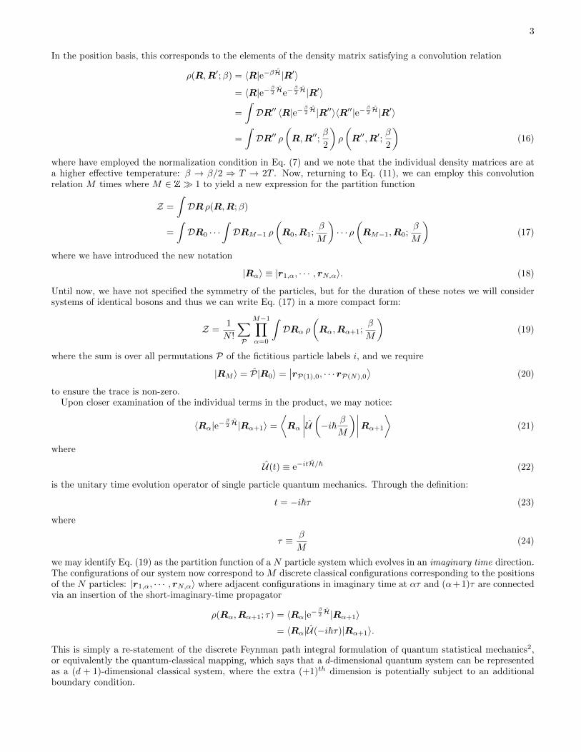
FIG. 1. A sample configuration N = 4 particles in d spatial dimensions (d = 1 here) where we have chosen M = 8 such thatτ = β/8. The actual spatial positions of the particles are identical in panels (a) and (b), however they differ by a reconnectionbetween imaginary times 2τ and 3τ corresponding to a permutation of the particle labels |R8〉a = |R0〉 = |r1,0, r2,0, r3,0, r4,0〉while |R8〉b = P|R0〉 = |r1,0, r3,0, r2,0, r4,0〉.

x-direction

r1,0

(a)

r1,2

r1,5

r1,7

r1,4

r1,1

r1,3

r1,6

y-direction

x-direction

(b)

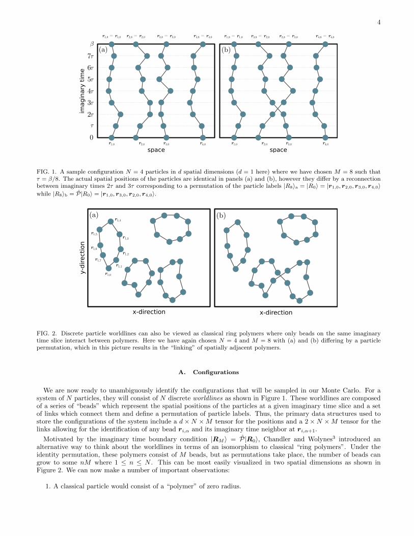
FIG. 2. Discrete particle worldlines can also be viewed as classical ring polymers where only beads on the same imaginarytime slice interact between polymers. Here we have again chosen N = 4 and M = 8 with (a) and (b) differing by a particlepermutation, which in this picture results in the “linking” of spatially adjacent polymers.

A. Configurations

We are now ready to unambiguously identify the configurations that will be sampled in our Monte Carlo. For asystem of N particles, they will consist of N discrete worldlines as shown in Figure 1. These worldlines are composedof a series of “beads” which represent the spatial positions of the particles at a given imaginary time slice and a setof links which connect them and define a permutation of particle labels. Thus, the primary data structures used tostore the configurations of the system include a d×N ×M tensor for the positions and a 2×N ×M tensor for thelinks allowing for the identification of any bead ri,α and its imaginary time neighbor at ri,α+1.

Motivated by the imaginary time boundary condition |RM 〉 = P|R0〉, Chandler and Wolynes3 introduced analternative way to think about the worldlines in terms of an isomorphism to classical “ring polymers”. Under theidentity permutation, these polymers consist of M beads, but as permutations take place, the number of beads cangrow to some nM where 1 ≤ n ≤ N . This can be most easily visualized in two spatial dimensions as shown inFigure 2. We can now make a number of important observations:

1. A classical particle would consist of a “polymer” of zero radius.

5

2. The spatial extent of a polymer is related to the thermal de Broglie wavelength λdB =√

2π~2/mkBT .

3. For a finite size system with periodic boundary conditions, worldlines can wind around the cell as the numberof beads per polymer grows via permutations which are more favorable at low temperatures. The width of thedistribution of integer winding numbers is related to the superfluid fraction.

B. Weights

Now that we have identified our configurations, in order to devise a sampling scheme we must return to the partitionfunction in Eq. (19) and attempt to compute the weights. Our construction thus far has been approximation free,and we have yet to utilize the fact that the new form of the partition function includes the elements of effective hightemperature density matrices in the limit where M � 1. Consider a single transition amplitude:

ρ(Rα,Rα+1; τ) = 〈Rα|e−τ(T+V )|Rα+1〉 (25)

where we can now ignore the fact that [T , V] 6= 0 at the cost of an error that grows as τ2. This is the PrimitiveApproximation and the error can be made arbitrarily small at a given temperature at the linear cost of increasing M .In practice, we can utilize various schemes to drastically improve the error by explicitly evaluating the commutator thatappears in Eq. (13) and we have chosen to employ a fourth order scheme called the generalized Suzuki factorization4.For the purposes of these lecture notes, the primitive approximation will be sufficient to illustrate all concepts andwe can write

ρ(Rα,Rα+1; τ) = 〈Rα|e−τ T e−τ V)|Rα+1〉+ O(τ2)

=

∫DR′ 〈Rα|e−τ T |R′〉〈R′|e−τ V)|Rα+1〉

=

∫DR′ 〈Rα|e−τ T |R′〉〈R′|Rα+1〉e−τV(Rα+1)

=

∫DR′ 〈Rα|e−τ T |R′〉δ(R′ −Rα+1)e−τV(Rα+1)

= 〈Rα|e−τ T |Rα+1〉e−τV(Rα+1) (26)

where we have inserted a complete set of states in line 2 and utilized the fact that the potential energy operatoris diagonal in imaginary time. We have introduced a slight abuse of the set notation R = {r1, · · · , rN} where, forexample, the Dirac delta function is understood to mean

δ(R−R′) ≡N∏i=1

δ(ri − r′i) (27)

and

V(R) ≡N∑i=1

V (ri) +1

2

∑i,j

U(ri − rj). (28)

Since the kinetic energy operator T is clearly not diagonal in the spatial position basis, in order to compute the firstterm in Eq. (26) we can write the position eigenstate in terms of free particle plane waves

|R〉 = |r1, · · · , rN 〉

=

N∏i=1

∫dki

(2π)deiki·ri |k1, · · · ,kN 〉. (29)

Defining

λ ≡ ~2

2m(30)

6

we can write

〈R|e−τ T |R′〉 =

N∏i=1

∫dki

(2π)d

∫dk′i

(2π)de−iki·rieik

′i·r

′i

⟨k1, · · · ,kN

∣∣∣e−τλ∑Nj=1 ∇2

j

∣∣∣k′1, · · · ,k′N⟩=

N∏i=1

∫dki

(2π)d

∫dk′i

(2π)de−λτ |k

′i|

2−iki·ri+ik′i·r

′i⟨k1, · · · ,kN |k′1, · · · ,k

′N

⟩=

N∏i=1

∫dki

(2π)d

∫dk′i

(2π)de−λτ |k

′i|

2−iki·ri+ik′i·r

′i(2π)dδ(ki − k′i)

=

N∏i=1

∫dki

(2π)de−λτ |ki|

2+iki·(r′i−ri)

= (4πλτ)−Nd/2exp

[− 1

4λτ

N∑i=1

|ri − r′i|2]

(31)

which is just the free particle propagator that can be written in our set notation as

ρ0(R,R′; τ) =⟨R∣∣∣e−τ T ∣∣∣R′⟩

= (4πλτ)−Nd/2e−1

4λτ |R−R′|2 . (32)

We may now insert our complete expression for the primitive imaginary time propagator

ρ(Rα,Rα+1; τ) = ρ0(Rα,Rα+1; τ)e−τV(Rα) (33)

into the partition function in Eq. (19) to find

Z = (4πλτ)−NMd/2 1

N !

∑P

M−1∏α=0

∫DRα e−

14λτ |Rα−Rα+1|2−τV(Rα)

= (4πλτ)−NMd/2 1

N !

∑P

M−1∏α=0

N∏i=1

∫dri,α exp

−M∑α=0

N∑i=1

|ri,α+1 − ri,α|2

4λτ+ τV (ri,α) +

τ

2

N∑j=1

U(ri,α − rj,α)

.

(34)

Because of the product of M copies of the primitive propagator, the finite Trotter error we make in the partitionfunction is O(τ). This partition function is then just a “path” integral over all possible configurations and permutationsof particle worldlines where the weight of each configuration is just the exponentiated effective action.

C. Updates

In order to sample configurations we must devise a series of updates that can be proposed and accepted or rejectedbased on their weights. We are aided by the fact that it is possible to exactly sample the free density matrixρ0(R,R′; τ) since it is just a product of Gaussians. This will allow us to sample the kinetic part of the action inthe ensemble and only consider the potential action in the weights. We will outline two types of simple updates,center-of-mass and staging moves, and briefly discuss a third permutation move that will present us with a difficultchallenge.

1. Center of Mass

A center-of-mass update involves the spatial translation of an entire worldline, leaving the kinetic part of the actionunchanged. It is shown schematically in Figure 3 and proceeds as follows:

1. Choose a random integer i ∈ [0, N − 1] fixing worldline i with beads located at ri,α.

7

imagin

ary

tim

e

0space

center of

mass

space

FIG. 3. A center of mass Monte Carlo update, which translates the entire worldline i by a vector displacement ∆ withoutmodifying the connections between beads.

2. Generate uniformly distributed random numbers, ∆a, where a = 1, . . . , d on (−δ/2, δ/2) where δ is a smallnumber that can be modified to optimize the acceptance rate. Construct the vector ∆ = (∆1, . . . ,∆d).

3. Translate the entire worldline by ∆ to obtain a new set of coordinates r′i,α where r′i,α = ri,α + D for α =0, . . . ,M − 1.

4. Accept the update with probability

Pcom = min{

1, e−τ [V(r′i)−V(ri)]

}(35)

where

V(ri) ≡M−1∑α=0

V (ri,α) +1

2

N∑j=1

U(ri,α − rj,α)

. (36)

2. Staging

A staging update5 generates a new section of path between two fixed beads at time slices α and α + m wherem < M is an algorithmic parameter that can be tuned to optimize the acceptance rate. It utilizes the fact that thefree particle density matrix in Eq. (32) is Gaussian and thus obeys a convolution relation. The problem is as follows:given two known spatial positions (beads) on worldline i, say ri,α and ri,α+m, how do we exactly sample the productof free particle density matrices:

ρ0(ri,α, ri,α+1; τ) · · · ρ0(ri,α+m−1, ri,α+m; τ) ? (37)

The solution comes by choosing a single term in this product and constructing the probability distribution for prop-agation to that position, constrained by the endpoints. Let us drop the worldline index i for brevity:

π0(rγ |rα, rα+m) = ρ0(rα, rγ ; (γ − α)τ)ρ0(rγ , rα+m; (α+m− γ)τ)

∝ exp

[− |rγ − rα|2

4λ(γ − α)τ

]exp

[− |rα+m − rγ |2

4λ(α+m− γ)τ

]∝ exp

[−|rγ − rγ |2

2σ2

](38)

8

imagin

ary

tim

e

0space

staging

space

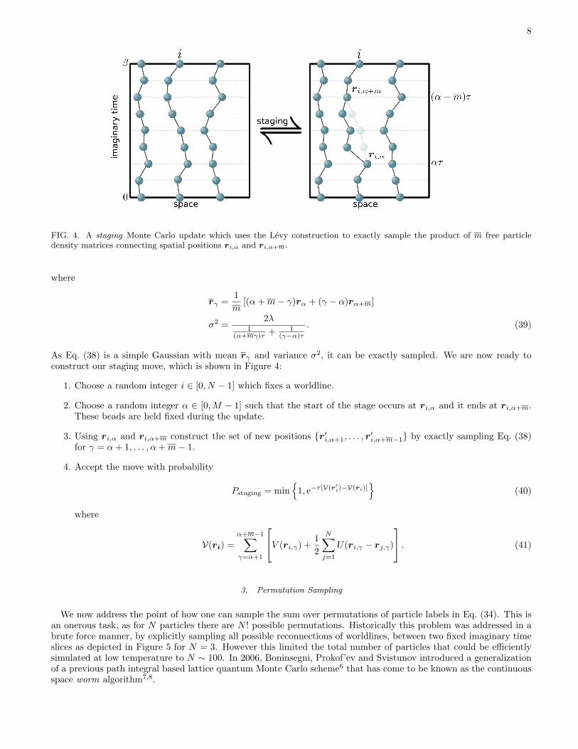
FIG. 4. A staging Monte Carlo update which uses the Levy construction to exactly sample the product of m free particledensity matrices connecting spatial positions ri,α and ri,α+m.

where

rγ =1

m[(α+m− γ)rα + (γ − α)rα+m]

σ2 =2λ

1(α+mγ)τ + 1

(γ−α)τ

. (39)

As Eq. (38) is a simple Gaussian with mean rγ and variance σ2, it can be exactly sampled. We are now ready toconstruct our staging move, which is shown in Figure 4:

1. Choose a random integer i ∈ [0, N − 1] which fixes a worldline.

2. Choose a random integer α ∈ [0,M − 1] such that the start of the stage occurs at ri,α and it ends at ri,α+m.These beads are held fixed during the update.

3. Using ri,α and ri,α+m construct the set of new positions {r′i,α+1, . . . , r′i,α+m−1} by exactly sampling Eq. (38)

for γ = α+ 1, . . . , α+m− 1.

4. Accept the move with probability

Pstaging = min{

1, e−τ [V(r′i)−V(ri)]

}(40)

where

V(ri) =

α+m−1∑γ=α+1

V (ri,γ) +1

2

N∑j=1

U(ri,γ − rj,γ)

. (41)

3. Permutation Sampling

We now address the point of how one can sample the sum over permutations of particle labels in Eq. (34). This isan onerous task, as for N particles there are N ! possible permutations. Historically this problem was addressed in abrute force manner, by explicitly sampling all possible reconnections of worldlines, between two fixed imaginary timeslices as depicted in Figure 5 for N = 3. However this limited the total number of particles that could be efficientlysimulated at low temperature to N ∼ 100. In 2006, Boninsegni, Prokof’ev and Svistunov introduced a generalizationof a previous path integral based lattice quantum Monte Carlo scheme6 that has come to be known as the continuousspace worm algorithm7,8.

9

imag

inary

tim

e

0space space space

imag

inary

tim

e

0

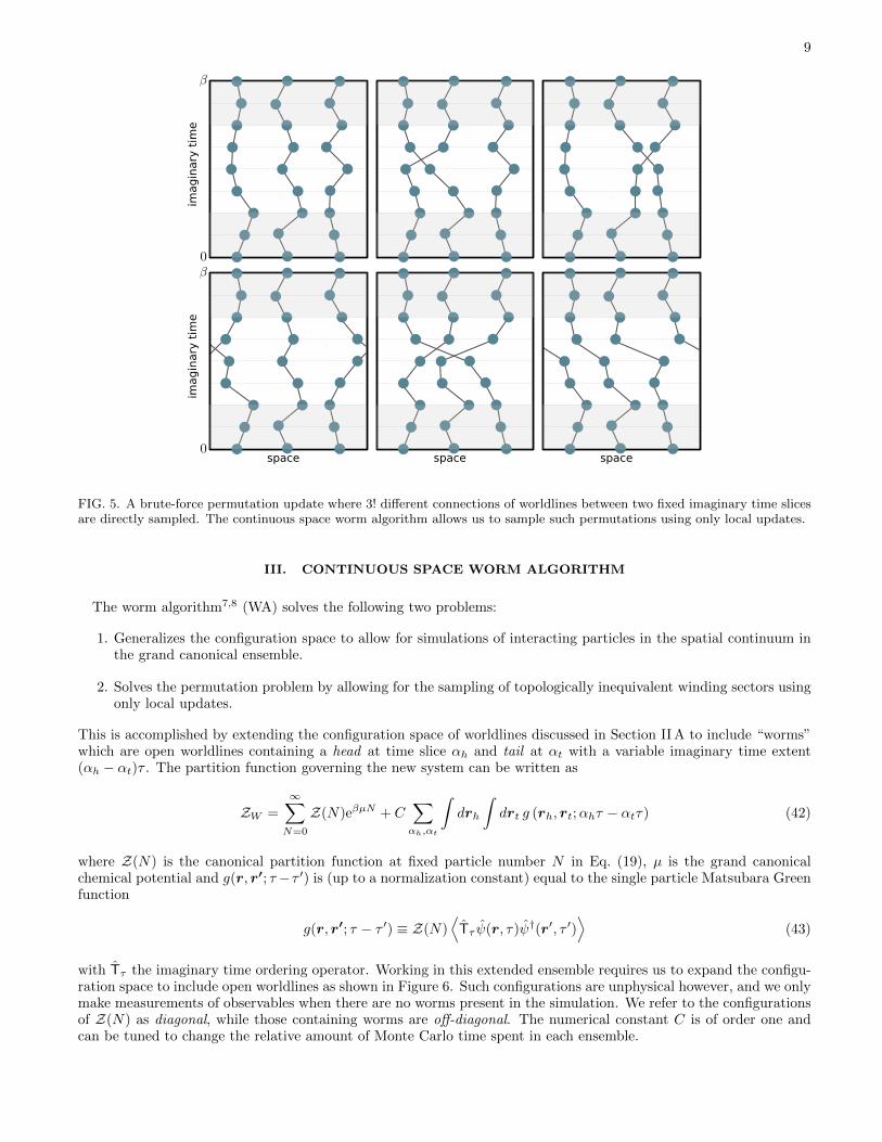
FIG. 5. A brute-force permutation update where 3! different connections of worldlines between two fixed imaginary time slicesare directly sampled. The continuous space worm algorithm allows us to sample such permutations using only local updates.

III. CONTINUOUS SPACE WORM ALGORITHM

The worm algorithm7,8 (WA) solves the following two problems:

1. Generalizes the configuration space to allow for simulations of interacting particles in the spatial continuum inthe grand canonical ensemble.

2. Solves the permutation problem by allowing for the sampling of topologically inequivalent winding sectors usingonly local updates.

This is accomplished by extending the configuration space of worldlines discussed in Section II A to include “worms”which are open worldlines containing a head at time slice αh and tail at αt with a variable imaginary time extent(αh − αt)τ . The partition function governing the new system can be written as

ZW =

∞∑N=0

Z(N)eβµN + C∑αh,αt

∫drh

∫drt g (rh, rt;αhτ − αtτ) (42)

where Z(N) is the canonical partition function at fixed particle number N in Eq. (19), µ is the grand canonicalchemical potential and g(r, r′; τ−τ ′) is (up to a normalization constant) equal to the single particle Matsubara Greenfunction

g(r, r′; τ − τ ′) ≡ Z(N)⟨Tτ ψ(r, τ)ψ†(r′, τ ′)

⟩(43)

with Tτ the imaginary time ordering operator. Working in this extended ensemble requires us to expand the configu-ration space to include open worldlines as shown in Figure 6. Such configurations are unphysical however, and we onlymake measurements of observables when there are no worms present in the simulation. We refer to the configurationsof Z(N) as diagonal, while those containing worms are off-diagonal. The numerical constant C is of order one andcan be tuned to change the relative amount of Monte Carlo time spent in each ensemble.

10

imagin

ary

tim

e

space0

head

tail

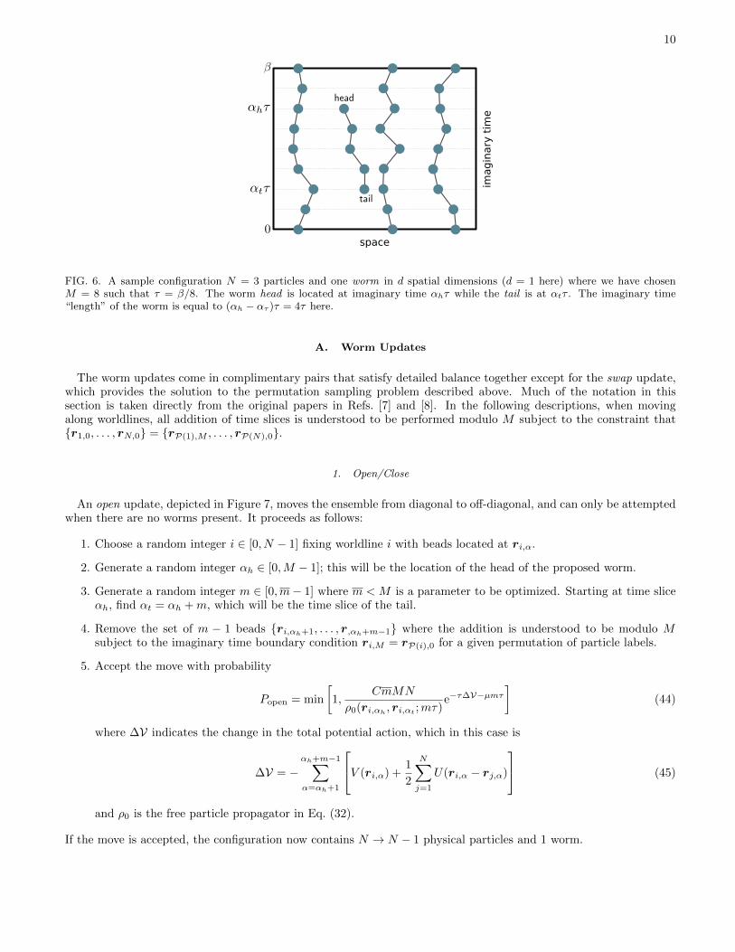
FIG. 6. A sample configuration N = 3 particles and one worm in d spatial dimensions (d = 1 here) where we have chosenM = 8 such that τ = β/8. The worm head is located at imaginary time αhτ while the tail is at αtτ . The imaginary time“length” of the worm is equal to (αh − ατ )τ = 4τ here.

A. Worm Updates

The worm updates come in complimentary pairs that satisfy detailed balance together except for the swap update,which provides the solution to the permutation sampling problem described above. Much of the notation in thissection is taken directly from the original papers in Refs. [7] and [8]. In the following descriptions, when movingalong worldlines, all addition of time slices is understood to be performed modulo M subject to the constraint that{r1,0, . . . , rN,0} = {rP(1),M , . . . , rP(N),0}.

1. Open/Close

An open update, depicted in Figure 7, moves the ensemble from diagonal to off-diagonal, and can only be attemptedwhen there are no worms present. It proceeds as follows:

1. Choose a random integer i ∈ [0, N − 1] fixing worldline i with beads located at ri,α.

2. Generate a random integer αh ∈ [0,M − 1]; this will be the location of the head of the proposed worm.

3. Generate a random integer m ∈ [0,m− 1] where m < M is a parameter to be optimized. Starting at time sliceαh, find αt = αh +m, which will be the time slice of the tail.

4. Remove the set of m − 1 beads {ri,αh+1, . . . , r,αh+m−1} where the addition is understood to be modulo Msubject to the imaginary time boundary condition ri,M = rP(i),0 for a given permutation of particle labels.

5. Accept the move with probability

Popen = min

[1,

CmMN

ρ0(ri,αh , ri,αt ;mτ)e−τ∆V−µmτ

](44)

where ∆V indicates the change in the total potential action, which in this case is

∆V = −αh+m−1∑α=αh+1

V (ri,α) +1

2

N∑j=1

U(ri,α − rj,α)

(45)

and ρ0 is the free particle propagator in Eq. (32).

If the move is accepted, the configuration now contains N → N − 1 physical particles and 1 worm.

11

imagin

ary

tim

e

0space

head

tail

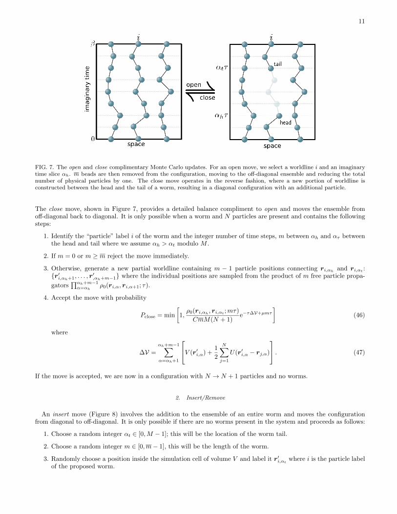
FIG. 7. The open and close complimentary Monte Carlo updates. For an open move, we select a worldline i and an imaginarytime slice αh. m beads are then removed from the configuration, moving to the off-diagonal ensemble and reducing the totalnumber of physical particles by one. The close move operates in the reverse fashion, where a new portion of worldline isconstructed between the head and the tail of a worm, resulting in a diagonal configuration with an additional particle.

The close move, shown in Figure 7, provides a detailed balance compliment to open and moves the ensemble fromoff-diagonal back to diagonal. It is only possible when a worm and N particles are present and contains the followingsteps:

1. Identify the “particle” label i of the worm and the integer number of time steps, m between αh and ατ betweenthe head and tail where we assume αh > αt modulo M .

2. If m = 0 or m ≥ m reject the move immediately.

3. Otherwise, generate a new partial worldline containing m − 1 particle positions connecting ri,αh and ri,αt :{r′i,αh+1, . . . , r

′,αh+m−1} where the individual positions are sampled from the product of m free particle propa-

gators∏αh+m−1α=αh

ρ0(ri,α, ri,α+1; τ).

4. Accept the move with probability

Pclose = min

[1,ρ0(ri,αh , ri,αt ;mτ)

CmM(N + 1)e−τ∆V+µmτ

](46)

where

∆V =

αh+m−1∑α=αh+1

V (r′i,α) +1

2

N∑j=1

U(r′i,α − rj,α)

. (47)

If the move is accepted, we are now in a configuration with N → N + 1 particles and no worms.

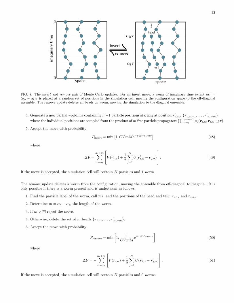
2. Insert/Remove

An insert move (Figure 8) involves the addition to the ensemble of an entire worm and moves the configurationfrom diagonal to off-diagonal. It is only possible if there are no worms present in the system and proceeds as follows:

1. Choose a random integer αt ∈ [0,M − 1]; this will be the location of the worm tail.

2. Choose a random integer m ∈ [0,m− 1], this will be the length of the worm.

3. Randomly choose a position inside the simulation cell of volume V and label it r′i,αt where i is the particle labelof the proposed worm.

12

imag

inary

tim

e

0space

head

tail

space

insert

remove

i

FIG. 8. The insert and remove pair of Monte Carlo updates. For an insert move, a worm of imaginary time extent mτ =(αh − αt)τ is placed at a random set of positions in the simulation cell, moving the configuration space to the off-diagonalensemble. The remove update deletes all beads on worm, moving the simulation to the diagonal ensemble.

4. Generate a new partial worldline containingm−1 particle positions starting at position r′i,αt : {r′i,αt+1, . . . , r

′,αt+m}

where the individual positions are sampled from the product ofm free particle propagators∏αt+m−1α=αt

ρ0(ri,α, ri,α+1; τ).

5. Accept the move with probability

Pinsert = min[1, CV mMe−τ∆V+µmτ

](48)

where

∆V =

αt+m∑α=αt

V (r′i,α) +1

2

N∑j=1

U(r′i,α − rj,α)

. (49)

If the move is accepted, the simulation cell will contain N particles and 1 worm.

The remove update deletes a worm from the configuration, moving the ensemble from off-diagonal to diagonal. It isonly possible if there is a worm present and is undertaken as follows:

1. Find the particle label of the worm, call it i, and the positions of the head and tail: ri,αh and ri,αh .

2. Determine m = αh − αt, the length of the worm.

3. If m > m reject the move.

4. Otherwise, delete the set of m beads {ri,αt , . . . , r′,αt+m}.

5. Accept the move with probability

Premove = min

[1,

1

CVmMe−τ∆V−µmτ

](50)

where

∆V = −αt+m∑α=αt

V (ri,α) +1

2

N∑j=1

U(ri,α − rj,α)

. (51)

If the move is accepted, the simulation cell will contain N particles and 0 worms.

13

imag

inary

tim

e

0space

advance

recede

0space

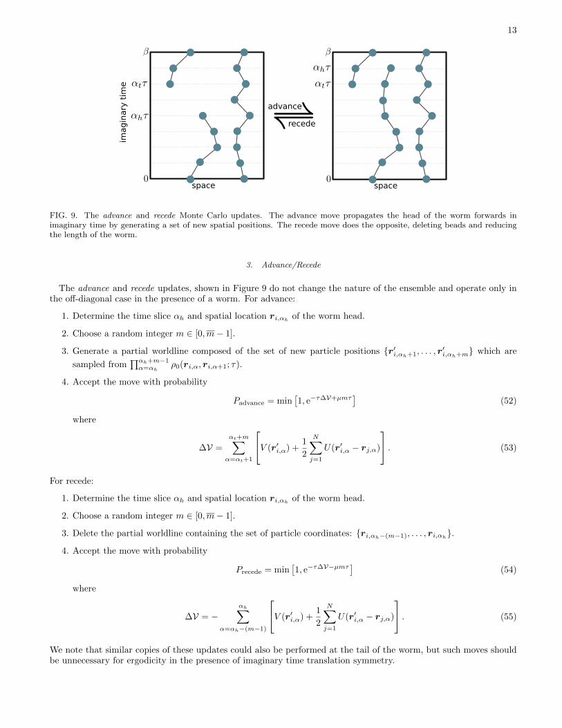
FIG. 9. The advance and recede Monte Carlo updates. The advance move propagates the head of the worm forwards inimaginary time by generating a set of new spatial positions. The recede move does the opposite, deleting beads and reducingthe length of the worm.

3. Advance/Recede

The advance and recede updates, shown in Figure 9 do not change the nature of the ensemble and operate only inthe off-diagonal case in the presence of a worm. For advance:

1. Determine the time slice αh and spatial location ri,αh of the worm head.

2. Choose a random integer m ∈ [0,m− 1].

3. Generate a partial worldline composed of the set of new particle positions {r′i,αh+1, . . . , r′i,αh+m} which are

sampled from∏αh+m−1α=αh

ρ0(ri,α, ri,α+1; τ).

4. Accept the move with probability

Padvance = min[1, e−τ∆V+µmτ

](52)

where

∆V =

αt+m∑α=αt+1

V (r′i,α) +1

2

N∑j=1

U(r′i,α − rj,α)

. (53)

For recede:

1. Determine the time slice αh and spatial location ri,αh of the worm head.

2. Choose a random integer m ∈ [0,m− 1].

3. Delete the partial worldline containing the set of particle coordinates: {ri,αh−(m−1), . . . , ri,αh}.

4. Accept the move with probability

Precede = min[1, e−τ∆V−µmτ ] (54)

where

∆V = −αh∑

α=αh−(m−1)

V (r′i,α) +1

2

N∑j=1

U(r′i,α − rj,α)

. (55)

We note that similar copies of these updates could also be performed at the tail of the worm, but such moves shouldbe unnecessary for ergodicity in the presence of imaginary time translation symmetry.

14

imagin

ary

tim

e

0space

swap

FIG. 10. The swap Monte Carlo update, which does not change the nature of the ensemble, but allows for the sampling ofdifferent topological sectors. A new partial worldline is generated between the head of the worm and a neighboring particleworldline position at an advanced time slice. The original portion of the particle worldline is then erased, “swapping” the headof the worm and increasing the imaginary time extent of the worm.

4. Swap

The swap update, shown in Figure 10 is behind the huge speedup inherent in the worm algorithm, as it allows usto sample different topological winding sectors (permutations) using only local updates. It does not, therefore, sufferfrom the horrendous N ! scaling of brute-force permutation sampling. It only operates on off-diagonal configurations,in the presence of a worm, and does not change the ensemble. It provides a method by which a single worm grows bynM time slices where 1 ≤ n ≤ N by “swapping” its head with a proximate unbroken particle worldline. To performa swap move:

1. Determine the time slice αh and spatial location ri,αh of the worm head.

2. Advance to the time slice of the pivot bead αp = αh + m where the addition is modulo M and find the set ofall beads `p ≡ {rk,αp} such that |ri,αh − rk,αp | < R where R ∈ R is a simulation parameter to be optimized.

3. Use tower sampling to select a single bead rj,αp ∈ {rk,αp} from the list with probability

Pp =1

Σpρ0(ri,αh , rj,αp ;mτ) (56)

where the normalization factor is

Σp =∑r∈`p

ρ0(ri,αh , r;mτ). (57)

4. Recede m time steps along worldline j from αp to identify the swap bead at αs = αh = αp −m: rj,αs . If thetail of the worm, ri,αt , is encountered during this process, immediately reject the move.

5. If |rj,αp − rj,αs | ≥ R reject the move.

6. Otherwise, create a second list `s ≡ {rk,αs} such that |rj,αs − rk,αp | < R and form the sum

Σs =∑r∈`s

ρ0(rj,αp , r;mτ). (58)

7. Delete the set of m− 1 beads {rj,αs+1, . . . , rj,αs+m−1}.

8. Construct a new partial worldline containing the set of particle positions {r′i,αh+1, . . . r′i,αh+m−1} connecting

ri,αh and rj,αp sampled from the product of m free particle propagators∏αh+m−1α=αh

ρ0(ri,α, ri,α+1; τ) whereri,αh+m = rj,αp .

15

9. The head of the worm is now located at rj,αs and its length has increased by the number of beads contained inthe particle that was labeled by j.

10. Accept the move with probability

Pswap = min

[1,

ΣpΣs

e−τ∆V]

(59)

where

∆V =

αh+m−1∑α=αh+1

{V (r′i,α)− V (rj,α) +

1

2

N∑k=1

[U(r′i,α − rk,α)− U(rj,α − rk,α)

]}. (60)

∗ Adrian.DelMaestro@uvm.edu1 D. M. Ceperley, Review Modern Physics 67, 279 (1995).2 R. Feynman and A. Hibbs, Quantum mechanics and path integrals, International series in pure and applied physics (McGraw-

Hill, 1965).3 D. Chandler and P. G. Wolynes, The Journal of Chemical Physics 74, 4078 (1981).4 S. Jang, S. Jang, and G. A. Voth, The Journal of Chemical Physics 115, 7832 (2001).5 M. Sprik, M. Klein, and D. Chandler, Physical Review B 31, 4234 (1985).6 N. Prokof’ev, Svistunov, B.V., and I. Tupitsyn, Physics Letters A 238, 253 (1998).7 M. Boninsegni, N. Prokof’ev, and B. Svistunov, Physical Review Letters 96, 070601 (2006).8 M. Boninsegni, N. V. Prokof’ev, and B. V. Svistunov, Physical Review E 74, 036701 (2006).