Path-Following Control for Coordinated Turn Aircraft...

Path-Following Control for Coordinated Turn

Aircraft Maneuvers

David Cabecinhas∗ and Carlos Silvestre† and Paulo Rosa‡ and Rita Cunha§

Instituto Superior Tecnico, Institute for Systems and Robotics, 1049-001 Lisbon, Portugal

This paper addresses the path-following problem of steering an autonomous airplanealong a predefined 3-D path, while performing a coordinated turn maneuver. The presentedsolution relies on the definition of a path-dependent error space to express the dynamicmodel of the vehicle, and of an output tracking error that guarantees both path-followingand coordinated turn compliance. For controller design purposes, the error dynamics areapproximated by a polytopic Linear Parameter Varying (LPV) system representation withpiecewise affine dependency on the parameters. The synthesis problem is stated as anH2 minimization problem with pole placement contraints, and solved using Linear MatrixInequalities (LMIs). The nonlinear controller is implemented within the scope of gain-scheduling control theory, using the D-methodology. The performance of the designedcontroller is assessed in simulation, using the full nonlinear model of a small scale airplane.

I. Introduction

In recent years, the advent of enabling technology in sensing, computation, and communications hasempowered Unmanned Aerial Vehicles (UAVs) to become cost-effective, reliable, and safe alternatives toconventional piloted aircraft in a wide variety of applications. For example, in forest fire surveillance, asmall unmanned autonomous aircraft equipped with a camera and other sensing devices can be used toautomatically detect fires and alert the nearest fire department. Other types of missions, where UAVsalready play a key role, include surveillance and reconnaissance operations. These assignments are typicallyconducted in hostile and unexplored territory, where the risk of losing the aircraft is high. With UAVs, thesemissions can be accomplished without endangering human lives. Autonomous vehicles have great potentialto perform high precision and repetitive tasks, since a whole new range of sensing devices can provide themwith information that is not perceptible by a pilot. With this added information, autonomous flight controlsystems can be designed to provide enhanced performance and efficiency.

Several different approaches to the problem of flight control for autonomous aircraft can be found inthe literature. For example, in References 1 and 2, nonlinear control strategies are used to address thetrajectory-tracking problem, whereas Shue et al.3 present a mixed H2/H∞ gain scheduling technique foraircraft control. A robust control solution for coordinated turn maneuvers is proposed in Reference 4.

This paper addresses the problem of aircraft control for coordinated turn maneuvers, using a path-following approach. By lifting the strict temporal restrictions that are dictated by a time-parameterizedreference, the path-following approach provides an alternative to trajectory-tracking that typically resultsin smoother convergence to the path and less demand on the control effort. The coordinated turn maneuverimproves the aircraft’s flying qualities and performance, by constraining the vehicle’s orientation to be suchthat there is no component of aerodynamic force along the y-axis of a body-fixed coordinate frame.5 In thispaper, the path-following problem is addressed along the lines of the work reported in References 6–8. Itrelies on applying a nonlinear transformation to aircraft dynamic model to obtain a conveniently definederror model. The resulting error vector comprises velocity errors, orientation errors, and the distance to the

∗PhD Student, Department of Electrical Engineering and Computer Science (DEEC), Av. Rovisco Pais 1;[email protected].

†Assistant Professor, DEEC, Av. Rovisco Pais 1; [email protected]. Member AIAA.‡PhD Student, DEEC, Av. Rovisco Pais 1; [email protected].§PhD Student, DEEC, Av. Rovisco Pais 1; [email protected].

1 of 19

American Institute of Aeronautics and Astronautics

AIAA Guidance, Navigation and Control Conference and Exhibit20 - 23 August 2007, Hilton Head, South Carolina

AIAA 2007-6656

Copyright © 2007 by the American Institute of Aeronautics and Astronautics, Inc. All rights reserved.

path, defined as the distance between the vehicle’s position and its orthogonal projection on the path. Inaddition, an output tracking error to be driven to zero at steady-state is defined, which explicitly includesthe coordinate turn constraint.

Having an accurate mathematical model of the airplane is an essential prerequisite for control system de-sign. In this paper, we present SimAirDyn - an airplane dynamic model implemented in MATLAB/Simulink,which is specially suited for controller design. The most significant effects, which determine the aircraft’sdynamic behavior and whose modeling requires special attention, are specified by the dimensionless aero-dynamic force and torque coefficients. Typically, these coefficients are experimentally obtained in a windtunnel. However, there are software alternatives to these tests, based on geometric models of the aircraft,which provide reasonable approximations for the coefficients with significant cost reduction. The latterapproach was adopted to build the referred simulation model.

Airplanes are complex nonlinear systems whose dynamic behavior changes significantly as a function ofthe dynamic pressure, and angles of attack and side-slip. Thus, it is insufficient, for purposes of controlsystem design, to represent them by simple Linear Time Invariant (LTI) models. Linear Parameter Varying(LPV) models represent nowadays a compromise between the global accuracy of nonlinear models and thestraightforward controller synthesis techniques available for LTI representations. Partitioning the flightenvelope into smaller regions, according to the relevant flight regime, simpler polytopic LPV models can beobtained, which are still accurate enough to capture the essential behavior of the aircraft and simultaneouslyprovide the working ground for the control design phase.

The methodology used for performance analysis and controller synthesis builds on results described inReferences 9–11, which cast these problems into a Linear Matrix Inequality (LMI) framework. LMIs aresteadily becoming a standard tool for advanced control system design, since both LMI feasibility and LMI-constrained optimization problems constitute convex optimization problems, for which efficient numericalsolvers are available. In this paper, we synthesize a continuous-time state feedback H2 controller subjectto pole placement constraints for each of the operating regions, and implement a nonlinear gain-schedulingcontroller based on the D-methodology.12

The paper is organized as follows. Section II presents the standard rigid-body dynamic model, which isused to describe the aircraft. We also describe the derivation of the aircraft nonlinear dynamic model andanalyze the natural modes obtained for the linearized model. Section III introduces the path-dependent errorspace and presents a derivation of the error dynamics. In Section IV, we describe the methodology used tocompute H2 controllers for polytopic LPV systems. The controller implementation using gain-scheduling andthe D-methodology is also discussed. Finally, in Section V, we present simulation results for the closed-loopnonlinear aircraft model, under the presence of wind disturbances.

II. Aircraft Dynamic Model

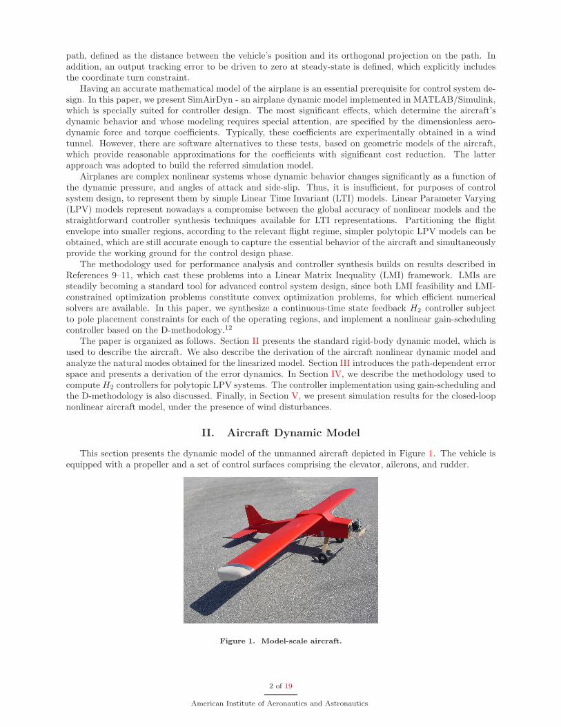
This section presents the dynamic model of the unmanned aircraft depicted in Figure 1. The vehicle isequipped with a propeller and a set of control surfaces comprising the elevator, ailerons, and rudder.

Figure 1. Model-scale aircraft.

2 of 19


The aircraft is modeled as a 6 degrees of freedom rigid-body, moving with respect to the inertial frame{I}, and whose equations of motion are expressed in the body frame {B} attached to the vehicle’s centerof mass. Let (IpB,

I

BR) ∈ SE(3) , R

3 × SO(3) denote the configuration of {B} with respect to {I}and λB = [φB θB ψB]

T, θB ∈ ]−π/2, π/2[, φB, ψB ∈ R denote the Z-Y-X Euler angles, representing the

orientation of {B} relative to {I}. The rotation matrix I

BR and the Euler angles λB satisfy

I

BR = RZ(ψB)RY (θB)RX(φB) ⇔ λB = arg( I

BR) ⇔

θB = atan2(−r31,√

r211 + r221)

φB = atan2(r32, r33)

ψB = atan2(r21, r11)

, (1)

where atan2(., .) denotes the four quadrant arctangent function and RZ(.), RY (.), and RX(.) denote rotationmatrices about the Z, Y , and X axes, respectively.

Consider also the linear and angular body velocities, vB = [u v w]T and ωB = [p q r]T ∈ R3, given

respectively by vB = B

IR IpB and ωB = B

IR IωB, where IωB ∈ R

3 denotes the angular velocity of {B}with respect to {I} expressed in {I}. According to this notation, the standard equations for the vehicle’skinematics13 can be written as

{

I pB = I

BRvB

λB = Q(φB , θB)ωB

, (2)

where

Q(φB, θB)=

1 sinφB tan θB cosφB tan θB

0 cosφB − sinφB

0 sinφB/cos θB cosφB/cos θB

, (3)

and the derivative of I

BR is given by I

BR = I

BRS(ωB), where S(x) ∈ R

3×3 is a skew symmetric matrix suchthat S(x) y = x× y, for all x, y ∈ R

3. Using the Newton-Euler equations, the dynamic model of the vehiclecan be written as

{

mvB + S(ωB)mvB = faero(vB ,ωB,u,w) + m B

IR [0 0 g]T

IωB + S(ωB)IωB = naero(vB ,ωB,u,w), (4)

where m ∈ R+ and I ∈ R

3×3 denote the aircraft’s mass and moment of inertia, respectively; g denotesthe gravitational acceleration; and faero, naero : (R3,R3,Rnu ,Rnw) → R

3 represent the external forces andmoments acting on the body, which are in general functions of the body velocities vB and ωB, controlinputs u ∈ R

5, and wind disturbances w ∈ R3. The control vector u = [T, δe, δac, δad, δr]

T comprisesthe propeller generated thrust δt and the surface deflections for the elevator δe, aileron common mode δac,aileron differential mode δad, and rudder δr.

The complete dynamic model of the aircraft can be written as

vB = f (vB, ωB , u, w) + fg (φB , θB)

ωB = n (vB , ωB, u, w)IpB = I

BRvB

λB = Q(φB , θB)ωB

, (5)

where

f = m−1faero − S(ωB)vB ,

n = I−1naero − I−1S(ωB)IωB,

fg = B

IR[0 0 g]T = RX(φB)TRY (θB)T [0 0 g]T

A. SimAirDyn Dynamic Model

SimAirDyn is an aircraft dynamic model designed for effective control system design and flight envelopeexpansion. The aircraft’s dynamics can be described using a six degree of freedom rigid body dynamicmodel (such as the one presented in (5)), which is driven by forces and moments that explicitly include theeffects of the propeller, fuselage, wings, and gravity.14–16 The remaining components, namely the landing

3 of 19


gear and the antennas, which have a smaller impact on the overall behavior of the aircraft dynamic model,are not included in the simulator and will naturally be treated as disturbances by the control system.

The aircraft nonlinear simulation model SimAirDyn was tuned to adequately capture the essential behav-ior of the actual vehicle for a large operational flight envelope.15, 16 The most important model parametersare the dimensionless aerodynamic force and torque coefficients, which can be obtained from a Taylor seriesexpansion of the force and torque functions about selected operating regimes.16 Typically these values areexperimentally obtained in a wind tunnel. Alternatively, software packages exist that allow one to obtainreasonably good approximations of wind-tunnel experiments. One of these software packages is LinAir 4 fromDesktop Aeronautics. LinAir 4 is an aircraft geometry modeler that provides a wide range of aerodynamicanalysis tools, based on computation of the aerodynamic characteristics of multi-element, nonplanar liftingsurfaces.

The overall model resulting from the integration of the abovementioned components is a highly couplednonlinear dynamic system. However, analysis of the mission objectives will help to establish the relevantflight regimes, such as forward flight, coordinated turn, take-off, and landing, whose independent modelingcan yield simpler and more effective and intuitive dynamic systems. This paper focuses on the forward flightand coordinated turn regimes, whereas a companion paper addresses the approach and landing phases.17

The resulting dynamic descriptions for both the full nonlinear model and the simplified models areexpressed in state-space form and were used to develop a realistic aircraft simulation model on a PC usingMATLAB/Simulink. The simplified models for the different flight regimes were validated against the fullnonlinear aircraft simulation model, providing the working ground for the control design phase.

1. Linearization of the Aircraft Model

In this section, we briefly describe the natural modes of the linearized SimAirDyn model. The analysis isconducted assuming that the coupling between longitudinal and lateral-directional dynamics can be neglectedand therefore the aircraft model can be approximated by two independent lower order systems. The trimmingcondition considered corresponds to a level flight trajectory followed at the speed of 30 m/s.

2. Longitudinal Modes

In order to study the longitudinal dynamics of the aircraft, we consider the following state vector

x = [u/V α q θB]T , (6)

where V = ‖vB‖ is the body linear speed and α = atan(w/v) the angle of attack. Recall that, according tothe notation adopted, the body velocities are denoted by vB = [u v w]T and ωB = [p q r]T , and the Eulerangles by λB = [φB θB ψB ]T .

The linearized longitudinal dynamics typically have two pairs of complex conjugate poles, correspondingto the short and long-period longitudinal modes. The short-period longitudinal mode excites primarily theangle of attack α, pitch angle θB and pitch angle derivative q = θB. The model aircraft under analysisrevealed, for this mode, an undamped natural frequency ωn = 24.41 rad/s and a damping ratio ξ = 0.85.

The long-period longitudinal mode, also called phugoid, acts mainly on the normalized longitudinalvelocity, u/V , and pitch angle, θB . Physically, it can be interpreted as an oscillation in altitude, withsuccessive transfers between kinetic and potential energy. The undamped natural frequency and the dampingratio that characterize the long-period longitudinal mode of the present model are given by ωn = 0.32 rad/sand ξ = 0.10, respectively.

3. Lateral Directional Modes

For the study of the lateral-directional modes of the linear model, the following state vector is used

x = [v/V p φB r]T (7)

The linearized lateral-directional dynamics of the aircraft have a pair of complex conjugate poles and tworeal poles, corresponding to three modes. These are the so-called roll subsidence, Dutch-roll, and spiralmode.

The roll subsidence mode is associated with the fastest real pole located at −205.1 rad/s. It influencesmainly the roll angle φB and roll velocity p, having little or no effect on both the approximate sideslip angle

4 of 19


given by arcsin(v/V ) ≃ v/V and the approximate yaw angle derivative given by r. This pole dictates thebehavior of the airplane in a pure roll motion, where all states remain constant, except for the roll angle.

The slowest pole is associated with the spiral mode of the aircraft. For the current linear model, the poleis located at 0.023 rad/s. Due to this instability, the aircraft will tend to deviate from its straight line pathand describe a spiral trajectory of decreasing radius. The spiral mode is characterized by a coupled roll/yawmotion.

Finally, the pair of complex conjugate poles is associated with the Dutch-roll mode. For the presentaircraft and trimming conditions, this mode has an undamped natural frequency of ωn = 11.81 rad/s and adamping ratio ξ = 0.14. This mode exhibits a phase difference of about 180◦ between roll and yaw angles,which results in an oscillation of the aircraft’s center of mass about a straight line with direction given bythe average velocity of the airplane.

III. Path-dependent Error Dynamic Model

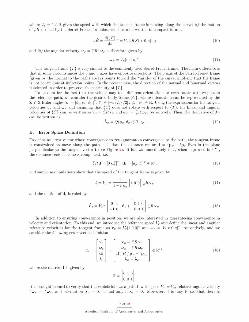
Bearing in mind that the goal of this work is to design a controller that steers the vehicle along a desiredpath, while satisfying a coordinate turn constraint, we describe in this section the transformation appliedto the vehicle dynamic model (5), which results in an error dynamic model that can be used for controlpurposes. This error dynamic model follows closely the framework defined in Reference 8. In order to definethis error space, we must first introduce two coordinate frames relating the vehicle and the desired path,Γ. These are the tangent frame {T } and the desired body frame {C}, shown in Figure 2. Both coordinateframes move along the path attached to the point on the reference path closest to the vehicle. The differencebetween the two lies in the fact that {T } is always aligned with the tangent to the path, whereas {C}provides the desired body orientation.

Figure 2. Coordinate frames: inertial {I}, body {B}, tangent {T}, and desired body frame {C}

A. The Tangent Frame {T } and Desired Body Frame {C}Let the desired path Γ be a smooth three-dimensional curve parameterized by the arc-length s. The tangentframe {T } can be defined as a coordinate frame that moves along Γ and whose orientation relative to {I} isgiven by

I

TR(s) = [t(s) n(s) b(s)] ∈ SO(3), (8)

where t(s) is the tangent, n(s) the signed normal, and b(s) the binormal to the path at the point specifiedby s. A formal definition of the tangent coordinate frame {T } and a derivation of the equations ruling itsmotion along the curve can be found in Reference 8.

According to the definition of {T }, it is straightforward to show that i) the linear velocity vT = T

IR I pT ∈

R3 takes the form

vT = VT [1 0 0]T , (9)

5 of 19


where VT = s ∈ R gives the speed with which the tangent frame is moving along the curve; ii) the motionof I

TR is ruled by the Serret-Frenet formulas, which can be written in compact form as

I

TR =

d(I

TR)

dss = VT

I

TRS([τ 0 κ]T ); (10)

and iii) the angular velocity ωT = T

IR IωT is therefore given by

ωT = VT [τ 0 κ]T . (11)

The tangent frame {T } is very similar to the commonly used Serret-Frenet frame. The main difference isthat in some circumstances the y and z axes have opposite directions. The y axis of the Serret-Frenet frame(given by the normal to the path) always points toward the “inside” of the curve, implying that the frameis not continuous at inflection points. In the present case, the direction of the normal and binormal vectorsis selected in order to preserve the continuity of {T }.

To account for the fact that the vehicle may take different orientations or even rotate with respect tothe reference path, we consider the desired body frame {C}, whose orientation can be represented by theZ-Y-X Euler angles λC = [φC θC ψC]

T, θC ∈ ]−π/2, π/2[ , φC, ψC ∈ R. Using the expressions for the tangent

velocities vT and ωT and assuming that {C} does not rotate with respect to {T }, the linear and angularvelocities of {C} can be written as vC = C

TRvT and ωC = C

TRωT , respectively. Then, the derivative of λC

can be written asλC = Q(φC, θC) C

TRωT . (12)

B. Error Space Definition

To define an error vector whose convergence to zero guarantees convergence to the path, the tangent frameis constrained to move along the path such that the distance vector d = IpB − IpT lives in the planeperpendicular to the tangent vector t (see Figure 2). It follows immediately that, when expressed in {T },the distance vector has no x-component, i.e.

T

IRd = [0 dT

t ]T , dt = [dy dz ]T ∈ R

2, (13)

and simple manipulations show that the speed of the tangent frame is given by

s = VT =1

1 − κ dy

[

1 0 0]

T

BRvB (14)

and the motion of dt is ruled by

dt = VT τ

[

0 1

−1 0

]

dt +

[

0 1 0

0 0 1

]

T

BRvB . (15)

In addition to ensuring convergence in position, we are also interested in guaranteeing convergence invelocity and orientation. To this end, we introduce the reference speed Vr and define the linear and angularreference velocities for the tangent frame as vr = Vr [1 0 0]T and ωr = Vr [τ 0 κ]T , respectively, and weconsider the following error vector definition

xe =

ve

ωe

dt

λe

=

vB − C

TRvr

ωB − C

TRωr

Π T

IR (IpB − IpT )

λB − λC

∈ R11, (16)

where the matrix Π is given by

Π =

[

0 1 0

0 0 1

]

.

It is straightforward to verify that the vehicle follows a path Γ with speed VT = Vr, relative angular velocityT ωB = T ωC, and orientation λB = λC if and only if xe = 0. Moreover, it is easy to see that there is

6 of 19


a nonlinear transformation between the original state vector xB = [vT

BωT

B

IpT

BλT

B]T ∈ R

12 and the statevector given by [xT

e s]T and that, in general, the time derivative of xe will take the form xe = fe(xe, s,u,w).However, we will see shortly that the dependence on the arc-length s can be eliminated by restricting thereferences to satisfy a trimming condition.

It is well know that a vehicle with dynamics described by (5) is said to satisfy a trimming conditionif vB = 0, ωB = 0, and u = 0 with w = 0, or equivalently, if the vehicle follows a straight line path ora z-aligned helix with constant speed and constant orientation relative to the path. Then, the referenceis guaranteed to satisfy a trimming condition if Vr = 0, κ = 0, τ = 0, T ωC = 0, λT = [0 γT ψT ]T , andψT = sign(κ)VT

√κ2 + τ2. For helices, the flight path angle is given by γT = atan(−τ/κ), whereas for

straight lines γT is a predefined constant. Under these constraints, the error dynamics can be written as

ve = f (vB, ωB, u, w) + fg (φB , θB)

ωe = n (vB, ωB, u, w)

dt = VT τ

[

0 1

−1 0

]

dt +

[

0 1 0

0 0 1

]

T

BRve

λe = Q(φB , θB)ωB − sign(κ)VT

√

κ2 + τ2 [ 0 0 1 ]T

. (17)

A simple inspection of (17) reveals that no term depends explicitly on s. Even the rotation T

BR, which

apparently depends on ψT (s) can be rewritten as T

BR = RY (θT )TRZ(ψct + ψe)RY (θB)RX(φB), where ψct

denotes the constant difference ψC − ψT . Therefore, the error state equations can be written in compactform as

xe = fe(xe,η,u), (18)

where the constant vector η = [Vr, ψr, γT , ψct, φC , θC]T completely characterizes the reference trimmingcondition.

C. The Coordinate Turn Constraint

As referred earlier in the text, it is well-known that an aircraft can describe a z-aligned helix at constantspeed and constant orientation relative to the path, while satisfying a trimming condition. In this work, weare also interested in enforcing a coordinated turn constraint.

Though in the case of small UAVs the question of ensuring the comfort of passengers is not present,implementing a coordinated turn constraint to describe a turning maneuver continues to be a relevantsolution. It brings benefits in terms of efficiency and robustness due to the rudder’s small size and does notrequire explicit dynamic inversion computations that are required to obtain, in real time, the steady statevalues for the actuators about other steady turn trimming conditions.

An aircraft is said to describe a coordinated turn maneuver if it verifies a trimming condition and theaerodynamical forces have no component along the y-axis of the body frame. Since at trimming the bodyvelocities and control input satisfy vB = 0, ωB = 0, and u = 0, we can rewrite the Newton equation givenin (4) as

S(ωB)mvB = faero(vB,ωB,u,w) + fg(φB, θB).

Then, the coordinated turn condition is verified if the aircraft’s orientation is such that [0 1 0]faero = 0 andconsequently the y-components of the gravitational and centripetal forces coincide, that is,

[0 1 0]S(ωB)mvB = [0 1 0]fg(φB , θB). (19)

Assuming that the trimming condition is specified by the linear speed Vr, curvature κ, torsion τ , roll angle φC ,pitch angle θC , and yaw angle relative to the path ψct, then the body velocities can be written as vB = C

TRvr

and ωB = C

TRωr, where vr = Vr[1 0 0]T , ωr = Vr[τ 0 κ]T , and C

TR = RX(φC)TRY (θC)TRZ(ψct)

TRY (γT ).Therefore (19) takes the form

eT

2C

TRS(ωr)vr = eT

2RX(φC)TRY (θC)T ge3

⇔eT

2RX(φC)TRY (θC)T (RZ(ψct)TV 2

r κe2 − ge3) = 0(20)

where e2 = [0 1 0]T and e3 = [0 0 1]T .

7 of 19


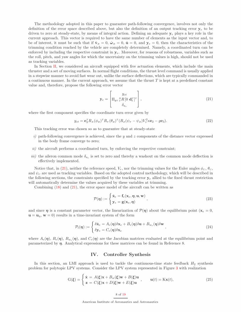
The methodology adopted in this paper to guarantee path-following convergence, involves not only thedefinition of the error space described above, but also the definition of an output tracking error ye to bedriven to zero at steady-state, by means of integral action. Defining an adequate ye plays a key role in thecurrent approach. This vector is required to have the same number of elements as the input vector and, tobe of interest, it must be such that if vB = 0, ωB = 0, u = 0, and ye = 0, then the characteristics of thetrimming condition reached by the vehicle are completely determined. Namely, a coordinated turn can beenforced by including the respective constraint in ye. Moreover, for reasons of robustness, variables such asthe roll, pitch, and yaw angles for which the uncertainty on the trimming values is high, should not be usedas tracking variables.

In Section II, we considered an aircraft equipped with five actuation elements, which include the mainthruster and a set of moving surfaces. In normal flight conditions, the thrust level command is usually appliedin a stepwise manner to avoid fast wear out, unlike the surface deflections, which are typically commanded ina continuous manner. In the current approach, we assume that the thrust T is kept at a predefined constantvalue and, therefore, propose the following error vector

ye =

yct

ΠyzB

TR [0 dT

t ]T

δac

, (21)

where the first component specifies the coordinate turn error given by

yct = eT

2RX(φB)TRY (θB)T (RZ(ψT − ψB)V 2Tκe2 − ge3). (22)

This tracking error was chosen so as to guarantee that at steady-state

i) path-following convergence is achieved, since the y and z components of the distance vector expressedin the body frame converge to zero;

ii) the aircraft performs a coordinated turn, by enforcing the respective constraint;

iii) the aileron common mode δacis set to zero and thereby a washout on the common mode deflection is

effectively implemented.

Notice that, in (21), neither the reference speed, Vr , nor the trimming values for the Euler angles φC , θC,and ψC are used as tracking variables. Based on the adopted control methodology, which will be described inthe following sections, the constraints specified by the tracking error ye allied to the fixed thrust restrictionwill automatically determine the values acquired by these variables at trimming.

Combining (18) and (21), the error space model of the aircraft can be written as

P(η) :=

{

xe = fe(xe,η,u,w)

ye = g(xe,η), (23)

and since η is a constant parameter vector, the linearization of P(η) about the equilibrium point (xe = 0,u = uη, w = 0) results in a time-invariant system of the form

Pl(η) :=

{

δxe = Ae(η)δxe +Be(η)δu +Bwe(η)δw

δye = Ce(η)δxe

, (24)

where Ae(η), Be(η), Bwe(η), and Ce(η) are the Jacobian matrices evaluated at the equilibrium point and

parameterized by η. Analytical expressions for these matrices can be found in Reference 8.

IV. Controller Synthesis

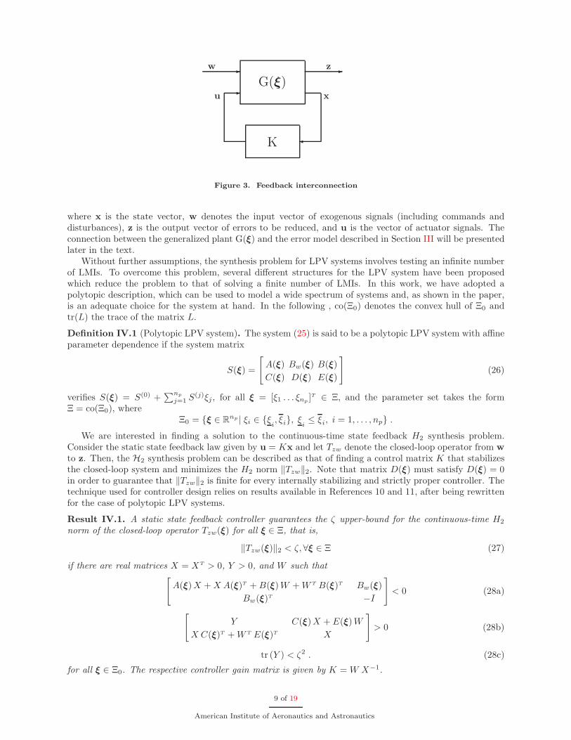
In this section, an LMI approach is used to tackle the continuous-time state feedback H2 synthesisproblem for polytopic LPV systems. Consider the LPV system represented in Figure 3 with realization

G(ξ) =

{

x = A(ξ)x +Bw(ξ)w +B(ξ)u

z = C(ξ)x +D(ξ)w + E(ξ)u, u(t) = Kx(t), (25)

8 of 19


K

-

G(ξ)

�

--w z

xu

Figure 3. Feedback interconnection

where x is the state vector, w denotes the input vector of exogenous signals (including commands anddisturbances), z is the output vector of errors to be reduced, and u is the vector of actuator signals. Theconnection between the generalized plant G(ξ) and the error model described in Section III will be presentedlater in the text.

Without further assumptions, the synthesis problem for LPV systems involves testing an infinite numberof LMIs. To overcome this problem, several different structures for the LPV system have been proposedwhich reduce the problem to that of solving a finite number of LMIs. In this work, we have adopted apolytopic description, which can be used to model a wide spectrum of systems and, as shown in the paper,is an adequate choice for the system at hand. In the following , co(Ξ0) denotes the convex hull of Ξ0 andtr(L) the trace of the matrix L.

Definition IV.1 (Polytopic LPV system). The system (25) is said to be a polytopic LPV system with affineparameter dependence if the system matrix

S(ξ) =

[

A(ξ) Bw(ξ) B(ξ)

C(ξ) D(ξ) E(ξ)

]

(26)

verifies S(ξ) = S(0) +∑np

j=1 S(j)ξj , for all ξ = [ξ1 . . . ξnp

]T ∈ Ξ, and the parameter set takes the formΞ = co(Ξ0), where

Ξ0 = {ξ ∈ Rnp | ξi ∈ {ξ

i, ξi}, ξi

≤ ξi, i = 1, . . . , np} .We are interested in finding a solution to the continuous-time state feedback H2 synthesis problem.

Consider the static state feedback law given by u = Kx and let Tzw denote the closed-loop operator from w

to z. Then, the H2 synthesis problem can be described as that of finding a control matrix K that stabilizesthe closed-loop system and minimizes the H2 norm ‖Tzw‖2. Note that matrix D(ξ) must satisfy D(ξ) = 0in order to guarantee that ‖Tzw‖2 is finite for every internally stabilizing and strictly proper controller. Thetechnique used for controller design relies on results available in References 10 and 11, after being rewrittenfor the case of polytopic LPV systems.

Result IV.1. A static state feedback controller guarantees the ζ upper-bound for the continuous-time H2

norm of the closed-loop operator Tzw(ξ) for all ξ ∈ Ξ, that is,

‖Tzw(ξ)‖2 < ζ, ∀ξ ∈ Ξ (27)

if there are real matrices X = XT > 0, Y > 0, and W such that[

A(ξ)X +X A(ξ)T +B(ξ)W +W T B(ξ)T Bw(ξ)

Bw(ξ)T −I

]

< 0 (28a)

[

Y C(ξ)X + E(ξ)W

X C(ξ)T +W T E(ξ)T X

]

> 0 (28b)

tr (Y ) < ζ2 . (28c)

for all ξ ∈ Ξ0. The respective controller gain matrix is given by K = W X−1.

9 of 19


Additional closed-loop regional eigenvalues placement specifications for each plant G(ξ) in the polytopicregion identified with the parameter set Ξ can also be converted into design constraints resorting to theconcept of LMI regions in the complex plane introduced in Reference 18. These constitute a generalizationof the well known α stability region presented next.

Result IV.2. The closed-loop system with realization (25) has all the eigenvalues in the semi-plane λ ∈ C :Re(λ) < −α for all ξ ∈ Ξ if matrices X = XT > 0 and W exist such that the closed-loop Lyapunov inequality

A(ξ)X +X A(ξ)T +B(ξ)W +W T B(ξ)T + 2αI < 0 (29)

is satisfied for all ξ ∈ Ξ0.

This well known result can be generalized as follows. Let L = [lij ] and M = [mij ] be real symmetricmatrices. An LMI region Rlmi is defined as an open domain in the complex plane that satisfies

Rlmi = {z ∈ C : lij +mijz +mjiz < 0; i, j = 1, ..., n} . (30)

This description can represent a large number of regions which are symmetric with respect to the real axis,such as conic sectors, half-planes, etc. Using the concept of LMI regions, Result IV.2 admits the followinggeneralization, see Reference 18 for further details:

Result IV.3. The closed-loop system with realization (25) has all the eigenvalues in the region Rcl definedby (30) for all ξ ∈ Ξ if a real symmetric matrix X > 0 exists such that the closed-loop generalized Lyapunovinequality

lijX +mij(A(ξ)X +B(ξ)W ) +mji(X A(ξ)T +W T B(ξ)T ) < 0; i, j = 1, ..., n. (31)

is satisfied.

θreg

Im(s)

Re(s)−αreg

Figure 4. A typical closed-loop generalized stability region

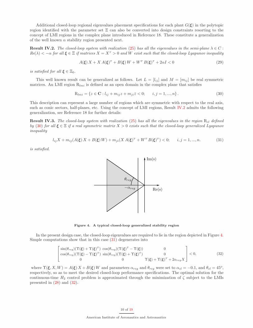
In the present design case, the closed-loop eigenvalues are required to lie in the region depicted in Figure 4.Simple computations show that in this case (31) degenerates into

sin(θreg)(Υ(ξ) + Υ(ξ)T ) cos(θreg)(Υ(ξ)T− Υ(ξ)) 0

cos(θreg)(Υ(ξ) − Υ(ξ)T ) sin(θreg)(Υ(ξ) + Υ(ξ)T ) 0

0 0 Υ(ξ) + Υ(ξ)T + 2αregX

< 0, (32)

where Υ(ξ, X,W ) = A(ξ)X +B(ξ)W and parameters αreg and θreg were set to αcl = −0.1, and θcl = 45o,respectively, so as to meet the desired closed-loop performance specifications. The optimal solution for thecontinuous-time H2 control problem is approximated through the minimization of ζ subject to the LMIspresented in (28) and (32).

10 of 19


A. Affine Parameter Dependent Approximation of the Error Dynamics

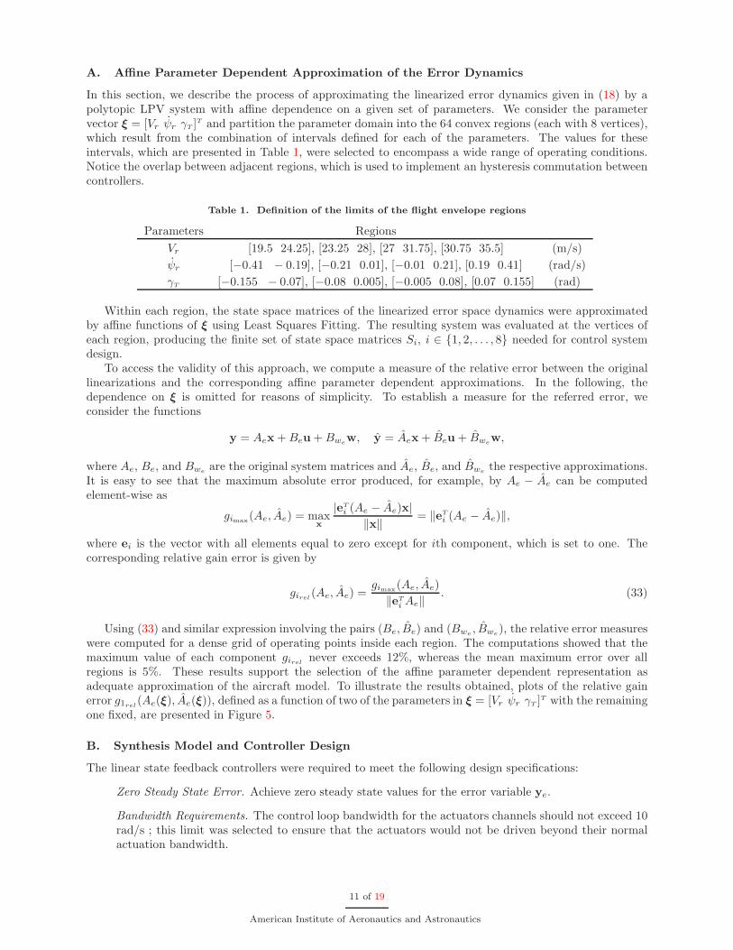
In this section, we describe the process of approximating the linearized error dynamics given in (18) by apolytopic LPV system with affine dependence on a given set of parameters. We consider the parametervector ξ = [Vr ψr γT ]T and partition the parameter domain into the 64 convex regions (each with 8 vertices),which result from the combination of intervals defined for each of the parameters. The values for theseintervals, which are presented in Table 1, were selected to encompass a wide range of operating conditions.Notice the overlap between adjacent regions, which is used to implement an hysteresis commutation betweencontrollers.

Table 1. Definition of the limits of the flight envelope regions

Parameters Regions

Vr [19.5 24.25], [23.25 28], [27 31.75], [30.75 35.5] (m/s)

ψr [−0.41 − 0.19], [−0.21 0.01], [−0.01 0.21], [0.19 0.41] (rad/s)

γT [−0.155 − 0.07], [−0.08 0.005], [−0.005 0.08], [0.07 0.155] (rad)

Within each region, the state space matrices of the linearized error space dynamics were approximatedby affine functions of ξ using Least Squares Fitting. The resulting system was evaluated at the vertices ofeach region, producing the finite set of state space matrices Si, i ∈ {1, 2, . . . , 8} needed for control systemdesign.

To access the validity of this approach, we compute a measure of the relative error between the originallinearizations and the corresponding affine parameter dependent approximations. In the following, thedependence on ξ is omitted for reasons of simplicity. To establish a measure for the referred error, weconsider the functions

y = Aex +Beu +Bwew, y = Aex + Beu + Bwe

w,

where Ae, Be, and Bweare the original system matrices and Ae, Be, and Bwe

the respective approximations.It is easy to see that the maximum absolute error produced, for example, by Ae − Ae can be computedelement-wise as

gimax(Ae, Ae) = max

x

|eT

i (Ae − Ae)x|‖x‖ = ‖eT

i (Ae − Ae)‖,

where ei is the vector with all elements equal to zero except for ith component, which is set to one. Thecorresponding relative gain error is given by

girel(Ae, Ae) =

gimax(Ae, Ae)

‖eT

i Ae‖. (33)

Using (33) and similar expression involving the pairs (Be, Be) and (Bwe, Bwe

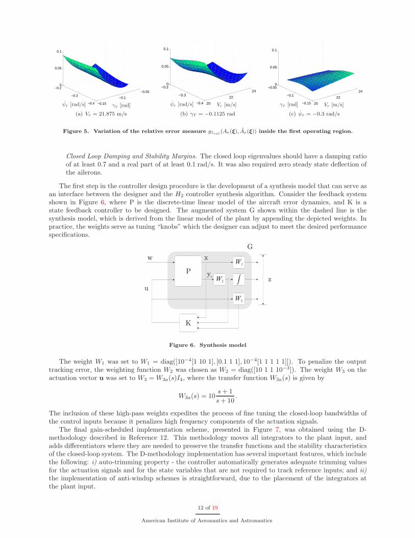
), the relative error measureswere computed for a dense grid of operating points inside each region. The computations showed that themaximum value of each component girel

never exceeds 12%, whereas the mean maximum error over allregions is 5%. These results support the selection of the affine parameter dependent representation asadequate approximation of the aircraft model. To illustrate the results obtained, plots of the relative gainerror g1rel

(Ae(ξ), Ae(ξ)), defined as a function of two of the parameters in ξ = [Vr ψr γT ]T with the remainingone fixed, are presented in Figure 5.

B. Synthesis Model and Controller Design

The linear state feedback controllers were required to meet the following design specifications:

Zero Steady State Error. Achieve zero steady state values for the error variable ye.

Bandwidth Requirements. The control loop bandwidth for the actuators channels should not exceed 10rad/s ; this limit was selected to ensure that the actuators would not be driven beyond their normalactuation bandwidth.

11 of 19


−0.15

−0.1

−0.05

−0.4

−0.3

−0.20

0.05

0.1

ψr [rad/s] γT [rad]

(a) Vr = 21.875 m/s

20

22

24

−0.4

−0.3

−0.20

0.05

0.1

ψr [rad/s] Vr [m/s]

(b) γT = −0.1125 rad

20

22

24

−0.15

−0.1

−0.050

0.05

0.1

γT [rad] Vr [m/s]

(c) ψr = −0.3 rad/s

Figure 5. Variation of the relative error measure g1rel(Ae(ξ), Ae(ξ)) inside the first operating region.

Closed Loop Damping and Stability Margins. The closed loop eigenvalues should have a damping ratioof at least 0.7 and a real part of at least 0.1 rad/s. It was also required zero steady state deflection ofthe ailerons.

The first step in the controller design procedure is the development of a synthesis model that can serve asan interface between the designer and the H2 controller synthesis algorithm. Consider the feedback systemshown in Figure 6, where P is the discrete-time linear model of the aircraft error dynamics, and K is astate feedback controller to be designed. The augmented system G shown within the dashed line is thesynthesis model, which is derived from the linear model of the plant by appending the depicted weights. Inpractice, the weights serve as tuning “knobs” which the designer can adjust to meet the desired performancespecifications.

P

W3

K

ye

u

w

G

W2

xW

1

zZZ

Figure 6. Synthesis model

The weight W1 was set to W1 = diag([10−4[1 10 1], [0.1 1 1], 10−4[1 1 1 1 1]]). To penalize the outputtracking error, the weighting function W2 was chosen as W2 = diag([10 1 1 10−3]). The weight W3 on theactuation vector u was set to W3 = W3a(s)I4, where the transfer function W3a(s) is given by

W3a(s) = 10s+ 1

s+ 10.

The inclusion of these high-pass weights expedites the process of fine tuning the closed-loop bandwidths ofthe control inputs because it penalizes high frequency components of the actuation signals.

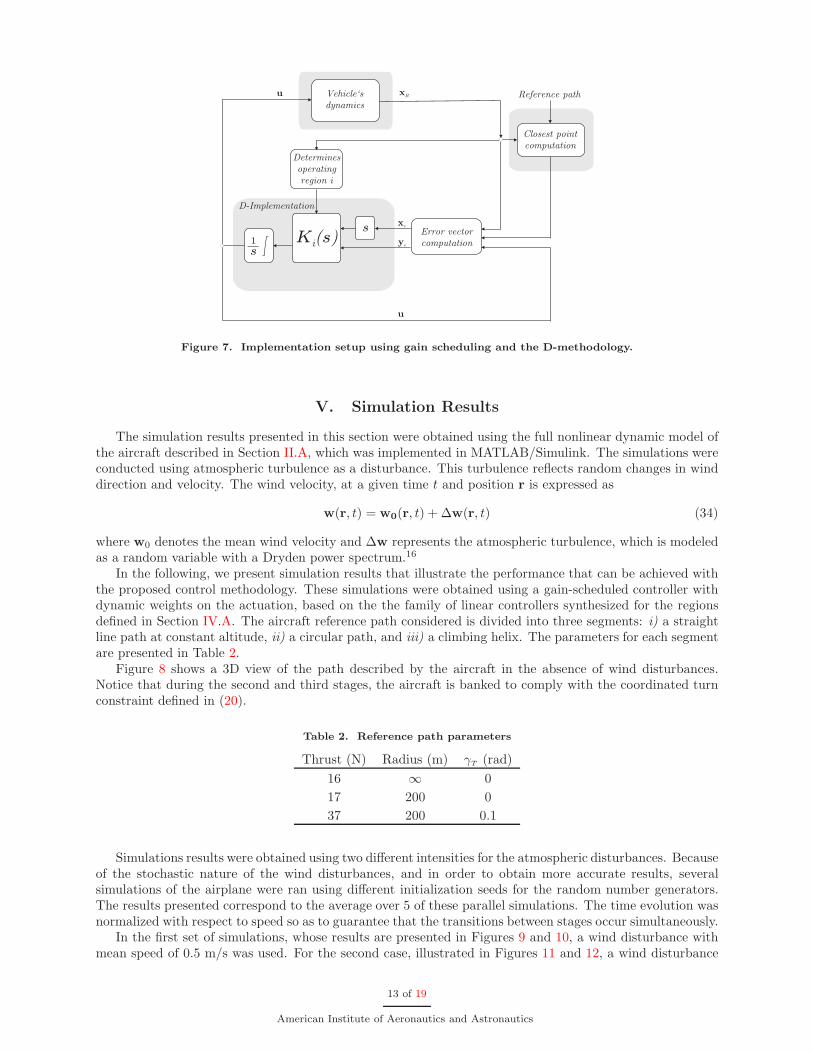
The final gain-scheduled implementation scheme, presented in Figure 7, was obtained using the D-methodology described in Reference 12. This methodology moves all integrators to the plant input, andadds differentiators where they are needed to preserve the transfer functions and the stability characteristicsof the closed-loop system. The D-methodology implementation has several important features, which includethe following: i) auto-trimming property - the controller automatically generates adequate trimming valuesfor the actuation signals and for the state variables that are not required to track reference inputs; and ii)the implementation of anti-windup schemes is straightforward, due to the placement of the integrators atthe plant input.

12 of 19


Vehicle`sdynamics

u xB

Error vectorcomputation

Determinesoperatingregion i

xe

D-Implementation

Reference path

Closest pointcomputation

ye

u

s

1

s

K si( )

Figure 7. Implementation setup using gain scheduling and the D-methodology.

V. Simulation Results

The simulation results presented in this section were obtained using the full nonlinear dynamic model ofthe aircraft described in Section II.A, which was implemented in MATLAB/Simulink. The simulations wereconducted using atmospheric turbulence as a disturbance. This turbulence reflects random changes in winddirection and velocity. The wind velocity, at a given time t and position r is expressed as

w(r, t) = w0(r, t) + ∆w(r, t) (34)

where w0 denotes the mean wind velocity and ∆w represents the atmospheric turbulence, which is modeledas a random variable with a Dryden power spectrum.16

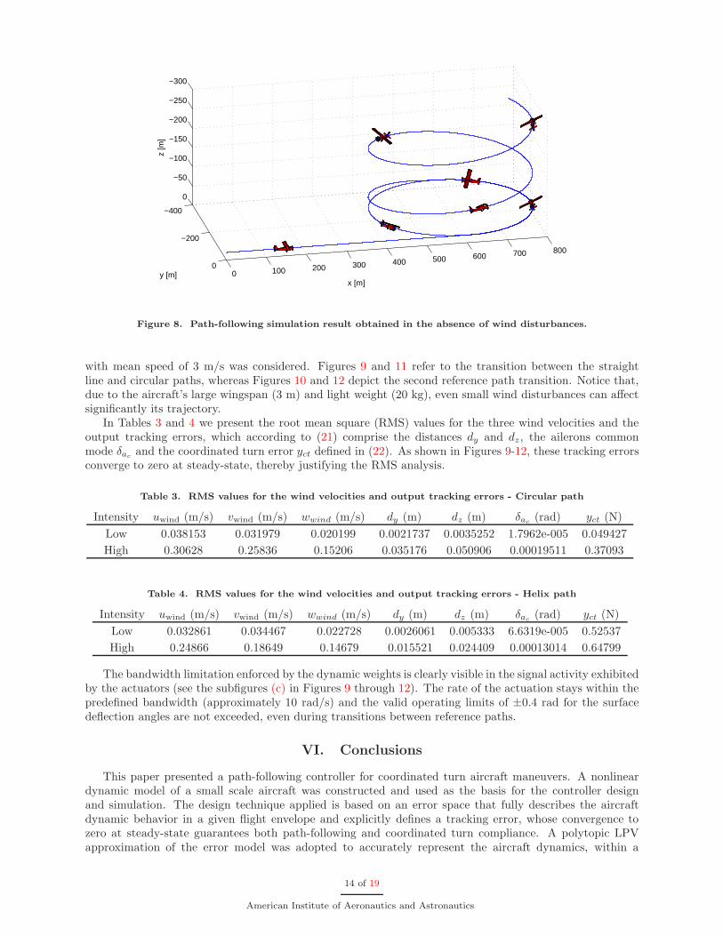
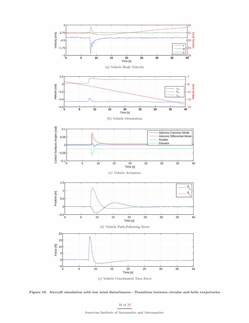
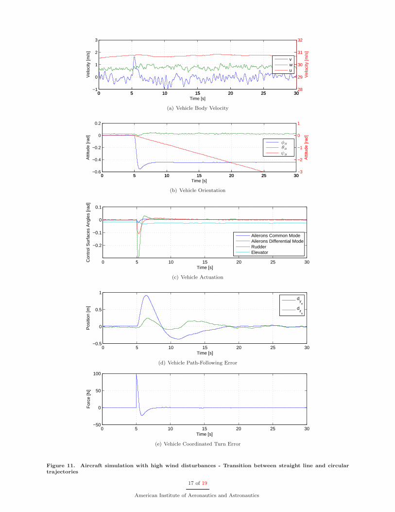
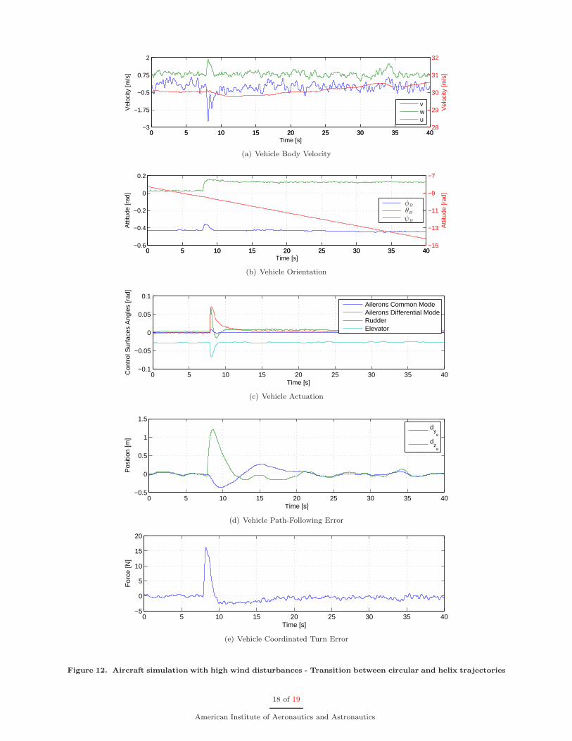
In the following, we present simulation results that illustrate the performance that can be achieved withthe proposed control methodology. These simulations were obtained using a gain-scheduled controller withdynamic weights on the actuation, based on the the family of linear controllers synthesized for the regionsdefined in Section IV.A. The aircraft reference path considered is divided into three segments: i) a straightline path at constant altitude, ii) a circular path, and iii) a climbing helix. The parameters for each segmentare presented in Table 2.

Figure 8 shows a 3D view of the path described by the aircraft in the absence of wind disturbances.Notice that during the second and third stages, the aircraft is banked to comply with the coordinated turnconstraint defined in (20).

Table 2. Reference path parameters

Thrust (N) Radius (m) γT (rad)

16 ∞ 0

17 200 0

37 200 0.1

Simulations results were obtained using two different intensities for the atmospheric disturbances. Becauseof the stochastic nature of the wind disturbances, and in order to obtain more accurate results, severalsimulations of the airplane were ran using different initialization seeds for the random number generators.The results presented correspond to the average over 5 of these parallel simulations. The time evolution wasnormalized with respect to speed so as to guarantee that the transitions between stages occur simultaneously.

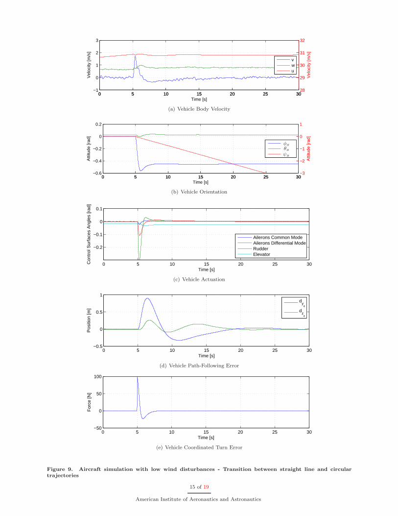
In the first set of simulations, whose results are presented in Figures 9 and 10, a wind disturbance withmean speed of 0.5 m/s was used. For the second case, illustrated in Figures 11 and 12, a wind disturbance

13 of 19


0 100 200 300 400 500 600 700 800

−400

−200

0

−300

−250

−200

−150

−100

−50

0

x [m]y [m]

z [m

]

Figure 8. Path-following simulation result obtained in the absence of wind disturbances.

with mean speed of 3 m/s was considered. Figures 9 and 11 refer to the transition between the straightline and circular paths, whereas Figures 10 and 12 depict the second reference path transition. Notice that,due to the aircraft’s large wingspan (3 m) and light weight (20 kg), even small wind disturbances can affectsignificantly its trajectory.

In Tables 3 and 4 we present the root mean square (RMS) values for the three wind velocities and theoutput tracking errors, which according to (21) comprise the distances dy and dz, the ailerons commonmode δac

and the coordinated turn error yct defined in (22). As shown in Figures 9-12, these tracking errorsconverge to zero at steady-state, thereby justifying the RMS analysis.

Table 3. RMS values for the wind velocities and output tracking errors - Circular path

Intensity uwind (m/s) vwind (m/s) wwind (m/s) dy (m) dz (m) δac(rad) yct (N)

Low 0.038153 0.031979 0.020199 0.0021737 0.0035252 1.7962e-005 0.049427

High 0.30628 0.25836 0.15206 0.035176 0.050906 0.00019511 0.37093

Table 4. RMS values for the wind velocities and output tracking errors - Helix path

Intensity uwind (m/s) vwind (m/s) wwind (m/s) dy (m) dz (m) δac(rad) yct (N)

Low 0.032861 0.034467 0.022728 0.0026061 0.005333 6.6319e-005 0.52537

High 0.24866 0.18649 0.14679 0.015521 0.024409 0.00013014 0.64799

The bandwidth limitation enforced by the dynamic weights is clearly visible in the signal activity exhibitedby the actuators (see the subfigures (c) in Figures 9 through 12). The rate of the actuation stays within thepredefined bandwidth (approximately 10 rad/s) and the valid operating limits of ±0.4 rad for the surfacedeflection angles are not exceeded, even during transitions between reference paths.

VI. Conclusions

This paper presented a path-following controller for coordinated turn aircraft maneuvers. A nonlineardynamic model of a small scale aircraft was constructed and used as the basis for the controller designand simulation. The design technique applied is based on an error space that fully describes the aircraftdynamic behavior in a given flight envelope and explicitly defines a tracking error, whose convergence tozero at steady-state guarantees both path-following and coordinated turn compliance. A polytopic LPVapproximation of the error model was adopted to accurately represent the aircraft dynamics, within a

14 of 19


0 5 10 15 20 25 30−1

0

1

2

3

Vel

ocity

[m/s

]

Time [s]

0 5 10 15 20 25 3028

29

30

31

32

Vel

ocity

[m/s

]

vwu

(a) Vehicle Body Velocity

0 5 10 15 20 25 30−0.6

−0.4

−0.2

0

0.2

Atti

tude

[rad

]

Time [s]

0 5 10 15 20 25 30−3

−2

−1

0

1

Atti

tude

[rad

]

φB

θB

ψB

(b) Vehicle Orientation

0 5 10 15 20 25 30

−0.2

−0.1

0

0.1

Time [s]

Con

trol

Sur

face

s A

ngle

s [r

ad]

Ailerons Common ModeAilerons Differential ModeRudderElevator

(c) Vehicle Actuation

0 5 10 15 20 25 30−0.5

0

0.5

1

Time [s]

Pos

ition

[m]

d

ye

dz

e

(d) Vehicle Path-Following Error

0 5 10 15 20 25 30−50

0

50

100

Time [s]

For

ce [N

]

(e) Vehicle Coordinated Turn Error

Figure 9. Aircraft simulation with low wind disturbances - Transition between straight line and circular

trajectories

15 of 19


0 5 10 15 20 25 30 35 40−3

−1.75

−0.5

0.75

2

Vel

ocity

[m/s

]

Time [s]

0 5 10 15 20 25 30 35 4028

29

30

31

32

Vel

ocity

[m/s

]

vwu


0 5 10 15 20 25 30 35 40−0.6

−0.4

−0.2

0

0.2

Atti

tude

[rad

]

Time [s]

0 5 10 15 20 25 30 35 40−15

−13

−11

−9

−7

Atti

tude

[rad

]

φB

θB

ψB


0 5 10 15 20 25 30 35 40−0.1

−0.05

0

0.05

0.1

Time [s]

Con

trol

Sur

face

s A

ngle

s [r

ad]



0 5 10 15 20 25 30 35 40−0.5

0

0.5

1

1.5

Time [s]

Pos

ition

[m]

d

ye

dz

e


0 5 10 15 20 25 30 35 40−5

0

5

10

15

20

Time [s]

For

ce [N

]


Figure 10. Aircraft simulation with low wind disturbances - Transition between circular and helix trajectories

16 of 19


0 5 10 15 20 25 30−1

0

1

2

3

Vel

ocity

[m/s

]

Time [s]

0 5 10 15 20 25 3028

29

30

31

32

Vel

ocity

[m/s

]

vwu


0 5 10 15 20 25 30−0.6

−0.4

−0.2

0

0.2

Atti

tude

[rad

]

Time [s]

0 5 10 15 20 25 30−3

−2

−1

0

1

Atti

tude

[rad

]

φB

θB

ψB


0 5 10 15 20 25 30

−0.2

−0.1

0

0.1

Time [s]

Con

trol

Sur

face

s A

ngle

s [r

ad]



0 5 10 15 20 25 30−0.5

0

0.5

1

Time [s]

Pos

ition

[m]

d

ye

dz

e


0 5 10 15 20 25 30−50

0

50

100

Time [s]

For

ce [N

]


Figure 11. Aircraft simulation with high wind disturbances - Transition between straight line and circular

trajectories

17 of 19


0 5 10 15 20 25 30 35 40−3

−1.75

−0.5

0.75

2

Vel

ocity

[m/s

]

Time [s]

0 5 10 15 20 25 30 35 4028

29

30

31

32

Vel

ocity

[m/s

]

vwu


0 5 10 15 20 25 30 35 40−0.6

−0.4

−0.2

0

0.2

Atti

tude

[rad

]

Time [s]

0 5 10 15 20 25 30 35 40−15

−13

−11

−9

−7

Atti

tude

[rad

]

φB

θB

ψB


0 5 10 15 20 25 30 35 40−0.1

−0.05

0

0.05

0.1

Time [s]

Con

trol

Sur

face

s A

ngle

s [r

ad]



0 5 10 15 20 25 30 35 40−0.5

0

0.5

1

1.5

Time [s]

Pos

ition

[m]

d

ye

dz

e


0 5 10 15 20 25 30 35 40−5

0

5

10

15

20

Time [s]

For

ce [N

]


Figure 12. Aircraft simulation with high wind disturbances - Transition between circular and helix trajectories

18 of 19


predefined set of operating regions. An LMI-based H2 controller design methodology for polytopic LPVsystems was applied, which includes pole placement constraints and exploits dynamic weights to limit theactuation bandwidth. The full nonlinear controller was implemented using gain-scheduling control theoryand tested in simulation with the nonlinear model of a small scale airplane. The simulation results obtainedattest to the adequacy of the proposed path-following control methodology.

Acknowledgments

This work was partially supported by Fundacao para a Ciencia e a Tecnologia (ISR/IST pluriannualfunding) through the POS Conhecimento Program that includes FEDER funds.

References

1Azam, S. N. and Singh, M., “Invertibility and Trajectory Control for Nonlinear Maneuvers of Aircraft,” AIAA Journalof Guidance, Control, and Dynamics, Vol. 17, No. 1, 1994, pp. 192–200.

2Al-Hiddabi, N. H. and McClamrooh, S. A., “Trajectory tracking control and maneuver regulation control for the CTOLaircraft model,” Decision and Control, 1999. Proceedings of the 38th IEEE Conference on, Vol. 2, 1999, pp. 1958–1963.

3Shue, S.-P., Sawan, M. E., and Rokhsaz, K., “Mixed H2/H∞ Method Suitable for Gain Scheduled Aircraft Control,”Journal of Guidance, Control, and Dynamics 1997 , Vol. 20, No. 4, 1999, pp. 699–706.

4Thompson, P. and Chiang, R., “H∞ robust control synthesis for a fighter performing a coordinated bank turn,” Decisionand Control, 1990., Proceedings of the 29th IEEE Conference on, Praha, Czech Republic, 1990.

5Stevens, B. L. and Lewis, F. L., Aircraft Control and Simulation, 2nd Edition, Wiley-Interscience, 2003.6Kaminer, I., Pascoal, A., Hallberg, E., and Silvestre, C., “Trajectory Tracking for Autonomous Vehicles: An Integrated

Approach to Guidance and Control,” AIAA Journal of Guidance, Control, and Dynamics, Vol. 21, No. 1, 1998, pp. 29–38.7Silvestre, C., Pascoal, A., and Kaminer, I., “On the Design of Gain-Scheduled Trajectory Tracking Controllers,” Inter-

national Journal of Robust and Nonlinear Control , Vol. 12, 2002, pp. 797–839.8Cunha, R., Antunes, D., Gomes, P., and Silvestre, C., “A Path-Following Preview Controller for Autonomous Air

Vehicles,” AIAA Guidance Navigation and Control Conference, Keystone, CO, USA, 2006.9Boyd, S., Ghaoui, L. E., Feron, E., and Balakrishnan, V., Linear Matrix Inequalities in Systems and Control Theory ,

Society for Industrial and Applied Mathematics, SIAM, Philadelphia, PA, 1994.10Ghaoui, L. E. and Niculescu, S. I., editors, Advances in Linear Matrix Inequality Methods in Control , Society for

Industrial and Applied Mathematics, SIAM, Philadelphia, PA, 1999.11Scherer, C. and Weiland, S., Lecture Notes on Linear Matrix Inequalities in Control , Dutch Institute of Systems and

Control, 2000.12Kaminer, I., Pascoal, A., Khargonekar, P., and Coleman, E., “A Velocity Algorithm for the Implementation of Gain-

Scheduled Controllers,” Automatica, Vol. 31, No. 8, 1995, pp. 1185–1191.13Craig, J. J., Introduction to Robotics and Control: Mechanics and Control, 2nd ed., Addison-Wesley Publishing Company,

Massachusetts, 1989.14Brederode, V., Fundamentos de Aerodinmica Incompressvel , Author’s publication, 1997.15Schmidt, L. V., Introduction to Aircraft Flight Dynamics, AIAA Education Series, 1998.16Stengel, R. F., Flight Dynamics, Princeton University Press, Flight Dynamics.17Rosa, P., Silvestre, C., Cabecinhas, D., and Cunha, R., “Autolanding Controller for a Fixed Wing Unmanned Air Vehicle,”

AIAA Guidance and Control Conference (Submitted), 2007.18Chilali, M. and Gahinet, P., “H∞ design with pole placement constraints: an LMI approach,” IEEE Transactions on

Automatic Control , Vol. 41, No. 3, March 1996, pp. 358–367.

19 of 19


Path-Following Control for Coordinated Turn Aircraft...

Documents

Transcript of Path-Following Control for Coordinated Turn Aircraft...