Path dependence and the validation of agent-based spatial ... · 2. An agent-based model of land...

Path dependence and the validation of agent-based spatial models ofland use

DANIEL G. BROWN*{{, SCOTT PAGE{§, RICK RIOLO{,

MOIRA ZELLNER{" and WILLIAM RAND{

{Center for the Study of Complex Systems, University of Michigan, USA

{School of Natural Resources and Environment, University of Michigan, USA

§Departments of Political Science and Economics, University of Michigan, USA

"Taubmann College of Architecture and Urban Planning, University of Michigan, USA

"Department of Electrical Engineering and Computer Science, University of Michigan,

USA

In this paper, we identify two distinct notions of accuracy of land-use models and

highlight a tension between them. A model can have predictive accuracy: its

predicted land-use pattern can be highly correlated with the actual land-use

pattern. A model can also have process accuracy: the process by which locations

or land-use patterns are determined can be consistent with real world processes.

To balance these two potentially conflicting motivations, we introduce the

concept of the invariant region, i.e., the area where land-use type is almost certain,

and thus path independent; and the variant region, i.e., the area where land use

depends on a particular series of events, and is thus path dependent. We

demonstrate our methods using an agent-based land-use model and using multi-

temporal land-use data collected for Washtenaw County, Michigan, USA. The

results indicate that, using the methods we describe, researchers can improve

their ability to communicate how well their model performs, the situations or

instances in which it does not perform well, and the cases in which it is relatively

unlikely to predict well because of either path dependence or stochastic

uncertainty.

Keywords: Agent-based modeling; Land-use change; Urban sprawl; Model

validation; Complex systems

1. Introduction

The rise of models that represent the functioning of complex adaptive systems has

led to an increased awareness of the possibility for path dependency and multiple

equilibria in economic and ecological systems in general (Pahl-Wostl 1995) and

spatial land-use systems in particular (Atkinson and Oelson 1996, Wilson 2000,

Balmann 2001). Path dependence arises from negative and positive feedbacks.

Negative feedbacks in the form of spatial dis-amenities rule out some patterns of

development and positive feedbacks from roads and other infrastructure and from

*Corresponding author. , 430 E. University Ave., Ann Arbor, MI 48109-1115, USA.Email: [email protected]

International Journal of Geographical Information Science

Vol. 19, No. 2, February 2005, 153–174

International Journal of Geographical Information ScienceISSN 1365-8816 print/ISSN 1362-3087 online # 2005 Taylor & Francis Ltd

http://www.tandf.co.uk/journalsDOI: 10.1080/13658810410001713399

service centers reinforce existing paths (Arthur 1988, Arthur 1989). Thus, a small

random component in location decisions can lead to large deviations in settlement

patterns which could not result were those feedbacks not present (Atkinson and

Oleson 1996). Concurrent with this awareness of the unpredictability of settlement

patterns has been an increased availability of spatial data within geographic

information systems (GIS). This has led to greater emphasis on the validation of

spatial land-use models (Costanza 1989, Pontius 2000, 2002, Kok et al. 2001). These

two scientific advances, one theoretical and one empirical, have lead to two

contradictory impulses in land-use modeling: the desire for increased accuracy of

prediction and the recognition of unpredictability in the process. This paper addresses

the balance between these two impulses: the desire for accuracy of prediction and

accuracy of process.

Accuracy of prediction refers to the resemblance of model output to data about

the environments and regions they are meant to describe, usually measured as either

aggregate similarity and spatial similarity. Aggregate similarity refers to similarities

in statistics that describe the mapped pattern of land use such as the distributions of

sizes of developed clusters, the functional relationship between distance to city

center and density (Batty and Longley 1994, Makse et al. 1998; Andersson et al.

2002, Rand et al. 2003), or landscape pattern metrics developed within the landscape

ecology literature (e.g., McGarigal and Marks 1995) to measure the degree of

fragmentation in the landscape (Parker and Meretsky 2004).

Spatial similarity refers to the degree of match between land-use maps and a single

run or summary of multiple runs of a land-use model. The most common

approaches build on the basic error matrix approach (Congalton 1991), by which

agreement can be summarized using the kappa statistic (Cohen 1960). Pontius

(2000) has developed map comparison methods for model validation that partitions

total errors into those due to the amounts of each land-use type and those due to

their locations. Because models rely on generalizations of reality, spatial similarity

measures must be considered in light of their scale; the coarser the partition, the

easier the matching task becomes (Constanza 1989, Kok et al. 2001, Pontius 2002

and Hagen 2003).

Because spatial patterns contain more information than can be captured by

a handful of aggregate statistics, validation using spatial similarity raises the

empirical bar over aggregate similarity. However, as we shall demonstrate in this

paper, demanding that modelers get the locations right may be asking too

much.

Human decision-making is rarely deterministic, and land-use models commonly

include stochastic processes as a result (e.g., in the use of random utility theory;

Irwin and Geoghegan 2001). Many models, therefore, produce varying results

because of stochastic uncertainty in their processes. Further, to represent the

feedback processes, land-use modelers are making increasing use of cellular

automata (Batty and Xie 1994, Clarke et al. 1996, White and Engelen 1997) and

agent-based simulation (Balmann 2001, Rand et al. 2002, Parker and Meretsky

2004). These and other modeling approaches that can represent feedbacks can

exhibit spatial path dependence, i.e., the spatial patterns that result can be very

sensitive to slight differences in processes or initial conditions. How sensitive

depends upon specific attributes of the model. Given the presence of path

dependence and the effect it can have on magnifying uncertainties in land-use

models, any model that consistently returns spatial patterns in which the locations

154 D. G. Brown et al.

of land uses are similar to the real world could be overfit, i.e., it may represent the

outcomes of a particular case well but the description of the process may not be

generalizable.

We believe that the situation creates an imposing challenge: to make accurate

predictions, but to admit the inability to be completely accurate owing to path

dependence and stochastic uncertainty. If we pursue only the first part of the dictum

at the expense of the second part, we encourage a tendency towards overfitting, in

which the model is constrained by more and more information such that its ability

to run in the absence of data (e.g., in the future) or to predict surprising results is

reduced. If we emphasize the latter, then we abandon hope of predicting those

spatial properties that are path or state invariant. Though it is reasonable to ask,

‘‘can the model predict past behavior?’’ the answer to this question depends as much

on the dynamic feedbacks and non-linearities of the system itself as on the accuracy

of the model. Therefore, the more important question is ‘‘are the mechanisms and

parameters of the model correct?’’

In this paper we describe and demonstrate an approach to model validation that

acknowledges path dependence in land-use models. The invariant-variant method

enables us to determine what we know and what we don’t know spatially. Although

we can only make limited interpretations about the amount of path dependence that

we see for any one model applied to a particular landscape, comparing across a wide

range of models and landscape patterns should allow us to understand if a model

contains an appropriate level of path dependence and/or stochasticity.

The methods were demonstrated, first, by applying an agent-based land-use

model to artificial environments. In our model, land on a grid is developed by agents

that represent residents and service centers. For statistical validation purposes, we

consider only whether a location has been developed, not the type of agent that

develops it. Based on this model, we hypothesize two influences on the degree of

path dependence: agent behavior and environmental variability. Our first hypothesis

was that a model (and a system) with more and stronger feedbacks would be more

path dependent than a model with fewer and/or weaker feedbacks, because

feedbacks, both positive and negative, are a primary cause of non-linearities, path

dependence, and multiple equilibria in complex systems (Dosi 1984). Our second

hypothesis was that where the environment is relatively homogenous, land-use

histories would be more path dependent than where the environment is variable.

The reasoning is that if there is less variability in landscape quality, residents will

select locations based on factors like nearness to services that, over time, are

determined by where initial residents chose to live. The decisions of early-

arriving residents will also be less predictable than in the variable-environment

case.

Next, we used the same artificial environments to compare models in cases where

we have perfect versus imperfect knowledge of the system. The hypothesis was that a

model could be constructed to fit the observed pattern better than the process (i.e.,

the model) that actually generated the pattern, demonstrating the risk of overfitting.

Finally, to illustrate the effects of different starting conditions, we also ran the

model and applied the validation methods using a real place, Washtenaw County,

Michigan.

The remainder of the paper is organized as follows: After we briefly describe the

agent-based model (Section 2), we introduce our validation methods (Section 3) and

the cases we have developed to demonstrate these methods (Section 4). We conclude

Path dependence and validation of land-use models 155

by presenting the results from these demonstration cases (Section 5) and discuss-ing the results (Section 6) in the context of validation of path dependent

models.

2. An agent-based model of land development

The model we use to illustrate the validation methods was developed in Swarm

(www.swarm.org), a multipurpose agent-based modeling platform. In the model,

agents choose locations on a heterogeneous two-dimensional landscape. The spatial

patterns of development are the result of agent behaviors.

We developed this simple model for the purposes of experimentation andpedagogy, and present it as a means to illustrate the validation methods. These

concerns created an incentive for simplicity. We needed to be able to accomplish

hundreds, if not thousands of runs, in a reasonable time period and to be able to

understand the driving forces under different assumptions. We could not have a

model with dynamics that were so complicated that neither we nor our readers could

understand them intuitively. Thus, the modeling decisions have tended to err, if

anything, on the side of parsimony. We describe each of the three primary parts of

the model: the environment, the agents, and the agent’s interaction with theenvironment.

2.1 Environment

Each location on the landscape (i.e., a lattice) has three characteristics: a score for

aesthetic quality scaled to the interval [0, 1], the presence or absence of initial servicecenters, and an average distance to services, which is updated at each step. On our

artificial landscapes we calculate service-center distance as Euclidean distance.

When we are working with a real landscape, we incorporate the road network into

the distance calculation. We simplified the calculation of road distance by

calculating, first, the straight-line distance to the nearest point on the nearest road,

then the straight-line distance from that point to the nearest service center. This

approach is likely to underestimate the true road distance, but provides a reasonable

approximation that is much quicker to calculate and incorporates the most salientfeatures of road networks.

2.2 The agents

The model has two agent types: residents and service centers (e.g., retail firms). Each

takes up one cell in the lattice. Both residents and service centers have the capacityfor heterogeneous attributes and behaviors. Service centers do not have any

attributes, but their presence greatly affects residential location decisions.

Residents have three primary attributes that describe their preferences. Aesthetic

quality preference (aqg [0,1]) is the importance an agent gives to the aesthetic

quality (q) of a location. Service center preference (asdg [0,1]) is the weight that an

agent gives to the nearness of a cell to service centers. Finally, neighborhood density

preference (andg [0,1]) is the weight the agents give to how similar the agent density

within the neighborhood of each location is to their ideal density (bndg [0.5,1]).Neighborhood density (ndxy) of a developed cell is 0.5 plus 0.5 times the proportion

of the eight neighboring cells that are developed.


2.3 Agent Behavior

In each step of the model, a group of new residents is created. When using real

landscapes, we calibrated the rate at which residents are created using empirical

data. To select a cell, each new resident looks at some number (called numtests) of

randomly selected cells and moves into the cell that provides them with the highest

utility (ties are broken randomly). The fact that agents only look at a subset of

locations introduces boundedly rational behavior, effectively resulting in random-

ness that can lead to path dependence. This reflects the observation that decisions bydevelopers, farmers, or individuals also have random components based on

preferences, personal relationships, limited search, and timing.

The utility function used by residents is multiplicative, which means that choices

result in tradeoffs, e.g. being near a service is irrelevant if there is no aesthetic

quality:

uxy~qaqxy|sdasd

xy | 1{jbnd{ndxyj� �and ð1Þ

Every time some number of residents is created, a service center is created in an

empty cell near the last resident to enter the model (determined by spiraling out

from a randomly selected neighbor). Where a road network is known, the above

method is enhanced by increasing the probability of a service center locating on cells

near to roads. These rules approximate the intuition that services locate near

markets and close to roads.

3. Validation methods

This section describes the two primary approaches to validation that we

demonstrate in this paper: aggregate validation with pattern metrics and the

invariant-variant method. Each method is used to compare the agent-based model

with a reference map and is demonstrated for several cases, which are described in

Section 4.

3.1 Aggregate validation: landscape pattern metrics

To perform statistical validation we make use of landscape pattern metrics,

originally developed for landscape ecological investigations. These metrics are

included for comparison with our new method. The primary appeal of landscape

pattern metrics in validation is that they can characterize several different aspects ofthe global patterns that emerge from the model (Parker and Meretsky 2004), and

they describe the patterns in a way that relates them to the ecological impacts of

land-use change (Turner et al. 2001).

For each model case presented here, we computed four different landscape

metrics to describe the developed areas using Fragstats (McGarigal and Marks 1995)

and we compared the results with metrics describing reference maps. The largest

patch index (LPI) is in the range [0,100] and measures the percentage of the total

area that is occupied by the largest single patch or cluster of development. The

mean patch size (MPS) is the arithmetic average of the sizes of clusters. Edge

density (ED) is the length of edge between developed and undeveloped divided bythe total area. The mean nearest neighbor distance (MNN) is the average distance

of developed patches to their nearest developed neighbors. The distances are based


on edge-to-edge distance. For simplicity, all calculations assume a cell size of

1006100 meters; this number was used in the artificial environments to

match the actual resolution we used in the real environment of Washtenaw

County.

3.2 Spatial validation: the invariant-variant method

In our approach, we distinguish between those locations that the model always

predicts as developed or undeveloped – the invariant region – and those locations

that sometimes get developed and sometimes do not – the variant region. Before

describing how we construct these regions and their usefulness, we first describe a

more standard approach to measuring spatial similarity in a restricted case.

Suppose a run of a model locates a land-use type (e.g., development) at M sitesamong N possible sites, where M is also the number of sites at which the land use is

found in the reference map. We could ask how accurately that model run predicted

the exact locations. First count the number of the M developed locations predicted

by the model that are correct (C). M - C locations that the model predicts are,

therefore, incorrect. We can also partition the M developed locations in the

reference map into two types: those predicted correctly (C) and those predicted

incorrectly (M - C), and calculate user’s and producer’s accuracies for the developed

class, which are identical in this situation, as C/M.

Next, the number correct is compared with what would have been generated byrandomly placing agents. The kappa statistic is one way to make this comparison

(Cohen 1960), by adjusting the percent correct value. Our approach involves

calculating the ratio of C/R, where R is the number of correct matches expected at

random:

R~M

N

� �|

M

N

� �|N ð2Þ

For example, if there are 12 locations and six agents, we should expect to get 3 ofthem correct by random selection. We could run the model many times and calculate

the average value of C/R. For a model to be predictive, it would on average have to

locate over 50% of the agents correctly (for the case of two possibilities, developed

and undeveloped).

This calculation of how the model does on average hides relevant features of the

predictive abilities of a simulation model with stochasticity. For example, one can

construct two models of equal accuracy according to the spatial similarity measure,

such that the first model predicts a region that is developed in all runs and that is

also developed in the reference map, but that outside of that region the modelperforms no better than random. In contrast, the second model predicts one of two

divergent paths, one of which matches the reference map, one of which has almost

no intersection with the reference map. In this second model there is no developed

region that the model always gets right. As a result, the mean accuracy of the two

models is the same but the models exhibit different settlement processes. This begs

the fundamental question: which of these models is a ‘‘better’’ model of reality? Here

is where experience and judgment enter. In watching the models run and in

contemplating the characteristics of the region, should we expect variability or pathdependence among runs or should we expect a more consistent pattern to result?

The invariant-variant method helps us to identify whether a model’s errors result

from path dependence. Under the invariant-variant method, we partition the grid


into two sets: I, the invariant part, and V, the variant part. We run our model some

large number of times, T. For each of the N locations count the proportion of runs

in which the location was developed; denote that proportion by pij for location i,j on

the grid. Those locations on the grid for which the model gives a relatively consistent

prediction, i.e., ‘‘occupied in a proportion of model runs greater than some

threshold h’’ or ‘‘occupied in a proportion of model runs less than the threshold

1-h,’’ are placed in I. The others, those for which the model cannot make a firm

prediction, are placed in the set V.

The partitioning of the grid into I and V allows for a variety of calculations.

Because our focus is determining the ability of the model to predict developed

locations correctly, we initially analyze the locations that were invariant and

developed (i.e., pij.h). Suppose that from running the model T times, we get an

invariant developed region of size ID. This region is distinct from the invariant

undeveloped region IU, which are the locations that never, or rarely (pij,1-h), get

developed. Comparing our ID region with a reference map, we can decompose ID

into those locations that are developed in the reference map, IC (invariant correct),

and those that are incorrect, II. Trivially, ID5IC+II. For explanatory purposes,

assume that the threshold (h) for the invariant region is 1.0. Every run of our model

will get at least IC correct and II incorrect since these locations belong to ID.

Therefore, they place an upper and lower bound on how well the model predicts.

Reducing h, of course, includes locations in IC that are not actually developed in all

runs.

A particular run of the model will predict locations correctly in the variant region,

in addition to those that it gets correct in the invariant region. Let Ck be the total

number of developed locations that are correctly predicted by a single run k. We can

break Ck into two parts: (a) those locations that are part of the invariant region,

which we denoted by IC and which must equal IC if h 51.0, and (b) those that

depend on the particular run of the model, which we call VC for variant correct.

Ck5VCk+IC. The distribution of VC can also be plotted to describe model behavior

across multiple runs. A multi-modal distribution with extremely good fits and bad

fits would be evidence of distinct paths, one of which matches the reference map.

Categorizing the locations the model correctly predicts as developed into the

invariant correct, IC, and the variant correct, VC, proves surprisingly powerful. If

IC is small and if, on average, VCk is large relative to random, then we have some

evidence that our model generates path dependence. High variance in C would also

be evidence of path dependence, but note that it is impossible to have high variance

in C without having high variance in VC. If IC is large and VCk is small on average,

then we know that our model’s accuracy primarily comes from getting the large

invariant region correct.

Given random development, VCk will exceed zero. Also, the size of VCk will vary

inversely with IC. In the model, there are (M - ID) developments that could be

placed randomly, i.e., those outside the invariant region, at any of (N – ID - IU)

sites, assuming that the IU sites are correct. In the real world, there are (M - IC)

agents located on those sites. Therefore, the expected number predicted correctly

outside of the invariant developed region by random placement of agents, VRD, is

the following:

VRD~M{IDð Þ

N{ID{IUð Þ

� �|

M{ICð ÞN{ID{IUð Þ

� �| N{ID{IUð Þ ð3Þ


This equation gives the probability that a location is predicted to become developed

times the probability that a location is actually developed times the number of

locations in V. Note that this construction places a limit on the size of VC. If we

define the invariant region as those locations that are occupied in 90% of the model

runs (h50.9), then the most often that any location outside of ID can be developed

is 89%, limiting the average of VC.

We can compute the ratio of VC and VRD to compare these quantities and get a

better idea of how well the model performs outside of the invariant regions. If VRD

and VC are approximately equal, this does not mean that the model is not good. For

example, if ID, IC, and IU are large, then the model may be very good because it is

almost always predicting the correct path of development. However this may be an

indication that the model is overfit. If VC is greater than VRD and IC, ID, IU are

small, the model is not giving firm predictions about anything but is still accurate.

This could be due to a combination of path dependence and stochastic uncertainty.

If average VC is less than VRD then the model actually does worse on the variant

region than random. It could be that the model is correct, but that it generates

several paths and the path observed in the reference map is unlikely.

To summarize, for each run of our model, we calculate C – the number of

occupied locations correctly predicted – and we decompose that into IC and VC –

those locations that belong to the invariant region and those that were picked by

particular runs of the model but not in a predominance of the runs. We then

calculate the ratios of C over R and VC over VRD to help us to determine not only

the accuracy of the model but also what the model implicitly says about the

predictability of the world.

4. Demonstrations of model validation methods

We ran multiple experiments with our agent-based model to illustrate both the

importance of path dependence and the utility of the validation methods. First, we

created artificial landscapes as experimental situations in which the ‘‘true’’ process

and outcome are known perfectly, which is not possible using real-world data. Next,

we used data on land-use change collected and analyzed over Washtenaw County,

Michigan, which contains Ann Arbor and is immediately west of Detroit. The

primary goal of the latter demonstration was to analyze the effects of different

starting times on path dependence and model accuracy using real data.

For each demonstration, we defined a reference map, either by running the same

model to generate the map, or using available data. Then we ran the model at least

30 times to compare the outcomes of the model to the reference map. First, we

performed aggregate comparisons by calculating mean and standard deviation

across model runs of (a) the percentage of predicted developments that were also

developed in the reference map, which is the equivalent of user’s accuracy of

development (Congalton 1991), and (b) the landscape metric values (LPI, MPS, ED,

and MNN). Next, with h50.9, we calculated the size (number of cells) of ID and IU

and the percentage of cells in those regions that were correct (i.e., IC in ID) as

measures of invariance across model runs.1 We then calculated the ratios C/R and

VC/VRD to describe the predictability of the patterns relative to random, both in

1 Our choice of 0.9 is somewhat arbitary. Any value between 0.8 and 0.95 yields qualitatively similar results. We

experimented with values between 0.8 and 1.0, and the latter value created too small of an IC region especially as the

number of runs becomes large.


the whole map and in the variant region. All spatial comparisons were calculated

only for the areas of new development, not including the initial developments. The

next three sections describe the different model settings used to evaluate our

hypotheses.

4.1 The nature of path dependence

Our initial demonstrations, Cases 1.1 through 1.5 below, were designed to test for

two influences on path dependence: agent behavior and the environmental features.

For all of these demonstrations, we randomly selected a single run of the model as

the reference map. We, therefore, compared the model to a reference map that, by

definition, was generated by exactly the same process, i.e., a 100% correct model.

Any differences between the model runs and the reference map were, therefore,

indicative of inherent unpredictability of the system, due to either stochastic

uncertainty or path dependence, and not of any flaw or weakness in the model.

We created artificial landscapes on a 101 by 101 cell lattice. In most of the model

runs, we placed one initial service center in the center of the lattice to represent an

initial city center. We initially (for Cases 1.1 to 1.3) set the rate at which residents

enter the landscape to 10 per time step and the number of residents entering before

each new service center enters to 100, but modify this to create two extreme cases

(Cases 1.4 and 1.5). All model parameter values for Cases 1.1 through 1.5 are listed

in table 1.

To test the hypothesis that more and stronger feedbacks lead to more path

dependence, we ran the model on a landscape with no variation in aesthetic quality.

In the Case 1.1, agents ignored existing residents when comparing locations. In Case

1.2, the importance agents place on neighborhood density was five times that for

distance to services and aesthetic quality, and agents tended to cluster near other

residents. This tended to increase path dependence, since the decisions of late-

arriving agents will be strongly influenced by the locations of early arrivers.

To test the hypothesis that spatial variability enhances path dependence, we

changed the pattern of aesthetic quality and re-ran the second set of agent behaviors

(Case 1.3). The new aesthetic quality map contained two peaks of high values in two

opposite quadrants of the lattice (NW and SE), equidistant from the initial service

center. Aesthetic quality was at its highest at locations [25, 25] and [75, 75] and

declined as a linear function of distance from these locations.

Next, we evaluated two parameter settings that were intended to illustrate

instances of extreme path dependence. In each of these cases, there was no initial

service center, one new resident entered per time step, and a new service center

entered after each new resident. In the first (Case 1.4), the map of variable aesthetic

Table 1. Setting of the model parameters for the first five cases (corresponding to results intables 3 and 4).

Case 1.1 Case 1.2 Case 1.3 Case 1.4 Case 1.5 Cases 2.1, 2.2

Numtests 15 15 15 512 15 64aq 0.2 0.2 0.2 1.0 0.0 1as 0.2 0.2 0.2 0.5 0.0 0.2and 0 1.0 1.0 0.5 0.2 0.2bnd – 1.0 1.0 1.0 1.0 1.0qx,y pattern Flat Flat Peaks Peaks Flat Peaks


quality described above (i.e., two peaks) was used and the agents valued aesthetic

quality twice as much as distance to services and density. We expected this case to

exhibit two primary paths of development, one towards the area of high qx,y in the

northwest and the other towards the high qx,y in the southeast. Furthermore, this

case was run until only 802 total sites were developed, versus 5100 for the other

cases. The second extreme case (Case 1.5) was one in which residents only cared

about neighborhood density. Because residents did not respond to aesthetic

variability or service centers, only to other residents, we expected this model to

exhibit a very large number of paths and therefore little predictability. When the

number of possible paths approaches infinity, it becomes unlikely that the model

would hit the real path and the paths also necessarily overlap. Therefore, we have

come to equate a huge number of paths with stochastic uncertainty.

4.2 The dangers of overfitting

The next demonstrations (Cases 2.1 and 2.2) were intended to illustrate how too

much focus on getting a strong spatial similarity between model patterns of land use

and the reference map can lead one to construct an overfitted model. For both of

these cases, we used the landscape with variable aesthetic quality in two peaks

described above, and the parameter values listed in Table 1. In each case 10 residents

entered per time step, with one new service center per 20 residents. Each run resulted

in highly path dependent development, i.e., almost all development is on one peak or

another, depending only on the choice of early settlers. We selected one run of this

model as the reference map, deliberately choosing a run in which the peak of qx,y to

the northwest was developed. This selected run we designated as the ‘‘true history’’

against which we wished to validate our model. The first comparison with this

reference map (Case 2.1) was to assume, as before, that we knew the actual process

generating the true history, i.e., we ran the same model multiple times with different

random seeds.

Case 2.2 was created to test the hypothesis that a model can be created to fit the

observed pattern better than does the generating model. We created a new model

based on our knowledge that the northwestern area of high qx,y became developed in

the reference map, i.e., we tried to develop a model that would accurately predict

that ‘‘true’’ outcome. To do this, we added a new factor to the utility calculation of

the agents, which represents a preference for being nearer to the western edge of the

lattice, e.g., assume there is a lakeshore on the western edge that attracts residents. A

score (dlx,y) was calculated to measure the inverse of the distance of each cell to the

left edge and each agent was given a preference value for being near the lake (al).

This value was set to 0.3, i.e., slightly higher than the preference for nearness to

services and high neighborhood density. Thus, the new utility function was

uxy~qaqxy|sdasd

xy |ð1{jbnd{ndxyj�and |dladl

xy ð4Þ

where dl is the distance from the left edge subtracted from its maximum value. All

other parameter values for Case 2.2 were the same as Case 2.1. The results of this

model were compared with the reference map created by the model in Case 2.1.

4.3 Effects of starting time in Washtenaw County, Michigan

For the final demonstration, we tested for the effects of starting time and amount of

initial information on the degree of path dependence and accuracy of predictions.


We used a time series of land-use data and other required data layers compiled for

Washtenaw County, Michigan, USA. Basic data layers were all acquired from

1:24,000 base maps and included land use/cover, roads, lakes and rivers, and a 30 m

resolution digital elevation model (DEM). The road data represented the conditions

in the mid-1990s and were not updated over the time of the model runs. Cells were

given higher aesthetic quality if they were in an area of more variable terrain with

larger viewsheds, near open water, near desirable land-use/cover types like forest

and agriculture, not near undesirable land-use/cover types like high density

development, and not near roads.

Three maps of land use/cover were acquired from the Southeastern Michigan

Council of Governments (SEMCOG), representing land use/cover during 1978,

1990, and 1995. The maps were interpreted from aerial photography and originally

coded using an Anderson level II classification scheme. To set initial conditions for

input to the model and a reference map for comparison with the model output, we

recoded the data to create two maps: residential areas and areas of service centers

(including both commercial and industrial categories). All data layers were

rasterized with a cell size of 100 m, resulting in a lattice with 393 rows and 492

columns.

Additionally, we created two ‘‘pseudo-history’’ maps, by reducing the area of

development (both residences and service centers). All cells within one and two cells

of the edge of the residential or service center area boundaries were deleted using the

shrink command in Arc Grid (ESRI, Inc.). Next, the centers of the six largest towns

in the county were labeled as service center cells on the lattice and combined with

both of the pseudo-history maps to ensure that there was at least one cell in the

center of each of the towns at each starting time.

The parameters of the model were established through a combination of

deduction and selection from among runs with about a dozen different parameter

combinations that produced patterns with the best visual match to the 1995 map.

Agent parameters were the same for all of the runs. The mean values for the

preferences of agents were set as follows: aq5and51.0, and as50.25. This means that

the agents value aesthetic quality and neighborhood density four times what they

value distance to services. Because we know that agents do not have identical

preferences, preference values were set as normal distributions with means as above

and variances of 0.09. Values outside the range [0,1] were resampled so that all

values fell in this range. Previous work of ours shows that model behavior is not

particularly sensitive to the amount of variance in the preference values, once the

variance is greater than zero (Rand et al. 2002). The distribution of ideal densities

(bnd) was set to a mean of 1.0 and a variance of 0.01, again with resampling to

ensure a range of [0,1]. This means that about 90 percent of the agents have their

ideal neighborhood density at six or more neighbors (97 percent prefer five or more).

This preference forces residents to cluster. We observe clustered patterns of

development in the data and use this parameter and the density preference to induce

this clustering. To compare output from the model with the development patterns in

1995, we started the model with initial conditions (i.e., service center and resident

locations) set by the 1990 and 1978 maps, then the maps that resulted from

shrinking the 1978 maps by 1 (called s1) and 2 (called s2) cells as the starting

conditions. For the model to produce the correct amount of area in residential and

service center land use, then, we input rates of development that were calculated to

achieve the same amount seen in 1995. Table 2 lists the rates that we used in the


model between each time period, determined by taking the difference in numbers of

service centers and residents between pairs of maps and dividing that by the number

of time steps in that interval. The time steps were set to one quarter of a year and the

number of years in intervals involving the s1 and s2 maps were determined by using

the same rate of development in the period 1978 and 1990. Because each of the four

initial cases was run to the same stop-time (i.e., 1995), the total number of residents

and service centers placed is the cumulative number for each period between the

initial time and 1995.

5. Results

The results from the first five cases (with parameters set as in table 1) indicated that

the degree of predictability in the models was affected by both the behavior of the

agents and the pattern of environmental variability (table 3). The landscape pattern

metric values from any given case were never significantly different from the

reference map, with the possible exception of MNN in Case 1.1. One striking result,

however, given that the reference maps were created by the same models, is that the

overall prediction accuracies were as low as 22 percent (Case 1.4), a result of the

strongly path-dependent development exhibited in some of these cases. This

accuracy level would probably be too low to convince referees or policy analysts to

accept the model and yet the model is perfectly accurate.

The overall prediction accuracy, and the size and accuracy of the invariant region,

increased both when positive feedbacks were added to encourage development near

existing development (Case 1.2) and when, in addition, the agents were responding

to a variable pattern of aesthetic quality (Case 1.3). In addition to improving the size

and predictability within the invariant regions, these changes had the effect of

increasing the predictive ability of the model in the variant region as well (i.e., VC/

VRD). This means that, where the model was less consistent in its prediction, it still

made increasingly better predictions than random.

The patterns of development in Case 1.1 were clearly dependent on where the

early agents went (figure 1), because residents followed service centers and service

centers followed residents, and where they went was not determined at all by the

environment, as in Case 1.3 (figure 2), leading to a large variant region in Case 1.1.

In addition to being more predictable because of the variable environment, the

patterns in Case 1.3 were more tightly clustered around the initial development

because of the preference for high neighborhood density.

The landscape statistics of the selected reference maps in both extreme cases

(Cases 1.4 and 1.5) were not significantly different from the range of values

produced by the model, which suggests that the models performed well. However,

the locations of development were quite poorly predicted by the models. The

Table 2. Numbers of time steps and residents and service centers entering for each time stepin the Washtenaw County model runs. The four time periods are defined by the four initialmaps (S2, S1, 1978, and 1990) and the final map (1995), see text for explanation.

Time Steps (ts) Residents/ts Service centers/ts

S2-S1 24 85 29S1-1978 140 83 251978–1990 48 84 81990–1995 20 121 11


Table 3. Results from first five demonstration cases. Case 1.1: homogeneous environment with no agent preference for high neighborhood density. Case 1.2:homogeneous environment, with a strong agent preference for high neighborhood density; Case 1.3: environment with two peaks of aesthetic quality, andstrong agent preference for high neighborhood density; Case 1.4: two peaks of aesthetic quality with strong agent preference for quality and more sites tested;Case 1.5: homogeneous environment and agent preference for high neighborhood density only.

Case 1.1 Case 1.2 Case 1.3 Case 1.4 Case 1.5

Ave. %DevCorrect (std.dev.)

56.6 (9.23) 73.0 (5.56) 82.0 (3.03) 22.4 (27.2) 49.9 (2.39)

Ref Map Ref Map Ref Map Ref Map Ref MapLPI 49.0 49.0 (0.1) 49.3 49.4 (0.1) 49.6 49.5 (0.1) 7.9 6.1 (3.3) 9.12 24.9 (7.5)MPS 70.8 78.5 (11.1) 196.1 198.2 (32.3) 212.5 185.4 (32.3) 802.0 589.8 (338.3) 212.5 192.4 (43.2)ED 21.2 22.5 (1.6) 14.5 14.3 (0.5) 13.4 14.1 (0.6) 2.2 1.8 (1.1) 21.2 21.4 (0.67)MNN 150.0 135.3 (8.5) 175.2 170.8 (15.3) 156.4 154.2 (18.6) 0.0 11.1 (44.4) 211.1 208.2 (23.0)

ID (user’s acc.) 938 (73.6) 2436 (97.0) 2797 (98.9) 0 (na) 0 (na)IU (user’s acc.) 481 (97.5) 1806 (90.8) 2825 (99.7) 8119 (96.4) 1 (100.0)C/R 1.133 1.460 1.549 0.000 0.999VC/VRD 1.049 1.108 1.131 0.581 0.998

Pa

thd

epen

den

cea

nd

valid

atio

no

fla

nd

-use

mo

dels

16

5

prediction accuracies overall and in the variant region were worst in Case 1.4,

in which the model outcomes were all variations on two cases, i.e., development of

the northwestern or southeastern peak of aesthetic quality. The predictions were, in

fact, much worse than random. However, note that the model still predicted very

well what was not developed in Case 1.4. The second extreme case (Case 1.5) had a

very small invariant region and low overall prediction accuracy; its predictive ability

overall and in the variant region was essentially equivalent to random.

The results from Case 2.1 (table 4) re-confirm that it is very difficult to predict the

right spatial outcomes consistently when there are multiple possible paths of

development possible, even when we were able to reproduce the aggregate spatial

patterns and if we knew perfectly the model that produced that outcome. Note the

high standard deviation in developed accuracy and invariant undeveloped region

that is accurately predicted, possibly indicating a path dependent process that is at

Figure 1. Results from Case 1.1: A) predicted map of development for the first run of themodel (white areas are developed), B) frequency of development (pi,j) for each cell (lightershades indicate higher frequency), C) invariant developed (black), invariant undeveloped(white) and variant regions (gray), and D) the reference map.


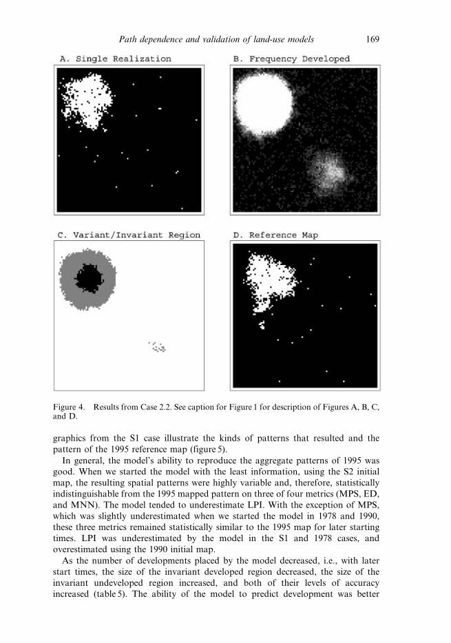
least partly (and in this case fully) captured by the model. Case 2.1 (figure 3) had no

invariant developed region and did no better than random at predicting the

locations of development within the variant region. Case 2.2 (figure 4), in which we

gave agents a new preference to be near the western edge of the map, did no better at

predicting the values of the landscape pattern statistics, i.e., except for MPS. Results

from both cases were not significantly different from the observed pattern metric

values. However, Case 2.2 performed better in terms of overall accuracy than did the

model that actually created the reference map (table 4). In addition, there was an

invariant region that was relatively accurately predicted, for both developed and

undeveloped regions.

Running the model for Washtenaw County produced results with varying degrees

of match to the 1995 development map (table 5). The user’s accuracy of the

development maps, averaged across model runs for each case, was generally low,

ranging from 3.5 to 18.6 percent, and decreasing with later starting times. The

Figure 2. Results from Case 1.3. See caption for figure 1 for description of figures A, B, C,and D.


Table 4. Results from second set of demonstrations. Results for Case 2.1 are from 31 runs ofthe model used to generate the reference map. Results from Case 2.2 are from 31 runs of themodel in which agents have an additional preference to be near the west edge.

Case 2.1 Case 2.2

Ave. % Dev Correct (std. dev.) 35.1 (33.6) 64.1 (6.1)Ref Map

LPI 7.5 7.4 (0.4) 7.2 (0.8)MPS 26.9 22.6 (3.0) 22.3 (3.5)ED 7.1 7.0 (0.4) 7.1 (0.7)MNN 575.6 549.6 (102.2) 527.7 (91.6)

ID (user’s acc.) 0 (na) 266 (94.0)IU (user’s acc.) 8006 (98.8) 8877 (99.0)C/R 4.433 8.092VC/VRD 0.954 0.936

Figure 3. Results from Case 2.1. See caption for figure 1 for description of figures A, B, C,and D.


graphics from the S1 case illustrate the kinds of patterns that resulted and the

pattern of the 1995 reference map (figure 5).

In general, the model’s ability to reproduce the aggregate patterns of 1995 was

good. When we started the model with the least information, using the S2 initial

map, the resulting spatial patterns were highly variable and, therefore, statistically

indistinguishable from the 1995 mapped pattern on three of four metrics (MPS, ED,

and MNN). The model tended to underestimate LPI. With the exception of MPS,

which was slightly underestimated when we started the model in 1978 and 1990,

these three metrics remained statistically similar to the 1995 map for later starting

times. LPI was underestimated by the model in the S1 and 1978 cases, and

overestimated using the 1990 initial map.

As the number of developments placed by the model decreased, i.e., with later

start times, the size of the invariant developed region decreased, the size of the

invariant undeveloped region increased, and both of their levels of accuracy

increased (table 5). The ability of the model to predict development was better

Figure 4. Results from Case 2.2. See caption for Figure 1 for description of Figures A, B, C,and D.


overall than in the invariant developed region, and improved relative to random at

later start times. The model, however, was never able to improve on random

location in the variant region, usually doing only half as well as random.

Table 5. Results from comparison of four Washtenaw County model runs with 1995 map ofdevelopment. Runs are identical except for the initial maps of development and the rates andnumbers of new residents and service centers (listed in table 2).

S2 S1 1978 1990

Ave. % Dev Correct(std. dev)

15.8 (1.43) 18.6 (1.22) 13.7 (0.40) 3.5 (0.40)

1995LPI 0.14 0.08 (0.07) 0.07 (0.03) 0.11 (0.04) 0.16 (0.03)MPS 4.9 4.3 (1.4) 5.2 (0.3) 4.8 (0.03) 4.8 (0.02)ED 30.1 27.9 (9.2) 29.9 (0.6) 30.2 (0.1) 30.1 (0.1)MNN 159.2 146.6 (48.1) 167.4 (4.1) 160.7 (0.9) 159.3 (0.7)

ID Size (user’s acc.) 934 (8.9) 1,526 (15.5) 5 (20.0) 0 (na)IU Size (user’s acc.) 120,827 (88.8) 135,809 (91.2) 156,690 (94.6) 162,102 (98.3)C/R 1.218 1.593 3.405 2.283VC/VRD 0.461 0.480 0.714 0.419

Figure 5. Results from Washtenaw County starting with the S1 map. See caption forfigure 1 for description of Figures A, B, C, and D.


6. Discussion and conclusions

In this paper, we have introduced the invariant-variant method to assess the

accuracy and variability of outcomes of spatial agent-based land-use models. This

method advances existing techniques that measure spatial similarity. Most

importantly, it helps us come to terms with a fundamental tension in land-use

modeling – the emphasis on accurate prediction of location and the recognition of

path dependence and stochastic uncertainty. The methods described here should

apply to any land-use models that have the potential to generate multiple outcomes.

They would not apply to models that are deterministic, and therefore make a single

prediction of settlement patterns. By definition, deterministic models cannot

generate path dependence unless one considers the impact of interventions. In that

case, our approach would be applicable with the invariant region being that portion

of the region that is developed regardless of the policy intervention.

Our proposed distinction between invariant and variant regions is a crude

measure, but one that allows researchers to better understand the processes that lead

to accurate (or inaccurate) predictions by their models. With it we can distinguish

between models that always get something right, and those that always get different

things right. And that difference matters. It may be possible to further develop the

statistical properties of the most useful of these and similar measures. Such measures

will enable us to categorize environments and actors who create systems for which

any accurate model will have low predictive accuracy and those who create systems

for which we should demand high accuracy.

We expect that, over time and by comparing across models, we can understand

what landscape attributes and behavioral characteristics lead to greater or lesser

predictability as captured by the relative size of the invariant region. For example,

homogeneity in the environment increases unpredictability because the number of

paths becomes unwieldy. Admittedly, size of the invariant region is not the only

possible measure of predictability, but it is a useful one. A large invariant region

suggests a predictable settlement pattern. A small invariant region implies that

history or even single events matter.

Our analysis emphasized path dependence as opposed to stochastic uncertainty

because of our interest, and that of many land-use modelers, in policy intervention.

Stochastic uncertainty, like the weather, is something we can all complain about but

not affect. Path dependence, at least in theory, offers the opportunity for

intervention. If we know that two paths of development patterns are possible, then

we might be able to influence the process, through policy and the use of what

Holland called ‘‘lever points,’’ such that the most desirable path, on some measure,

emerges (Holland 1995, Gladwell 2000). Path dependence makes fitting a model

more difficult and may tempt modelers to overfit the data, since often the one actual

path of development depends on specific details that influence the choices of early

settlers. On the other hand, path dependence creates the possibility of policy

leverage.

One lesson to be drawn from these simple models is the difficulty of obtaining a

good fit. When we used exactly the same model to generate and predict settlement

patterns, some of the cases (i.e., Cases 1.1 to 1.5 and Case 2.1) produced measures of

spatial similarity between the model results and the reference map that were not

good at all. Our models did not have many moving parts, and these limited degrees

of freedom provided only limited flexibility in the patterns they form. Nevertheless,

we cannot help but be struck by how poorly our models predict their own behavior,


even though there were clearly some predictable structures to the processes (i.e., they

were not simply random).

At the same time, the models do remarkably well at matching the aggregate

spatial patterns of the reference patterns, as measured by four selected spatial

pattern metrics. When we deliberately compared model output with a reference map

from a different model, as well as in the case of real data from Washtenaw County,

Michigan, the reference spatial pattern was usually statistically indistinguishable

from the model results. It is possible to imagine, of course, models in which the

aggregate pattern statistics would not agree well at all. However, the consistency of

the aggregate metrics in the cases presented here suggests that it is, indeed, much

easier to match the aggregate patterns than to match the locations of development.

In many modeling cases and for many applications, comparing aggregate statistics

will provide a sufficient test of the model and its response to particular

modifications. This is especially true when the question being investigated is

particularly concerned with the patterns in aggregate and not with locations of

development. In addition, as Parker and Meretsky (2004) have suggested, aggregate

pattern metrics might be useful to determine if the model is wrong (i.e., if the

aggregate patterns are not correct) even if it cannot validate that it is right.

The comparison between Cases 2.1 and 2.2 highlights the importance of

recognizing path dependence in land-use change processes and the dangers of

overfitting the model to data in the modeling processes. This danger, i.e., that the

model will match the outcome of a particular case well but misrepresent the process,

is endemic to land-use change models. Many models of land-use change are

developed through calibration and statistical fitting to observed changes, derived

from remotely sensed and GIS data sets. This rather extreme example makes the

point that, even though the outcomes of the model may match the reference map in

meaningful ways, e.g., both statistically and spatially, we cannot necessarily

conclude that the processes contained in the model are correct. If the processes are

not well represented, of course, then we possess limited ability to evaluate policy

outcomes, for example by changing incentives or creating zones that limit certain

activities on the landscape.

The results of running the model from multiple starting times in the history (and

pseudo-history) of Washtenaw County, Michigan, seem somewhat counterintuitive

at first, in that the overall match of the locations of newly settled agents with those

in the 1995 map decreased with increasing information (i.e., later starting times).

However, the additional metrics tell more of the story. The model actually improved

with later starting times when the matches were compared with the numbers that

would be expected at random. Fewer agents entering the landscape at the later times

means relatively more possible combinations of places they can locate in the

undeveloped part of the map. The model does reasonably well at predicting the

aggregate patterns, matching three of the four metrics, partially because much of

the aggregate pattern is predetermined in the initial maps. The fact that three of the

mean pattern-metric values were statistically indistinguishable from the 1995 values

when starting at even the earliest dates, however, suggests that the match is not only

due to the initial map information. The size of the invariant developed region

declined with later starting times, but became more accurate., When we located

fewer residents, we were much less likely to see them locate consistently, rightly or

wrongly. Further, within the variant region, the model located residents less well

than would be expected with simply random location. This suggests that some


features were missing or structurally wrong in our model. Two possibilities are that

our map of aesthetic quality in the outlying areas does not accurately reflect

preferences, or that soil qualities or some other willingness-to-sell characteristic of

locations contributes to where settlements occur.

In the context of the foregoing discussion, it is useful to reflect on how to proceed

with model development. If we use the results from Washtenaw County as an

indication of the validity of the model and wish to improve its validity, what should

be our next steps? There are a number of factors that we did not include in our

model that could be included in agent decision-making. These include the price of

land, zoning, the different kinds of residential, commercial, and industrial

developments, a different representation of roads and distances, and the presence

of areas restricted for development (like parks). Any of these factors could be

included in the model in a way that would improve the fit of the output to the 1995

map. But, each new factor we add will have associated with it parameters that need

to be set. As soon as we start fitting these parameters according to the values that

produce outputs that best fit the data, we run the risk of losing control of the

process-based understanding that models of this sort helps us grapple with. As we

proceed, the question becomes: are we interested in fitting the data or understanding

the process?

Acknowledgements

For this work, we benefited from financial support from the National Science

Foundation Biocomplexity in the Environment program (BCS-0119804) and

computational resources from the Center for the Study of Complex Systems at

the University of Michigan.

ReferencesANDERSSON, C., LINDGREN, K., RASMUSSEN, S. and WHITE, R., 2002, Urban growth

simulation from ‘‘first principles.’’ Physical Review E, 66, (026204).

ARTHUR, W.B., 1988, Urban systems and historical path dependence. In Cities and Their Vital

Systems, J.H. Ausubel and R. Herman (Eds.), pp. 85–97 (Washington, DC: National

Academy Press).

ARTHUR, W.B., 1989, Competing technologies, increasing returns and lock-in by historical

events. The Economic Journal, 99, pp. 116–131.

ATKINSON, G. and OLESON, T., 1996, Urban sprawl as a path dependent process. Journal of

Economic Issues, 30, pp. 609–615.

BALMANN, A., 2001, Modeling land use with multi-agent systems: Perspectives for the analysis

of agricultural policies. In Proceedings, IIFET Conference Microbehavior and

Macroresults (Corvallis: Oregon State University).

BATTY, M. and XIE, Y., 1994, From cells to cities. Environment and Planning B, 21,

pp. S31–S48.

BATTY, M. and LONGLEY, P., 1994, Fractal Cities (San Diego: Academic Press).

CLARKE, K.C., GAYDOS, L. and HOPPEN, S., 1996, A self-modifying cellular automaton model

of historical urbanization in the San Francisco Bay area. Environment and Planning B,

24, pp. 247–261.

COHEN, J., 1960, A coefficient of agreement for nominal scales. Educational and Psychological

Measurement, 20, pp. 37–46.

CONGALTON, R.G., 1991, A review of assessing the accuracy of classifications of remotely

sensed data. Remote Sensing of Environment, 37, pp. 35–46.

COSTANZA, R., 1989, Model goodness of fit: a multiple resolution procedure. Ecological

Modelling, 47, pp. 199–215.


DOSI, G., 1984, Technical Change and Industrial Transformation (London: Macmillan).

GLADWELL, M., 2000, The Tipping Point: How Little Things Can Make a Big Difference

(Boston: Little Brown).

HAGEN, A., 2003, Fuzzy set approach to assessing similarity of categorical maps. International

Journal of Geographical Information Science, 17, pp. 235–249.

HOLLAND, J.H., 1995, Hidden Order: How Adaptation Builds Complexity (Reading, Mass.:

Addison-Wesley).

IRWIN, E.G. and GEOGHEGAN, J., 2001, Theory, data, methods: developing spatially explicit

economic models of land use change. Agriculture, Ecosystems and Environment, 85,

pp. 7–23.

KOK, K., FARROW, A., VELDKAMP, A. and VERBURG, P.H., 2001, A method and application

of multi-scale validation in spatial land use models. Agriculture, Ecosystems and

Environment, 85, pp. 223–238.

MAKSE, H.A., DE ANDRADE, J.S., BATTY, M., SHLOMO, H. and STANLEY, H.E., 1998,

Modelling urban growth patterns with correlated percolation. Physical Review E, 58,

pp. 7054–62.

MCGARIGAL, K. and MARKS, B.J., 1995, FRAGSTATS: Spatial Pattern Analysis Program for

Quantifying Landscape Structure, General Technical Report PNW-GTR-

351 (Portland, OR: USDA Forest Service, Pacific Northwest Research Station).

PAHL-WOSTL, C., 1995, The Dynamic Natural of Ecosystems: Chaos and Order Entwined

(Chichester: John Wiley).

PARKER, D. and MERETSKY, V., 2004, Measuring pattern outcomes in an agent based model

of edge-effect externalities using spatial metrics. Agriculture Ecosystems and

Environment, 101, pp. 233–250.

PONTIUS, R.G., 2000, Quantification error versus location error in comparison of categorical

maps. Photogrammetric Engineering & Remote Sensing, 66, pp. 1011–1016.

PONTIUS, R.G., 2002, Statistical methods to partition effects of quantity and location during

comparison of categorical maps at multiple resolutions. Photogrammetric Engineering

& Remote Sensing, 68, pp. 1041–1049.

RAND, W., BROWN, D.G., PAGE, S.E., RIOLO, R., FERNANDEZ, L.E. and ZELLNER, M., 2003,

Statistical validation of spatial patterns in agent-based models. In Proceedings of

Agent Based Simulation 2003, Montpellier, France.

RAND, W., ZELLNER, M., PAGE, S.E., RIOLO, R., BROWN, D.G. and FERNANDEZ, L.E., 2002,

The complex interaction of agents and environments: An example in urban sprawl. In

Proceedings of Agent 2002, Social Agents: Ecology, Exchange and Evolution, Chicago,

IL.

TURNER, M.G., GARDNER, R.H. and O’NEILL, R.V., 2001, Landscape Ecology in Theory and

Practice: Pattern and Process (New York: Springer-Verlag).

WHITE, R. and ENGELEN, G., 1997, Cellular automata as the basis of integrated dynamic

regional modeling. Environment and Planning B, 24, pp. 235–246.

WILSON, A.G., 2000, Complex Spatial Systems: The Modelling Foundations of Urban and

Regional Analysis (New York: Pearson).

174 Path dependence and validation of land-use models

Path dependence and the validation of agent-based spatial ... · 2. An agent-based model of land...

Documents

Transcript of Path dependence and the validation of agent-based spatial ... · 2. An agent-based model of land...