Paternity leave and the motherhood Penalty: new causal ... · This paper contributes to the...

signe hald andersen

study paper 114 november 2016

The Research UnitSølvgade 10, 2nd floor1307 Copenhagen, Denmark

Danmarks StatistikSejrøgade 112100 Copenhagen, DenmarkISSN 0908-3979

Paternity leave and the motherhood Penalty: new causal evidence

The Rockwool Foundation Research Unit

Study Paper No. 114

Paternity leave and the motherhood Penalty: new causal evidence

Signe Hald Andersen

Copenhagen 2016

Paternity leave and the motherhood penalty: New causal evidence

Study Paper No. 114

Published by:© The Rockwool Foundation Research Unit

Address:The Rockwool Foundation Research UnitSoelvgade 10, 2.tv.DK-1307 Copenhagen K

Telephone +45 33 34 48 00E-mail [email protected] site: www.en.rff.dk

November 2016

1 1

Paternity leave and the motherhood penalty: New causal evidence

Signe Hald Andersen

Abstract

This paper contributes to the literature on the penalty of motherhood and maternity leave by analyzing

whether father’s relative share of the total parental leave taken when a child is born affects mother’s post-

leave labor market performance. For this purpose, I use full sample, administrative data from Statistics

Denmark and facilitate causal inference by exploiting five reforms of the parental leave. Results show that

father’s involvement in the childcare benefits mother’s labor market outcomes in both the short and longer

run.

3 2

Introduction

Numerous studies document a significant penalty of motherhood on labor market outcomes, across

socioeconomic groups (e.g. Budig & Hodges, 2010; Evertsson & Duvander, 2010) and institutional contexts

(as documented in e.g. Gangl & Ziefle, 2009; Aisenbrey et al, 2009). According to researchers, the

motherhood penalty reflects the statistical discrimination of mothers at the labor market, the human capital

depreciation caused by time spent away from the labor market, etc. (Staff & Mortimer, 2012). Yet, staying at

home, taking care of one’s children may not only cause a reduction in labor market relevant human capital,

but also increase one’s domestic human capital. This is the specialization hypothesis as implied by Becker’s

theory on human capital and the family (Becker, 1981; see Bonke et al (2004) for empirical support).

Accumulating such domestic capital is, however, likely to reinforce the negative effects of motherhood on

subsequent labor market performance, by giving mothers a comparative advantage over fathers when e.g.

during illness, children need extra care or when other domestic areas require increased attention. The same

process is likely to give fathers a comparative advantage at the labor market, thus increasing his wages

relative to the mother and hereby his economic power in the household. The father may use this power to

avoid household work, to the extent that this is a less valued activity. In sum, maternity leave may increase

the likelihood that compared to fathers, mothers attend to domestic chores even post-leave, and that mothers

hereby experience additional absence from the labor market, resulting in even further human capital

depreciation (as also noted by Ekberg et al, 2005).

A number of countries now offer paid, ear-marked leave for fathers (e.g. the daddy quota in Sweden, Norway

and Iceland), just as many countries allow the parents to share a given number of weeks of paid leave. These

options for leave enable the father to also gain domestic capital, and may inspire a more equal distribution of

household tasks between fathers and mothers also after all parental leave has ended. Thus, with fathers’

gaining more insight into the workings of the household he will enter – and will be expected to enter – more

forcefully into the negotiations on household matters. And since his leave will allow the mother to have a

stronger commitment to the labor market, it will also improve her position in labor market related

negotiations in the household (e.g. on who should stay home from work in case of sick children). While

4 3

causal studies on this topic are limited, we now know that father’s increased use of leave facilitates a more

equal division of labor in the household (see Kotsadam & Finseraas, 2011; Patnaik, 2014). This suggests that

the motherhood penalty does not only reflect the duration of mother’s own leave, but also of that of the

father of her child: The longer his leave is relative to her’s, the more likely it is that he also attends to

domestic matters, thus reducing the mother’s post leave absence from the labor market.

A small group of studies analyses how father’s leave impacts mother’s labor market outcomes. But while e.g.

Johannsson (2010) use Swedish data to show a positive effect of father’s leave on mother’s earnings (even if

effects vary by model specification), Cools et al. (2011) find evidence of a negative effect on Norwegian

data. Also, evidence from Estonia and Denmark points to no correlation between father’s leave and mother’s

labor market outcomes (Karu, 2012; Pylkkänen & Smith, 2003) just as there is evidence from Sweden that

father’s leave does not reduce mother’s sickness absence (Ugreninov, 2013). Importantly though, none of

these studies consider father’s leave relative to mother’s leave, but instead look at the absolute length of

father’s leave. However, if part of the motherhood penalty reflects mother’s comparative advantage over the

father in household chores and her comparative disadvantage at the labor market, focusing on fathers’ leave

in days or months provide us with only half the information that we need. Thus to understand if the

introduction of a daddy quota or other changes in rules regarding parental leave affect the motherhood

penalty, by changing the power balance in the intra household negotiations, we need to focus on measures

reflecting fathers’ take up of paternity leave relative to mothers’ take up of maternity leave.

My study is the first to take that route and test whether father’s leave relative to mother’s leave has a causal

effect on mother’s subsequent labor market outcomes. For this purpose, I use full sample, administrative data

from Statistics Denmark and facilitate causal inference by exploiting five reforms of the parental leave.

Results show that when fathers’ share of the leave increases – either because the duration of his leave

increases or because the duration of mothers leave decreases – it causally reduces the labor market penalty of

maternity leave.

5 4

The motherhood penalty

The literature offers a range of explanations why motherhood affects women’s labor market outcomes. Sigle-

Ruston & Waldfogel (2007) summarizes the literature and argue that existing explanations fall into four

categories, which are not necessarily mutually exclusive. The first explanation draws on human capital

theory and describes how motherhood reduces women’s investments at the labor market – not only does the

woman take leave for shorter or longer periods at the time of the child’s birth, having a child also increases

the likelihood that she works part-time. Both elements reduce mothers’ work experience and job tenure

compared to non-mothers and to men, and this reduction in human capital will affect labor market outcomes

negatively (for empirical support, see Lundberg & Rose, 2000; Kahn et al 2014). The second explanation is

related and concerns the type of job arrangements mothers negotiate to make their work life compatible with

their family life. To secure flexibility, mothers may trade wages and fulltime work for flexibility, or

competitive high paid private sector jobs for more family friendly, but lower paid public sector jobs (as

found by Pertold-Gebick et al, 2016). Such arrangements may reduce both their human capital and labor

market outcomes.

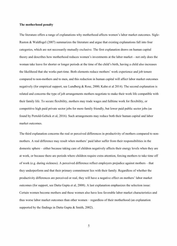
The third explanation concerns the real or perceived differences in productivity of mothers compared to non-

mothers. A real difference may result when mothers’ paid labor suffer from their responsibilities in the

domestic sphere – either because taking care of children negatively affects their energy levels when they are

at work, or because there are periods where children require extra attention, forcing mothers to take time off

of work (e.g. during sickness). A perceived difference reflect employers prejudice against mothers – that

they underperform and that their primary commitment lies with their family. Regardless of whether the

productivity differences are perceived or real, they will have a negative effect on mothers’ labor market

outcomes (for support, see Datta Gupta et al, 2008). A last explanation emphasizes the selection issue:

Certain women become mothers and these women also have less favorable labor market characteristics and

thus worse labor market outcomes than other women – regardless of their motherhood (an explanation

supported by the findings in Datta Gupta & Smith, 2002).

6 5

Given this plethora of explanations of the relationship between motherhood and labor market outcomes, all

pointing to problems pertaining to mothers’ actual and expected responsibilities in the household, there is an

evident need for understanding the implications of policies that encourage fathers to take larger

responsibilities in caring for children and improve his relative position in household decisions.

The implications of paternity leave

Given these four explanations of the motherhood penalty there are at least two routes through which father’s

leave may matter. First, to the extent that the duration of father’s and mother’s leave is negatively correlated,

e.g. because policies allow parents to share a given number of weeks, father’s longer leave will reduce the

amount time that mother spend away from the labor market and reduce the depreciation of her labor market

capital. In addition, parallel to the effect of mother’s leave on her labor market capital, we may also expect

father’s time away from work due to leave to affect his labor market capital (a matter that is still disputed,

though, see Cools et al, 2011; Johannsson, 2019; Rege & Solli, 2013). Thus the overall bargaining situation

in the household changes to the mother’s advantage; not only does her labor market capital suffer less, his

capital suffers more, even if it is likely that he still has more labor market capital, overall. This advantage is

likely to also have an effect on mother’s subsequent labor market outcomes, because it will legitimize her

stronger involvement at the labor market.

Second, father’s leave may also affect mother’s real or perceived productivity loss. Since father’s leave

increases his household capital, it also increases the probability that parents share domestic responsibilities,

by simultaneously giving him more say in household matters and her more legitimacy in counting on his

participation in taking care of chores. This will free some of the mother’s resources and positively affect her

productivity. Furthermore, the father’s leave is a strong signal to the mother’s employer of such shared

responsibility in her household, a signal which may counteract the employer’s expectations of the mother’s

lowered productivity (Schober, 2014).

In sum, we have valid reasons to expect father’s leave to affect the motherhood penalty, and this expectation

rests on how father’s leave interferes with parents’ internal balance of domestic capital and labor market

7 6

capital. This then emphasizes the importance of focusing the father’s relative share of the total parental

leave, rather than just the number of days or months that fathers take leave.

Selection issues

When considering household dynamics, we cannot, however, disregard issues pertaining to the selection of

specific women into motherhood (the fourth explanation of the motherhood penalty presented above), or for

that matter, the fact that it is likely to be specific types of fathers that appreciate and take advantage of the

opportunities for paternity leave. This means that if we observe better labor market outcomes for mothers

whose partners take long leave it may simply be an indication that such couples are already committed to

egalitarian principles and that the duration of father’s leave – and his relative share of the total leave - is a

symptom of this commitment, rather than the actual cause of the mother’s subsequent labor market

outcomes.

Existing literature widely acknowledges such problems of selection and solves them through various routes,

of which the predominant strategies involve the implementation of fixed effects methods (Johannsson, 2010;

Gangl & Ziefle, 2009) and the use of policy reforms in regression discontinuity designs (Lalive et al, 2011),

and difference- in-differences models (Cools et al., 2011; Johannsson, 2010; Rege & Solli, 2013). My study

follows this tradition and use five reforms of the parental leave system as instruments in standard IV-models

(estimated as two stage least squares models).

Equation 1 and 2 show the model

𝑓𝑓𝑓𝑓𝑓𝑓ℎ𝑒𝑒𝑟𝑟′𝑠𝑠 𝑠𝑠ℎ𝑓𝑓𝑟𝑟𝑒𝑒 𝑜𝑜𝑓𝑓 𝑓𝑓𝑜𝑜𝑓𝑓𝑓𝑓𝑡𝑡 𝑡𝑡𝑒𝑒𝑓𝑓𝑙𝑙𝑒𝑒ℎ = 𝛼𝛼ℎ + 𝛿𝛿1𝑥𝑥ℎ + 𝜃𝜃𝑟𝑟𝑒𝑒𝑓𝑓𝑜𝑜𝑟𝑟𝑟𝑟ℎ + 𝑟𝑟ℎ [1]

𝑟𝑟𝑜𝑜𝑓𝑓ℎ𝑒𝑒𝑟𝑟′𝑠𝑠𝑡𝑡𝑓𝑓𝑠𝑠𝑜𝑜𝑟𝑟 𝑟𝑟𝑓𝑓𝑟𝑟𝑚𝑚𝑒𝑒𝑓𝑓 𝑜𝑜𝑜𝑜𝑓𝑓𝑜𝑜𝑜𝑜𝑟𝑟𝑒𝑒𝑠𝑠ℎ = 𝛼𝛼2 + 𝛿𝛿2𝑥𝑥ℎ + 𝛽𝛽𝑓𝑓𝑓𝑓𝑓𝑓ℎ𝑒𝑒𝑟𝑟′𝑠𝑠 𝑠𝑠ℎ𝑓𝑓𝑟𝑟𝑒𝑒 𝑜𝑜𝑓𝑓 𝑓𝑓𝑜𝑜𝑓𝑓𝑓𝑓𝑡𝑡 𝑡𝑡𝑒𝑒𝑓𝑓𝑙𝑙𝑒𝑒� ℎ + 𝑜𝑜ℎ [2]

In both equations, h is the household (h=1,…N). Equation 1 is the first stage equation, in

which the endogenous variable (father’s share of total leave) is regressed on the vector of exogenous

household controls xh and the instrument. The second stage uses the predicted (rather than the actual) value

8 7

of the endogenous variable to predict the outcome variable, mother’s labor market outcomes, along with the

vector of controls, xh. The standard errors in the second stage are adjusted to account for the fact that we use

the predicted value of the endogenous variable. Random error terms are rh and uh. If the instrument is valid,

there is no correlation between the predicted value of the endogenous variable and the error term in the

second stage equation, and the model will produce consistent, plausibly causal, results.

Parental leave in Denmark

As in most countries, the parental leave system in Denmark has changed and become more generous over

time. The Danish Factory Act from 1901 was the first to stipulate mother’s rights at childbirth, and it granted

female factory workers the right to 4 weeks of leave (starting from the time of birth).1 Women with few

economic resources could get a small financial compensation during the four weeks.

Since then, parental leave in Denmark has undergone very significant changes, and today, Danish parents are

entitled to 52 weeks of leave in total, of which 4 respectively 14 are earmarked for mothers immediately

before respectively after the child birth, 2 are earmarked for fathers and parents may share the remaining 32

weeks as they wish. However, between 1980 and now, there have been 4 substantial changes – April 1989,

July 1997, March 1998, March 2002 - that I will use as instruments in my IV model. These four significant

changes concern two important aspects of the leave, namely the extent of earmarked leave for fathers (the

1998 and 2002 reforms) and wage compensation during the leave (the 1989 and 1997 reforms). The

importance of the 1998 and 2002 reforms for my study are quite straightforward as they aim at changing

father’s leave relative to mother’s – the 1998 reform is likely to increase father’s share relative to mother’s

and the 2002 reform will most likely reduce father’s share. But also the two earlier reforms that change the

financial incentives of taking leave are relevant, since they address one of the major concerns in a lot of

families; fathers are often the main breadwinner in most families, which makes it difficult for families to

1 Only women employed at factories with more than 4 employees were granted this right

9 8

afford his prolonged leave. However the introduction of wage compensation during the leave removes this

obstacle.

Importantly though, the wage compensation introduced with the 1989 and 1997 reforms also

changes mothers’ financial incentives of taking leave. Thus, using these reforms, a change in father’s share

of the total leave may arise from a change in both the number of days or weeks that the father is on leave and

a change in the number of days and weeks that the mother is on leave. This is a potential threat to the causal

interpretation of my results, as there might be a correlation between father’s relative share of the total leave

and the total leave taken in the family, such that e.g. father’s share may be larger when the total leave is

shorter and vice versa. In such cases father’s share of the total leave also captures the length of mother’s

actual leave, something which may affect her labor market outcomes directly. The coefficient I estimate in

the IV-model would then not only represent the causal effect of his share, but also of her absolute leave.

While both elements represent the reform effect, the interpretation is less clear, and in particular, we will not

be able to answer the research question of the importance of father’s share of the total leave. Thus, to

separate out these two reform effects, my model include an indicator of the total number of days of leave

taken by the parents. However, as the total leave taken by the parents is also a choice variable – and thus

likely to be endogenous to mothers’ labor market outcomes – including this indicator in the models may

introduce bias, also in the assumed causal effect of my endogenous and instrumented variable, depending on

the size of the correlation between the two parameters. To assess the size and the importance of this potential

problem, I present results both with and without controlling for total leave.

The 1994 labor market reform

When considering parental leave in a Danish context we need to also take into account the

labor market reform that was announced June 30th 1993 and implemented January 1st 1994. Among others,

this reform introduced a new type of leave, the so-called child care leave. The leave targeted not only parents

of new born babies, but all parents with children below the age of 9, and granted them the right to a

minimum of 13 and a maximum of 36 weeks of paid leave (the compensation equaled 80 percent of

10 9

unemployment insurance benefits). At this point in time the duration of the traditional leave was 32 weeks (8

weeks before the birth and 24 weeks after) and with this new addition parents now had the right to a total of

68 weeks of leave (of which 10 of the 24 weeks and all the additional 13-36 weeks could be shared freely

between the parents). Subsequent reforms changed the scheme several times throughout the 1990s. Studies

show that the take up rate among women was high, and, as could be expected, low among men (Olsen,

2000).

While the child care leave had the primary purpose of reducing friction at the labor market

and hereby counteracting the rising unemployment rates in the 90’s, it is likely to also have affected the ratio

between parents’ child related leave, by increasing the availability of paid leave. This means that I now have

an additional reform that I may use as a fifth instrument in my analysis, but also that I need to consider if and

how to include this type of leave in the other analyses: Clearly, the 1989-reform is too early in time to be

influenced by the child care leave, and the changes laid out with the 1997- reform concerns only the actual

parental leave. However, the 1998-reform may shift some fathers from child care leave to parental leave,

which means that we should consider both systems together for this reform. Also, one of the purposes of the

2002-reform was to simplify the leave system, and offer parents just one type of leave, parental leave. This

means that the changes laid out in this reform do not only reflect a political reformation of the parental leave

system, but the attempt to combine the child care leave scheme with the parental leave scheme. In sum, if my

measure of leave in the 1998 and 2002-analyses then only includes actual parental leave and not also the

leave taken under the child care scheme, it will look as if the reform causes an increase in the number of

weeks available for parental leave, when in fact what is going on, is a re-categorization of weeks available

for child care leave into weeks available for parental leave. Hence a true reflection of the effect of the 1998-

and the 2002-reforms requires that the measurement of leave used in the analyses relying on these reforms

for causal inferences should include both parental leave and child care leave. Similarly, the specification

relying on the 1994-reform should also include both types of leave. I elaborate on this issue in the data

section.

11 10

Table 1 below lays out the content of the reforms.

Table 1: The five reforms

Reform date (announcement date)

Who did it affect?

Content Post birth leave after the reform

Policy implication for fathers

April 1989 Public sector employees

Full wage compensation during the 32 weeks of leave. 22 weeks earmarked for mothers and 10 weeks sharable between parents

14 w for mother, 10 w sharable

Increased economic incentive for fathers to take leave

January 1994 (June 1993)

All parents of children below age 9

13-36 additional weeks of paid leave (80 percent of unemployment insurance benefits)

14 w for mother, 10 w sharable + 36 w of child care leave

Increased economic incentives for parents to take leave

March 1997 (March 1995)

Private sector employees

Full wage compensation during leave. 14 weeks earmarked for mothers and 2 weeks earmarked for fathers

14 w for mother, 10 w sharable + 36 w of child care leave

Increased economic incentives for parents to take leave

April1998 (April 3rd, 1998)

All fathers, children born after October 15th, 1997

2 more weeks earmarked for fathers – a total of 4 weeks earmarked for fathers

14 w for mother, 4 w for father, 8 w sharable + 36 w of child care leave

Increased non-monetary incentive for father to take leave

March 2002 (March 25th, 2002)

All families, children born after January 1st 2002

No. of weeks earmarked for fathers reduced to 2, but no. of sharable weeks increased to 32

14 w for mother, 2 w for father, 32 w sharable

Reduced non-monetary incentive for father to take leave

Figure 1 shows the average days of leave taken by first time mothers respectively fathers, by

the child’s birth month from January 1985 to December 2003. As shown, especially the duration of mother’s

leave increases over time – from an average of a little more than 160 days to a little more than 250 days –

and we see some discrete jumps in the duration at January 1994, which marks the implementation of the

parental leave reform, and in 2002 at the time of the implementation of the new, prolonged leave scheme.

Interestingly – and unexpectedly – mothers also appear to respond to the 1998-reform by taking up more

child care leave, even if this reform only targets men. This could be an indication that mothers did not wish

to reduce their total leave as a result of “losing” 2 of the sharable 10 weeks to the fathers, and that they then

used 2 more weeks of child care leave as compensation.

The duration of father’s leave also increases during this period, however far less. At the

beginning of the period fathers take approximately 7 days of leave and at the end of the period, fathers’ leave

has increased to a little more than 14 days on average. For fathers, the biggest increase seems to happen with

12 11

the implementation of the parental leave scheme in 1994, just as there is a small increase from 1998 to 1999.

The effect of the additional reforms seems less evident.

Figure 1: Leave by birth month. First time mothers and fathers

Importantly though, we cannot expect the reform in 1989 and 1997 which introduces wage compensation

during leave to affect all men equally; the first reform concerns only public sector employees and the second

reform concerns only private sector employees. Hence, figure 2 shows the average duration of leave taken by

men employed in the private respectively the public sector at the time of their child’s birth from 1985 to

2003. The figure not only demonstrates an expected higher take-up rate of men employed in the public

sector, it also shows how the reform effects differ by sector. Whereas men employed in the public sector

respond to the 1989 reform by increasing the average duration of their leave from April 1989 onwards, there

is no action at this point in time for privately employed men. We also see how the implementation of

parental leave in 1994 increases the duration of leave taken by publicly employed men, and even if this

reform also targets the privately employed men, they do not seem to respond to it. And while there is no

clear response to the 1997 reform which introduces full wage compensation in the private sector (for neither

group of men), we see a non-negligible increase in the duration of leave taken by men employed in both

0

50

100

150

200

250

300

jan-

86

nov-

86

sep-

87

jul-8

8

maj

-89

mar

-90

jan-

91

nov-

91

sep-

92

jul-9

3

maj

-94

mar

-95

jan-

96

nov-

96

sep-

97

jul-9

8

maj

-99

mar

-00

jan-

01

nov-

01

sep-

02

jul-0

3

maj

-04

Mother: p + cc leave Mother: p leave

Father: p + cc leave Father: p leave

12

sectors with the introduction of earmarked leave in 1998. The last reform considered here – the 2002 reform

which increases the total number of weeks of leave, but reduces the number of weeks earmarked for fathers –

appears to increase the duration of both parental leave and child care leave in private sectors and child care

leave in the public section, but reduce parental leave in the public sector.

Figure 2: Leave by birth month. Fathers, by sector

In sum, the combined information gained from figures 1 and 2, is that we may use the five reforms as

sources of exogenous variation in the duration of father’s leave and hence as exogenous variation in the ratio

between parents leave.

Problems pertaining to time trends

A key assumption when using IV-models is that the instrument only affects the outcome through the

endogenous regressor – this is the untestable exclusion restriction. However because my instrument is a date

in time, I face the risk that (estimated) differences on outcome measures between families affected by the

0

10

20

30

40

50

60

70

80

90

jan-

86ok

t-86

jul-8

7ap

r-88

jan-

89ok

t-89

jul-9

0ap

r-91

jan-

92ok

t-92

jul-9

3ap

r-94

jan-

95ok

t-95

jul-9

6ap

r-97

jan-

98ok

t-98

jul-9

9ap

r-00

jan-

01ok

t-01

jul-0

2ap

r-03

jan-

04ok

t-04

father, public sector: p +cc father, public sector: p

Father, privat: p + cc Father, privat: p

13 12

sectors with the introduction of earmarked leave in 1998. The last reform considered here – the 2002 reform

which increases the total number of weeks of leave, but reduces the number of weeks earmarked for fathers –

appears to increase the duration of both parental leave and child care leave in private sectors and child care

leave in the public section, but reduce parental leave in the public sector.

Figure 2: Leave by birth month. Fathers, by sector

In sum, the combined information gained from figures 1 and 2, is that we may use the five reforms as

sources of exogenous variation in the duration of father’s leave and hence as exogenous variation in the ratio

between parents leave.

Problems pertaining to time trends

A key assumption when using IV-models is that the instrument only affects the outcome through the

endogenous regressor – this is the untestable exclusion restriction. However because my instrument is a date

in time, I face the risk that (estimated) differences on outcome measures between families affected by the

0

10

20

30

40

50

60

70

80

90

jan-

86ok

t-86

jul-8

7ap

r-88

jan-

89ok

t-89

jul-9

0ap

r-91

jan-

92ok

t-92

jul-9

3ap

r-94

jan-

95ok

t-95

jul-9

6ap

r-97

jan-

98ok

t-98

jul-9

9ap

r-00

jan-

01ok

t-01

jul-0

2ap

r-03

jan-

04ok

t-04

father, public sector: p +cc father, public sector: p

Father, privat: p + cc Father, privat: p

14 14

Figure 4:Age first childbirth, mothers and fathers,

All this implies that before-/after-reform samples may differ on various characteristics, which may be

indicators that the instrument does not fulfill the exclusion restriction.

I address these possible threats to the exclusion restriction through two routes. First, rather than using my IV-

setup on the immediately available before- and after samples, I use matched before-after samples. This is to

ensure that these two samples are directly comparable on all relevant observed characteristics, and that

differences in age at parenthood – and the resulting differences in life situations - between them do not drive

my results. Second, rather than using raw labor market indicators, I use indexed versions, to ensure that

changes over years – and thus differences between the before and after groups - do not just reflect general

time trends in favor of one of the two groups. This is similar to the standard praxis of deflating income to an

index year.

0

5

10

15

20

25

30

35

1986 1988 1990 1992 1994 1996 1998 2000 2002 2004 2006 2008 2010 2012 2014

Age

at fi

rst c

hild

birt

h

First time mothers First time fathers

13

reforms (who give birth after the reform) and families unaffected by the reform (who give birth before the

reform) reflect more general time trends - rather than the reform effect – simply because my date-in-time

instrument is correlated with time trends in my outcome measures. In fact, during the time period covered by

my 5 reforms, we see a) variation in labor market outcomes that are caused by the business cycle (as

illustrated in figure 3 below using female unemployment rates) and b) increased age at family formation

which implies that over time, families are likely to have a stronger foothold at the labor market at the time

that they start producing children.

Figure 3: Women’s unemployment rates, 1979-2015

0

2

4

6

8

10

12

14

1986

1987

1988

1989

1990

1991

1992

1993

1994

1995

1996

1997

1998

1999

2000

2001

2002

2003

2004

2005

2006

2007

2008

2009

2010

2011

2012

2013

2014

2015

Une

mpl

oym

ent r

ate

in p

erce

ntag

es

unemployed women as share of female labor force

15 14

Figure 4:Age first childbirth, mothers and fathers,

All this implies that before-/after-reform samples may differ on various characteristics, which may be

indicators that the instrument does not fulfill the exclusion restriction.

I address these possible threats to the exclusion restriction through two routes. First, rather than using my IV-

setup on the immediately available before- and after samples, I use matched before-after samples. This is to

ensure that these two samples are directly comparable on all relevant observed characteristics, and that

differences in age at parenthood – and the resulting differences in life situations - between them do not drive

my results. Second, rather than using raw labor market indicators, I use indexed versions, to ensure that

changes over years – and thus differences between the before and after groups - do not just reflect general

time trends in favor of one of the two groups. This is similar to the standard praxis of deflating income to an

index year.

0

5

10

15

20

25

30

35

1986 1988 1990 1992 1994 1996 1998 2000 2002 2004 2006 2008 2010 2012 2014

Age

at fi

rst c

hild

birt

h

First time mothers First time fathers

16 15

Data

To study the effect of father’s relative share of the total leave on mother’s labor market outcomes I

rely on administrative data from Statistics Denmark. All residents in Denmark have a unique personal

identification number (similar to the social security number in the US) that is used to identify the residents in

all major transactions with public authorities as well as in transactions with a range of private institutions as

e.g. banks. Statistics Denmark collects an extensive part of the information registered by this unique personal

identification number, and makes these data available for statistical and research purposes. These registers

are available as a yearly panel dating back from 1980 and they contain information on dealings with the

welfare system, including parental leave, childbirth, marital status and partner ID.

The Danish administrative registers are well suited for the study that I undertake in this paper,

because the registers allow me to link parents of a child, and because we observe the labor markets histories

of both parts, as well as a range of other characteristics.

As described above, my identification strategy relies on the implementation of five different reforms,

which I use in five different IV-regression models based on samples including households with child births

happening from one year before till one year after the reform. I use this 2 year window to prevent seasonal

variation in who gives birth when from influencing my results. Given the target groups of these reforms

models relying on the 1989 and 1997 reforms for identification of causal effect, only rests on data from

households in which the male part is publicly respectively privately employed.

I use only first births to avoid interference from previous parental leave, and to hereby simplify the

model, and I exclude single headed households. I choose not to use another obvious strategy where I include

all five instruments in one model which would then cover the long time span from before 1989 till after

2002; with such a long time span, quite a few other macro level changes and time trends will have affected

both labor market and family policies, and the causal interpretation results based on such a model will be less

straightforward.

16

Matched samples

As described above, to secure comparable before and after groups, my analyses relies on matched

rather than full samples. For this purpose I conduct a 1-to-1 matching based on an estimated propensity

score, of families who have children before the reform with families who have children after the reform.

To estimate the propensity score I use a range of standard control variables, which are all key

indicators of the families’ life situation and labor market affiliation. The group of control variables include

mother’s age and marital status at child birth, mother’s and father’s unemployment and income the year

before the childbirth (varying between 0 and 10, with 0 indicating no unemployment during the year and 10

indicating full unemployment during the year), and last, mother’s and father’s educational level. Table 3

below shows the post-matching descriptive statistics for before and after samples (including t-values for

differences in means), with matching test statistics (R2 and χ2) presented at the bottom of the table. As

demonstrated, the matching has been largely successful with almost perfectly balanced before and after

samples, except for the 1994-reform, where father’s income could not be completely balanced.

Table 3: Descriptive statistics by reform

1989 1994 1997 1998 2002 . Controls Treated Controls Treated Controls Treated Controls Treated Controls Treated mean/sd mean/sd mean/sd mean/sd mean/sd mean/sd mean/sd mean/sd mean/sd mean/sd Outcome variables Mother’s unem. t+2

0.68 0.72 0.73 0.87*** 0.80 0.82 0.81 0.80 0.78 0.84** (1.30) (1.29) (1.25) (1.50) (1.60) (1.72) (1.73) (1.77) (1.71) (1.75)

Mother’s unem. t+3

0.61 0.65 0.76 0.77 0.70 0.71 0.70 0.70 0.70 0.73 (1.20) (1.18) (1.41) (1.48) (1.59) (1.64) (1.65) (1.68) (1.60) (1.71)


0.56 0.58 0.75 0.73 0.70 0.71 0.71 0.71 0.75 0.80** (1.10) (1.11) (1.48) (1.53) (1.67) (1.70) (1.73) (1.73) (1.76) (2.03)

Mother’s wages t+2 (100,000 DKK)

1.61 1.59 1.32 1.38*** 1.62 1.62 1.59 1.62 1.67 1.67 (0.97) (1.00) (1.06) (1.06) (1.07) (1.07) (1.10) (1.16) (1.19) (1.21)


1.64 1.61 1.35 1.42*** 1.63 1.63 1.61 1.62* 1.64 1.64 (0.99) (1.04) (1.06) (1.06) (1.07) (1.09) (1.12) (1.13) (1.19) (1.20)


1.69 1.62** 1.45 1.52*** 1.70 1.70 1.69 1.66* 1.73 1.77** (1.01) (1.05) (1.06) (1.07) (1.09) (1.11) (1.14) (1.16) (1.21) (1.23)

1715

Data

To study the effect of father’s relative share of the total leave on mother’s labor market outcomes I

rely on administrative data from Statistics Denmark. All residents in Denmark have a unique personal

identification number (similar to the social security number in the US) that is used to identify the residents in

all major transactions with public authorities as well as in transactions with a range of private institutions as

e.g. banks. Statistics Denmark collects an extensive part of the information registered by this unique personal

identification number, and makes these data available for statistical and research purposes. These registers

are available as a yearly panel dating back from 1980 and they contain information on dealings with the

welfare system, including parental leave, childbirth, marital status and partner ID.

The Danish administrative registers are well suited for the study that I undertake in this paper,

because the registers allow me to link parents of a child, and because we observe the labor markets histories

of both parts, as well as a range of other characteristics.

As described above, my identification strategy relies on the implementation of five different reforms,

which I use in five different IV-regression models based on samples including households with child births

happening from one year before till one year after the reform. I use this 2 year window to prevent seasonal

variation in who gives birth when from influencing my results. Given the target groups of these reforms

models relying on the 1989 and 1997 reforms for identification of causal effect, only rests on data from

households in which the male part is publicly respectively privately employed.

I use only first births to avoid interference from previous parental leave, and to hereby simplify the

model, and I exclude single headed households. I choose not to use another obvious strategy where I include

all five instruments in one model which would then cover the long time span from before 1989 till after

2002; with such a long time span, quite a few other macro level changes and time trends will have affected

both labor market and family policies, and the causal interpretation results based on such a model will be less

straightforward.

16

Matched samples















0.68 0.72 0.73 0.87*** 0.80 0.82 0.81 0.80 0.78 0.84** (1.30) (1.29) (1.25) (1.50) (1.60) (1.72) (1.73) (1.77) (1.71) (1.75)


0.61 0.65 0.76 0.77 0.70 0.71 0.70 0.70 0.70 0.73 (1.20) (1.18) (1.41) (1.48) (1.59) (1.64) (1.65) (1.68) (1.60) (1.71)


0.56 0.58 0.75 0.73 0.70 0.71 0.71 0.71 0.75 0.80** (1.10) (1.11) (1.48) (1.53) (1.67) (1.70) (1.73) (1.73) (1.76) (2.03)


1.61 1.59 1.32 1.38*** 1.62 1.62 1.59 1.62 1.67 1.67 (0.97) (1.00) (1.06) (1.06) (1.07) (1.07) (1.10) (1.16) (1.19) (1.21)


1.64 1.61 1.35 1.42*** 1.63 1.63 1.61 1.62* 1.64 1.64 (0.99) (1.04) (1.06) (1.06) (1.07) (1.09) (1.12) (1.13) (1.19) (1.20)


1.69 1.62** 1.45 1.52*** 1.70 1.70 1.69 1.66* 1.73 1.77** (1.01) (1.05) (1.06) (1.07) (1.09) (1.11) (1.14) (1.16) (1.21) (1.23)

16

Matched samples















0.68 0.72 0.73 0.87*** 0.80 0.82 0.81 0.80 0.78 0.84** (1.30) (1.29) (1.25) (1.50) (1.60) (1.72) (1.73) (1.77) (1.71) (1.75)


0.61 0.65 0.76 0.77 0.70 0.71 0.70 0.70 0.70 0.73 (1.20) (1.18) (1.41) (1.48) (1.59) (1.64) (1.65) (1.68) (1.60) (1.71)


0.56 0.58 0.75 0.73 0.70 0.71 0.71 0.71 0.75 0.80** (1.10) (1.11) (1.48) (1.53) (1.67) (1.70) (1.73) (1.73) (1.76) (2.03)


1.61 1.59 1.32 1.38*** 1.62 1.62 1.59 1.62 1.67 1.67 (0.97) (1.00) (1.06) (1.06) (1.07) (1.07) (1.10) (1.16) (1.19) (1.21)


1.64 1.61 1.35 1.42*** 1.63 1.63 1.61 1.62* 1.64 1.64 (0.99) (1.04) (1.06) (1.06) (1.07) (1.09) (1.12) (1.13) (1.19) (1.20)


1.69 1.62** 1.45 1.52*** 1.70 1.70 1.69 1.66* 1.73 1.77** (1.01) (1.05) (1.06) (1.07) (1.09) (1.11) (1.14) (1.16) (1.21) (1.23)

18

17

Dependent variable Father’s share of parental leave

0.08 0.11*** 0.12 0.14*** (0.19) (0.21) (0.24) (0.25)

Father’s share of parental and child care leave

0.15 0.16*** 0.18 0.20*** 0.20 0.18*** (0.22) (0.23) (0.24) (0.25) (0.26) (0.26)

Instrument Child born after the reform

0.00 1.00*** 0.00 1.00*** 0.00 1.00*** 0.00 1.00*** 0.00 1.00*** (0.00) (0.00) (0.00) (0.00) (0.00) (0.00) (0.00) (0.00) (0.00) (0.00)

Covariates Total parental leave

178.60 173.54* 186.58 184.89*** (67.45) (72.50) (73.36) (76.39)

Total parental and child care leave

208.09 215.18*** 234.85 261.42*** 275.07 305.30*** (97.90) (105.23) (114.63) (128.35) (131.74) (134.55)

Mother’s total parental leave

169.50 162.02*** 176.11 173.7** (66.76) (71.89) (72.76) (75.49)

Mother’s total parental and child care leave

182.52 187.28*** 202.35 220.41*** 230.30 262.74*** (90.42) (97.46) (106.27) (117.01) (119.84) (126.61)

Father’s total parental leave

9.11 11.52*** 10.47 11.19*** (12.88) (15.15) (9.73) (10.36)

Father’s total parental and child care leave

25.57 27.90*** 32.51 41.01*** 44.77 42.55*** (33.23) (4.18) (37.62) 44.69) (48.91) (52.23)

Covariates used in the matching Mother’s characteristics Age at t 27.56 27.69 27.37 27.46** 27.92 27.92 28.12 28.14 28.81 28.80

(4.10) (4.17) (4.16) (4.18) (4.18) (4.20) (4.36) (4.38) (4.38) (4.43) Married to child’s father

0.36 0.36 0.32 0.33 0.33 0.33 0.34 0.34 0.33 0.33 (0.48) (0.48) (0.47) (0.47) (0.47) (0.47) (0.47) (0.47) (0.47) (0.47)

Wage income t-1 (100,000 DKK)

1.70 1.70 1.52 1.50 1.68 1.68 1.65 1.65 1.79 1.80 (0.85) (0.89) (0.94) (0.96) (0.94) (0.97) (0.99) (1.02) (1.10) (1.15)

Unemployment t-1

0.47 0.44 0.49 0.50 0.50 0.50 0.46 0.46 0.46 0.46 (1.07) (1.01) (1.01) (0.99) (1.11) (1.17) (1.13) (1.17) (1.33) (1.40)

No higher education

0.23 0.22 0.24 0.23 0.20 0.20 0.20 0.20 0.17 0.17 (0.42) (0.42) (0.42) (0.42) (0.40) (0.40) (0.40) (0.40) (0.37) (0.37)

Vocational training

0.27 0.28 0.39 0.39 0.40 0.40 0.37 0.37 0.32 0.32 (0.44) (0.45) (0.49) (0.49) (0.49) (0.49) (0.48) (0.48) (0.47) (0.47)

Intermediate training

0.30 0.29 0.18 0.18 0.18 0.18 0.19 0.20 0.25 0.24 (0.46) (0.45) (0.38) (0.38) (0.38) (0.38) (0.40) (0.40) (0.43) (0.43)

Higher education

0.14 0.14 0.15 0.15 0.15 0.15 0.15 0.15 0.15 0.15 (0.35) (0.35) (0.35) (0.36) (0.35) (0.35) (0.36) (0.36) (0.36) (0.36)

17

Dependent variable Father’s share of parental leave

0.08 0.11*** 0.12 0.14*** (0.19) (0.21) (0.24) (0.25)

Father’s share of parental and child care leave

0.15 0.16*** 0.18 0.20*** 0.20 0.18*** (0.22) (0.23) (0.24) (0.25) (0.26) (0.26)

Instrument Child born after the reform

0.00 1.00*** 0.00 1.00*** 0.00 1.00*** 0.00 1.00*** 0.00 1.00*** (0.00) (0.00) (0.00) (0.00) (0.00) (0.00) (0.00) (0.00) (0.00) (0.00)

Covariates Total parental leave

178.60 173.54* 186.58 184.89*** (67.45) (72.50) (73.36) (76.39)

Total parental and child care leave

208.09 215.18*** 234.85 261.42*** 275.07 305.30*** (97.90) (105.23) (114.63) (128.35) (131.74) (134.55)

Mother’s total parental leave

169.50 162.02*** 176.11 173.7** (66.76) (71.89) (72.76) (75.49)

Mother’s total parental and child care leave

182.52 187.28*** 202.35 220.41*** 230.30 262.74*** (90.42) (97.46) (106.27) (117.01) (119.84) (126.61)

Father’s total parental leave

9.11 11.52*** 10.47 11.19*** (12.88) (15.15) (9.73) (10.36)

Father’s total parental and child care leave

25.57 27.90*** 32.51 41.01*** 44.77 42.55*** (33.23) (4.18) (37.62) 44.69) (48.91) (52.23)

Covariates used in the matching Mother’s characteristics Age at t 27.56 27.69 27.37 27.46** 27.92 27.92 28.12 28.14 28.81 28.80

(4.10) (4.17) (4.16) (4.18) (4.18) (4.20) (4.36) (4.38) (4.38) (4.43) Married to child’s father

0.36 0.36 0.32 0.33 0.33 0.33 0.34 0.34 0.33 0.33 (0.48) (0.48) (0.47) (0.47) (0.47) (0.47) (0.47) (0.47) (0.47) (0.47)

Wage income t-1 (100,000 DKK)

1.70 1.70 1.52 1.50 1.68 1.68 1.65 1.65 1.79 1.80 (0.85) (0.89) (0.94) (0.96) (0.94) (0.97) (0.99) (1.02) (1.10) (1.15)

Unemployment t-1

0.47 0.44 0.49 0.50 0.50 0.50 0.46 0.46 0.46 0.46 (1.07) (1.01) (1.01) (0.99) (1.11) (1.17) (1.13) (1.17) (1.33) (1.40)

No higher education

0.23 0.22 0.24 0.23 0.20 0.20 0.20 0.20 0.17 0.17 (0.42) (0.42) (0.42) (0.42) (0.40) (0.40) (0.40) (0.40) (0.37) (0.37)

Vocational training

0.27 0.28 0.39 0.39 0.40 0.40 0.37 0.37 0.32 0.32 (0.44) (0.45) (0.49) (0.49) (0.49) (0.49) (0.48) (0.48) (0.47) (0.47)


0.30 0.29 0.18 0.18 0.18 0.18 0.19 0.20 0.25 0.24 (0.46) (0.45) (0.38) (0.38) (0.38) (0.38) (0.40) (0.40) (0.43) (0.43)

Higher education

0.14 0.14 0.15 0.15 0.15 0.15 0.15 0.15 0.15 0.15 (0.35) (0.35) (0.35) (0.36) (0.35) (0.35) (0.36) (0.36) (0.36) (0.36)

19 18

Father’s characteristics Wage income t-1 (100,000 DKK)

2.21 2.22 2.03 2.01* 2.51 2.51 2.25 2.26 2.43 2.43 (0.95) (1.00) (1.24) (1.25) (1.15) (1.17) (1.31) (1.34) (1.52) (1.61)

Unemployment t-1

0.58 0.56 0.93 0.95 0.55 0.55 0.58 0.59 0.35 0.34 (1.58) (1.59) (2.08) (2.11) (1.53) (1.55) (1.62) (1.61) (1.17) (1.21)

No higher education

0.25 0.25 0.25 0.24 0.22 0.22 0.23 0.23 0.20 0.20 (0.43) (0.43) (0.43) (0.43) (0.41) (0.41) (0.42) (0.42) (0.40) (0.40)

Vocational training

0.25 0.26 0.45 0.44 0.47 0.47 0.42 0.42 0.40 0.40 (0.43) (0.44) (0.50) (0.50) (0.50) (0.50) (0.49) (0.49) (0.49) (0.49)


0.26 0.25 0.15 0.15 0.15 0.15 0.17 0.16 0.19 0.19 (0.44) (0.44) (0.35) (0.36) (0.36) (0.36) (0.37) (0.37) (0.39) (0.39)

Higher education

0.11 0.10 0.09 0.09 0.07 0.07 0.09 0.09 0.10 0.10 (0.31) (0.30) (0.28) (0.29) (0.26) (0.26) (0.29) (0.29) (0.30) (0.30)

N 3,716 3,716 24,388 24,388 15,913 15,913 22,260 22,260 20,195 20,195 R2 0.000 0.000 0.000 0.000 0.000 χ2 7.85 25.63* 0.79 1.67 1.30

Outcome variables

My study focuses on women’s labor market performance which I operationalize using information

on women’s wages and women’s unemployment two to four years after the child birth. Table 3 show the

before-after reform descriptive statistics of these variables by sample. The unemployment variable indicates

share of the year with unemployment per teen, which means that it varies between 1 and 10. As shown

unemployment and wages are relatively stable across years, which reflect the fact that I have indexed

unemployment and deflated wages (both to index year =2000). Notice the very few significant differences

between the before and after samples on these variables, indicating that the overall changes to parental leave

taken in the families caused by the five reforms have little impact on mother’s labor market outcomes.

My key independent variable is father’s share of the total leave taken in the household. For

simplicity, I only consider leave taken within the first year from the childbirth – which is also where families

take most leave. Recall that I rely on two different measures of leave; for the 1989-, and the 1997-reforms I

only use information on parental leave, whereas for the 1994-, 1998- and the 2002-reforms, I use information

on both parental leave and child care leave (as described above). I measure leave as the number of days the

father has received parental/child care leave benefits. This measurement is useful, even for fathers who

receive full wage compensation during their leave, since the government reimburses employers’ wage 18

Father’s characteristics Wage income t-1 (100,000 DKK)

2.21 2.22 2.03 2.01* 2.51 2.51 2.25 2.26 2.43 2.43 (0.95) (1.00) (1.24) (1.25) (1.15) (1.17) (1.31) (1.34) (1.52) (1.61)

Unemployment t-1

0.58 0.56 0.93 0.95 0.55 0.55 0.58 0.59 0.35 0.34 (1.58) (1.59) (2.08) (2.11) (1.53) (1.55) (1.62) (1.61) (1.17) (1.21)

No higher education

0.25 0.25 0.25 0.24 0.22 0.22 0.23 0.23 0.20 0.20 (0.43) (0.43) (0.43) (0.43) (0.41) (0.41) (0.42) (0.42) (0.40) (0.40)

Vocational training

0.25 0.26 0.45 0.44 0.47 0.47 0.42 0.42 0.40 0.40 (0.43) (0.44) (0.50) (0.50) (0.50) (0.50) (0.49) (0.49) (0.49) (0.49)


0.26 0.25 0.15 0.15 0.15 0.15 0.17 0.16 0.19 0.19 (0.44) (0.44) (0.35) (0.36) (0.36) (0.36) (0.37) (0.37) (0.39) (0.39)

Higher education

0.11 0.10 0.09 0.09 0.07 0.07 0.09 0.09 0.10 0.10 (0.31) (0.30) (0.28) (0.29) (0.26) (0.26) (0.29) (0.29) (0.30) (0.30)

N 3,716 3,716 24,388 24,388 15,913 15,913 22,260 22,260 20,195 20,195 R2 0.000 0.000 0.000 0.000 0.000 χ2 7.85 25.63* 0.79 1.67 1.30

Outcome variables

My study focuses on women’s labor market performance which I operationalize using information

on women’s wages and women’s unemployment two to four years after the child birth. Table 3 show the

before-after reform descriptive statistics of these variables by sample. The unemployment variable indicates

share of the year with unemployment per teen, which means that it varies between 1 and 10. As shown

unemployment and wages are relatively stable across years, which reflect the fact that I have indexed

unemployment and deflated wages (both to index year =2000). Notice the very few significant differences

between the before and after samples on these variables, indicating that the overall changes to parental leave

taken in the families caused by the five reforms have little impact on mother’s labor market outcomes.

My key independent variable is father’s share of the total leave taken in the household. For

simplicity, I only consider leave taken within the first year from the childbirth – which is also where families

take most leave. Recall that I rely on two different measures of leave; for the 1989-, and the 1997-reforms I

only use information on parental leave, whereas for the 1994-, 1998- and the 2002-reforms, I use information

on both parental leave and child care leave (as described above). I measure leave as the number of days the

father has received parental/child care leave benefits. This measurement is useful, even for fathers who

receive full wage compensation during their leave, since the government reimburses employers’ wage

20 19

expenses (up to a certain level) through these parental leave benefits (which are registered by employee and

not by employer).

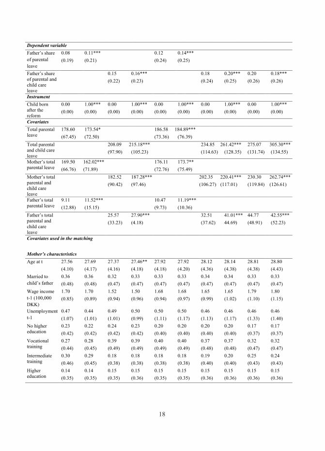
Table 3 shows that this share varies between 8 to 20 percent in my five samples, and that all reforms

except for the one implemented in 2002 increases father’s share of parental leave. Not that the presented

shares are higher than what is found in previous studies on paternity leave in Denmark (e.g. Olsen, 2007),

but this reflect the delimitation of my samples where I only focus on first born children. As I illustrate in

figure 5 below, father’s share of the total leave differs between families with children born before and after

the reform in each sample, with the first four reforms increasing the share, and the last reform reducing the

share (as expected).

Table 3 also shows statistics for the total leave taken by parents during the first year after their child

is born (which I include in the models for reasons specified above). As seen, total leave increases over the

years, from approximately 174 days to 305 days (however with expectedly large differences between the

pure parental leave measure and the combined parental leave and child care leave measure). The table also

includes statistics for mother’s respectively father’s leave. While I do not include these indicators in the

models, I show them to demonstrate exactly how each reform affects the use of parental leave in families. As

shown, the 1989- and the 1997-reforms actually reduce the numbers of days of leave taken by mothers, while

at the same time increasing the days taken by fathers. In contrast, the 1994- and the 1998-reforms increase

both mother’s and father’s leave, and the 2002-reform reduces fathers leave, while increasing mother’s leave

substantially.

Results

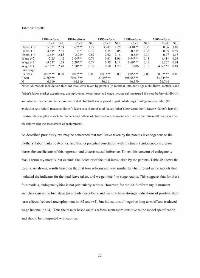
Table 4a shows the results of my analyses when I include the indicator for the total leave taken by the

parents. I run a total of 30 models, reflecting my use of five different reforms, my focus on both short and

longer term labor market outcomes (year t+2 to t+4 from the year of the childbirth) and my use of two

different outcome variables, unemployment and wages. Due to the high number of models, I only present the

coefficient of interest from the second stage model – i.e. the instrumented effect of father’s share of the total

leave on the two outcomes, unemployment and wages. In addition, the lower part of the table shows the

2119

expenses (up to a certain level) through these parental leave benefits (which are registered by employee and

not by employer).

Table 3 shows that this share varies between 8 to 20 percent in my five samples, and that all reforms

except for the one implemented in 2002 increases father’s share of parental leave. Not that the presented

shares are higher than what is found in previous studies on paternity leave in Denmark (e.g. Olsen, 2007),

but this reflect the delimitation of my samples where I only focus on first born children. As I illustrate in

figure 5 below, father’s share of the total leave differs between families with children born before and after

the reform in each sample, with the first four reforms increasing the share, and the last reform reducing the

share (as expected).

Table 3 also shows statistics for the total leave taken by parents during the first year after their child

is born (which I include in the models for reasons specified above). As seen, total leave increases over the

years, from approximately 174 days to 305 days (however with expectedly large differences between the

pure parental leave measure and the combined parental leave and child care leave measure). The table also

includes statistics for mother’s respectively father’s leave. While I do not include these indicators in the

models, I show them to demonstrate exactly how each reform affects the use of parental leave in families. As

shown, the 1989- and the 1997-reforms actually reduce the numbers of days of leave taken by mothers, while

at the same time increasing the days taken by fathers. In contrast, the 1994- and the 1998-reforms increase

both mother’s and father’s leave, and the 2002-reform reduces fathers leave, while increasing mother’s leave

substantially.

Results

Table 4a shows the results of my analyses when I include the indicator for the total leave taken by the

parents. I run a total of 30 models, reflecting my use of five different reforms, my focus on both short and

longer term labor market outcomes (year t+2 to t+4 from the year of the childbirth) and my use of two

different outcome variables, unemployment and wages. Due to the high number of models, I only present the

coefficient of interest from the second stage model – i.e. the instrumented effect of father’s share of the total

leave on the two outcomes, unemployment and wages. In addition, the lower part of the table shows the

20

effect of the instrument (the reforms) on the endogenous regressor (father’s share of the total leave) as well

as the F-test for the excluded instrument. However, both the first and second stage models include all

controls presented in table 2. This may seem redundant given my use of matched samples motivated above,

but I do this to increase precision of standard errors in the models. Note that the coefficients presented in

table 3 might appear rather large, but this reflects the nature of the endogenous regressor: The regressor

varies between 0 and 1 with 1 indicating that father takes all leave. The coefficients then indicate the

difference in mother’s labor market outcomes between household in which father take 0 percent of the leave

and in which fathers take 100 percent of the leave.

Starting from the bottom, we see that the instrument performs well in all models. All reforms significantly

affects fathers share of the total leave, and all F-tests have values above 10. Observe that all reforms

including the one implemented in 2002 positively affects father’s share of the total leave by between 1 and 2

percent. While the first four results comply with expectations, the fifth might seem surprising, given the

expected reform effect and the evidence presented in figure 3. Importantly, though, the coefficient changes

sign (from minus to plus), when I include the indicator of total leave taken by the parents, in the model (as

demonstrated in table 4b). This means that holding constant the total leave, the reform actually increases the

share taken by the father.

Next, focusing on the coefficients from the second stage models, there is a relatively clear pattern, where

results from the specifications relying on the 1994-, 1998- and 2002-reforms suggest that father’s leave

benefits mother’s wages both short, medium and long term. Furthermore, results from the 1989-, 1994- and

the 1997 reform suggests that fathers leave causes an increase in mother’s unemployment in the short run,

while results from the 1994- and the 199 reform suggest that his leave reduces her unemployment in the long

run. Curiously, I get the complete opposite pattern in the specification relying on the 1989-reform, which is

the reform that lead to full wage compensation during leave for those employed in the public sector.

22 21

Table 4a: Results

1989-reform 1994-reform 1997-reform 1998-reform 2002-reform Coef. Std. Coef. Std. Coef. Std. Coef. Std. Coef. Std. Unem. t+2 5.07† 2.59 7.62*** 1.22 3.90† 2.26 -1.01** 0.35 0.06 1.02 Unem. t+3 4.69* 2.35 -0.27 0.79 1.35 2.05 -0.63† 0.33 -0.25 0.97 Unem. t+4 3.62† 2.15 -2.23* 0.87 2.02 2.16 -0.62† 0.34 0.97 1.13 Wage t+2 -2.25 1.42 5.04*** 0.76 0.61 1.06 0.94*** 0.18 1.41* 0.58 Wage t+3 -3.75* 1.68 5.20*** 0.79 0.38 1.14 0.69*** 0.19 1.26* 0.61 Wage t+4 -7.15** 2.40 5.10*** 0.79 0.58 1.20 0.06 0.19 4.36*** 0.84 First stage Ex. Res. 0.02*** 0.00 0.02*** 0.00 0.01*** 0.00 0.05*** 0.00 0.02*** 0.00 F-test 12.86*** 70.01*** 27.89*** 498.95*** 53.34*** N 6,919 44,510 30,011 40,570 36,764 Note: All models include variables for total leave taken by parents (in months), mother’s age a childbirth, mother’s and

father’s labor market experience, unemployment experience and wage income (all measured the year before childbirth),

and whether mother and father are married at childbirth (as opposed to just cohabiting). Endogenous variable (the

exclusion restriction) measures father’s leave as a share of total leave (father’s leave/(mother’s leave + father’s leave)).

I restrict the samples to include mothers and fathers of children born from one year before the reform till one year after

the reform (for the assessment of each reform).

As described previously, we may be concerned that total leave taken by the parents is endogenous to the

mothers’ labor market outcomes, and that its potential correlation with my (main) endogenous regressor

biases the coefficients of this regressor and distorts causal inference. To test this concern of endogeneity

bias, I rerun my models, but exclude the indicator of the total leave taken by the parents. Table 4b shows the

results. As shown, results based on the first four reforms are very similar to what I found in the models that

included the indicator for the total leave taken, and we get nice first stage results. This suggests that for these

four models, endogeneity bias is not particularly serious. However, for the 2002-reform my instrument

switches sign in the first stage (as already described), and we now have stronger indications of positive short

term effects (reduced unemployment in t+2 and t+4), but indications of negative long term effects (reduced

wage income in t+4). Thus the results based on this reform seem more sensitive to the model specification,

and should be interpreted with caution.

23 22

Table 4b: Results

1989-reform 1994-reform 1997-reform 1998-reform 2002-reform Coef. Std. Coef. Std. Coef. Std. Coef. Std. Coef. Std. Unem. t+2 2.23† 1.23 13.11*** 2.90 2.76 1.77 -0.50 0.77 -2.42* 1.03 Unem. t+3 2.09† 1.11 0.58 1.22 0.89 1.58 -0.44 0.72 -1.33 0.95 Unem. t+4 1.63 1.04 -2.38† 1.34 1.42 1.67 -0.79 0.75 -1.80† 1.08 Wage t+2 -0.96 0.73 6.92*** 1.48 0.52 0.81 1.22** 0.41 -0.61 0.53 Wage t+3 -1.71* 0.82 7.10*** 1.53 0.37 0.87 0.25 0.41 0.28 0.57 Wage t+4 -3.48*** 1.04 7.17*** 1.55 0.53 0.92 -1.37** 0.46 -2.50*** 0.71 First stage Ex. Res. 0.03 0.00 0.01 0.00 0.01 0.00 0.02 0.00 -0.02 0.00 F-test 28.47 26.74 19.43 88.42 46.65 N 6919 44510 30011 40570 36764 Note: All models include variables for mother’s age a childbirth, mother’s and father’s labor market experience,

unemployment experience and wage income (all measured the year before childbirth), and whether mother and father

are married at childbirth (as opposed to just cohabiting). Endogenous variable (the exclusion restriction) measures

father’s leave as a share of total leave (father’s leave/(mother’s leave + father’s leave)). I restrict the samples to include

mothers and fathers of children born from one year before the reform till one year after the reform (for the assessment

of each reform).

Eligibility criteria and announcement effects

Importantly, reforms are not only consequential from the day they are installed. Their mere announcement

may change people’s behavior and, in case of the specific reforms exploited in this paper, also eligibility

criteria relating to the child’s birthday are likely to matter. As specified in Table 1, politicians announced the

1994-reform at the end of June 1993 (expanded parental leave), and the 1997-reform (private sector, full

wage compensation) was announced as early as March 1995. In addition, parents of children born from

October 15th 1997 onwards benefitted from the rules specified in the 1998-reform (four weeks earmarked for

fathers), and parents of children born after January 1st 2002 could use the new parental leave scheme

specified in the 2002-reform (less weeks earmarked for fathers, but more leave in total). Hence specifying

the before/after samples according to the reform date may not provide the sharpest distinction of who is and

who is not affected by the reform. This is particularly true with regards to the 1998- and the 2002-reforms,

where parents of children born both before the announcement and the effectuation date are eligible for the

24 23

new rules. But is may also, to a certain extent, be true for the announcement of the 1994-reform, since the

period between the announcement and the effectuation of the reform is sufficiently short to allow parents to

start planning according to the new rules at the time of the announcement (especially since father’s tend to

take the last part of the leave). In contrast, we should not expect the March 1995-announcement of the 1997-

reform to matter much, since the parental leave needs of both the group who had their first child before and

after the announcement are likely to be reduced at the time the reform is installed. Note that I have not been

able to find evidence of the announcement of the 1989-reform.

To test how these alternative dates – reflecting either the eligibility criteria or the announcement of the

reform – matter for the my effects, I rerun my models with re-specified instruments, as described in table 5

below

Table 5: Re-specified instruments

Reform New before group (birth month of child)

New after group (birth month of child)

New reform date reflects

1994 July 1992-June 1993 July 1993-June 1994 Announcement 1997 March 1994-February-1995 March 1995-February-1996 Announcement 1998 November 1996-October 1997 November 1997-October 1998 Eligibility criteria 2002 January 2001-December 2001 January 2002-December 2002 Eligibility criteria

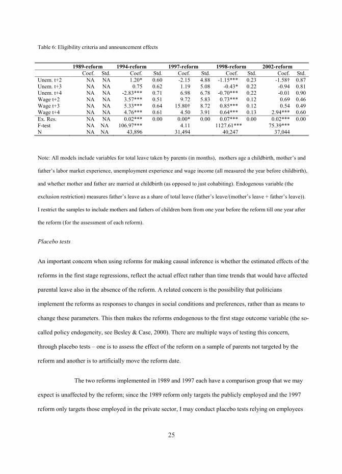
Table 6 shows the results from these new analyses. Looking first at the output from the first stage regression

we see that for the 1994-, the 1998- and the 2002-reform, the instruments remain positive and significant,

and that their power increases compared to what we saw in Table 3, as illustrated by the size of the F-test.

The opposite is true for the instrument specifying the announcement effect of the 1997-reform – the F-test is

considerably lower than the acceptable level of 10 - a finding that is very much in line with expectations, and

which means that we cannot meaningfully interpret the results from the second stage.

The results from the useful second stage models (relying on the 1994-, the 1998- and the 2002-reforms), do

however support previous findings, by showing how an exogenous increase in fathers share of the total leave

taken in the family increases mother’s subsequence wages and to some extent reduces their short, medium

and long run unemployment.

24

Table 6: Eligibility criteria and announcement effects

1989-reform 1994-reform 1997-reform 1998-reform 2002-reform Coef. Std. Coef. Std. Coef. Std. Coef. Std. Coef. Std. Unem. t+2 NA NA 1.20* 0.60 -2.15 4.88 -1.15*** 0.23 -1.58† 0.87 Unem. t+3 NA NA 0.75 0.62 1.19 5.08 -0.43* 0.22 -0.94 0.81 Unem. t+4 NA NA -2.83*** 0.71 6.98 6.78 -0.70*** 0.22 -0.01 0.90 Wage t+2 NA NA 3.57*** 0.51 9.72 5.83 0.73*** 0.12 0.69 0.46 Wage t+3 NA NA 5.33*** 0.64 15.80† 8.72 0.85*** 0.12 0.54 0.49 Wage t+4 NA NA 4.76*** 0.61 4.50 3.91 0.64*** 0.13 2.94*** 0.60 Ex. Res. NA NA 0.02*** 0.00 0.00* 0.00 0.07*** 0.00 0.02*** 0.00 F-test NA NA 106.97*** 4.11 1127.61*** 75.39*** N NA NA 43,896 31,494 40,247 37,044

Note: All models include variables for total leave taken by parents (in months), mothers age a childbirth, mother’s and






Placebo tests

An important concern when using reforms for making causal inference is whether the estimated effects of the

reforms in the first stage regressions, reflect the actual effect rather than time trends that would have affected

parental leave also in the absence of the reform. A related concern is the possibility that politicians

implement the reforms as responses to changes in social conditions and preferences, rather than as means to

change these parameters. This then makes the reforms endogenous to the first stage outcome variable (the so-

called policy endogeneity, see Besley & Case, 2000). There are multiple ways of testing this concern,

through placebo tests – one is to assess the effect of the reform on a sample of parents not targeted by the

reform and another is to artificially move the reform date.

The two reforms implemented in 1989 and 1997 each have a comparison group that we may

expect is unaffected by the reform; since the 1989 reform only targets the publicly employed and the 1997

reform only targets those employed in the private sector, I may conduct placebo tests relying on employees

2523

new rules. But is may also, to a certain extent, be true for the announcement of the 1994-reform, since the

period between the announcement and the effectuation of the reform is sufficiently short to allow parents to

start planning according to the new rules at the time of the announcement (especially since father’s tend to

take the last part of the leave). In contrast, we should not expect the March 1995-announcement of the 1997-

reform to matter much, since the parental leave needs of both the group who had their first child before and

after the announcement are likely to be reduced at the time the reform is installed. Note that I have not been

able to find evidence of the announcement of the 1989-reform.

To test how these alternative dates – reflecting either the eligibility criteria or the announcement of the

reform – matter for the my effects, I rerun my models with re-specified instruments, as described in table 5

below

Table 5: Re-specified instruments

Reform New before group (birth month of child)

New after group (birth month of child)

New reform date reflects

1994 July 1992-June 1993 July 1993-June 1994 Announcement 1997 March 1994-February-1995 March 1995-February-1996 Announcement 1998 November 1996-October 1997 November 1997-October 1998 Eligibility criteria 2002 January 2001-December 2001 January 2002-December 2002 Eligibility criteria

Table 6 shows the results from these new analyses. Looking first at the output from the first stage regression

we see that for the 1994-, the 1998- and the 2002-reform, the instruments remain positive and significant,

and that their power increases compared to what we saw in Table 3, as illustrated by the size of the F-test.

The opposite is true for the instrument specifying the announcement effect of the 1997-reform – the F-test is

considerably lower than the acceptable level of 10 - a finding that is very much in line with expectations, and

which means that we cannot meaningfully interpret the results from the second stage.

The results from the useful second stage models (relying on the 1994-, the 1998- and the 2002-reforms), do

however support previous findings, by showing how an exogenous increase in fathers share of the total leave

taken in the family increases mother’s subsequence wages and to some extent reduces their short, medium

and long run unemployment.

24

Table 6: Eligibility criteria and announcement effects

1989-reform 1994-reform 1997-reform 1998-reform 2002-reform Coef. Std. Coef. Std. Coef. Std. Coef. Std. Coef. Std. Unem. t+2 NA NA 1.20* 0.60 -2.15 4.88 -1.15*** 0.23 -1.58† 0.87 Unem. t+3 NA NA 0.75 0.62 1.19 5.08 -0.43* 0.22 -0.94 0.81 Unem. t+4 NA NA -2.83*** 0.71 6.98 6.78 -0.70*** 0.22 -0.01 0.90 Wage t+2 NA NA 3.57*** 0.51 9.72 5.83 0.73*** 0.12 0.69 0.46 Wage t+3 NA NA 5.33*** 0.64 15.80† 8.72 0.85*** 0.12 0.54 0.49 Wage t+4 NA NA 4.76*** 0.61 4.50 3.91 0.64*** 0.13 2.94*** 0.60 Ex. Res. NA NA 0.02*** 0.00 0.00* 0.00 0.07*** 0.00 0.02*** 0.00 F-test NA NA 106.97*** 4.11 1127.61*** 75.39*** N NA NA 43,896 31,494 40,247 37,044







Placebo tests

An important concern when using reforms for making causal inference is whether the estimated effects of the

reforms in the first stage regressions, reflect the actual effect rather than time trends that would have affected

parental leave also in the absence of the reform. A related concern is the possibility that politicians

implement the reforms as responses to changes in social conditions and preferences, rather than as means to

change these parameters. This then makes the reforms endogenous to the first stage outcome variable (the so-

called policy endogeneity, see Besley & Case, 2000). There are multiple ways of testing this concern,

through placebo tests – one is to assess the effect of the reform on a sample of parents not targeted by the

reform and another is to artificially move the reform date.

The two reforms implemented in 1989 and 1997 each have a comparison group that we may

expect is unaffected by the reform; since the 1989 reform only targets the publicly employed and the 1997

reform only targets those employed in the private sector, I may conduct placebo tests relying on employees

26 25

of the other, unaffected sector. This will also test the concern related to policy endogeneity mentioned above

(however only for these two reforms). For the three other specifications I test whether artificially moving the

reform date affects the results, and for the 1994 and 2002 reforms I test the “reform effect” a year before the

actual reform. However using this strategy with the 1998-reform would collide with the impact of the 1997-

reform, and my robustness check for the 1998 reform therefore consists in moving the reform data a year a

forward in time.

Table 7 shows the results, and as can be seen, for all specifications, we get very poor first

stage results, with insignificant effects of the instrument, and F-test values for the exclusion of the instrument

way below the acceptable threshold value of 10. This then also means that the results from the second stage

are unreliable (notice also their large values which is a classic indication of a weak instrument). These results

provide solid indications that my reform effects do not merely reflect time trends that are also present during

other periods.

Table 7: Results, mother – placebo tests

1989-reform 1994-reform 1997-reform 1998-reform 2002-reform Coef. Std. Coef. Std. Coef. Std. Coef. Std. Coef. Std. Unem. t+2 58.02 42.44 19.45 267.15 -5.13 11.99 1.10 2.54 3.77 3.20 Unem. t+3 28.15 20.57 -198.07 741.06 -0.40 10.55 -0.73 2.41 6.06† 3.43 Unem. t+4 20.52 17.02 -226.26 1267.77 1.08 9.69 0.30 2.43 8.37* 4.25 Wage t+2 -32.42 24.08 169.34 1013.51 9.21 14.89 -0.84 1.31 -3.71† 1.98 Wage t+3 -29.84 22.29 -41.34 249.35 6.10 11.39 -9.74*** 3.53 2.12 1.74 Wage t+4 -43.27 31.88 -187.70 1124.40 8.81 14.55 -9.59*** 3.53 2.88 1.92 Ex. Res. 0.00 0.00 0.00 0.00 0.01 0.01 0.01** 0.00 0.01** 0.00 F-test 1.97 0.01 0.50 9.41 7.17 N 14912 43632 1505 40211 38465 Content Couples with no

public sector affiliation

A year before announcement

Couples with no public sector affiliation

A year after announcement

A year before announcement







27 26

Conclusion

This paper departs from the growing literature on how father’s paternity leave affects mother’s subsequent

labor market outcomes, and offers a new approach to understanding when father’s take up of paternity leave

may matter. By claiming that father’s leave only matters if it changes the relative distribution of labor market

respectively domestic capital in the household, I refrain from looking at the effect the actual days, weeks or

months that fathers spend on paternity leave, but focus on how many days he spends relative to how many

days the mother spends. For this purpose, I exploit a series of reforms of the Danish parental leave system

that change the total months of leave available for Danish parents, and introduces or removes earmarked

leave for fathers. These reforms facilitate exogenous variation in both fathers’ and mothers’ take up of leave

and enables causal inference.

Overall, my results indicate a positive effect of fathers’ leave on mothers’ labor market

outcomes, even if one reform – the reform granting employees in the public sector full wage compensation in

1989 – points in the complete opposite direction. Hence the majority of my results reflect the theoretical

predictions presented earlier that when the father improves his domestic capital relative to the mother, and at

the same time, reduces his own labor market capital (relative to her’s), it counteracts (part of) the

motherhood penalty.

Importantly though, some of the reforms used in this paper concern specific groups at the labor market – e.g.

the 1989-reform targets employees in the public sector, while the 1997-reform targets employees in the

private sector – and this may explain some of the inconsistency in the results. Not only will different sectors

be dominated by different types of families with different values concerning family life and gender role

ideologies, they also have different starting points concerning pre-reform take up rates. Hence the margin

affected by each reform will vary, which means that we cannot expect all LATE estimates to point in the

same direction. Still, it is quite reassuring that we get a relatively consistent picture of the effects across

specifications.

28 27

Literature:

Aisenbrey, Silke, Evertsson, Marie & Grunow, Daniela (2009): Is There a Career Penalty for Mothers’ Time

Out? A Comparison of Germany, Sweden and the United States. Social Forces, 88(2): 573-605

Becker, Gary S. (1981): A Treatise on the Family. Harvard University Press

Besley, Timothy & Case, Anne (2000): Unnatural experiments? Estimating the incidence of endogenous

policies. The Economic Journal, 110: 672-694

Bonke, Jens, Datta Gupta, Nabanita & Smith, Nina (2004): Timing and Flexibility of Housework and Men

and Women’s Wages. In D.S. Hamermesh and G. A. Pfann (eds.). Contributions to Economic Analysis, vol.

204. Elsevier Press.

Budig, Michelle J. & Hodges, Melissa J. (2010): Differences in Disadvantage: Variation in the Motherhood

Penalty across White Women’s Earnings Distribution. American Sociological Review, 75(5): 705-728

Cools, Sara, Fiva, Jon H. & Kirkebøen, Lars Johannessen (2011): Causal effects of paternity leave on

children and parents. Statistics Norway, Research Department Discussion Papers, no. 657

Datta Gupta, Nabanita, Smith, Nina & Verner, Mette (2008): The impact of Nordic countries’ family friendly

policies on employment, wages, and children. Review of Economics of the Household, 6: 65-89

Datta Gupta, Nabanita Datta & Smith, Nina (2002): Children and Career Interruptions: the Family Gap in

Denmark. Economica, 69(276): 609-629

Ekberg, John, Eriksson, Rickard & Friebel, Guido (2005): Parental Leave – A Policy Evaluation of the

Swedish “Daddy-Month” Reform. IZA Discussion Paper, 1617

Evertsson, Marie & Duvander, Ann-Zofie (2010): Parental Leave – Possibility or Trap? Does Family Leave

Length Effect Swedish Women’s Labour Market Opportunities? European Sociological Review, 27(4): 435-

450

29 28

Gangl, Markus & Ziefle, Andrea (2009): Motherhood, Labor Force Behavior, and Women’s Careers: An

Empirical Assessment of the Wage Penalty for Motherhood in Britain, Germany and the United States.

Demography, 46(2): 341-369

Hansen, Anette Eklund (2003): Barselsorlovens historie i 100 år. Found at www.aba.dk

Jacobsen, Sara Jul, Klynge, Alice Heegaard & Holt, Helle (2013): Øremærkning af barsel til fædre. Et

litteraturstudie. København: SFI, 13:22

Johansson, Elly-Ann (2010): The effect of own and spousal parental leave on earnings. IFAU Working

Paper, 2010:4

Kahn, Joan R., García-Mangland, Javier & Bianchi, Suzanne M. (2014): The Motherhood penalty at Midlife:

Long-Term Effects of Children on Women’s Careers. Journal of Marriage and Family, 76: 56-72

Karu, Marre (2012): Parental Leave in Estonia: Does Familization of Fathers Lead to Defamilization of

Mothers? NORA – Nordic Journal of Feminist and Gender Research, 20(2): 94-108.

Kotsadam, Andreas & Finseraas, Henning (2011): The State Intervenes in the Battle of the Sexes. Causal

Effects of Paternity Leave. Social Science Research, 40(6): 1611-1622.

Lalive, Rafael, Schlosser, Analía, Steinhauer, Andreas & Zweimüller, Josef (2011): Parental Leave and

Mothers’ Careers: the relative Importance of Job Protection and Cash Benefits. IZA Discussion Paper, 5792

Lundberg, Shelly & Rose, Elaina (2000): Parenthood and the earnings of married men and women. Labour

Economics, 7: 689-710

Nielsen, Helena Skyt, Simonsen, Marianne & Verner, Mette (2004): Does the Gap in Family-friendly

Policies Derive the Family Gap. Scandinavian Journal of Economics, 106(4): 721-744

Olsen, Bente Marianne (2000): Nye fædre på orlov. Sociologisk Institut, Københavns Universitet

Olsen, Bente Marianne (2007): Evaluering af den fleksible barselsorlov. SFI 07:29

30 29

Patnaik, Ankita (2015): Reserving time for daddy: The short and long-run consequences of fathers’ quotas.

Available at SSRN: http://ssrn.com/abstract=2475970

Pertold-Gebicka, Barbara, Pertold, Filip & Datta Gupta, Nabanita (2016): Employment Adjustments around

Childbirth. IZA Discussion Paper, no. 9685

Pylkkänen, Elina & Smith, Nina (2003): Career Interruptions due to Parental leave: A Comparative Study of

Denmark and Sweden. OECD SOCIAL, EMPLOYMENT AND MIGRATION WORKING PAPERS, 2003(1)

Rasmussen, Astrid Würtz (2010): Increasing the length of parents’ birth related leave: The effect on

children’s longterm educational outcomes. Labour Economics, 17(1): 91-100

Rege, Mari & Soli, Ingeborg F., (2013): The Impact of Paternity Leave on Fathers’ Future Earnings.

Demography, 50: 2255-2277

Schober, Pia S. (2014): Daddy leave: does it change the gender division of domestic work? DIW Roundup,

46

Staff, Jeremy & Mortimer, Jeylan T. (2012): Explaining the Motherhood Wage Penalty During the Early

Occupational Career. Demography, 49(1): 1-21

Ugreninov, Elisabeth (2013): Can Family Policy reduce Mothers’ Sick Leave Absence? A Causal Analysis

of the Norwegian Paternity Leave Reform. Journal of Family and Economic Issues, 34(4): 435-446

Paternity leave and the motherhood Penalty: new causal ... · This paper contributes to the...

Documents

Transcript of Paternity leave and the motherhood Penalty: new causal ... · This paper contributes to the...