International Journal of Computers and Applications, Vol. 31, No. 2, 2009

PASSIVE ATMOSPHERIC DIFFUSION

WITH GAUSSIAN FRAGMENTATION

S.S. Beauchemin,∗ H.O. Hamshari,∗ and M.A. Bauer∗

Abstract

Events such as atmospheric gas dispersion by industrial accidents

or processes are generally predicted with Gaussian plumes, coupled

with local models of gas emission. In this contribution we inves-

tigate the association of integral models of instantaneous emission

with Gaussian dispersion processes for predicting the progression of

potentially hazardous low-altitude emissions over sensitive or popu-

lated areas. We develop a novel, more accurate approach suitable for

dynamic, high spatial resolution atmospheric conditions by means

of gas plume fragmentation and parallel estimation of extent and

concentration.

Key Words

Parallel simulation, integral model, atmospheric plume, Gaussian

cloud, Hexagonal sphere packing

1. Introduction

Because of its simplicity, the Gaussian dispersion modelis often used for predicting the progression of atmosphericgas plumes [1–3]. This model relies on a number ofhypotheses to determine the path and spread of plumes,the most fundamental stating that the dispersion must bepassive, which is equivalent to considering the gas densityas roughly the same as that of the surrounding atmosphere.

Before reaching the stage of passive dispersion, initialconditions of gas emissions are often addressed differently,as various gases may have densities differing from ambientair (depending on molecular weight, temperature, altitudeof emission, and so on). Failing to consider such parametersin the early stages could result in considerable predictionerrors, either in concentration levels or geographical spread.

The use of Gaussian dispersion models requires thatterrain be free of significant obstacles such as skyscrapersor mountain ranges, or that the altitude of the emissionsource be sufficiently high to ignore obstacles. Otherhypotheses include the absence of atmospheric turbulenceand gas densities which minimize the effect of gravity onthe plume. Under such conditions, the dispersion results

∗ Department of Computer Science, The University of WesternOntario, 1151 Richmond Street, London ON N6A 5B7; e-mail:beau@csd.uwo.ca, hohamsha@uwo.ca, bauer@csd.uwo.ca

Recommended by Prof. Shaharuddin Salleh(paper no. 202-2338)

are usually considered correct from approximately 100mfrom the emitting source and beyond [4].

Hence, in our low-altitude emission framework, the soleuse of a Gaussian dispersion model is clearly inadequate.A local emission model for the source is required, andwe adopt the integral model as an instantaneous emissionsource, which aptly provides the initial conditions for theGaussian dispersion simulation. An additional hypothesispertaining to the integral model requires that gas emissionbe relatively significant, generally in the order of a fewm3/s. A gas cloud following an integral model evolvesat very small spatio-temporal scales while compared withthe much larger dispersion extents inherent to a Gaussianmodel. However, the integral model is required, if onlyto provide the dispersion process with adequately realisticinitial parameters.

The integral model employs a stack of cylinders, de-scribing volumes (or puffs) containing gas particles. Thesepuffs are updated through an iterative process until theyreach the density of the surrounding air. Ultimately, puffswith such densities are injected in the stack of the Gaus-sian model, for large-scale dispersion computations tobegin.

To combine the integral and Gaussian models whilepreserving a relative flexibility, we choose an approach inwhich both models share common environmental param-eters, operating over a discretized grid map describingdynamic atmospheric and terrain conditions. At each it-eration, the combined model updates the environmentalconditions and the characteristics of emission sources, andinjects gas puffs in the integral or Gaussian model. Resultsare expressed as concentration and dispersion grids overthe region of interest.

This contribution presents a combined integral–Gaussian model which includes Gaussian puff fragmenta-tion. The process of fragmentation consists of breaking uplarge Gaussian puffs into sets of smaller ones, to increasethe accuracy of plume simulations: Gaussians puffs cover-ing large geographical extents (1 km or more) are generallysubjected to spatially variable winds within their extent,while puffs with smaller extents are less likely to sufferfrom this phenomenon. Consequently, a plume composedof many small puffs will evolve along the prevailing windsmore accurately than plumes composed of puffs withsignificant extents.

97

We proceed by presenting a survey of the related lit-erature, the integral and Gaussian models, the fragmenta-tion process, and experiments from our atmospheric plumesimulator.

2. Related Literature

Several models of passive air dispersion exist, and they maybe organized according to their level of mathematical com-plexity [2]. Among the typical classes of dispersion mod-els, we find: gross screening models, intermediate models,and advanced models, as per their degree of mathematicalsophistication.

Gross screening models are those that require the sim-plest tools and are generally used in the absence of moreelaborate models to make worst-case predictions [2]. Thesophistication of the input data is minimal and allows emer-gency planners to make crude estimations in a minimum oftime. For instance, this class of models includes Hanna etal.’s work on the estimation of worst mean concentrationdownwind from a point source [5].

Intermediate models are able to take into accountatmospheric stability classes and wind speed as inputs.This class is represented by models such as the diffusionequation, which describes smoke behaviour in turbulentair flows [6]. Analytical solutions to this diffusion equationinclude the Gaussian plume model in its simplest form forcontinuous point sources [3].

The Gaussian plume model is central to the modellingof atmospheric diffusion, and one of the remaining diffi-culties associated with its use is the determination of ade-quate diffusion coefficients (Gaussian standard deviations),which depend on local conditions at and around the site ofrelease. This problem has been investigated since the firstuses of this model. For instance, Barad was one of the firstto determine adequate values for the diffusion parametersin prairie-like terrain conditions [7, 8]. Based on this work,Pasquill and Gifford proposed coefficients for releases atlow altitude over relatively obstacle-free terrains [9, 10].They examined the turbulence created by the heating ofthe atmosphere from the ground and defined atmosphericstability classes, for both daytime and night-time releases.While Pasquill and Gifford’s results could be used over rel-atively flat terrains, McElory and Pooler contributed coeffi-cient curves and tables for diffusion in urban environmentswhich were much needed at the time [11].

Elaborate diffusion coefficients may also be derivedwhen atmospheric conditions are known with precision.For instance, Draxler and others have related the valuesof the coefficients to velocity variation directly [12–14], toaccount for the increased turbulence and dispersion thesefluctuations create.

Advanced models of passive diffusion include complexatmospheric phenomena such as plume ground reflection,elevated inversion, advection velocity, and plume rise withdown-wash [2]. In the case of ground reflection, an elevatedrelease will diffuse vertically until the bottom of the plumereaches the ground, where gas particles are reflected, orabsorbed. In addition, as the plume elevates, it mayreach an atmospheric temperature inversion, effectively

dampening its ascension. When both phenomena arecombined, the plume mostly remains in a layer comprisedbetween the ground and the inversion. In practice, theconcentration in the layer tends to reach uniformity, andcan be estimated accordingly [3]. More recently, techniqueshave been designed to account for situations in which aplume is only partially reflected by an inversion [15].

From the ground to low altitudes, wind speed varieslogarithmically and in turn influences plume velocity [16].This effect is generally approximated with a power law, inwhich the value of the exponent is strongly influenced bythe atmospheric stability class and the ground roughness,as noted by Irwin [17]. Atmospheric stability also hasan effect on the mean wind profile and is taken intoconsideration by advanced passive diffusion models, usingthe Monin-Obukhov scale of meteorological parameters [5].

Initial release momentum and plume buoyancy gener-ally cause a plume to rise rapidly, before prevalent windsmake it bend in the downwind direction. Correctionshave been suggested to include release momentum andbuoyancy in advanced models by considering the effectiveheight of the release, which varies with the intensity of thedown-wash [18]. Simplifying assumptions, introduced byDavidson, must be posed to obtain closed-form equationsfor buoyant plumes [19].

While these techniques improve the performance ofpassive diffusion models, a problem subsists when thespatial extents of Gaussian puffs become so large as toencompass regions in which atmospheric conditions mayvary substantially. Our research addresses this problemby establishing a Gaussian puff-breaking technique whichmay be employed to keep the maximum size of puffsas a constant, resulting in plumes composed of elementssmall enough to remain under consistent meteorologicalconditions.

3. The Integral Model

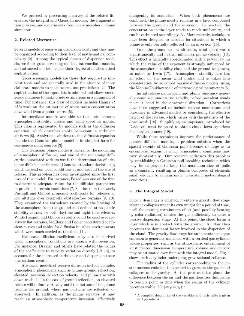
Once a dense gas is emitted, it enters a gravity flow stagewhere it collapses under its own weight for a period of time,until the ensuing entrainment of air (and possibly heatingby solar radiation) dilutes the gas sufficiently to enter apassive dispersion stage. At this point, the cloud forms alayer which is in contact with the ground. Air flow thenbecomes the dominant factor involved in the dispersion ofthe cloud. The gravity flow stage for an instantaneous gasemission is generally modelled with a vertical gas cylinderwhose properties, such as the atmospheric entrainment ofair it creates, dimension, temperature, volume, and densitymay be estimated over time with the integral model. Fig. 1shows such a cylinder undergoing gravitational collapse.

The radius of the cylinder corresponding to the in-stantaneous emission is expected to grow, as the gas cloudcollapses under gravity. As this process takes place, thedifference between the air and the gas densities diminishesto reach a point in time when the radius of the cylinderbecomes stable [20] (at ρ= ρa)

1:

1 A complete description of the variables and their units is givenin Appendix A.

98

Figure 1. Collapse of gas cylinder under various environ-mental and gravitational effects.

R′ = K

√gH

ρ− ρaρa

(1)

The total mass of air entrained by the gas cloud, whichsignificantly contributes to its dilution, evolves in time ata rate given by:

M ′a = πρa

(R′2α1HR+R2α2

Ut

R1

)(2)

The entrainment of air is a function of the areas of the edgeand top of the cylinder, as well as the speed of turbulentair.

The temperature of the cloud is influenced by variousfactors, the most significant being the temperature of theground (Q1) with which the gas is in contact, and thetemperature of the surrounding air (Q2):

T ′ =Q1 +Q′

2

MaCa +MgCg(3)

It is assumed that turbulent convection is the means bywhich heat is supplied to the gas from the ground:

Q1 = α3(T − Ts)43 (4)

The heat transfer between the air and the cloud is expressedas:

Q′2 = M ′

aCa(Ta − T ) (5)

From previous equations, we can derive the volume, height,mean concentration, and density of the cloud:

V =Ma +Mg

ρ(6)

H = πV

R2(7)

C =Mg

V(8)

ρ = T (Ma +Mg)T−1a

(Ma

ρa+

Mg

ρg

)−1

(9)

The integral model is adequately suited for dense gasdispersions until the difference in gas and air densitiesbecomes negligible. At this point, the model provides theinitial parameters to a passive dispersion calculation, suchas that carried out by a Gaussian model.

4. The Gaussian Model

The simplest form of atmospheric dispersion is passive.Nonetheless, determining the standard deviations for theGaussian model in realistic cases remains a complex andexperimental problem. According to Pasquill’s experi-ments [9, 21], the initial standard deviations σy and σz

(the crosswind and the vertical dispersion coefficients2,respectively) for the Gaussian model can be computed as:

σy or σz = axb + c (10)

where x, the distance from the source, is expressed inkilometres. Values for parameters a, b, and c are obtainedfrom Tables 1 and 2, according to six atmospheric stabilityclasses, from A (very unstable) to F (very stable). Thevalues of these parameters differ whether σy or σz iscomputed. Atmospheric stability depends on factors suchas wind speed, incident solar radiation, cloud cover, andpossibly ground roughness at low altitudes. Tables 3 and4 give the atmospheric stability class as a function of windand solar radiation for daytime and as a function of windand cloud cover for night-time. Once σx, σy, and σz arecomputed and the simulation is ongoing, concentrationsmay be estimated at a given time step with the followingGaussian:

C(x) =M

(2π)32 detS

exp

{−1

2[S−1(x− xc)]

TS−1(x− xc)

}(11)

where

S =

⎛⎜⎜⎜⎝

σx 0 0

0 σy 0

0 0 σz

⎞⎟⎟⎟⎠

is the matrix of dispersion coefficients. Concentration isobtained at x=(x, y, z)T while the centre of the Gaus-sian is located at xc =(xc, yc, zc)

T . As the wind pushesthe Gaussian cloud, its centre is updated with the pre-vailing wind velocity vector u. In addition, the distancex from the source to the centre of the Gaussian cloud isrecomputed as3:

2 Pasquill assumed σx =σy , which is a reasonable hypothesis forcrosswind dispersion.

3 The initial dispersion coefficients for the Gaussian are providedby the integral model after the gas cylinder has collapsed.Hence, the position of the source is said to be virtual, as itdoes not reflect the position of the gas cylinder.

99

Table 1Standard Deviations According to Pasquill’s AtmosphericStability Classes, for Passive Dispersions under 1 km [21]

x≤ 1 km

Class σ a b c

A σy 0.215 0.858 0.00σz 0.467 1.890 0.01

B σy 0.155 0.889 0.00σz 0.103 1.110 0.00

C σy 0.105 0.903 0.00σz 0.066 0.915 0.00

D σy 0.068 0.908 0.00σz 0.032 0.822 0.00

E σy 0.050 0.914 0.00σz 0.023 0.745 0.00

F σy 0.034 0.908 0.00σz 0.014 0.727 0.00

Table 2Standard Deviations According to Pasquill’s AtmosphericStability Classes, for Passive Dispersions over 1 km [21].Standard Deviations for Classes A through D are as

per Table 1

x> 1 km

Class σ a b c

E σy 0.050 0.914 0.00

σz 0.148 0.015 −1.126

F σy 0.034 0.908 0.000

σz 0.031 0.306 −0.017

Table 3Daytime Atmospheric Stability Class as a Function of

Wind and Solar Radiation

Wind Solar Radiation (Wm2)

(m/s) ≥925 925–675 675–175 ≤175

<2 A A B D

2–3 A B C D

3–5 B B C D

5–6 C C D D

>6 C D D D

x =

(σx − c

a

) 1b

(12)

This description of the Gaussian model accounts forone instantaneous emission of gas only. A source emit-

Table 4Nighttime Atmospheric Stability Class as a Function of

Wind and Cloud Cover

Wind Cloud Cover (%)

(m/s) ≥50 <50

<2 F F

2–3 E F

3–5 D E

>5 D D

Table 5Values for z′0 Depend on Terrain Roughness

Flat Terrain z′0 = z0

Agricultural Land z′0 ≈ 0.10m

Garden Area z′0 ≈ 0.30m

Residential Area z′0 ≈ 1.00m

Urban Area z′0 ≈ 3.00m

ting in a continuous fashion must be modelled differently.The instantaneous integral and Gaussian models can beextended to include series of instantaneous emissions overtime, each emission at time ti possessing its own mass of gasMi. Hence, to simulate a continuous emission, the integralmodel is fit with a gas cylinder stack while the Gaussianmodel receives a puff stack. Each new emission is placed inthe gas cylinder stack, where the simulation begins. Whena cylinder has reached relative stability, its parameters arefed into the puff stack of the Gaussian model, where it isleft to develop according to prevailing environmental con-ditions. The resulting set of instantaneous emissions formsa plume governed by passive dispersion.

These models are obvious simplifications of environ-mental reality which entails more complex phenomena suchas ground reflection and roughness, and particle fallout [4].

4.1 Ground Roughness

Variations in terrain quality, from plains to dense urban ar-eas, affect the dispersion of gaseous puffs through increasedturbulence. A correction, applied to the dispersion coeffi-cients and introduced by Pasquill and Smith [21], amountsto computing the coefficient σz as:

σz = (axb + c)

(z′0z0

)0.53x−0.22

(13)

where z′0 is a measure of ground roughness expressed in m,and z0 is a constant set to 0.03m. Table 5 indicates appro-priate values for z′0 with respect to terrain characteristics.

100

4.2 Ground Reflection

The ground may not entirely reflect gas particle fallouts,depending on gas and terrain properties. In light ofthis, a reflection correction is introduced, accounting forthe resulting reduction in concentration as gas particlesprecipitate to the ground. This correction transforms theexponential in z from (11) into:

exp

{− (z − zc)

2

2σ2z

+ ρ(z + zc)

2

2σ2z

}(14)

where zc is the emission height in metres and ρ is groundreflection coefficient.

The rate of change in gaseous mass due to fallout canbe obtained with:

M ′ =(r − 1)M√

2π

(σz

z2 + 2σ2z

+1√2tan−1 z√

2σz

)(15)

evaluated between zc and zc +σz|t+δt

σz|t . Coefficient r repre-

sents ground reflection, which assumes values between 0.0for no reflection, up to 1.0 for complete reflection.

4.3 Model Interface

There are several ways of combining the integral and theGaussian model [21], and we adopted a method which posesthe least number of hypotheses on the emission process.Once a gas cylinder has collapsed under gravity and itsdensity has become similar to that of the surroundingair, the simulation must then turn to a passive mode, inthe form of a 3D Gaussian puff. The interface residesin determining the initial parameters for the Gaussianfrom the integral model. At this critical stage, the gasmass must be conserved, and the parameters that requireadjustments are the dispersion coefficients that are foundin the covariance matrix S of (11). Experiments have leadto the following relationships between the cylinder heightand radius and the dispersion coefficients [4]:

R = 2.14σy (16)

H = 2.14σz (17)

The initial position of the puff is given by the coordinatesof the centre of the collapsed cylinder. In the passivemode of diffusion, the parameters requiring updating arethe position of the puff, its mass (due to fallout), and itsdispersion coefficients, from environmental variables suchas ground roughness, reflection, direction and speed ofprevailing winds, and so on.

5. Puff Fragmentation

The Gaussian model, when used to predict continuousemissions, possesses a relative adaptability as each puffevolves with respect to its local environmental conditions,provided that these are available on such a local scale.Over time, the scale of Gaussian puffs increases to a point

Figure 2. The positional symmetries of the top layer puffsstarting at the bottom centre of the initial cloud.

Figure 3. The positional symmetries of the middle layerpuffs starting at the bottom centre of the initial cloud.

Figure 4. The positional symmetries of the bottom layerpuffs starting at the bottom centre of the initial cloud.

where atmospheric conditions within their extent may varysignificantly. To account for such variation, an effectiveapproach consists of fragmenting large Gaussian puffs intosmaller ones, while preserving the properties of the plume,such as spread and concentration. The original Gaussianpuff prior to the fragmentation is represented by an ellip-tical sphere. We use a hexagonal sphere packing schemeto create a group of elliptical spheres, each a Gaussianpuff, with a distribution as close to the original Gaussianas possible. This fragmentation ensures a minimal numberof elliptical spheres with relative positional symmetries.Figs. 2–4 show such a fragmentation, along with positionalsymmetries of the sphere centres for an initial Gaussianpuff centreed at coordinates xc =(0, 0, 0)T .

101

Figure 5. The computation of sphere centres. (a) Theradius of the inscribed equilateral triangle formed by thecentres of spheres r0, r1, and r2, yields the x, y coordinatesof sphere r7 from the top layer and (b) the height of thetetrahedron formed by the centres of spheres r0, r1, r2,and r7 yields the z coordinate of sphere r7.

5.1 Computing Gaussian Sphere Centres

Let C(x) be a 3D Gaussian with covariance matrix S, asin (11). After fragmentation into a hexagonal packing, the13 resulting Gaussians have covariance matrices Sf =

23S

with the centre coordinates of the centre Gaussian set tor0 =(0, 0, 0)T . The x, y plane contains the centres of thesix Gaussians surrounding r0, labeled clockwise from r1 tor6 starting with the top one on the y-axis, as per Fig. 5(a).

The centre coordinates of Gaussian r1 are immediately

obtained as: r1 =S(0, 2

3 , 0)T

. The rightmost point of thedotted equilateral triangle with side 2r

(or 2

3

)shown in

Fig. 5(a) yields the x, y coordinates of Gaussian r2. They coordinate is equal to r

(or 1

3

), and the x coordinate

is obtained as x2 + r2 =(2r)2. Hence, x=√33 and the

centre of r2 is S(√

33 , 1

3 , 0)T

. The centre coordinates

of r3 and r4 are obtained by folding around the x-axis

as r3 =S(√

33 , −1

3 , 0)T

and r4 =S(0, −2

3 , 0). The centre

coordinates of r5 and r6 are obtained by folding around

the y-axis as r5 =S(

−√3

3 , −13 , 0

)Tand r6 =S

(−√

33 , 1

3 , 0).

The top layer consists of three Gaussian spheres thatare packed hexagonally from the central layer, as inFig. 5(b). The first sphere r7 is in contact with centrallayer spheres r0, r1, and r2 and its x centre coordinate isgiven by the radius of the inscribed circle inside the dotted

triangle:√39 . As the sides of the triangle are 2r in length,

the y coordinate is given by r or 13 . The z coordinate can

be obtained as the height of the tetrahedron of side 2rformed by the centres of Gaussian spheres r0, r1, r2, and

r7 as2√6

9 (depicted in Fig. 5(b)). Hence, the coordinates of

r7 are S(√

39 , 1

3 ,2√6

9

)T. Progressing clockwise, the second

sphere r8 of the top layer is in contact with spheres r0, r3,and r4 from the central layer, and its centre coordinates

are obtained by folding the x-axis: r8 =S(√

39 , −1

3 , 2√6

9

)T.

Sphere r9 is in contact with spheres r0, r5, and r6 of thecentral layer. Due to its placement, the y coordinate of thecentre of this sphere is simply 0. In addition, because thethree Gaussian spheres from the top layer are equidistantfrom the point (x, y)= (0, 0), its x coordinate is obtained asthe negative of the length of the segment from (x, y)= (0, 0)to the centre of sphere r7, projected onto the x, y plane:

−2√3

9 . Hence, r9 =S(

−2√3

9 , 0, 2√6

9

)T. Fig. 6(a) shows the

final placement of the Gaussian spheres from the top layer.As there are only two ways of placing the top or the

bottom layer with respect to the central one, we chose toplace the bottom layer in a different configuration fromthe top layer, to achieve symmetry of concentration in theGaussian sphere pack. To this end, sphere r10 is placedsuch as to create contact with spheres r0, r1, and r6 fromthe central layer. Its centre coordinates are immediately

obtained by symmetry as r10 =S(

−√3

9 , 13 ,

−2√6

9

)T. The

centres for r11 and r12 are obtained symmetrically as

r11 =S(

2√3

9 , 0, −2√6

9

)T, and r12 =S

(−√

39 , −1

3 , −2√6

9

)T.

Fig. 6(b) shows the final placement of the spheres fromthe bottom layer, while Figs. 2–4 show the positionalsymmetries of the Gaussian sphere pack.

5.2 Error Minimization

This Gaussian puff fragmentation scheme must maintainessential properties such as the conservation of both thetotal gaseous mass and the geographical distribution ofconcentrations. To this end, our initial, empirically deter-mined approximation consists of a central puff containing21.81% of the initial gaseous mass with the remaining 12puffs containing 6.52% each. The dispersion coefficientsσx, σy, and σz from each of the 13 puffs are set to 2

3 of theinitial cloud coefficients, while the sphere centres are setto kfri:

C =M

(2π)32 detS

exp

{−1

2[S−1(x− xc)]

TS−1(x− xc)

}

≈12∑i=0

Mi

(2π)32 detSf

exp

{−1

2[S−1

f (x− xc − kfri)]T

S−1f (x− xc − kfri)

}(18)

102

Figure 6. (a) The top layer sphere arrangement and (b)the bottom layer sphere arrangement.

where Sf = kσS, kσ =23 , kf =π

23 ,

Mi =

⎧⎨⎩0.218107 if i = 0

0.065158 otherwise

and

r0 = S(0, 0, 0)T

r1 = S

(0,

2

3, 0

)T

r2 = S

(√3

3,1

3, 0

)T

r3 = S

(√3

3,−1

3, 0

)T

r4 = S

(0,

−2

3, 0

)T

r5 = S

(−√

3

3,−1

3, 0

)T

r6 = S

(−√

3

3,1

3, 0

)T

r7 = S

(√3

9,1

3,2√6

9

)T

r8 = S

(√3

9,−1

3,2√6

9

)T

r9 = S

(−2

√3

9, 0,

2√6

9

)T

r10 = S

(−√

3

9,1

3,−2

√6

9

)T

r11 = S

(2√3

9, 0,

−2√6

9

)T

r12 = S

(−√

3

9,−1

3,−2

√6

9

)T

While approximation (18) preserves the total gas mass,the distribution of concentrations still slightly varies fromthe initial Gaussian puff, as shown by the error functionin Fig. 7. Hence, we defined a functional to be minimizedwith respect to kσ and kf , which are the parameters thatinfluence the distribution of concentration the most:

F (kσ, kf ) =1

(2π)32

∫ ∞

−∞

[M

detSexp

{−1

2[S−1(x− xc)]

T

S−1(x− xc)

}

−12∑i=0

Mi

detSfexp

{−1

2[S−1

f (x− xc − kfri)]T

S−1f (x− xc − kfri)

}]2dx (19)

We used Polak-Ribiere’s conjugate-gradient descentmethod to minimize (19) with respect to kσ and ff . Theprocedure lead to the following values: kσ =0.754529 andkf = 1.8303234. The resulting error function displayed inFig. 8 evaluated to 4.01E−4 and shows the improvementover our initial approximation, illustrated in Fig. 8.

4 The choice of keeping the mass distribution constant overthe minimization process is motivated by the fact that theinclusion of these terms invariably leads to a central fragmentedGaussian sharing its parameters with the initial one (massand dispersion coefficients), and a zero mass for the remainingfragmented Gaussians.

103

Figure 7. The Gaussian fragmentation process using our initial parameters kσ and kf . The 13 Gaussians generated afterfragmentation of the initial Gaussian: (a) the centre layer, (b) the top layer, (c) the bottom layer, (d) the Gaussian prior tofragmentation, followed by (e) the sum of the 13 Gaussians, and (f) the error function.

Figure 8. The results obtained with the minimization of the error functional: (a) the Gaussian prior to fragmentation,followed by (b) the sum of the 13 Gaussians, and (c) the error functional.

6. Parallelization

From a computational standpoint, the combined integral–Gaussian model with puff fragmentation is demanding,particularly when the number of Gaussian puffs becomes

large. Fortunately, the model lends itself rather naturallyto parallelization.

A number of observations concerning the characteris-tics of the combined model can be made: during a simula-tion, the integral model is in use for what amounts to be

104

Figure 9. (a) Classical plume progression from a continuous emission source and (b) plume progression with Gaussian pufffragmentation. Different trajectories under identical wind vector fields are experienced.

a small duration per emitted gas cylinder, owing to rapidcollapse and dilution. In comparison, the Gaussian modelis computationally costlier, due to the number of Gaussianpuffs fed to its stack by the integral model, the duration ofeach puff (hours, perhaps days), and particularly the pufffragmentation mechanism, which exponentially increasesthe number of puffs entering the simulation. In addition,one of the most demanding processes is the calculation ofestimated concentrations over grid maps.

Consider a continuous gaseous emission lasting a totaltime T =N1t, with a Gaussian puff emitted at every t. Thetotal number of puffs, without fragmentation is thus N1.If we assume that each puff is fragmented n times, then N ,the number of Gaussian puffs in the simulation is:

N = N1

n∑i=0

P i (20)

where P =12. For instance, if 1,000 initial puffs are re-leased, after four simultaneous fragmentations, the numberof puffs in the simulation reaches 22,621,000. In addition,numerous concentration calculations must be carried outfor each puff, and the amount of these increases as theextent of the puffs becomes larger. A monoprocessor ar-chitecture is clearly inadequate for long simulations suchas radiological emissions and volcanic phenomena, whichmay last for days.

An adequate parallel architecture for the paralleliza-tion of the combined integral–Gaussian model is a shared-memory, multiprocessor architecture allowing computingunits to share one instance of the grid map of the regionof interest, while ensuring an adequate distribution of thecomputation of dispersion and concentration. For instance,the puffs could be evenly distributed among available pro-cessors in a natural fashion each time they are introducedin the simulation. In the context of the preceding example,a multiprocessor architecture with 210 available computingunits would, at the peak of the simulation, reduce the com-

puting load from 22 million puffs to 22,091 per processor,which is an acceptable computational burden.

7. Experiments

Two sets of experiments were conducted to demonstratethe extended capabilities the fragmented Gaussian plumesystem possesses.

The first set of simulation experiments were conductedover an elevation grid map of the Sarnia region in Ontario,Canada (see Figs. 9 and 10). Elevation is colour-codedfrom yellow (low elevation) to orange (high elevation). TheGaussian puffs forming the gaseous plumes are displayedwith transparency factors unrelated to concentration, toshow their position. The extent of the displayed puffs isa fraction of their dispersion coefficients. These experi-ments are conducted with average atmospheric conditions(Pasquill’s stability class D) for 1.5–3 h of real dispersiontime. Wind direction is variable with speed ‖u‖2 averaging1.5m/s. The gas emission Mg is set to 0.005 kg and occursat every second. The simulation time step δt is set to 10 s.A list for the values of the remaining parameters can befound in Appendix B.

The first experiment displayed in Fig. 9 demonstrates,under a spatially variable wind vector field (divergent, inthe north direction), the difference in gaseous progressionbetween the classical integral–Gaussian plume model withand without puff fragmentation. Fig. 9(a) shows the dis-persion results when the extent of puffs becomes sufficientlylarge to be subjected to more than a single wind vector:the plume deviates towards the dominant wind. However,as shown in Fig. 9(b), with a puff fragmentation mecha-nism, the trajectory of the plume is consonant with thevariation observed in the wind vector field, resulting in animprovement in the realism of the plume progression [22].

The second experiment, shown in Fig. 10, is a sequenceof images showing the puff fragmentation mechanism. Theblue region represents the emission site, simulated with theintegral model. In Fig. 10(a) the initial gaseous emission

105

Figure 10. A sequence of images showing the Gaussian puff fragmentation, occurring at puff radii reaching 500m: (a) theinitial puff progression, (b) the first fragmentation occurrence, (c) the progression of the resulting puffs, and (d) the secondfragmentation occurrence.

Figure 11. (a) A typical plume with Gaussian fragmentation over a populated area, (b) its colour-coded ground-levelconcentration levels, (c) the plume superimposed onto the concentration levels, and (d) an evacuation zone related to thegaseous release.

starts with a single Gaussian puff. After an amount of timeinto the simulation, the largest dispersion coefficient (σx,σy, or σz) reaches 500m, and triggers the fragmentationprocess. The resulting puffs are displayed in Fig. 10(b). Astime elapses, the puffs experience progression and increasedextent, as in Fig. 10(c). Ultimately, the fragmentationprocess is triggered a second time, as depicted in Fig. 10(d).

The second set of experiments uses an urban map of

the regional city of London, Ontario, in Canada, and isdesigned to illustrate the capabilities of the fragmentedplume model. Atmospheric conditions for this experimentconsist of light northern winds (0.4m/s), atmospheric sta-bility class D, and 8.0 h of real-time dispersion. Unlessindicated otherwise, other simulation parameters are as inAppendix B.

Fig. 11(a) displays a plume that has undergone Gaus-

106

sian fragmentation after 3:57 h of real-time dispersion. TheGaussian puffs are displayed using translucent 3D ellipti-cal spheres with dimensions consonant with the dispersioncoefficients of the Gaussian puffs. Fig. 11(b) displays theconcentrations of the plume at ground level. The absenceof discontinuities in the concentration spread is due to thesuccessful minimization of error functional (19). Fig. 11(c)displays the 3D plume over the estimated concentration atground level, while Fig. 11(d) is a putative warning andevacuation zone upon this simulated gaseous release. Thiszone varies depending on the chemical being released andthe prevailing environmental conditions.

Our experiments qualitatively demonstrate the ex-tended capabilities of the fragmented Gaussian plumemodel against traditional dispersion techniques, when lo-cal meteorological conditions vary significantly over largespatial extents (as in Fig. 9). Our model is effective againsthighly variable wind conditions that account for the im-precisions noted in more classical plume models which areall exempt of fragmentation.

8. Conclusion

Air dispersion modelling remains an elusively imprecisebranch of environmental science [22]. Inherent difficultiesare numerous, among which we find the experimental eval-uation of various critical parameters, such as Pasquill’s dis-persion coefficients [21], or the mathematical complexitiesinvolved with modelling turbulent phenomena.

We proposed a combined integral–Gaussian atmo-spheric dispersion model including a mechanism for thefragmentation of gas puffs. The immediate benefits ofthis model reside in the improvement in concentration andspread predictions under variable wind conditions, at anincreased computational cost, which may be alleviated byan adequate parallel implementation on shared-memory,massively parallel computing equipment. This accurate gasplume technique has been adopted by emergency plannersand the resulting algorithms are currently being includedin commercial software. Improvements to this model in-clude the inclusion of light gases, and adequate model cor-rections for terrains with significant slopes and obstacles,in the case of dense gas emissions.

A. Notation

C: gas concentration (kgm3)

Ca: specific heat of air (kg J/K)

Cg: specific heat of gas (kg J/K)

H: height of gas cylinder (m)

K: Van Ulden’s parameter (m)

M : mass of pollutant (kg)

Ma: air entrained by cylinder (kg)

Mg: mass of gas in cylinder (kg)

Q1: heating by the ground (J)

Q2: heating by the air (J)

R: radius of gas cylinder (m)

R1: Richardson’s number

T : gas temperature (K)

Ta: air temperature (K)

Ts: ground temperature (K)

Ut: horizontal turbulent air speed (m/s)

V : cylinder volume (m3)

g: gravity (m/s2)

α1: air entrainment by cylinder edge

α2: air entrainment by cylinder top

α3: gas thermal conductivity (JK34 )

ρ: average cylinder density (kg/m3)

ρa: air density (kg/m3)

u: (u, v)T wind velocity (m/s)

x: (x, y, z)T point of concentration

xc: (xc, yc, zc)T Gaussian centre

B. Experimental Values

Ca: 1,000 J/kg/K

Cg: 2,400 J/kg/K

K: 1

Ma: 0.4 kg

R1: 1

T : 300K

Ta: 295K

Ts: 293K

Ut: 1m/s

g: 9.81N/kg

ρa: 1.184 kg/m3

ρg: 2.4 kg/m3

References

[1] M. Benarie, Urban air pollution modeling (Cambridge, MA:MIT Press, 1980).

[2] R. MacDonald, Theory and objectives of air dispersion mod-eling, Internal Report MME 474, University of Waterloo,Waterloo, Ontario, Canada, 2003.

[3] D.B. Turner, Workbook of atmospheric dispersion estimates:An introduction to air dispersion modeling, Second Edition(Boca Raton, FL: CRC Press, 1994).

[4] European Process Safety Center, Atmospheric dispersion (In-stitution of Chemical Engineers, 1999).

[5] S.R. Hanna, P.J. Drivas, & J.C. Chang, Guidelines for useof vapor cloud dispersion models (New York, NY: Center forChemical Process Safety/AIChE, 1996).

107

[6] O.F.T. Roberts, The theoretical scattering of smoke in a tur-bulent atmosphere. Proceedings of the Royal Society (London),104, 1923, 640–654.

[7] M.L. Barad, Project prairie grass: A field program in diffusion,Vol. 1, Technical Report AFCRC-RT-58-235, USAFCambridgeResearch Laboratory, Bedford, MA, 1958.

[8] M.L. Barad, Project prairie grass: A field program in diffusion,Vol. 2, Technical Report AFCRC-RT-58-235, USAFCambridgeResearch Laboratory, Bedford, MA, 1958.

[9] F. Pasquill, The estimation of dispersion of wind-borne mate-rial, Meteorology Magazine, 90, 1961, 33–49.

[10] F.A. Gifford, Atmospheric dispersion calculations using thegeneralized Gaussian plume model, Nuclear Safety, 2(2), 1960,56–59.

[11] J.L. McElroy & F. Pooler, The St. Louis dispersion study –Vol. 2: Analysis. Technical Report AP-53, US DHEW, Arling-ton, 1968.

[12] R.R. Draxler, Determination of atmospheric diffusion param-eters, Atmospheric Environment, 10, 1976, 99–105.

[13] H.E. Cramer, Improved techniques for modeling the dispersionof tall stack plume, Proc. 7th Int. Technology Meeting on AirPollution Modeling and Its Appliction, 1976, 731–780.

[14] J.S. Irwin, Estimating plume dispersion – A comparison of sev-eral sigma schemes. Journal of Climate Applied Meteorolology,22, 1983, 92–114.

[15] A.J. Cimorelli, S.G. Perry, A. Venkatram, J.C. Weil, R.J.Paine, R.F. Lee, & W.D. Peters, AERMOD – Descriptionof model formulation, Technical Report, USEPA, NC 27711,1998.

[16] H.A. Panofski & J.A. Dutton, Atmospheric turbulence: Modelsand methods for engineering applications (New York, NY: JohnWiley & Sons, 1984).

[17] J.S. Irwin, A theoretical variation of the wind profile power-law exponent as a function of surface roughness and stability,Atmospheric Environment, 13, 1979, 191–194.

[18] G.A. Briggs, Diffusion estimations for small emissions, Tech-nical Report ATDL-106, US Atomic Energy Commission, OakRidge, TN, 1974.

[19] G.A. Davidson, Simultaneous trajectory and dilution predic-tions from a simple integral plume model, Atmospheric Envi-ronment, 23, 1989, 341–349.

[20] A.R. Van Ulden, Simple estimates for vertical diffusion fromsources near the ground, Atmospheric Environment, 12, 1978,2125–2129.

[21] F. Pasquill & F.B. Smith, Atmospheric diffusion, Third Edi-tion (Chichester, West Sussex: Ellis Horwood Series in Envi-ronmental Science, 1983).

[22] J.S. Touma, W.M. Cox, H. Thistle, & J.G. Zapert, Performanceevaluation of dense gas dispersion models, Journal of AppliedMeteorology, 34(3), 1994, 603–615.

Biographies

Steven S. Beauchemin is an Associate Professor of Com-puter Science at the University of Western Ontario. Dr.Beauchemin was awarded the Governor General’s Goldmedal for his Ph.D. work in 1998. The same year, hereceived an NSERC (Natural Sciences and EngineeringResearch Council) Post-Doctoral grant which held at theUniversity of Pennsylvania. He received the Young Inves-tigator Award in 2000, and the Research Excellence andService Award in 2007; both from CIPPRS (the Cana-dian Image Processing and Pattern Recognition Society).Dr. Beauchemin believes in scientific cross-pollination.

Hussein O. Hamshari is a M.Sc. Graduate in the De-partment of Computer Science at the University of West-ern Ontario. He received his Honors B.Sc. in ComputerScience in 2005. His research focusses on Computer Visionapplications, specifically, automatic facial feature recogni-tion.

Michael A. Bauer is a Full Professor of Computer Sci-ence at the University of Western Ontario. He was Chairof the Department from 1991 to 1996 and from 2002 to2007. He is a Principal Investigator for Shared HierarchicalAcademic Research Computing Network (SHARCNET): amulti-university high performance computing grid. From1996 to 2001, he was the Associate Vice-President of Infor-mation Technology at the University of Western Ontario.His Ph.D. in Computer Science is from the University ofToronto. He also holds B.Sc. and M.Sc. degrees in Com-puter Science. His research interests include distributedcomputing, particularly the management of distributedapplications and systems, network management, softwareengineering, and high performance computer networks.

108