PASS-THROUGH FROM EXCHANGE RATE TO PRICES IN … · AN ANALYSIS USING TIME-VARYING PARAMETERS FOR...

1

PASS-THROUGH FROM EXCHANGE RATE TO PRICES IN BRAZIL AN ANALYSIS USING TIME-VARYING PARAMETERS FOR THE 1980 – 2002 PERIOD

Christiane R. Albuquerque1

Marcelo S. Portugal2†

Abstract

The aim of the present paper is to analyze the pass-through from exchange rate to inflation in Brazil from 1980 to 2002. Initially, we developed a model of a profit-maximizing firm based on the pricing-to-market approach presented by FEENSTRA and KENDAL (1997). In order to adapt the model to the Brazilian reality, we considered the following aspects: (i) the firm sells its product both in the domestic market – where it has some pricing power – and in the foreign market – where it is a price-taker; (ii) costs are a function of the exchange rate; (iii) the degree of openness is included in the demand equation. Results show that the Kalman Filter yields better results than linear models with time-invariant parameters and that the inflationary environment and the exchange rate regime perceived by the agents affect the degree of pass-through. We can observe a reduction in the pass-through to consumer price indices (IPCA and IGP-DI) after the implementation of the Real plan, and a more intense reduction after the adoption of the floating exchange rate regime in 1999. These results are in line with other estimates presented in the literature. The pass-through to wholesale prices, however, is relatively constant and its levels are close to one throughout the period. This also seems to be a consistent result if we consider a small (price-taking) economy in the foreign market.

Key words: exchange rate, pass-through, Kalman filter JEL Classification: E31, F41

I – Introduction

There have been several studies about the effects of exchange rate movements on the

economy, especially on prices. However, most of these studies are concerned with developed

economies, which behave differently from the Brazilian economy. Moreover, few of these studies

focus on Brazil, and many of them fail to use a longer study period that includes the years prior to

the price stabilization brought about by the Real Plan. Furthermore, new econometric techniques

developed in recent years have made it possible to analyze the relationship between exchange

rate and prices, although such alternatives remain underexplored even in industrialized countries.

† The authors would like to thank Dr. Jorge de Paula Araújo for his comments on a previous version of this paper. We also thank Gustavo M. Russomanno (CNPq), Júlia C. Klein (FAPERGS) and Marcelo C. Griebeler (CNPq) for their research assistantship. The remaining errors are the authors’ responsibility. The views expressed here are solely the responsibility of the authors and do not reflect those of the Central Bank of Brazil or its members. 1 Economist, Research Department of the Central Bank of Brazil, and PhD student at UFRGS.E-mail: [email protected] 2 Professor of Economics, Universidade Federal do Rio Grande do Sul (UFRGS), and associate researcher of CNPq. E-mail:[email protected]

2

The effects of exchange rate movements on prices in different economic scenarios are of

paramount importance in order for us to evaluate whether they depend upon the macroeconomic

environment, as this information is relevant for monetary policy decisions. Evidence suggests that

such relation exists; an example is the different pass-through behavior of developed and emerging

economies. According to CALVO and REINHART (2000), emerging economies showed a pass-

through from exchange rate to inflation about four times higher than that of developed economies,

and the variance of inflation compared to exchange rate variation was 43% for emerging

economies and 13% for developed ones. The authors conclude that there is a lower tolerance to

exchange rate fluctuations in emerging economies.

The impact of an exchange rate devaluation on prices is both direct, through an increase in

import prices, and indirect, through the effects on aggregate demand. In the first case, the increase

results from the share of imports in the price index as well as from the rise in input costs. On top of

that, devaluation also places pressure for nominal wages to rise, due to the change in real wage. In

the second case, the effects on aggregate demand are due to (i) changes in the relationship

between foreign and domestic prices, (ii) the effects on interest rates, since the foreign capital

movements are affected, and (iii) the wealth effect, since there may possibly be a relevant number

of firms that hold foreign exchange positions. The change in the expenditure structure (between

domestic and imported goods) will be greater the higher the price-elasticity of exports and imports,

and the degree of openness of the economy (LOSCHIAVO and IGLESIAS, 2002).

AMITRANO, GRAUWE and TULLIO (1997) describe the following three stages in the pass-

through of exchange rate devaluation to domestic inflation:

1) Pass-through to import prices: since there is a second-order effect on profit, which

increases the average revenue and decreases the quantity demanded, the increase in profit

depends on the demand elasticity. As the prices constitute a mark-up over costs, exporters

might not increase them, especially if there are menu costs as well as expectations that

devaluation is temporary;

2) Pass-through from import prices to domestic prices: the degree of pass-through

depends on the characteristics of the economy: the more open an economy is (i.e., stronger

presence of imported goods), the higher the impact of the increase in import prices over the

domestic prices.

3) price behavior after devaluation: price adjustment leads to changes in nominal wages.

The degree of price adjustment depends on whether the economy is in a recession or on

whether there is a restrictive fiscal policy, so as to avoid the price-wage spiral. The studies on the exchange rate pass-through originate from the investigation of the

validity of the purchasing power parity (PPP) theory. After the devaluation of the US dollar in the

1970s, US price levels did not increase as much as the exchange rate, seemingly casting some

3

doubt on the validity of the PPP theory. Many studies were carried out3 to test the PPP, but the

conclusion is that the parity is valid in the long run but not in the short run, that is, the pass-through

from exchange rates to prices is incomplete.

Another finding is that the volatility of PPP deviations could have remained stable over time.

According to ROGOFF(1996), the reasons for such deviations should not be restricted to

institutional factors that are specific to the 20th century. KLEIN (1990) reminds us that the

difference in the price effects between the US dollar devaluation in 1977-81 and after 1985 and its

appreciation in 1982-85 offers the following empirical evidence: the pass-through is unstable and

its change over time is a result of the structure of the economy. EINCHENGREEN (2002)

highlights that the pass-through is not independent of the monetary regime. If the commitment to

inflation control is serious and if monetary policy decisions are clear, the agents will reckon the

validity of a temporary exchange rate shock by the monetary authority as very unlikely, taking

longer to adjust their prices in response to a change in the exchange rate. Therefore, if the pass-

through is high, the short-term effect of a change in the exchange rate will be stronger on inflation

than on the product, due to the reluctance to adopt a tighter monetary policy. FRANKEL (1978)

found evidence of PPP in hyperinflations, which was already expected due to the predominance of

monetary shocks in such situations. However, the tests rejected the parity for more stable

monetary environments. All of the studies conducted reached the following conclusions: (i) real

exchange rates converge to PPP in the very long term at too low a speed of convergence, and (ii)

short-term deviations from PPP are high and volatile (ROGOFF, 1996).

Based on these results, the economic theory attempted to explain such deviations. The

following explanations arose: the role of nontradeables in the economy (ROGOFF, 1996), the

existence of sticky prices that may influence relative prices (DORNBUSCH, 1976), adjustment

costs (DIXIT, 1989, KRUGMAN, 1988) and the existence of pricing-to-market (KRUGMAN, 1986).

For applications of these theories, see KIMBROUGH (1983), FISHER (1989), GOLDBERG and

KNETTER (1996), VIAENE and VRIES (1992), PARSLEY (1995), ANDERSEN (1997),

FEENSTRA and KENDAL (1997), BORENZSTEIN and de GREGORIO (1999), SMITH (1999),

BETTS and DEVEREUX (2000), GOLDFJAN and WERLANG (2000), LIEDERMAN and BAR-OR

(2000), OBSTFELD and ROGOFF (2000), TAYLOR (2000). Among the studies about Brazil, we

highlight those carried out by FIORENCIO and MOREIRA (1999), BOGDANSKI, TOMBINI and

WERLANG (2000), MUINHOS (2001), CARNEIRO, MONTEIRO and WU (2002), FIGUEIREDO

and FERREIRA (2002), BELAISCH (2003), MUINHOS and ALVES (2003) and MINELLA,

FREITAS, GOLDFAJN and MUINHOS (2003).

II – The theoretical model

3 For a good literature review on pass-through and PPP tests, see GOLDBERG and KNETTER, (1996) and KLAASSEN (1999), respectively.

4

We developed a model of a domestic firm that may choose between selling its production in

the domestic or in the foreign market, or in both. The price for period t is set in t-1 by maximizing

the expected profit. Models like this can be found in most pass-through studies that use the pricing-

to-market approach. The difference here is that those models consider that the firm sells only to

the foreign market and, hence, its decision is concerned with foreign prices. The model developed

here considers that the firm is a perfect competitor (therefore a price taker) in the foreign market,

but has some market power domestically. Hence, the firm can choose domestic prices, given its

domestic and foreign demand, foreign prices, and costs involved.

Our model is based on FEENSTRA and KENDAL (1997), with some pertinent changes : (i)

as previously mentioned, the decision concerns domestic prices; (ii) we consider the presence of

imported inputs, implying that costs are a function of the exchange rate; (iii) we include the degree

of openness in the demand function. The following equations define the model.

The total revenue of the firm in the domestic market is given by:

),,,(. opeyppxpRT impdomdomdom =

The total revenue resulting from exports and expressed in domestic currency is:

*),,(.. *expexpexp yppxpsRT ext=

where p and pexp are the prices charged by the firm in the domestic and foreign market, xdom

and xext are the domestic and foreign demand, p* is the price of competitors in the foreign market,

pimp is the price of imports competing with the firm’s product domestically, and y and y* are the

domestic and foreign income, respectively. The nominal exchange rate, expressed in domestic

currency units per foreign currency, is given by s. The variable ope represents the degree of

openness, included here for its relevance in explaining inflation, as pointed out by several authors.

The use of this variable is justified by the studies of TERRA (1998) and ROMER (1993,1998), and

by the contagion of domestic price indices by the higher presence of import goods. The degree of

openness is regarded as a proxy for the competition faced by domestic products, being therefore a

relevant variable in the demand function.

According to FEENSTRA and KENDAL (1997), the firm sells z units of currency in the

future market at price ft in order to protect itself from the exchange rate risk. Thus, its profit (or loss)

with the transaction is given by z (ft – st). Exchange rate protection is also a firm’s decision

variable.

Hence, the firm’s profit is given by:

)(*),,().(),,,()( **expexp*expttttttttttt

imptt

domtttt sfzyppxcpsopeyppxcp −+∗−+∗−=Π

The firm maximizes the expected utility of profits. Then, the problem of the firm is given by:

( )1)]}(),,().(),,,()[({ **expexp*exp1

,ttttttttttt

imptt

domtttt

zpsfzyppxcpsopeyppxcpUEMax

tt

−+∗−+∗−−

Using a second-order Taylor’s expansion, we have4:

4 It is necessary to disregard the rest in the equation since, otherwise, it would be necessary to incorporate the term U’’’(.) – third derivative of the utility function– about which the economic theory has no assumptions.

5

211111 ])[(])[´´(2

1])[((])[´(])[()( ttttttttttttt EEUEEUEUU Π−Π∗Π+Π−Π∗Π+Π≈Π −−−−−

However, it is known that (Πt -(Et-1[Πt])) = 0 and that (Πt - Et-1[Πt])2 is the conditional

variance of profits, herein referred to as vart-1(Πt). Such considerations allow us to rewrite (1) as:

( )1')}(var])[´´(21])[({ 111

,´1(tttttt

zpEUEUMax

tt

Π∗Π+Π −−−

To calculate Et-1[Πt], conditional mean ofΠt, consider Et-1ptexp = pt

exp and Et-1xtexp = xt

exp This

supposition can be made if we consider that foreign contracts for sales in t are negotiated in t-1.

So, we have:

),,(

..),,()(),,()()],,,([][**expexp

**expexpexp1111

ttttt

ttttttttttttimptt

domtttt

imptt

domtttt

yppxc

szfzyppxpsEyppxcEopeyppxEpE

∗−

−−+∗∗+∗−∗=Π −−−−

Supposing Et-1(st) = et and by rearranging the terms above, we obtain:

( )2)())((),,())(()],,,([][ *

1exp**expexp

111

ttt

tttttttttttimptt

domtttt

efzcEpeyppxcEpopeyppxEE

−∗+−∗+−∗=Π −−−−

Calculating the conditional variance of profits and naming Et-1 [(st-et)2], which is the

conditional variance of the exchange rate, as σ2s, we have:

})]({[)(var 2111 tttttt EE Π−Π=Π −−−

( )32**expexp21 ]),,([)(var tttttstt zyppx −∗=Π− σ

Using (2) and (3), (1’) can be rewritten as:

( )'1'}]),,([)]([''21)](

))(.(),,())(()],,,([[{

2**expexp21

*1

exp**expexp11

,

tttttstttt

tttttttttttimptt

domtt

zp

zyppxEUefz

cEpeyppxcEpopeyppxEUMaxtt

−∗∗Π+−∗

+−∗+−∗

−

−−−

σ

Deriving the equation above in relation to zt, a first-order condition is that:

0)),,())(('')())((' *exp**expexp211 =−∗∗∗Π−−∗Π −− ttttttstttttt zpyppxEUefEU σ

From where it follows that: exp**expexp2

11* ),,(]))((''/)())(('[ tttttsttttttt pyppxEUefEUz ∗+∗Π−∗Π−= −− σ

However, -U’(Et-1(Πt)) /U’’(Et-1(Πt) is the inverse of the Arrow-Pratt absolute risk aversion

coefficient (Ru). Hence,

( )4exp**expexp2* ),,()/)(( tttttsuttt pyppxRefz ∗+∗−= σ

6

The optimal future contract has a term that represents the speculative purchase (or sale) of

foreign currency, and a second term that corresponds to the contribution of foreign sales to the

total revenue of the firm5.

Using (2), (3) and (4), equation (1) can be rewritten as:

( )''1'2exp**expexp2

**expexp21

exp**expexp2

*1

exp**expexp11

,

]),,()/)(

),,(()]([''21)](]),,()/)[(

))((),,())(()],,,([[{

tttttsutt

tttstttttttttsutt

tttttttttttimptt

domtt

tztp

pyppxRef

yppxEUefpyppxRef

cEpeyppxcEpopeyppxEUMax

∗+∗−

−∗∗Π+−∗∗+∗−

+−∗+−∗

−

−−−

σ

σσ

The first-order condition with respect to pt is:

0}]/)[(2{*))((''21

}]/)[(),,(())((])),,,(({[*))(´

22321

2221111

=∗−∗∗−Π−

∗−∗−+−∗∂Π

−−

−−−−−

tu

sttustt

tu

sttutimptt

domttttttt

imptt

domtttt

pRefREU

pRefRyppxEcEppopeyppxEEU

δδσσ

δδσδ

From where we get pt, the optimal price to be charged by the firm:

( )511 η,ope)]/,y,p(px[E(c)Ep ttimptt

domttttt −− −=

where ηt is the price-elasticity of demand (δEt-1(xtdom(pt,pt

imp,yt,ope))/δpt).

The next step is to transform the equation above into an equation that can be tested

empirically. To do that, we need to make a few assumptions concerning the demand and cost

functions. Let us consider the demand function presented in FEENSTRA and KENDAL (1997):

yppyppx impttt

imptt

domt ∗−= )/()/(),,( βα

This function has the requested properties, that is, it is decreasing in the domestic price and

increasing in the price of the imported competitor and in the income. Besides, as pointed out by the

authors, such a function allows the demand for the domestic product to be null. This will happen for

domestic and imported price levels that are sufficiently high, for the whole market to be supplied. In

such case, the local product will be demanded if pt <qt(α/β).As previously mentioned, a difference

in relation to the original study is that here we will consider that variable y will not be regarded as

income but as the deviation from the potential product instead6.

Let us also consider that the domestic price of the imported good in an imperfect market

depends not only on the actual import price but also on the presence of other foreign competitors

in the same market. Thus, the higher the degree of openness, the less freedom the importer will

have to pass elevated mark-ups on to the consumer. Therefore, we consider that some weight is

placed on competition when setting the prices for the consumer. So pimp is given by:

0,0,.)( >>= − ϑφϑφ opepp Mimp

5 This result is similar to the one presented by FEENSTRA and KENDAL (1997). The difference lies in the second term, which, in that work, is the total revenue the firm should obtain with external sales expressed in domestic currency. 6 The product deviation from its natural level, as a proxy for idle capacity, is a relevant variable in pass-through and inflation studies. The idea is that during a recession (i.e., with high idle capacity), there is more difficulty in passing cost increases on to final prices

7

where pM is the price imports have when they arrive in Brazil and ope is the degree of

openness of the economy. The demand function has the following form:

yopeppopeyppx Mt

imptt

domt )].).(()/[(),,,( ϑφβα −−=

The degree of openness in the function above also presents the required properties.

Deriving the demand function in relation to the variable ope, we observe a negative sign: the higher

the degree of openness (and hence, market competition), the smaller the demand for a certain

product. Likewise, using the function above to derive p in relation to ope, the sign is also negative7.

This sign is expected because, according to the literature, there is an inverse relationship between

inflation and the degree of openness, whose reasons may be found, for instance, in TERRA (1998)

and ROMER (1993, 1998). According to TERRA (1998), there is a negative relationship between

inflation and the degree of openness in economies with high level of external indebtedness, since,

if the major part of the debt belongs to the public sector, taxes will have to be increased. The less

open an economy is, the higher the exchange rate devaluation required to produce trade

surpluses, leading to an increase in the liabilities expressed in domestic currency and, hence, a

greater need to obtain revenues through the inflationary tax. ROMER (1993, 1998) also

establishes a negative relationship, but the cause lies in the implicit commitment of the monetary

policy: the more closed an economy is, the greater the benefits of a surprise inflation will be8.

Substituting the demand function above in equation (5) we have:

⎥⎦⎤

⎢⎣⎡

⎟⎠⎞⎜

⎝⎛= −

−−

−−−

ϑφ

βα

11111

2 *)( tM

tttt opePycEP (6)

Next, some assumptions should be made about the costs. Since there are imported inputs,

let us consider that the costs are an increasing function of the exchange rate, assuming the form ct

= Asθ. Let us also consider that the purchase of inputs to produce goods in t is made in t-1,

therefore applying the exchange rate in effect at the time. Hence, θ1−= tt Asc

9.

Thus, the price equation is expressed as ϑφθβ

α11

111

2−

−−

−−− ⎟

⎠⎞⎜

⎝⎛= t

Mtttt opePyAsP . Applying the

natural logarithm on both sides of the equation:

(6´))ln(2/ln21)ln(2

1)ln(21)/ln()2

1(ln 11 opeypsAp Mttt ϑφθβα ++−+= −−

7 δx(.) /δope = - ϑβy(pM)-φopeϑ-1] < 0 e δp(.)/δope = -αϑβy(pM)-φopeϑ-1 / (x+βy(pM)-φopeϑ)2 < 0. 8 However, one must be aware of the difference between the negative relationship between the degree of openness and inflation and the positive relationship between the degree of openness and the exchange rate pass-through, as recalled by GOLDFAJN and WERLANG(2000). The latter relationship is positive because a more open economy means a higher presence of imported goods in the price index. The higher the contribution of imported goods, the higher the increase in the price index whenever an exchange rate devaluation occurs. 9 Other assumptions may be made in order to remove the expectation operator from the equation. One of them consists in adopting the assumption of FEENSTRA and KENDAL (1997). If costs follow a time process such as lnct = lnct-1 + εt, where εt = εt-1 + vt (vt is a white noise), then Et-1(lnct) is equal to lnct-1 plus a residual term. However, the authors do not consider costs as a function of exchange rates, but we can reach the same conclusion if we assume such relationship and if we also consider that the exchange rate follows a random walk as the one described here. Considering that costs are negotiated in (t-1) to be paid in t with the exchange rate in effect at that period would add some algebric complexity to the solution, since we would have to consider the term Et-1(st) throughout the exercise. For simplification, we chose the first alternative presented here.

8

Generalizing,

where γ0 = (½ )ln(Aα/β), α1= (½)θ , α2 = ½ , α3 = ½ϑ , α4= ½ φ and εt is a white noise error.

First, a linear model with constant parameters will be used to test equation 6´´, in order to

check whether the parameters changed along the study period, especially parameter α1. If there is

any evidence of time instability, a specification with time-varying parameters will be tested through

the Kalman Filter, an algorithm used to compute the optimal value of a state vector.

III – Data

We used a quarterly sample, from 1980 to 2002, and data were obtained from the websites

of IPEA and of the Central Bank of Brazil10. To deseasonalize the series, we used the X-11

method. The following variables were used:

a) igp_des: Deseasonalized generalized price index _ internal availability (IGP-DI /FGV) ;

b) ipa_des: Deseasonalized wholesale price index (IPA/FGV),

c) ipca_des: Deseasonalized broad consumer price index (IPCA/IBGE);

d) cambio: Nominal exchange rate, selling values, in Brazilian Reais vis-à-vis US dollars,

monthly average;

e) gap: Deviation of GDP from its potential level. The first step for its calculation consisted in

deseasonalizing the GDP series provided by IBGE. After that, the trend of the series was

extracted using the Hoddrick-Prescott filter. The difference between the observed value and

the trend calculated by the Hoddrick-Prescott filter is the proxy for the GDP deviation from

its potential level. The expected sign of this variable in the price level is positive: if GDP is

below its level, a decrease in the product implies a decrease in its gap value, which

becomes more negative. Thus, we expect an increase in recession to reduce prices. If the

economy is strong, with GDP above its potential level, an increase in the GDP – which

causes a rise in prices – increases the positive gap value;

f) ope: Represents the degree of openness of the economy. It is calculated as the ratio

between the sum of exports and imports and the GDP. As previously mentioned, the

response of prices to this variable has a negative sign;

g) p_imp_des: Refers to the deseasonalized import price index. A rise in import prices is

expected to increase prices directly, due to the presence of imported goods in the price

index, and indirectly, due to its presence in production costs.

IV– Empirical analysis 10 http://www.ipeadata.gov.br and http://www.bcb.gov.br , respectively.

( )'6'εααααµ ++++= −−−− + )ln()ln()ln()ln(ln 14131211 tMttttt popeysp

9

IV.1 – Stationarity and cointegration

The first step before working with the series is to check whether they are stationary. In this

regard, Tables 1 and 2 show the results of stationarity tests in level and in first difference,

respectively. The optimal number of lags for AD&F tests was based on Akaike information criteria.

Note that the variable gap is stationary, while the variables openess, ipca_des, ipa_des and

preço_imp_des have unit roots, both on the Augmented Dick & Fuller test (AD&F) and on the

Phillip-Perron test (PP). For the variable cambio, the ADF test described the series as stationary,

whereas the PP test indicated the presence of unit roots11. For the IGP-DI, the ADF test shows the

series as nonstationary – at a 5% significance level – both in level and in first difference. The PP

test presented the series as being I(1). In Table 2, the variables ope, e, p, pm, igp, ipa express the

variables openess, cambio, ipca_des, preço_imp_des, igp_des and ipa_des, respectively, in first

difference.

TABLE 1 –Stationarity test for variables in levels

Variable ADF test statistics Phillip-Perron test statistics

cambio -2.0976(3)*b -1.0816a

gap -2.8529(5)*a -4.3333*a

ipca_des -1.3636(2)a -0.2156

preço_imp_des -3.2960(0) -0.7077b

igp_des -1.7115(2)b -0.2722

ipa_des -1.7339(5)b -0.2911

ope -2.1726(8) -1.4139b

* Null hypothesis of the presence of unit root rejected at 5% a Test made without a trend term; bTest made without trend and intercept terms; figures between parentheses indicate the optimal number of lags for the test.

TABLE 2 – ADF stationarity test for variables in first difference

Variable ADF test statistics Phillip-Perron test statistics

ope -3.1675**(7) -38.2634*

e -2.4634(2)a -3.9883*

p -3.5620(0)* -3.3988*

pm -10.5994(0)* -10.6048*

igp -2.4602(2)a -3.3673*

ipa -2.6223(2)a** -3.0297a*

*, ** Null hypothesis of the presence of unit roots rejected at 5% and at 10%, respectively a Test made without a trend term; bTest made without trend and intercept terms; figures between parentheses indicate the optimal number of lags for the test.

11 The Dickey-Fuller GLS and Kwiatkowski-Phillips-Schimidt-Shin tests also identified “câmbio” as I(1).

10

TABLE 3 – Cointegration test - IPCA

Series: IPCA_DES OPENNESS CAMBIO PRECO_IMP_DES Lags: (in first differences): 1 to 2

Trend assumption: deterministic linear trend Unrestricted cointegration rank test

Hypothesized No. of CE(s) Eigenvalue Trace test 5% critical value 1% critical value None 0.224714 32.09613 47.21 54.46

At most 1 0.072061 9.443602 29.68 35.65 At most 2 0.029431 2.787392 15.41 20.04 At most 3 0.001445 0.128677 3.76 6.65

*(**) rejection of the null hypothesis at 5%(1%); the trace test indicates no cointegration equation at 5% and at 1%

TABLE 4 – Cointegration test - IGP-DI

Séries: IGP_DES OPENNESS CAMBIO PRECO_IMP_DES Lags: (in first differences): 1 to 2


Hypothesized No. of CE(s) Eigenvalue Trace test 5% critical value 1% critical value None 0.248336 37.23425 47.21 54.46



TABLE 5 – Cointegration test – IPA-DI

Series: IPA_DES OPENNESS CAMBIO PRECO_IMP_DES Lags: (in first differences): 1 to 2


Hypothesized No. of CE(s) Eigenvalue Trace test 5% critical value 1% critical valueNone 0.270498 41.30977 47.21 54.46



With regard to cointegration tests, Tables 3 to 5 show that cointegration vectors are not

present in any of the three cases considered (IPCA, IGP-DI, IPA). Therefore, we have to use the

first difference of the variables.

IV.2 – LINEAR MODELS

First we tested the model using OLS. For all price indices, as shown in Appendix I, the

models showed specification errors (Reset test), parameter and/or variance instability (CUSUM of

squares tests), autocorrelation of residuals (for IGP and IPA) and Arch residuals (for IPA). Given

these results and the previous knowledge about changes in the inflation pattern and exchange rate

policy after 1994, we made two attempts to model these changes: to split the sample into two

periods and to include dummy variables in the exchange rate coefficient.

11

The two subsamples refer to the pre- and post-Real periods, and are used to check

whether there are significant changes in the parameters in these periods. The first subsample,

covering the pre-Real plan, goes up to 1993, while the second one starts in 1995. The year 1994

was not included in any of the samples because we consider it as a transition period, where agents

could predict the changes in the monetary policy. Inflation indices were still influenced by the high

inflationary levels of the previous period. Hence, the pattern observed in 1994 may be neither

characteristic of the pre-Real period nor of the post-Real one.

The inclusion of dummy variables to indicate the three major periods of Brazilian monetary

policy concerning inflation and exchange rate aims at verifying whether such inclusion is enough to

model the breaks suggested in the previous analysis. The model will therefore have the following

form:

P = µ + (α1+α14d4 + α15d5)*et-1 + α2*gapt-1 + α3*opet-1 + α4*PMt-1 + εt (7)

Dummy variables d4 and d5 represent the post-Real period with pegged and floating

exchange rates, respectively, with unity values assigned to the periods t they intend to represent.

Thus, the exchange rate coefficient for the pre-Real period is α1, while for the 1994:III to 1998:IV

period it is α1+α4 ,and α1 + α5 between 1999:I and 2002:IV.

Splitting the period into two subsamples is not enough to eliminate specification errors,

parameter instability, and presence of autocorrelation (see Appendix I). The inclusion of dummy

variables allowed correcting such problems and perceiving the change in the exchange rate

coefficient after the Real Plan. However, we cannot reject the null hypothesis that α1 + α15 equals

zero, which means that the pass-through from exchange rate to inflation after 1999 is null – a

contradiction from the economic standpoint.

Parameter instability, significant differences between the variables for the post-Real

sample, specification errors in the model pointed out by Reset tests may be an indicative sign that

analyzing the period using models with time-invariant parameters is not the most adequate

approach, especially when we consider the exchange rate pass-through, whose behavior changed

after 1995.

The inclusion of dummy variables in the exchange rate coefficient – as in equation 7 –

avoids some of the problems detected by the tests, especially residual autocorrelation and

parameter and/or variance instability. However, if on the one hand the tests revealed some

instability in the exchange rate coefficient, on the other hand, they yielded results which do not

seem coherent since the pass-through from exchange rate to inflation is statistically null for the

three indices. The correction of the instability and autocorrelation by means of dummy variables

shows that the exchange rate coefficient should not be regarded as time-invariant. The incapability

of such dummy variables to identify the changes that occurred after the floating exchange rate

regime led us to test the initial model using the Kalman Filter.

IV.3 –The Kalman Filter Analysis

12

The Kalman Filter was applied in a general-to-specific process. First, we tested a model

where all coefficients were stochastic. Afterwards, we restricted the number of stochastic

coefficients based upon the statistical significance of the variance coefficient in the state equation

and upon the information criteria. Thus, the variables whose state variance coefficient (parameters

ϑµ,t and ϑαit in equations 8 ) were not significant were considered as having time-invariant

parameters. The advantage of such procedure is that if we consider that only the exchange rate

coefficient is stochastic and that other coefficients vary over time, the results found for the

exchange rate will incorporate the movements in those coefficients regarded as time-invariant.

Another decision refers to the space equation format, i.e., whether it is a random walk or an

AR(1) process. In the first case, the effects of the stochastic coefficients are assumed to be

permanent, whereas in the second case, the effects, although persistent, are regarded as

temporary. Since exchange rate shocks are not permanent – once they are passed on to prices, in

different degrees,– we adopted the AR(1) format for the space equation. If the estimated AR

parameter is close to unity, a random walk formulation will be tested.

We tested the inclusion of dummy variables in the state equation of the exchange rate

parameter in order to verify whether the exchange rate regime or the price dynamics affects that

equation. Thus, three dummy variables were tested. The first of them – d1 – assumed a value

equal to zero for periods when there was a managed exchange rate system in Brazil, and equal to

one for the other periods with officially floating exchange rates (March 1990 to February 1995 and

January 1999 to December 2002). The second dummy variable – d2 – differs from d1 as it assumes

a value equal to the unit in those periods with effectively and not only officially floating exchange

rates. Therefore, d2 refers to the period known as managed exchange rate system. “Managed”

means that the monetary authorities interfere in the exchange rate market, but have no intention to

maintain the exchange rate stable at a given level regarded as ideal by the government, as

occurred between March 1990 and July 1994 (see ARAUJO and FILHO (2002)). Thus, d2 assumes

a unit value from July to September 1994 and from January 1999 on, and a zero value for the other

periods. The purpose of such distinction is to verify whether the announced exchange rate regime

is relevant to price setting or how exchange rates behave in practice. Finally, the third dummy

variable – d3 – aims at comparing the price dynamics in high-inflation periods with stable periods.

Therefore, d3 has a unit value for the pre-Real period, and a zero value for the post-Real period.

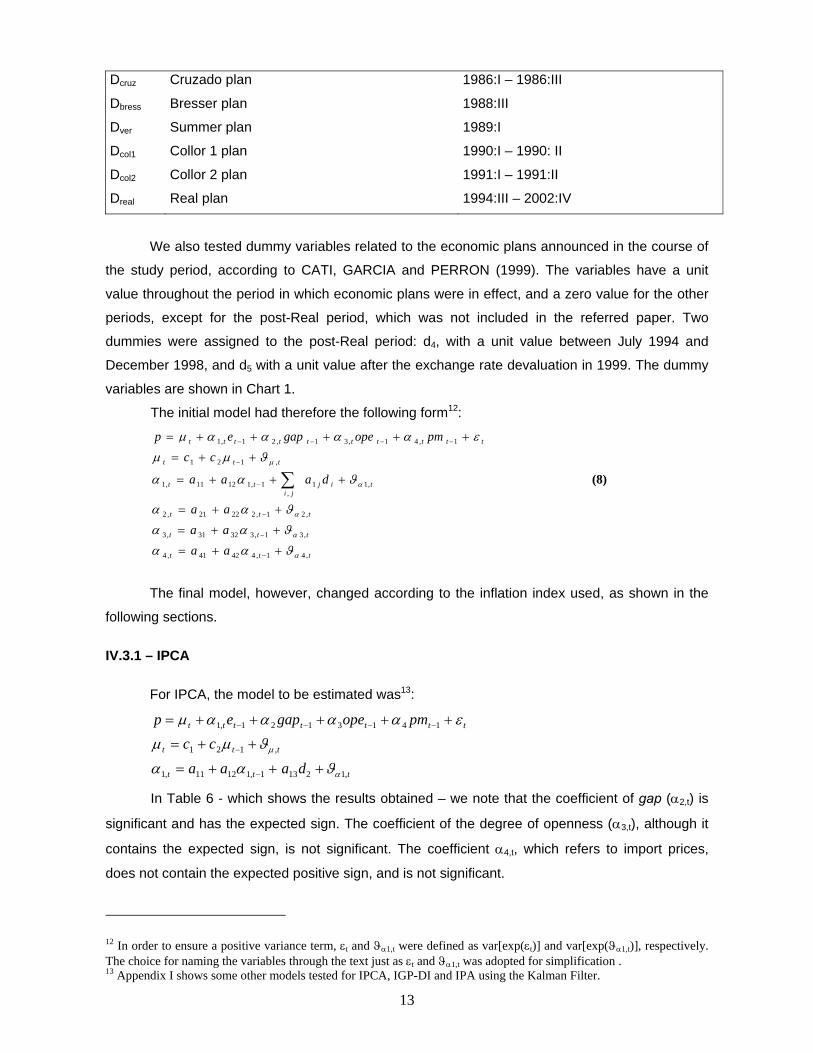
Chart 1 – Tested Dummies

Dummy Plan Period with a unit value D1 Officially floating exchange rates 1990:I – 1995:I; 1999:I – 2002:IV

D2 Managed exchange rate system 1994:III ; 1999:I – 2002:IV

D3 High inflation 1980:I – 1994:II

D4 Real Plan with pegged exchange rates 1994:III – 1998:IV

D5 Real Plan with floating exchange rates 1999:I – 2002:IV

13

Dcruz Cruzado plan 1986:I – 1986:III

Dbress Bresser plan 1988:III

Dver Summer plan 1989:I

Dcol1 Collor 1 plan 1990:I – 1990: II

Dcol2 Collor 2 plan 1991:I – 1991:II

Dreal Real plan 1994:III – 2002:IV

We also tested dummy variables related to the economic plans announced in the course of

the study period, according to CATI, GARCIA and PERRON (1999). The variables have a unit

value throughout the period in which economic plans were in effect, and a zero value for the other

periods, except for the post-Real period, which was not included in the referred paper. Two

dummies were assigned to the post-Real period: d4, with a unit value between July 1994 and

December 1998, and d5 with a unit value after the exchange rate devaluation in 1999. The dummy

variables are shown in Chart 1.

The initial model had therefore the following form12:

ttt

ttt

ttt

tijji

tt

ttt

tttttttttt

aaaaaa

daaa

ccpmopegapep

,41,44241,4

,31,33231,3

,21,22221,2

,11,

1,11211,1

,121

1,41,31,21,1

α

α

α

α

µ

ϑααϑααϑαα

ϑαα

ϑµµεααααµ

++=

++=

++=

+++=

++=

+++++=

−

−

−

−

−

−−−−

∑ (8)

The final model, however, changed according to the inflation index used, as shown in the

following sections.

IV.3.1 – IPCA

For IPCA, the model to be estimated was13:

ttt

ttt

ttttttt

daaa

ccpmopegapep

,12131,11211,1

,121

1413121,1

α

µ

ϑαα

ϑµµεααααµ

+++=

++=

+++++=

−

−

−−−−

In Table 6 - which shows the results obtained – we note that the coefficient of gap (α2,t) is

significant and has the expected sign. The coefficient of the degree of openness (α3,t), although it

contains the expected sign, is not significant. The coefficient α4,t, which refers to import prices,

does not contain the expected positive sign, and is not significant.

12 In order to ensure a positive variance term, εt and ϑα1,t were defined as var[exp(εt)] and var[exp(ϑα1,t)], respectively. The choice for naming the variables through the text just as εt and ϑα1,t was adopted for simplification . 13 Appendix I shows some other models tested for IPCA, IGP-DI and IPA using the Kalman Filter.

14

As far as variances are concerned, we note that the variances of the state equation for the

intercept and the exchange rates (ϑµ,t ϑα1,t) have significant coefficients, which means that they are

effective. In other words, the coefficients are actually varying over time and, hence, the Kalman

Filter captures changes in these coefficients that a model with constant parameters would not.

As for the intercept, we observe that c1 is not significant whereas c2 is. This means that,

although the mean of the intercept is null, shocks are persistent on it. Such a result is expected in

an inflation model if we consider that this variable captures the inflationary inertia of the period,

since the Kalman filter with varying parameters on the constant is equivalent to estimating the

stochastic trend of the series. So, we can consider that the constant, to some extent, represents

the inflationary inertia. Graph 1 shows that this coefficient becomes not only smaller but also more

stable after the implementation of the Real Plan, underscoring the idea of a remarkably low

inflationary inertia after price stabilization.

Table 6 –Kalman Filter : IPCA Results

Variable coefficient Standard error t-statistics p-value

Measure Equation

α2 1.636715 0.731031 2.238912 0.0252

α3 -0.044387 0.089447 -0.496233 0.6197

α4,t -0.001186 0.000802 -1.478920 0.1392

State Equation - Intercept

c1 0.007883 0.013579 0.580584 0.5615

c2 0.948579 0.049568 19.13699 0.0000

ϑµ,t -5.954234 0.392567 -15.16744 0.0000

State Equation – Pass-through coefficient

a11 0.489162 0.148228 3.300074 0.0010

a12 0.005248 0.188764 0.027799 0.9778

a1,3 -0.488220 0.242746 -2.011240 0.0443

ϑα1,t -2.208140 0.262412 -8.414797 0.0000

Final State Root MSE z-statistics p-value

µT+1|T 0.046336 0.065347 0.709071 0.4783

α1,T+1|T 0.001166 0.331521 0.003517 0.9972

Log-likelihood 66.15722 Akaike Information Criteria -1.225716

Hannan-Quinn Criteria -1.102508 Schwartz Information Criteria -0.920184

Concerning the behavior of the exchange rate coefficient, α1,t, a11 is significant, while a12 is

not. In the former case, the exchange rate pass-through is important in explaining prices,

regardless of the period. However, shocks on this coefficient do not propagate through time. In

other words, the stochastic process resembles a white noise. The forecast for period t+1 is given

15

by 2131,112111,1 )( daaaE tt ++= −+ αα . Since a12 and a13 are indifferent from zero, the best forecast of

the value for the exchange rate pass-through (α1,t+1) is the mean of the process, a11. Hence, an

increase of 1% in the exchange rate causes an average increase, in the period analyzed, of 0.49%

in the inflation rate. Finally, the dummy variable d2, is significant, implying that the intervention in

the exchange rate market affects the pass-through dynamics.

By analyzing Graph 2, which shows the smoothed estimates of the pass-through

coefficient, we can clearly identify three different periods in the behavior of α1. These periods may

be associated with three different moments of the Brazilian economy throughout the sample

period.

The first period goes from 1980 until the implementation of the Real plan. A considerably

high and volatile exchange rate pass–through characterizes this period, with peaks close to one,

which illustrates the exchange rate/price spiral typical of high inflations. The mean pass-through for

the period is 0.49 (see Appendix II), but there are moments of sharp reductions that may be

associated with the different economic plans (1986:II, 1987:III, 1988:IV, 1990:II, 1991:II, 1992:I).

The second period covers 1995 to 1998, where the mean drops to 0.42 (Appendix II), and

so does its volatility, showing a more stable behavior over time. Finally, the third period starts in

1999, when the floating exchange rates were adopted and the coefficient remarkably decreased,

yielding a mean value of around 0.4.

Graph 1 – IPCA: Smoothed Estimate of µ,t

- .1 .0 .1 .2 .3 .4 .5 .6

- .1 .0 .1 .2 .3 .4 .5 .6

1985 1990 1995 2000

µ t ± 2 R M S E

Graph 2 – IPCA: Smoothed Estimate of α1,t

16

-1.0

-0.5

0.0

0.5

1.0

1.5

2.0

-1.0

-0.5

0.0

0.5

1.0

1.5

2.0

1985 1990 1995 2000

α1,t ± 2 R M S E

At first, the strong decrease in 1999 is not expected since, in large devaluations, a higher

pass-through from exchange rates to prices is assumed. However, the Brazilian economic scenario

at the time, with recession and extremely volatile exchange rates, may have favored a contrary

behavior. In this scenario, price setters would not be able to increase their prices proportionately to

the devaluation as they used to do before, due to the economic slowdown, which inhibits demand,

and to the uncertainty about the future. If the exchange rates do not mantain that higher level, the

costs to reverse the price increase (menu costs and reputation costs, for instance) could be much

higher14. Furthermore, in times of pegged exchange rates, changes in exchange rates are

considered to be permanent and, therefore, agents have an extra incentive to adjust their prices as

soon as possible. However, in times of floating exchange rates, the resulting uncertainty and the

presence of factors such as menu costs and hysteresis (see DIXIT, 1986), make agents “wait and

see” until they can be sure that the (de)valuation is permanent and until they know the new

exchange rate level.

IV.3.2 – IGP-DI

The IGP-DI model is quite similar to that used for IPCA, with time-varying coefficients for

the exchange rate and intercept. Although d2 was not significant, its inclusion yielded better results

than the inclusions of other dummy variables (also nonsignificant) or than its absence. The three

periods related to the behavior of the exchange rate coefficient are more noticeable than in the

case of IPCA, and the decrease in 1999 is less intense as well, (Table 7 and graphs 3 and 4).

Table 7 Kalman Filter : IGP-DI Results

Variable Coefficient Standard error t-statistics p-value

Measurement Equation

α2 1.9712 1.0770 1.8303 0.0672

14 For a detailed ddiscussion, see DIXIT (1986).

17

α3 0.0389 0.1638 0.2377 0.8121

α4 0.0003 0.0015 0.1715 0.8638

State Equation - Intercept

c1 -5.1799 0.3117 -16.6200 0.0000

c2 0.0113 0.0200 0.5671 0.5707

ϑµ,t 0.9457 0.0414 22.8407 0.0000

State Equation - Pass-through Coefficient

a11 0.3246 0.1807 1.79645 0.0724

a12 -0.0075 0.1871 -0.0401 0.9680

a1,3 -0.2702 0.2547 -1.0611 0.2887

ϑα1,t -2.0026 0.3888 -5.1514 0.0000


µT+1|T 0.0690 0.0918 0.75120 0.4525

α1,T+1|T 0.0536 0.3674 0.1458 0.8841



As for the significance of fixed parameters and their signs, import prices are still indifferent

from zero. α2 and α3 are significant, although the former one does not present the expected sign.

With regard to the exchange rate coefficient, again, it has a white noise with drift. We may

also note that most of the sharp reductions in the coefficients are the same ones found for IPCA

(1986:II, 1987:III, 1989:I, 1989:IV, 1990:II to 1990:4, 1991:I, 1991:II, 1992:I, 1994:I). The coefficient

– or the exchange-rate elasticity of prices - is 0.3246 for the whole period. Calculating the mean of

the filtered estimates of α1,t for the three periods, we have an elasticity of 0.33 for 1980:I to 1994:II

– if we remove the above mentioned periods from the sample, this value goes to 0.40 – 0.27 from

1994:III to 1998:IV and 0.07 from 1999:I on (see Appendix II). Thus, the Real plan led to a

decrease in the pass-through, but the change in the exchange rate system and the adoption of the

inflation targeting regime in 1999 caused a sharper decrease in this coefficient.

Graph 3 – IGP-DI: Smoothed Estimate of µ,t

0.0 0.2 0.4 0.6 0.8 1.0

82 84 86 88 90 92 94 96 98 00 02 µt ± 2 R M S E

18

Graph 4 – IGP-DI: Smoothed Estimate of α1,t

-1.0 -0.5

0.0 0.5 1.0 1.5 2.0

1985 1990 1995 2000

α1,t ± 2 R M S E

Graph 5 draws some attention to the comparison of both indexes through the filtered

estimates of the exchange rate coefficients in both cases (IPCA and IGP-DI) after the Real plan.

Until 1999, the exchange rate pass-through to IPCA was, on average, higher than to the IGP-DI,

which justifies the selection of the latter one as the index used to realign contracts. After 1999, we

have an opposite situation, when the IGP-DI – which consists mostly of wholesale prices - had a

pass-through higher, on average, than that of IPCA.

Graph 5 – Filtered Estimates of α1,t for the Post-Real period: IGP-DI vs. IPCA

-0.1

0

0.1

0.2

0.3

0.4

0.5

0.6

0.7

1995

-1

1995

-2

1995

-3

1995

-4

1996

-1

1996

-2

1996

-3

1996

-4

1997

-1

1997

-2

1997

-3

1997

-4

1998

-1

1998

-2

1998

-3

1998

-4

1999

-1

1999

-2

1999

-3

1999

-4

2000

-1

2000

-2

2000

-3

2000

-4

2001

-1

2001

-2

2001

-3

2001

-4

2002

-1

2002

-2

2002

-3

2002

-4

IGPf IPCAf

IV.3.3 –IPA

The best model that the Kalman filter identified for the wholesale price index (IPA) had only

the exchange-rate coefficient as time-varying. The model assumes the following form:

ttt

tttttttttt

aapmopegapep

,11,11211,1

1,41,31,21,1

αϑαα

εααααµ

++=

+++++=

−

−−−−

19

In case of IPA, the most satisfactory results were those where only the exchange rate

coefficient varies over time. Again, α1,t follows a white noise with drift, as shown in Table 8. This

means that the best forecast for the pass-through from exchange rates to IPA is the mean of the

process. We can also note, according to Graph 6, that the only change in the behavior of the

coefficient is the peaks in the early 1990s and a smaller volatility after the Real plan. However, the

mean of the coefficient was relatively stable: 0.90 from 1980:I to 1994:II, 0.86 from 1994:3 to 98:4

and 0.87 from 1999:I on (see Appendix II). If we exclude the moments in which there was a sharp

decrease in the filtered coefficient (basically the same as with IPCA and IGP-DI: 1986:II, 1987:III,

1989:II, 1990:II, 1991:I, 1991:II, 1992:I, 1994:III, 1994:IV, 1999:II) – the mean goes to 0.93

between 1980:I and 1994:II, 0.89 for 1994:II/1998:IV and 0.88 after 1999.

The values presented here are quite high compared to the ones found for the other two

indices. As they are close to the unit, they also suggest a virtually complete pass-through from

exchange rate to wholesale prices. This result seems to demonstrate what the economic theory

had already predicted: wholesale prices are more strongly affected by exchange rate movements

and, in the absence of nontradeables, the pass-through from exchange rate to inflation is almost

complete. An explanation to this behavior can be found in the theoretical model developed in this

paper. Since Brazil is a small economy, it is a price-taker in the foreign market and it is not able to

affect international prices as predicted by the pricing-to-market models applied to developed

economies15. A smaller pass-through to consumer prices (IPCA and IGP) reflects the absorption

of the exchange rate by retailers, which can be explained – given the maximization model

presented in this paper – by an attempt to avoid a reduction in demand that is not offset by a rise in

prices. This does not necessarily mean losses for the agents, but only a change in their profit

margins.

Table 8- Kalman Filter : IPA Results

Variable Coefficient Standard error t-statistics p-value

Measure equation

µt 0.0471 0.0491 0.9590 0.3376

α2 1.9392 1.031 1.8809 0.0600

α3 -0.0937 0.2224 -0.4212 0.6736

α4 0.0019 0.0048 0.4032 0.6868

State Equation - Pass-through Coefficient

a11 1.0908 0.3694 2.9526 0.0032

a12 -0.2263 0.3667 -0.6171 0.5372

15 Those models consider that, in face of an exchange rate devaluation in country B, the exporting firm in country A will reduce its exporting prices for B in order not to have a high reduction in sales in that country, given the weight of that market on its global demand. The result of such an action is that prices in B will rise less than proportionally to the exchange rate devaluation, resulting in an incomplete pass-through and evidence of the rejection of PPP.

20

ϑα1,t -2.7168 0.9236 -2.9417 0.0033


α1, T+1|T 0.9029 0.2631 3.4323 0.0006



Graph 6 – IPA: Smoothed estimate of α2,t

0.0

0.4

0.8

1.2

1.6

0.0

0.4

0.8

1.2

1.6

1980 1985 1990 1995 2000

α2,t± 2 R M S E

21

V – Comparison of Results

According to the results obtained herein, there is a decrease in the pass-through from the

exchange rate to IPCA and IGP-DI after the stabilization of the Real, and a sharper one after the

shift in the exchange rate regime in 1999. Before 1999, the effects of an exchange rate shock in

period t on IGP-DI would be complete after approximately four quarters (considering the absence

of further shocks). After 1999, only 32% of the shock would have been absorbed by the index in an

equal period. For IPCA, between 1980 and 1998, the pass-through of the shock would be complete

in two quarters before 1999, but after that year it would represent only 7%. The exception is IPA-

DI, which keeps an almost complete pass-through in the third quarter.

The exchange rate pass-through behavior found in the present paper is in line with other

estimates reported in the literature. MINELLA, FREITAS, GOLDFAJN and MUINHOS (2003)

analyzed the post-Real period and also found a change in the exchange rate pass-through to

prices after 1999 (considering the 12-month exchange rate variation with one lag). However, the

magnitude of the change is different, depending on the approach adopted: the Central Bank’s

structural model, the Phillips curve, or a VAR model. Nonetheless, the graph of the recursive

estimation of the coefficients found in the Phillips curve for IPCA is very similar to Graph 2

presented in section IV.3.1 of this paper.

The results for IPCA in the post-Real period are also similar to the ones presented by

MUINHOS and ALVES (2003) for free prices – which correspond to approximately 70% of IPCA –

by applying a non-linear Phillips curve. The authors found an exchange rate pass-through of 0.51

between 1995:I and 1998:IV and of 0.06 from 1999:I on. The values observed for the period after

1999 are also similar to the ones presented by CARNEIRO, MONTEIRO and WU (2002), who

found a quarterly exchange rate pass-through between 1999 and 2002 of 6.4% on average.

Our results for IPCA are also close to the ones presented by BELAISCH (2003), who

observed a 6% exchange rate pass-through in Brazil in a 3-month period through a VAR model.

However, the results are considerably different for the other indices (27% for the IGP and 34% for

the IPA). Despite this difference, the relation between the magnitudes of the coefficients is the

same: the pass-through to IPA is larger than to IGP, which is larger than to IPCA.

GODLJAN and WERLANG (2000) found a six-month accumulated pass-through of about

21% for European economies and 38% for emerging ones between 1980 and 1998. HAUSSMAN,

PANIZZA and STEIN (1999) also encountered different pass-through values among the analyzed

countries. For instance, the USA, the UK and Japan have an average 12-month accumulated

pass-through of 3%; Germany, Canada and Norway, 7%; Switzerland, Greece, Israel and Korea,

16%; Australia and Peru, 21%, and Mexico, Paraguay and Poland, over 50%, among others.

MUINHOS (2001) uses a sample with quarterly data from 1980 to 2000, different

estimations of the Phillips curve, with and without an expectation term and with linear and non-

linear specifications (the latter of which contains cross-terms), also including a short sample

22

relating to the period after 1995. The results of the linear specification point towards a pass-

through coefficient of 0.10 in the small sample if the expectation term is not included and of 0.09 if

this term is included. In the non-linear specification, the pass-through coefficients are 0.24 without

the expectation term, 0.12 with the term, and 0.55 for the whole sample. However, the results do

not indicate changes in the exchange rate pass-through after 1995 in the whole sample, or in both

samples, after 1999. When the authors show the behavior of pass-through coefficients after 1998

for the small sample, there is a break in this coefficient after the floating exchange rate regime was

adopted. The average coefficient for 1998 is, in this case, higher than 0.5 while it is of about 0.1

after 1999, a result that is in line with the ones presented in this paper. Nevertheless, such change

is not identified in the whole sample (1980 to 2000) when the coefficient for 1998 is also around

0.1.

VI – Final Remarks

Some conclusions may be drawn in light of what was discussed in this paper. The first

conclusion is that the model developed from a pricing-to-market approach is able to indicate

changes that occurred in the exchange rate coefficient throughout the study period. Furthermore,

amongst the tested formulations, non-linear models and time-variant coefficients are more suitable

than OLS coefficients with time-invariant parameters, even when the sample is divided. The results

obtained by MUINHOS (2001) who, as other previously mentioned authors, observed a decrease

in the exchange rate pass-through after 1999 only when using the small sample, lends further

support to the Kalman Filter to the detriment of time-invariant models, when such a long and

complex period is analyzed.

In comparison with the results found by GOLDFJAN and WERLANG (2000) and by

HAUSSMAN, PANIZZA and STEIN (1999), the data presented herein show that the pass-through

from the exchange rate to prices in Brazil is not only smaller after the adoption of the floating

exchange rate system in 1999, but also quite similar to the ones observed in stronger economies.

Our paper shows that the macroeconomic environment affects the way prices will respond to

exchange rate movements, as it is possible to identify three different patterns in the pass-through

coefficient: the first one is characterized by a high inflation period, the second one concerns the

period of low inflation and pegged exchange rates, and the third one refers to the period of stable

prices and floating exchange rates. The presence of the dummy variable d2 also suggests that the

type of exchange rate regime observed by the agents – more than the one officially announced –

also affects the response of prices to exchange rate movements.

23

References AMITRANO, A.; de GRAUWE, P.; TULLIO, G. (1997) Why has inflation remained so low after the

long exchange rate depreciations of 1992?, Journal of common market studies, vol. 35, n.3,

September

ANDERSEN, T. M. (1997) Exchange rate volatility, nominal rigidities and persistent deviations from

PPP, Journal of the Japanese and International Economies, 11, pp. 584-609

ARAUJO, C.H.V.; FILHO, G.B.S. (2002) Mudanças de regime no câmbio brasileiro, Central Bank

of Brazil, working paper no. 41, June

BELAISCH, Agnes (2003) Exchange rate pass-through in Brazil, IMF working papers, n. 141, July

BETTS, C.; DEVEREAUX, M. B. (2000), Exchange rate dynamics in a model of pricing-to-market,

Journal of Monetary Economics, 50, pp. 215-244

BOGDANSKI, J.; TOMBINI, A.A.; WERLANG, S.R.C., (2000) Implementing inflation targeting in

Brazil, Banco Central do Brasil, working paper no. 1, July

BORENSZTEIN, E.; de GREGORIO, J. (1999) Devaluation and inflation after currency crisis,

mimeo, February

CALVO, G; REINHART, C. (2000) Fixing for your life, NBER, working paper no. 8006, November

CARNEIRO,D.; MONTEIRO, A.M.D., WU, T.Y.H. (2002) Mecanismos não-lineares de repasse

cambial para o IPCA, PUC-RIO, working paper no. 462, August

CATI, R. C.; GARCIA, M G P; PERRON, P. (1999). Unit Roots in the Presence of Abrupt

Governmental Interventions with an Application to Brazilian Data, Journal of Applied

Econometrics, Vol. 14 (1) pp. 27-56.

DIXIT, A. (1989) Hysteresis, import penetration, and exchange rate pass-through, The Quarterly

Journal of Economics, CIV, pp. 205-228, May

DORNBUSCH, R. (1976) Expectations and exchange rate dynamics, Journal of Economic

Literature, v. 84, n.6, pp.1161-76, December

EICHENGREEN, B. (2002) Can emerging markets float the way they float? Should they inflation

target?, Central Bank of Brazil, working paper no. 36, February

FEENSTRA,R.C.; KENDAL, J.D. (1997) Pass-through of exchange rates and purchasing power

parity, Journal of International Economics, 43, pp. 237 – 261

FIGUEIREDO, F.M.R.; FERREIRA, T. P. (2002) Os preços administrados e a inflação no Brasil,

Central Bank of Brazil, working paper, Brasília, no. 59, December

FIORENCIO, A.; MOREIRA, A.R.B. (1999) Latent indexation and exchange rate pass-through

IPEA, Rio de Janeiro: working paper no. 650, July

FISHER, ERIC (1989) A model of exchange rate pass-through, Journal of International Economics,

26, pp. 119-137

FRANKEL, J. A. (1978) Purchasing Power Parity: doctrinal perspective and evidence from the

1920s, Journal of International Economy, 8 (2), pp. 169-91, May

24

GOLDBERG, P. K.; KNETTER, M. M.; (1996) Goods prices and exchange rates: what have we

learned? NBER, working paper no. 5862, December

GOLDFJAN, I.; WERLANG, S.R.C. (2000) The pass-through from depreciation to inflation: a panel

study, Banco Central do Brasil, working paper no. 5, September

HAUSSMANN, R.; PANIZZA, U.;STEIN, E. (1999) Why do countries float the way they float?,

working paper no. 418, Inter-American Development Bank (BIRD)

KIMBROUGH, K.P., (1983), Price, output and exchange rate movements in the open economy,

Journal of Monetary Economics, 11, pp. 25 - 44

KLAASSEN, F. (1999) Purchasing Power Parity: Evidence from a new test, Tilburg University,

CentER and Department of Economics, January

KLEIN, M. W. (1990) Macroeconomics aspects of exchange rate pass-through, Journal of

international money and finance, 9, pp. 376 – 387

KRUGMAN, P. (1986) Pricing to market when the exchange rate changes, NBER, working paper

no. 1926, May

KRUGMAN, P. (1988); Exchange Rate Instability, Cambridge, MA: The MIT press

LEIDERMAN, L., BAR-OR, H. (2000), H. Monetary policy rules and transmission mechanisms

under inflation targeting in Israel, Banco Central de Chile, documentos de trabajo, n. 71, May

LOSCHIAVO, G.V.; IGLESIAS, C.V. (2002) Mecanismos de transmisión de la política monetario-

cambiaria a precios, Banco Central del Uruguay, Decimaséptimas Jornadas Anuales de

Economía; 26, July

MINELLA, A.; FREITAS, Paulo S.; GODLFAJN, Ilan; MUINHOS, M.K. (2003), Inflation targeting in

Brazil: lessons and challenges, Banco Central do Brasil, working paper no. 53, November

MUINHOS, Marcelo K. (2001) Inflation Targeting in an open financially integrated emerging

economy: the case of Brazil, Banco Central do Brasil, working paper no. 26, August

MUINHOS, Marcelo K.; ALVES, Sérgio A. L. (2003) Medium-size macroeconomic model for the

Brazilian economy, Banco Central do Brasil, working paper no. 64, February

OBSTFELD, M; ROGOFF, K. (2000) The six major puzzles in international macroeconomics: is

there a common cause?, NBER, working paper no. 7777, July

PARSLEY D. (1995) Anticipated future shocks and exchange rate pass-through in the presence of

reputation, International Review of Economics and Finance, 4(2): 99-103

ROGOFF, K. (1996) The purchasing power parity puzzle, Journal of Economic Literature, 34, pp.

647 - 68 , June

ROMER, D. (1993) Openness and inflation: theory and evidence, The Quarterly Journal of

Economics, CVIII, pp. 869-903, November

ROMER, D. (1998), A New Assessment of Openness and Inflation: Reply, "The Quarterly Journal

of Economics, n. 113, pp. 649-652, May

SMITH, C. E. (1999) Exchange rate variation, commodity price variation and the implications for

international trade, Journal of International Money and Finance, 18, pp, 471– 491

25

TAYLOR, J. B.(2000) Low inflation, pass-through, and the pricing power of firms, European

Economic Review¸44, pp.1389 – 1408

TERRA, C.T. (1998) Openness and inflation: a new assessment, The Quarterly Journal of

Economics, n. 113, pp. 641-648, May

VIANE, J.M.; de VRIES, C. G. (1992) International trade and exchange rate volatility, European

Economic Review, 36, pp. 1311 - 1321

26

APPENDIX I – LINEAR MODEL RESULTS

A.I – Linear Models – Complete Sample (TABLES) Table A.1 - IPCA

Coefficient Estimate Standard Error t-statistics p-value

µ 0.0508 0.0286 1.7784 0.0789 α1 0.8398 0.0684 12.2763 0.0000 α2 2.1079 0.7436 2.8349 0.0057 α3 -0.3304 0.1884 -1.7534 0.0831 α4 -0.0007 0.0037 -0.1965 0.8447

R2 0.6433 Mean dependent var 0.2891 R2 adjusted 0.6265 S.D. dependent var 0.3205 S.E. of regression 3.2603 AIC -0.3690 LM test (1st order) 0.0065† SIC -0.2301 ARCH-LM test (1st order) 17.6433* F-statistic 38.3271 Ramsey-Reset test (2nd order) 2.9960* Prob(F-statistic) 0.0000

* significant at 5%;† for higher orders the presence of residual autocorrelation was also rejected

Table A.2 – IGP-DI


µ 0.0644 0.0290 2.2220 0.0289 α1 0.8083 0.0695 11.6346 0.0000 α2 1.9492 0.7552 2.5812 0.0116 α3 -0.1666 0.1914 -0.8703 0.3866 α4 0.0008 0.0038 0.1975 0.8439

R2 0.6152 Mean dependent var 0.2955 R2 adjusted 0.5971 S.D. dependent var 0.3134 S.E. of regression 0.1989 AIC -0.3380 LM test (1st order) 2.5224** SIC -0.1991 ARCH-LM test (1st order) 0.5579† F-statistic 33.9716 Ramsey-Reset test (1st order) 3.4552* Prob(F-statistic) 0.0000

* significant at 5%; ** significant at 10%;† for higher orders the presence of residual autocorrelation was also rejected

Table A.3 – IPA


µ 0.0636 0.0292 2.1778 0.0322 α1 0.8119 0.0699 11.6112 0.0000 α2 1.9018 0.7600 2.5024 0.0143 α3 -0.1830 0.1926 -0.9504 0.3446 α4 0.0008 0.0038 0.2105 0.8338

R2 0.6145 Mean dependent var 0.2955 R2 adjusted 0.5964 S.D. dependent var 0.3151 S.E. of regression 0.2002 AIC -0.3252 LM test (2st order) 3.2633* SIC -0.1863 ARCH-LM test (2nd order) 5.6300* F-statistic 33.8757 Ramsey-Reset test (1st order) 3.5620* Prob(F-statistic) 0.0000

* significant at 5%

27

A.II – Alternative Linear Models (TABLES) Table A.4 – IPCA

Coefficient Pre-Real Post-Real Model with dummy variables

µ 0.1415* (0.0516)

0.0173* (0.0032)

0.0554 (0.0269)**

α1 0.7262* (0.1077)

0.0568 (0.0355)

0.8888 (0.0655)*

α14 - - -0.5680* (0.1669)

α15 - - -0.8551** (0.3792)

α2 2.4121* (0.9129)

0.4505* (0.1683)

2.17881* (0.0022)

α3 -0.1325 (0.2798)

-0.0125 (0.0265)

-0.1591 (0.1824)

α4 -0.0012 (0.0054)

0.0005 (0.0005)

-0.0008 (0.0035)

R2 0.4888 0.2304 0.7006 R2 adjusted 0.4471 0.1164 0.6789 S.E. of regression 2.3945 0.0147 0.1816 LM test (1st order) 0.0879† 13.5814* 0.7835† ARCH-LM test (1st order) 7.8165* 6.5385* 23.0965* Ramsey-Reset test (1st order) 2.9151***(a) 0.2304**

*significant at 1%; **significant at 5%; ***significant at 10%; (a) test in second order; † for higher orders, residual

autocorrelation was also rejected

Table A.5 – IGP-DI


µ 0.1808* (0.0526)

0.0222* (0.0042)

0.0707* (0.0282)

α1 0.6341* (0.1097)

0.0876** (0.04551)

0.8428 (0.0686)*

α14 - - -0.4192* (0.1748)

α15 - - -0.8658** (0.3971)

α2 2.2269* (0.9301)

0.0186 (0.21571)

1.9876 (0.7234)

α3 0.0843 (0.2851)

0.0351 (0.0340)

-0.0184 0.0394)

α4 0.0006 (0.0055)

0.0010 (0.006)

-0.0003 (0.0008)

R2 0.4210 0.2655 0.6564 R2 adjusted 0.3737 0.1567 0.6316 S.E. of regression 0.2252 0.0189 0.1902 LM test (1st order) 4.2357(a) ** 0.3868† 1.3723 ** ARCH-LM test (1st order) 0.0830† 0.6568† 1.4793** Ramsey-Reset test (1st order) 2.3705(a)*** 3.6850**(a) 0.6564

*significant at 1%; **significant at 5%; ***significant at 10%; (a) test in second order; † for higher orders, residual

autocorrelation was also rejected

28

Table A.6– IPA-DI


µ 0.1721* (0.0536)

0.0252* (0.0055)

0.0688* (0.0284)

α1 0.6562* (0.1112)

0.1023*** (0.0617)

0.8483* (0.0692)

α14 - - -0.4344* (0.1764)

α15 - - -0.7943** (0.4007)

α2 2.2346* (0.9468)

-0.3548 (0.2924)

1.9477* (0.7299)

α3 0.0242 (0.2902)

0.0599 (0.0461)

-0.0342 (0.1928)

α4 0.0006 (0.0056)

0.0011 (0.0009)

0.0007 (0.0037)

R2 0.4256 0.324 0.6541 R2 adjusted 0.3787 0.2239 0.6291 S.E. of regression 0.2293 0.0256 0.1919 LM test (1st order) 3.9428**(a)

0.0117† 2.4383†

ARCH-LM test (1st order) 4.6245**(a) 3.4787***(a) 4.4998** Ramsey-Reset test (1st order) 2.8311*** 6.4948**(a)

*significant at 1%; **significant at 5%; ***significant at 10%; (a) test in second order; † for higher orders, residual autocorrelation was also rejected

A.I – Linear Models (GRAPHS) Graph A.1– IPCA – CUSUM of Squares test (complete period)

-0.2

0.0

0.2

0.4

0.6

0.8

1.0

1.2

82 84 86 88 90 92 94 96 98 00 02

C U S U M o f S q u a r e s 5 % S i g n i f i c a n c e

Graph A.2 – IPCA – Recursive Coefficients (complete period)

- . 2 - . 1 . 0 . 1 . 2 . 3

8 4 8 6 8 8 9 0 9 2 9 4 9 6 9 8 0 0 0 2 E s t i m a t i v a s r e c u r s i v a s d e µ ± 2 S . E .

- 0 . 4

0 . 0

0 . 4

0 . 8

1 . 2

1 . 6

8 4 8 6 8 8 9 0 9 2 9 4 9 6 9 8 0 0 0 2

E s t i m a t i v a s r e c u r s i v a s d e α 1 -± 2 S . E .

- 1

0

1

2

3

4

5

8 4 8 6 8 8 9 0 9 2 9 4 9 6 9 8 0 0 0 2

E s t i m a t i v a s r e c u r s i v a s d e α 2

± 2 S . E .

- 1 . 2 - 0 . 8 - 0 . 4 0 . 0 0 . 4 0 . 8

8 4 8 6 8 8 9 0 9 2 9 4 9 6 9 8 0 0 0 2 E s t i m a t i v a s r e c u r s i v a s d e α 3 ± 2 S . E .

- . 0 1 5

- . 0 1 0

- . 0 0 5

. 0 0 0

. 0 0 5

. 0 1 0

. 0 1 5

8 4 8 6 8 8 9 0 9 2 9 4 9 6 9 8 0 0 0 2

E s t i m a t i v a s r e c u r s i v a s d e α 4

± 2 S . E .

29

Graph A.3 – IPCA – CUSUM of Squares test (pre-Real period)

-0.4

0.0

0.4

0.8

1.2

1.6

1982 1984 1986 1988 1990 1992


Graph A.4 – IPCA - Recursive Coefficients (pre-Real period)

-.2 -.1 .0 .1 .2 .3 .4

83 84 85 86 87 88 89 90 91 92 93 E s t i m a t i v a s r e c u r s i v a s d e µ ± 2 S . E .

-1.0 -0.5

0.0 0.5 1.0 1.5

83 84 85 86 87 88 89 90 91 92 93

E s t i m a t i v a s r e c u r s i v a s d e α1

± 2 S . E .

-2

-1

0

1

2

3

4

5

83 84 85 86 87 88 89 90 91 92 93

E s t i m a t i v a s r e c u r s i v a s d e α2 ± 2 S . E .

-.8 -.6 -.4 -.2 .0 .2 .4 .6 .8

83 84 85 86 87 88 89 90 91 92 93 E s t i m a t i v a s r e c u r s i v a s d e α3 ± 2 S . E .

-.015 -.010 -.005 .000 .005 .010 .015

83 84 85 86 87 88 89 90 91 92 93

E s t im a t i v a s r e c u r s iv a s d e α4

± 2 S . E .

Graph A.5 – IPCA - CUSUM of Squares Test (post-Real period)

- 0 . 4

0 . 0

0 . 4

0 . 8

1 . 2

1 . 6

1 9 9 6 1 9 9 7 1 9 9 8 1 9 9 9 2 0 0 0 2 0 0 1 2 0 0 2


Graph A.6 – IPCA - Recursive Coefficients (post-Real period)

.00

.01

.02

.03

.04

.05

.06

.07

1998 1999 2000 2001 2002

R e c u r s i v e C ( 1 ) E s t i m a t e s ± 2 S . E .

-1.2

-1.0

-0.8

-0.6

-0.4

-0.2

0.0

0.2

1998 1999 2000 2001 2002


-0.4

-0.2

0.0

0.2

0.4

0.6

0.8

1.0

1.2

1998 1999 2000 2001 2002

R e c u r s iv e C ( 3 ) E s t im a t e s ± 2 S . E .

-.08

-.04

.00

.04

.08

.12

1998 1999 2000 2001 2002


-.004

.000

.004

.008

.012

.016

.020

.024

1998 1999 2000 2001 2002


30

Graph A.7 – IPCA - CUSUM of SquaresTest - model with dummy variables

-0.4

0.0

0.4

0.8

1.2

1.6

99:1 99:3 00:1 00:3 01:1 01:3 02:1 02:3


Graph A.8 – IPCA - Recursive Coefficients - model with dummy variables

-.02 .00 .02 .04 .06 .08 .10 .12 .14

00:4 01:1 01:2 01:3 01:4 02:1 02:2 02:3 02:4 E s t i m a t i v a r e c u r s i v a d e µ ± 2 S . E .

0.70

0.75

0.80

0.85

0.90

0.95

1.00

1.05

00:4 01:1 01:2 01:3 01:4 02:1 02:2 02:3 02:4

E s t i m a t i v a r e c u r s iva

a d e α1 ± 2 S . E .

-1.0

-0.9

-0.8

-0.7

-0.6

-0.5

-0.4

-0.3

-0.2

00:4 01:1 01:2 01:3 01:4 02:1 02:2 02:3 02:4

E s t i m a t i v a r e c u r s i v a d e α14 ± 2 S . E .

-2.0 -1.6 -1.2 -0.8 -0.4

0.0 0.4

00:4 01:1 01:2 01:3 01:4 02:1 02:2 02:3 02:4 E s t i m a t i v a r e c u r s i v a d e α15 ± 2 S . E .

0.5

1.0

1.5

2.0

2.5

3.0

3.5

4.0

00:4 01:1 01:2 01:3 01:4 02:1 02:2 02:3 02:4

E s t i m a t i v a r e c u r s i v a de α2 ± 2 S . E .

-.6

-.5

-.4

-.3

-.2

-.1

.0

.1

.2

.3

00:4 01:1 01:2 01:3 01:4 02:1 02:2 02:3 02:4

E s t i m a t i v a r e c u r s i v a d e α3 ± 2 S . E .

-.012 -.008 -.004

.000

.004

.008

.012

00:4 01:1 01:2 01:3 01:4 02:1 02:2 02:3 02:4 E s t i m a t i v a r e c u r s i v a d e α4 ± 2 S . E .

Graph A.9 – IGP - CUSUM of Squares test (complete period)

-0 .2

0 .0

0 .2

0 .4

0 .6

0 .8

1 .0

1 .2

8 2 8 4 8 6 8 8 9 0 9 2 9 4 9 6 9 8 0 0 0 2

C U S U M o f S q u a re s 5 % S ig n if ic a n c e

Graph A.10 – IGP - Recursive Coefficients (complete period)

-.1 .0 .1 .2 .3 .4

84 86 88 90 92 94 96 98 00 02 E s t i m a t i v a r e c u r s i v a d e µ t

± 2 S . E .

0.0

0.2

0.4

0.6

0.8

1.0

1.2

1.4

1.6

84 86 88 90 92 94 96 98 00 02Es tim ativa re c u rs iva do c oe f ic ie n te de α1

± 2 S . E .

-2

-1

0

1

2

3

4

5

84 86 88 90 92 94 96 98 00 02

Es tim ativa rec u r s i v a d o c o e f i c i e n t e d e α2 ± 2 S .E .

-0.8 -0.4 0.0 0.4 0.8 1.2

84 86 88 90 92 94 96 98 00 02 E s t i m a t i v a r e c u r s i v a d o c oe f i c i e n t e d e α3 ± 2 S . E .

-.012

-.008

-.004

.000

.004

.008

.012

.016

.020

84 86 88 90 92 94 96 98 00 02

Estim ativa re c u rs iva do c oef ic ie nte de α4

± 2 S .E .

31

Graph A.11 – IGP - CUSUM of Squares test (pre-Real period)

-0 .4

0 .0

0 .4

0 .8

1 .2

1 .6

1 9 8 2 1 9 8 4 1 9 8 6 1 9 8 8 1 9 9 0 1 9 9 2


Graph A.12 – IGP - Recursive Coefficients (pre-Real period)

- .1 .0 .1 .2 .3 .4

8 3 8 4 8 5 8 6 8 7 8 8 8 9 9 0 9 1 9 2 9 3 E s t i m a t i v a s r e c u r s i v a s d e µ t ± 2 S . E .

- 1 .5

- 1 .0

- 0 .5

0 .0

0 .5

1 .0

1 .5

8 3 8 4 8 5 8 6 8 7 8 8 8 9 9 0 9 1 9 2 9 3

E s t im a ti v a s r e c u r s iv a s d e α 1 ± 2 S . E .

- 2

- 1

0

1

2

3

4

5

8 3 8 4 8 5 8 6 8 7 8 8 8 9 9 0 9 1 9 2 9 3

E s t i m a t i v a s r e c u r s i v a s d e α 2 ± 2 S . E .

- 0 .6 - 0 .4 - 0 .2 0 .0 0 .2 0 .4 0 .6 0 .8 1 .0

8 3 8 4 8 5 8 6 8 7 8 8 8 9 9 0 9 1 9 2 9 3 E s t i m a t i v a s r e c u r s i v a s d e α 3 ± 2 S . E .

- .0 1 2

- .0 0 8

- .0 0 4

.0 0 0

.0 0 4

.0 0 8

.0 1 2

.0 1 6

.0 2 0

8 3 8 4 8 5 8 6 8 7 8 8 8 9 9 0 9 1 9 2 9 3

E s t i m a t i va s r e c u r s i va s d eα 4 ± 2 S . E .

Graph A.13 – IGP - CUSUM of Squares Test (post-Real period)

-0 .4

0 .0

0 .4

0 .8

1 .2

1 .6

1 9 9 6 1 9 9 7 1 9 9 8 1 9 9 9 2 0 0 0 2 0 0 1 2 0 0 2


Graph A.14 – IGP Recursive Coefficients (post-Real period)

-.01 .00 .01 .02 .03 .04 .05

1998 1999 2000 2001 2002 E s t i m a t i v a r e c u r s i v a d e µ ± 2 S . E .

-0.8

-0.4

0.0

0.4

0.8

1.2

1998 1999 2000 2001 2002

E s ti m a t i va r e c u r s i va de α1 ± 2 S . E .

-0.8

-0.4

0.0

0.4

0.8

1.2

1998 1999 2000 2001 2002

E s ti m a t i v a r e c u r s i v a d e α2 ± 2 S . E .

-.08 -.04 .00 .04 .08 .12

1998 1999 2000 2001 2002 E s t i m a t i v a r e c u r s i v a d e α3 ± 2 S . E .

-.008

-.004

.000

.004

.008

.012

.016

1998 1999 2000 2001 2002

E s ti m a ti va r e c u r s iv a d e α4 ± 2 S . E .

32

Graph A.15 – IGP - CUSUM of SquaresTest - model with dummy variables

-0 .4

0 .0

0 .4

0 .8

1 .2

1 .6

9 9 :1 9 9 :3 0 0 :1 0 0 :3 0 1 :1 0 1 :3 0 2 :1 0 2 :3


Graph A.16 – IGP - Recursive Coefficients - model with dummy variables

.00 .02 .04 .06 .08 .10 .12 .14 .16

00:4 01:1 01:2 01:3 01:4 02:1 02 :2 02:3 02:4 E s t i m a t i v a r e c u r s i v a d e µ ± 2 S . E .

0.68

0.72

0.76

0.80

0.84

0.88

0.92

0.96

1.00

00 :4 01:1 01:2 01:3 01:4 02:1 02 :2 02:3 02:4

E s t i m a t i v a r e c u r s i v a de α 1 ± 2 S . E .

-.8

-.7

-.6

-.5

-.4

-.3

-.2

-.1

.0

00:4 01:1 01 :2 01:3 01:4 02 :1 02:2 02 :3 02:4

E s t i m a t i v a r e c u r s i v a de α 14 ± 2 S . E .

-2.0 -1.6 -1.2 -0.8 -0.4

0.0 0.4

00:4 01 :1 01:2 01:3 01:4 02 :1 02 :2 02 :3 02:4 E s t i m a t i v a r e c u r s i v a d e α 15 ± 2 S . E .

0.0

0 .5

1 .0

1 .5

2 .0

2 .5

3 .0

3 .5

4 .0

00 :4 01:1 01:2 01:3 01:4 02:1 02 :2 02:3 02:4

E s t i m a t i v a r e c u r s i v a d e α 2 ± 2 S . E .

-.6

-.4

-.2

.0

.2

.4

.6

00:4 01:1 01 :2 01:3 01:4 02 :1 02:2 02 :3 02:4

E s t i m a t i v a r e c u r s i v a d e α 3 ± 2 S . E .

-.012 -.008 -.004

.000

.004

.008

.012

00:4 01:1 01:2 01:3 01:4 02:1 02 :2 02:3 02:4 E s t i m a t i v a r e c u r s i v a d e α 4 ± 2 S . E .

Graph A.17 – IPA - CUSUM of Squares test (complete period)

-0.2

0.0

0.2

0.4

0.6

0.8

1.0

1.2

82 84 86 88 90 92 94 96 98 00 02


Graph A.18 – IPA - Recursive Coefficients (complete period)

-.1 .0 .1 .2 .3

84 86 88 90 92 94 96 98 00 02 e s t i m a t i v a r e c u r s i v a d e µ ± 2 S . E .

0.0

0.4

0.8

1.2

1.6

2.0

84 86 88 90 92 94 96 98 00 02

e s t im a t iv a r e c u rs iv a d o c o e f ic i e n t e d e α1

± 2 S . E .

-2

-1

0

1

2

3

4

5

84 86 88 90 92 94 96 98 00 02 e s t im a t iv a r e c u r s iv a d o c o e f i c i e n t e d e α2

± 2 S . E .

-.8 -.4 .0 .4 .8

84 86 88 90 92 94 96 98 00 02 e s t i m a t i v a r e c u r s i v a d o c o e f i c i e n t e d e α3 ± 2 S . E .

-.012

-.008

-.004

.000

.004

.008

.012

.016

.020

84 86 88 90 92 94 96 98 00 02

e s t i m a t i v a re c u rs i v a d o c o e f ic ie n t e d e α4

± 2 S . E .

33

Graph A.19 – IPA - CUSUM of Squares test (pre-Real Period)

- 0 . 4

0 . 0

0 . 4

0 . 8

1 . 2

1 . 6

1 9 8 2 1 9 8 4 1 9 8 6 1 9 8 8 1 9 9 0 1 9 9 2


Graph A.20 – IPA - Recursive Coefficients (pre-Real period)

-.1 .0 .1 .2 .3 .4 .5

83 84 85 86 87 88 89 90 91 92 93 E s t i m a t i v a s r e c u r s i v a s d e µ ± 2 S . E .

-1.5 -1.0 -0.5 0.0 0.5 1.0 1.5 2.0

83 84 85 86 87 88 89 90 91 92 93

E s t i m a t i v a s r e c u r s iv a s d o c o e f i c ie n t e d e α1

± 2 S . E .

-2

-1

0

1

2

3

4

5

83 84 85 86 87 88 89 90 91 92 93

E s t i m a t iv a s r e c u r s i v a s d o c o e f i c i e n t e d e α2

± 2 S . E .

-.8 -.6 -.4 -.2 .0 .2 .4 .6 .8

83 84 85 86 87 88 89 90 91 92 93 E s t i m a t i v a s r e c u r s i v a s d o c o e f i c i e n t e d e α3 ± 2 S . E .

-.012 -.008 -.004 .000 .004 .008 .012 .016 .020

83 84 85 86 87 88 89 90 91 92 93

E s t im a t i v a s r e c u r s i v a s d o c o e f i c i e n t e d e α4

± 2 S . E .

Graph A.22 – IPA - CUSUM of Squares Test (post-Real period)

- 0 . 4

0 . 0

0 . 4

0 . 8

1 . 2

1 . 6

1 9 9 6 1 9 9 7 1 9 9 8 1 9 9 9 2 0 0 0 2 0 0 1 2 0 0 2


Graph A.23 - IPA –Recursive Coefficients (post-Real period)

-.02 -.01 .00 .01 .02 .03 .04 .05 .06

1998 1999 2000 2001 2002 E s t i m a t i v a r e c u r s i v a d e µ ± 2 S . E .

-1.0 -0.5 0.0 0.5 1.0

1998 1999 2000 2001 2002

E s t im a t i va r e c u r s iv a d o c o e f i c i e n te d e α1± 2 S . E .

-1.2

-0.8

-0.4

0.0

0.4

0.8

1998 1999 2000 2001 2002 E s t i m a ti va r e c u r s i v a d o c o e f i c i e n t e d e α2 ± 2 S . E .

-.10 -.05

.00

.05

.10

.15

.20

1998 1999 2000 2001 2002 E s t i m a t i v a r e c u r s i v a d o c o e f i c i e n t e d e α3 ± 2 S . E .

-.010 -.005 .000 .005 .010 .015 .020

1998 1999 2000 2001 2002

E s t i m a t iv a r e c u r s i va d o c o e f ic i e n te d e α4

± 2 S . E .

34

Graph A.24 – IPA - CUSUM of SquaresTest - model with dummy variables

- 0 . 4

0 . 0

0 . 4

0 . 8

1 . 2

1 . 6

9 9 : 1 9 9 : 3 0 0 : 1 0 0 : 3 0 1 : 1 0 1 : 3 0 2 : 1 0 2 : 3


Graph A.25 – IPA - Recursive Coefficients - model with dummy variables

.00 .02 .04 .06 .08 .10 .12 .14

00:4 01:1 01:2 01:3 01:4 02:1 02:2 02:3 02:4 E s t i m a t i v a r e c u r s i v a de µ ± 2 S . E .

0.68 0.72 0.76 0.80 0.84 0.88 0.92 0.96 1.00

00:4 01:1 01:2 01:3 01:4 02:1 02:2 02:3 02:4


-.9

-.8

-.7

-.6

-.5

-.4

-.3

-.2

-.1

.0

00:4 01:1 01:2 01:3 01:4 02:1 02:2 02:3 02:4


-2.0 -1.6 -1.2 -0.8 -0.4 0.0 0.4

00:4 01:1 01:2 01:3 01:4 02:1 02:2 02:3 02:4 E s t i m a t i v a r e c u r s i v a de α15 ± 2 S . E .

0.0 0.5 1.0 1.5 2.0 2.5 3.0 3.5 4.0

00:4 01:1 01:2 01:3 01:4 02:1 02:2 02:3 02:4


-.5

-.4

-.3

-.2

-.1

.0

.1

.2

.3

.4

00:4 01:1 01:2 01:3 01:4 02:1 02:2 02:3 02:4


-.012 -.008 -.004 .000 .004 .008 .012

00:4 01:1 01:2 01:3 01:4 02:1 02:2 02:3 02:4 E s t i m a t i v a r e c u r s i v a de α4 ± 2 S . E .

35

APPENDIX II – FILTERED COEFFICIENTS– VALUES AND MEANS

II.1 – Filtered Coefficients of α1,t – IPCA

DATE Coefficient Filtered Estimate DATE Coefficient

Filtered Estimate DATE Coefficient Filtered Estimate

1980-1 0.0000 1987-4 0.3051 1995-3 0.5409 1980-2 0.4582 1988-1 0.7671 1995-4 0.4747 1980-3 0.4620 1988-2 0.4572 1996-1 0.4550 1980-4 0.5130 1988-3 1.4162 1996-2 0.4481 1981-1 0.3686 1988-4 -0.4444 1996-3 0.4612 1981-2 0.4391 1989-1 0.6641 1996-4 0.4225 1981-3 0.5050 1989-2 0.7343 1997-1 0.4624 1981-4 0.5096 1989-3 0.8732 1997-2 0.4543 1982-1 0.6443 1989-4 0.6297 1997-3 0.4541 1982-2 0.4166 1990-1 1.0293 1997-4 0.4454 1982-3 0.3926 1990-2 0.1772 1998-1 0.4643 1982-4 0.3397 1990-3 0.1075 1998-2 0.4717 1983-1 0.6340 1990-4 0.2846 1998-3 0.4367 1983-2 0.4925 1991-1 0.4021 1998-4 0.4646 1983-3 0.5250 1991-2 0.1042 1999-1 0.0819 1983-4 0.5661 1991-3 0.4583 1999-2 0.0197 1984-1 0.5688 1991-4 0.4620 1999-3 0.0378 1984-2 0.5024 1992-1 0.1729 1999-4 0.0218 1984-3 0.5192 1992-2 0.3231 2000-1 0.0034 1984-4 0.5487 1992-3 0.3244 2000-2 0.1217 1985-1 0.4631 1992-4 0.5412 2000-3 0.0393 1985-2 0.2699 1993-1 0.5287 2000-4 0.0208 1985-3 0.4645 1993-2 0.4926 2001-1 -0.0557 1985-4 0.5364 1993-3 0.5694 2001-2 0.0342 1986-1 0.4541 1993-4 0.6168 2001-3 0.0422 1986-2 -0.1555 1994-1 0.6633 2001-4 0.0649 1986-3 0.3079 1994-2 0.6673 2002-1 0.0301 1986-4 0.4595 1994-3 0.0581 2002-2 -0.0423 1987-1 0.6253 1994-4 -0.2927 2002-3 -0.0421 1987-2 0.7878 1995-1 0.5671 2002-4 0.0570 1987-3 0.0552 1995-2 0.4270

Period Mean

1980:1 / 1994:2 0.4876 1994:3 / 1998:4 0.4213 1999:1 / 2002:4 0.0346

36

II.2 – Filtered Coefficients of α1,t – IGP



1980-1 0.0000 1987-4 0.2429 1995-3 0.3683 1980-2 0.3245 1988-1 0.5097 1995-4 0.3553 1980-3 0.3221 1988-2 0.4317 1996-1 0.2972 1980-4 0.3336 1988-3 0.6012 1996-2 0.3174 1981-1 0.2432 1988-4 0.5513 1996-3 0.3206 1981-2 0.2933 1989-1 0.3359 1996-4 0.3108 1981-3 0.3307 1989-2 0.0694 1997-1 0.3082 1981-4 0.4270 1989-3 1.3132 1997-2 0.3228 1982-1 0.4174 1989-4 -0.4109 1997-3 0.3058 1982-2 0.3100 1990-1 0.5020 1997-4 0.3279 1982-3 0.2353 1990-2 -0.0620 1998-1 0.3114 1982-4 0.2520 1990-3 -0.1438 1998-2 0.3298 1983-1 0.4193 1990-4 -0.1819 1998-3 0.3057 1983-2 0.5477 1991-1 0.0956 1998-4 0.3273 1983-3 0.4818 1991-2 0.1157 1999-1 0.3591 1983-4 0.5161 1991-3 0.3245 1999-2 -0.0370 1984-1 0.2967 1991-4 0.3221 1999-3 0.0658 1984-2 0.3107 1992-1 0.0712 1999-4 0.0754 1984-3 0.3191 1992-2 0.2772 2000-1 0.0256 1984-4 0.4376 1992-3 0.3870 2000-2 0.0929 1985-1 0.2023 1992-4 0.4595 2000-3 0.0525 1985-2 0.2105 1993-1 0.3525 2000-4 0.0456 1985-3 0.3234 1993-2 0.4620 2001-1 0.0115 1985-4 0.3559 1993-3 0.5155 2001-2 0.0584 1986-1 0.2405 1993-4 0.5212 2001-3 0.0347 1986-2 -0.1499 1994-1 0.5229 2001-4 0.0732 1986-3 0.2249 1994-2 0.5412 2002-1 0.0538 1986-4 0.3225 1994-3 0.0797 2002-2 0.0758 1987-1 0.4050 1994-4 -0.5037 2002-3 0.0447 1987-2 0.8969 1995-1 0.4877 2002-4 0.0996 1987-3 0.1352 1995-2 0.3094

Period Mean 1980:1 / 1994:2 0.3283 1994:3 / 1998:4 0.2712 1999:1 / 2002:4 0.0707

37

II.3 – Filtered Coefficients of α1,t – IPA



1980-1 0.8895 1987-4 0.8348 1995-3 0.8796 1980-2 0.8895 1988-1 0.9677 1995-4 0.8856 1980-3 0.8947 1988-2 0.9313 1996-1 0.8857 1980-4 0.8908 1988-3 1.0106 1996-2 0.8862 1981-1 0.8783 1988-4 0.9829 1996-3 0.8889 1981-2 0.8655 1989-1 0.8009 1996-4 0.8863 1981-3 0.8688 1989-2 0.6956 1997-1 0.8867 1981-4 0.8939 1989-3 1.3409 1997-2 0.8854 1982-1 0.9078 1989-4 0.7006 1997-3 0.8868 1982-2 0.8897 1990-1 1.3730 1997-4 0.8864 1982-3 0.8871 1990-2 0.4938 1998-1 0.8857 1982-4 0.8664 1990-3 0.8160 1998-2 0.8874 1983-1 0.8993 1990-4 0.9189 1998-3 0.8857 1983-2 0.9068 1991-1 0.7605 1998-4 0.8866 1983-3 0.9495 1991-2 0.6860 1999-1 0.8934 1983-4 0.9780 1991-3 0.9356 1999-2 0.6588 1984-1 0.9097 1991-4 0.8791 1999-3 0.9353 1984-2 0.9202 1992-1 0.5981 1999-4 0.8755 1984-3 0.9310 1992-2 1.0506 2000-1 0.8920 1984-4 0.9626 1992-3 0.9564 2000-2 0.8817 1985-1 0.8816 1992-4 1.0820 2000-3 0.8913 1985-2 0.8319 1993-1 0.9528 2000-4 0.8882 1985-3 0.8974 1993-2 1.0176 2001-1 0.8697 1985-4 0.9112 1993-3 1.0407 2001-2 0.8887 1986-1 0.8956 1993-4 1.0437 2001-3 0.8383 1986-2 0.6583 1994-1 1.0076 2001-4 0.8656 1986-3 0.9227 1994-2 0.9711 2002-1 0.8949 1986-4 0.8820 1994-3 0.6012 2002-2 0.8863 1987-1 0.8942 1994-4 0.6700 2002-3 0.8860 1987-2 1.0067 1995-1 0.9480 2002-4 0.8304 1987-3 0.6892 1995-2 0.8685

Period Mean

1980:1 / 1994:2 0.9034 1994:3 / 1998:1 0.8606 1999:1 / 2002:4 0.8673

PASS-THROUGH FROM EXCHANGE RATE TO PRICES IN … · AN ANALYSIS USING TIME-VARYING PARAMETERS FOR...

Documents

Transcript of PASS-THROUGH FROM EXCHANGE RATE TO PRICES IN … · AN ANALYSIS USING TIME-VARYING PARAMETERS FOR...