PARTITIONING OF PROSODIC FEATURES FOR AUDIO SIMILARITYCOMPARISON

By

Matthew Steven Geimer

A THESIS

Submitted toMichigan State University

in partial fulfillment of the requirementsfor the degree of

MASTER OF SCIENCE

Computer Science

2010

ABSTRACT

PARTITIONING OF PROSODIC FEATURES FOR AUDIO SIMILARITYCOMPARISON

By

Matthew Steven Geimer

Multiple methods for partitioning space for use in comparing audio samples using prosodic

features are examined and researched. Specific prosodic features are chosen for use within an

online system that will allow for users to submit audio clips and receive matches. The audio

requires processing before being input to the system which is comprised of multiple steps.

Existing methodologies using classifier systems requiring classifier training are discussed

and deemed unsuitable for this application. The partitioning of extracted features into

representative points or regions in the search space is focused on, with 2 approaches. k-

means clustering with multiple different validity measures is examined as well as vector

quantization using a scalar quantizer. Experimental results show that clustering is ill-suited

for use and finding a good k is unlikely. A scalar quantizer is implemented based on its

ability to effectively quantize the space without changing how the space is discretized. It

is also concluded that a method to trim the input data to reduce the codebook size of the

quantizer is not inherently better, yielding more representative points compared to using all

the input data.

I dedicate this thesis to Amanda, the love of my life. Thank you for all your support.

iii

ACKNOWLEDGMENT

Much thanks and appreciation is due to Dr. Charles Owen, Dr. Wayne Dyksen, Dr. Dean

Rehberger, and MATRIX: The Center for Humane Arts, Science, and Letters for their col-

lective resources and knowledge.

iv

TABLE OF CONTENTS

List of Tables . . . . . . . . . . . . . . . . . . . . . . . . . . . . . . vi

List of Figures . . . . . . . . . . . . . . . . . . . . . . . . . . . . . . vii

1 Background and Motivation 11.1 Introduction . . . . . . . . . . . . . . . . . . . . . . . . . . . . . . . . . . . . 11.2 Motivation . . . . . . . . . . . . . . . . . . . . . . . . . . . . . . . . . . . . . 31.3 Previous Research . . . . . . . . . . . . . . . . . . . . . . . . . . . . . . . . . 51.4 The Idiosyncrasies of Speech . . . . . . . . . . . . . . . . . . . . . . . . . . . 61.5 Features of Speech . . . . . . . . . . . . . . . . . . . . . . . . . . . . . . . . 71.6 Methods of Speech Analysis and Classification . . . . . . . . . . . . . . . . . 9

1.6.1 Support Vector Machines . . . . . . . . . . . . . . . . . . . . . . . . . 101.6.2 Neural Networks and Gaussian Mixture Models . . . . . . . . . . . . 101.6.3 Clustering . . . . . . . . . . . . . . . . . . . . . . . . . . . . . . . . . 111.6.4 Methods conclusions . . . . . . . . . . . . . . . . . . . . . . . . . . . 11

2 Approach and Results 142.1 Overview of Approach . . . . . . . . . . . . . . . . . . . . . . . . . . . . . . 142.2 Clustering Validity Measures . . . . . . . . . . . . . . . . . . . . . . . . . . . 182.3 Vector Quantization . . . . . . . . . . . . . . . . . . . . . . . . . . . . . . . 252.4 Performance of Clustering and Vector Quantization . . . . . . . . . . . . . . 262.5 Results . . . . . . . . . . . . . . . . . . . . . . . . . . . . . . . . . . . . . . . 272.6 Conclusion . . . . . . . . . . . . . . . . . . . . . . . . . . . . . . . . . . . . . 30

Bibliography . . . . . . . . . . . . . . . . . . . . . . . . . . . . . . . 32

v

LIST OF TABLES

1.1 Example of Possible Prosodic Features . . . . . . . . . . . . . . . . . . . . . 9

2.1 Number of bins per feature with no reduction . . . . . . . . . . . . . . . . . 28

2.2 Number of bins per feature with codebook reduction technique . . . . . . . . 28

2.3 Standard deviation of selected quantized features with codebook reduction . 29

2.4 Number of vectors required to represent the data . . . . . . . . . . . . . . . 29

2.5 Per-sample set average quantizer performance . . . . . . . . . . . . . . . . . 29

vi

LIST OF FIGURES

1.1 Example user web site interface for clip submission . . . . . . . . . . . . . . 13

2.1 System Architecture . . . . . . . . . . . . . . . . . . . . . . . . . . . . . . . 15

2.2 Average Best k using Dunn index, 750 samples . . . . . . . . . . . . . . . . . 21

2.3 Average Best k using Dunn index, 1500 samples . . . . . . . . . . . . . . . . 22

2.4 Average Best k using Dunn index, 3000 samples . . . . . . . . . . . . . . . . 23

2.5 Average F-test Value, 750 samples . . . . . . . . . . . . . . . . . . . . . . . . 24

2.6 Average F-test Value, 1500 samples . . . . . . . . . . . . . . . . . . . . . . . 25

2.7 Average F-test Value, 3000 samples . . . . . . . . . . . . . . . . . . . . . . . 26

vii

Chapter 1

Background and Motivation

1.1 Introduction

Martin Luther King Jr. had a very specific, recognizable, speaking style and he is considered

to be one of the great orators of his time. President Barack Obama was influenced by Martin

Luther King Jr., and knowing this allows us to examine to what extent he was influenced.

Is the influence purely centered on similar ideals and provides inspiration, or does it extend

to the physical characteristics such as speaking style? President Richard Nixon was often

portrayed in the media as being under stress and avoiding questions during his speeches to

the American public. Nixon’s appearance in the first televised presidential debate opposite

John F. Kennedy was memorable for the fact that he appeared unsteady and was sweating

profusely. This perception was partially due to the fact that Kennedy had increased the

temperature in the studio, supposedly to ensure the candidates wouldn’t be caught off guard

by the heat-producing bright lights [27]. There is also the fact that Nixon had a recent knee

injury, which indeed made him unsteady whilst standing. The observational conclusion of

1

Kennedy winning the debate contradicts those who listened on the radio, who thought that

Nixon was the winner. This indicates that observational data can be misleading. The audio,

however, will provide answers regarding much more than just observational data. Audio

data holds a plethora of information in it that can be extracted. It can be broken down into

different features, which then can be selected for use in analysis. The method for analysis

varies on the features selected from the audio, but approaches for matching audio are used

for multiple applications across many disciplines. These include speech recognition, audio

file indexing, and similarity determination programs to name a few. Matching audio clips

for speakers or songs can provide information about authorship and intellectual property,

including possible violation of use. Analyzing speech data from a speaker can provide a

bounty of information about the speaker and be used to identify different characteristics.

It is possible to determine speaking rate, normal rate of pauses, average pitch, and even

different emotions.

Speech data is available in large quantities, often for free, on the Internet and from

speech archives. This data may be compressed or uncompressed and is in varying formats,

as well as coming from multiple non-similar sources such as different microphones, different

recording mediums, and different locations. Audio data is also commonly noisy and often

includes content not directly related to the theme of the selection such as sneezes and coughs,

background sounds, intruding speakers, or temporary impairment of the speaker. These

differences must be accounted for in any system with a goal of comparison. The ability to

recognize the same speaker on a track is possible using prosodic features, but the possibility

of recognizing similar speakers using prosodic features is not as easy. Similarity must be

defined, as well as prosodic features to measure similarity. The system devised must be

2

designed to answer the question of the intended audience since similarity is often subjective.

In order to answer the questions that researchers in many disciplines desire to ask, re-

search was conducted and a preliminary system was created to do similarity matching of

audio based on prosodic features. Multiple approaches were explored with generality, speed,

and performance of the system being kept in mind.

1.2 Motivation

The motivation behind matching similar audio segments encompasses many reasons. In-

vestigating prosodic retrieval has the potential to open up new avenues of research in the

humanities. A historian interested in the influences of a public figure such as Martin Luther

King, Jr. might seek out other speakers with a related speaking style, perhaps those whose

speech influenced Dr. King or those that he, in turn, influenced. Taking it a step further, it

may be possible to use a system like this to identify similarities between two speakers at a

more meaningful level - the prosodic level. It would be possible to submit a clip of a speaker

and have the system return other speakers that were similar to it. Submitting a clip of an up

and coming politician may show he or she is similar to a historical figure of importance who

they claim influenced them, for example. It would also be possible to determine that two

geographically separated groups of speakers are similar, linking migration or other events

together with data that shows additional linkage or separation compared to observational

data alone. This information provides non-subjective confirmation that two audio clips have

similar features. An example of a simple end user application interface is shown in Figure

1.1. An additional use of media-based queries is that they can provide a thread for explo-

ration of the impact of speech forwards and backwards in time. Rhetoricians can search for

3

content that displays similar prosody so as to study evolution of speech over time.

Prosody can convey style, emotion, irony, sarcasm, emphasis, and many other non-verbal

characteristics not conveyed by the words alone. This work is unique from data mining, in

that it is an on-line process, an interactive exploration of the data rather than an off-line

search. Since no existing system allows for content retrieval in large audio databases, it is

not known if there may be many new applications that will be enabled by this previously

unavailable capability.

To date, digital access in the humanities has focused chiefly on traditional browse and

keyword search repositories, primarily collections of discrete digital objects and associated

metadata. From the Library of Congress American Memory to the digital collection of

the New York Public Library, the University of Heidelberg, and the National Library of

Australia, millions of objects are being made available to the general public that were once

only the province of the highly trained researcher. As just one example, the Library of

Congress has more than 3 million vocal recordings in its archives, in addition to more than 5.5

million music recordings [18]. Users have unprecedented access to manuscripts, primary and

secondary documents, art, sheet music, photographs, architectural drawings, ethnographic

case studies, historical voices, video, and a host of other rich and varied resources. Access

to items in even the most well established repositories is largely limited to keyword search,

browse, and view. Much of the promise of the information age, however, lies in the ability to

work with objects in new ways [11]. Repositories need both to preserve and make accessible

primary digital objects, and facilitate their use in a myriad of ways. Following the EU-NSF

Digital Library (DL) projects meeting in March 2002 in Rome, Dagobert Soergel outlined

a framework for the development of digital libraries by proposing that DLs need to move

4

beyond paper-based metaphors to new ways of doing intellectual work [29]. The framework

calls for building tools that are able to process and present the materials in ways that “serve

the users ultimate purpose.” Researchers need to be able to work with online materials in

new ways that offer more innovative and refined methods to mine and sift data. This is

particularly relevant for online audio.

Similarity is not just relevant in speech applications of audio, but in many areas of audio.

A publication by an employee of a music matching service showcases the consumer demand

for similarity measures being implemented to provide matching services [32]. The algorithm

devised matches songs for users via a submission over their mobile phone. This service and

others like it show the usefulness of audio matching for consumers. There is also the issue of

short- versus long-form audio. Many researchers utilize small sample sizes ranging anywhere

from ten seconds to five minutes. This is due partially to the different goals the researchers

of this diverse field have; some may be researching voice recognition and focus on small audio

clips containing word utterances, while others may be doing knowledge based systems and

focus on conversation-length clips.

1.3 Previous Research

There is a large amount of previous research that has been done in the areas of interest

to the system that was devised. Multiple types of classifiers, multiple prosodic features,

and multiple speech data analysis systems were examined, as well as additional supporting

research.

5

1.4 The Idiosyncrasies of Speech

Speech is considered to be personally identifying and is used as a biometric indicator in

many applications. Work in determining differences in speech from one individual to the

next can be found in multiple publications from Peterson et al., as well as earlier work by

Potter et al. and Bloch et al., focusing on the analysis of spectrogram measurements and

trying to determine how to classify speech [23],[22],[3],[30],[21]. These measurements were

taken to try to determine the differences between groups of speakers as well as differences

between individual speakers [28]. Additional work shows that an individual’s speaking style

is similar to a fingerprint, being highly recognizable and differentiating people from each

other. While it is unique and distinguishable from person to person, speech is also dynamic

over the course of time.

One of the primary ways that speech is modified is due to aging because the vocal cords

extend and cause a deepening of the voice which occurs in both sexes. As people age they

also tend to gain sharpness and lose volume due to physiological changes such as a decrease

in stamina and changes in lung capacity [8]. While there are a large number of changes that

occur over time to a speaker, there are also differences between groups that are apparent.

The primary differentiation between groups and individuals are the vowel composition and

the differences that stem from the shapes and sizes of vocal cavities [31]. These differences

allow for the speech to be used as an identifier for the speaker, a classifier for grouping

speakers, and for determining differentiating characteristics about a specific speaker.

6

1.5 Features of Speech

The features of speech that are used for comparison will impact the ability of the system to

perform different tasks. Cepstral analysis is one approach where the waveform of audio is

analyzed using a Fourier transform of the log spectrum treating it as the signal, using one of

many methods to do so [4],[20]. These features have been used extensively to perform various

speech system goals, but variances in audio sources such as different recording equipment

have shown that cepstral features alone may suffer in performance compared to using prosody

or combining prosody with cepstral features [6].

Cepstral analysis has long been used for speech analysis, with many systems using it as

a part or all of a speaker recognition system [14]. Cepstral analysis has not however been

determined to be useful by itself regarding the data extracted from speech for mapping it to

a subject for long form speech. In looking at the clusterability of the underlying speech data

after cepstral analysis, Kinnunen et al. found that the data itself didn’t lead to clustering

and rather should be looked at as a continuous probability distribution when considering

the feature vectors captured from the waveform. Although this may seem to be problematic

regarding the issue of clustering for speaker identification, this only specifically applied to

cepstral features in [13]. It should also be noted that they were using a single speaker for

their testing as well as determining the clusterability of multi-dimensional feature vectors

using principle component analysis. The graphical representation of the data points in 2-

dimensional space does show that the speaker does occupy a certain area of the plot however.

This is inconclusive towards determining the usefulness of the data for mapping a speaker

to a space since the research found indicates only that a single speaker’s underlying cepstral

features don’t lend themselves to clustering, not that representing a space for a specific

7

speaker using clustered cepstral features is ill-advised.

Prosody is a set of features that differ from cepstral features in audio. Prosodic features

deal with various aspect of utterances, including rhythm, pauses, energy, and a host of other

features. Prosody is an integral part of speech; it was even noticed by Darwin, who noted

that monkeys convey fear and pain in high tones and excitement or impatience in low tones

[7]. These features do overlap or contain similarities with the cepstrum in some instances,

such as pitch, but they are fundamentally different. These features are also not limited to

detecting just the feature and the associated value, but also different statistics about the

feature such as determining the standard deviation, average, or variance of the feature. Some

prosodic features that were examined and considered for use are shown in Table 1.1. Prosody

can be used for multiple different recognition tasks, including emotion detection and speaker

recognition, by selecting different prosodic features [15],[25],[28]. This makes it ideal for a

system that will be doing a variety of tasks, such as the system shown in Figure 2.1 and

described in section 2.1.

Prosodic features contain information about utterances and speech often determined

to be at a higher level than individual segments, frequently used in systems for speaker

recognition and emotion recognition [15], [25], [28]. Prosodic features tend to lend more to

the idiosyncrasies of speech since they contain both cepstral data as well as non-cepstral

data. Using prosodic feature sequences, Shriberg et al. were able to demonstrate a speaker

recognition system that outperformed multiple other systems using non-cepstral methods, as

well as improve upon their system with a combination approach of some of the other speaker

recognition systems [28]. An important thing to notice is that in [28] there are significantly

fewer prosodic features being used for analysis than in [15]. This is due to the different

8

Table 1.1: Example of Possible Prosodic FeaturesFeature DescriptionF0 Fundamental frequency - The pitch of the voiceLong duration pitch gradient Indicator of pitch changes over long durationsShort-term pitch gradient Pitch changes within short utterancesPitch range and standard deviation Indicator of the pitch variancePitch histogram Indication of the composition of frequenciesJitter Rapid variations on speaking pitchShimmer Rapid variations in speech volumeVoiced/unvoiced percentage Indicator of speech densityNormalized spectral energy Mean energy levelEnergy standard deviation Variance in energy over the range of contentEnergy short and long gradients Energy variation over speech durationVolume standard deviation Variance of the volume over timeSilence duration Indicator of speech densitySpeaking rate Indication of speaking rateEmotion Discrete emotion labelGender Identification of speaker genderStress Speaker stress indicationSincerity Estimate of speaker sincerity

applications that the prosodic features are being used for. This shows that prosody is very

versatile, but at the same time it is difficult to determine what prosodic features are useful

for similarity comparison that is dynamically defined. An example of the difficulties of using

a specific set of prosodic features is evident where Lee et al. in [15] tried to detect emotion,

but not recognize specific speakers. They were required to scale back from specific emotion

to a more generalized negative or non-negative emotion detection, which could partially be

based on the feature set chosen.

1.6 Methods of Speech Analysis and Classification

Many methods for speech analysis exist using various classification techniques. These in-

clude but are not limited to neural networks, gaussian mixture models (gmm), support

9

vector machines (svm), clustering, and vector quantization. These techniques are used for

various tasks such as speaker identification, speech recognition, and singer identification

[24],[34],[16],[25],[28]. Many different systems have been created to do these tasks with much

success but many do not meet the requirements for the system presented in Figure 2.1 due

to the online nature of the system. These systems require training in some form or iterative

approaches that increase the time required to compute similarity. This time requirement

can render an online system unusable if it is too great. Neural networks, gmm, and svm are

used extensively for many of these systems, either as baseline comparisons or as the system

used to perform the task [28].

1.6.1 Support Vector Machines

Many systems currently are using support vector machines (SVM) for state of the art de-

tection levels [28], [25]. SVM has been shown to work well in many cases with the high

dimensionality of the data being covered by the classifier more closely. Shriberg et al. looked

into an optimal number of bins for SVM to minimize the equal error rate (EER) on their

corpus as well as examined different n-gram models to reduce error, finding that increasing

the bin size beyond a certain point was less useful and overall there is an asymptotic behavior

regarding the EER [28].

1.6.2 Neural Networks and Gaussian Mixture Models

Neural networks and Gaussian mixture models (GMM) are still used in speaker recogni-

tion, as well as other speech and sound related tasks, such as singer identification in music

[34],[25]. Neural Networks in many works were used as baseline comparisons for other sys-

10

tems, but in most instances SVM classifiers outperform them. GMM were used by Zhang

to attempt to determine a singer from samples taken from songs. The number of mixtures

chosen wasn’t justified, but the results were mostly positive. Zhang also attempted to apply

clustering to take the data stored and determine similarity to a singer to offer a suggestion

of what songs may be ”similar” to the given query. Although the data was sparse on the

clustering in [34], the interesting results were from the data itself, with the accuracy of the

GMM approach varied greatly across samples due to differences in the singer dominance,

instrumental loudness, and tempo.

1.6.3 Clustering

Clustering is used in many applications as a primary method of identification of speaker or

determination of similarity to another speaker or singer [34], [25], [14]. Clustering offers an

attractive method for more generalized models that don’t rely on training a classifier, or for

grouping data from classifiers after classification. Although Kinnunen et al. pointed out that

cepstral features don’t lend to being clustered very well, we can determine that taking a look

at prosodic features for clustering is worthwhile [13],[31],[28]. Different clustering algorithms

also have different properties regarding performance on specific tasks, with some tending to

partition the space more effectively compared to others [14].

1.6.4 Methods conclusions

As stated previously, the underlying methods of many systems require a training set in order

for it to correctly identify the audio task being performed. This makes them well suited for

systems with a single or few similarity definitions, but ill-suited for general purpose systems

11

whose classification task changes on the fly. Clustering is a possible solution, as is vector

quantization since these systems do not require a training set to determine if audio belongs

to a specific classification. Clustering specifically occupies a middle ground if the number

of clusters is not fixed for this research due to a possibly extended run time that counters

the advantage of not needing to have a training phase. Clustering or vector quantization are

better suited for a system with dynamic classification needs.

12

Figure 1.1: Example user web site interface for clip submission

13

Chapter 2

Approach and Results

2.1 Overview of Approach

Multiple approaches were utilized before determining the correct methodology for the system.

Existing methodologies using trained classifiers were discussed and deemed unsuitable for a

system with a dynamic definition of similarity in section 1.6. The initial system architecture

is defined in Figure 2.1. Overall there are multiple discrete components that feed the output

of one component into the next to achieve the final results that will be used for comparison.

The focus of this research is on the partitioning component of the system and the techniques

investigated to achieve an acceptable partitioning. An overview of the entire system is given

as well in order to facilitate understanding of it. The audio data is the input to this

sequence of components, in one of multiple formats. This data is run through a program,

the feature detection box in Figure 2.1, that creates feature vectors containing values for 8

prosodic features by analyzing the audio data in multiple ways. Traditional work in emotion

labeling and other direct uses of prosodic features assumes short segments of audio on the

14

Figure 2.1: System Architecture

order of an utterance. In those applications a single feature vector can reasonably represent

the prosody of the utterance. However, long form content, i.e. content greater than a few

seconds in length, is not reasonably represented by such a sparse representation. Hence, the

use of a windowing segmentation and the accumulation of a set of normalized feature vectors

that more adequately represents the audio content is used. For each window period a set of

continuous features are computed. These features are from three categories: duration-based,

15

volume- based, frequency-based. Duration feature examples include the percentage of silence

due to pauses and the speaking rate, volume-based feature examples are the normalized

energy and the variance of energy and volume, and frequency based feature examples are

the fundamental frequency F0 and the frequency range. Previous work has analyzed a large

range of representative continuous features in classification applications such as emotion

labeling or question detection and has indicated the relative benefits of different features.

This analysis provides a starting point for selecting an appropriate feature set, but the

differences due to the long-form content of interest may very well favor a different feature

set.

The 8 prosodic features captured in this research are: Volume standard deviation, RMS

standard deviation, RMS line, Silence, F0 mean, F0 standard deviation, F0 line, and F0

voiced. Although these 8 features are the ones used in the research of the system, they are

not the only features that could be or should be used. These features were chosen merely

as a baseline approach to capture enough data to produce the system. Additional features

would be needed to provide different types of analysis. Different combinations of features

allow systems to find different types of matching as discussed in chapter 1. These feature

vectors are output in XML to a file that has the vectors ordered sequentially to correspond

to the current time point in the sample. These XML files are then used as input to the

clustering component. It should be noted that although it is shown as clustering in Figure

2.1, the goal is a partitioning of the space and the words clustering and partitioning are used

interchangeably. The output of the partitioning component is another XML file, but now it

has been partitioned.

k-means clustering, which was used for much of the exploration and research of the

16

partitioning component, yields a file containing the centroid vectors and the member vectors.

The centroid vectors which are not necessarily feature vectors of the original file, but the

cluster members are. The centroid feature vectors are computed values from the k-means

algorithm and are the center of each cluster but do not necessarily represent an input vector

present from the audio sample. All member vectors (non-centroid) are vectors from the audio

sample. Each cluster is listed in this single XML file. In the case where k-means clustering

is not used, the output will be described along with the methodology used to partition. The

file containing the partitioned feature vectors are then loaded into a database. To save space,

only representative features are stored. In the case of clustered data, the centroid feature

vectors are considered representative.

To match audio against the database of analyzed and partitioned audio, a user would

submit a query using an available audio clip in the database already, or submit an audio clip.

If an audio clip is submitted, the process described above occurs and when the representative

feature vectors are determined, a query is run against the database to return the matching

audio clips. Figure 2.1 shows in the query components of the system that a series of box

queries was devised for the initial system. Range queries were also examined in determining

what results to return to the user. Additional information on box queries can be found in [5],

but the primary difference between box and range queries is that box uses a bounding box

around a multidimensional area and a range query uses a range of values over one dimension.

Overlapping segments with the query would cause them to be considered as a match. How

much a sample overlaps with the query is determined by how many times that sample is

matched against the query piece during the multiple box or range queries, one query for

each dimension. It also allows for additional prosodic features to be added to the audio

17

samples without having to change the system to accommodate the additional dimension.

Now that an overview of the system as a whole has been given it is possible to delve into

the partitioning component at length.

2.2 Clustering Validity Measures

Many different validity measures were used to determine if a clustering was acceptable or un-

acceptable in relation to system performance including error. For the testing of the different

cluster validity measures the same measure of system performance was sought - an accept-

able clustering. This testing was conducted using speeches by President Richard Nixon and

President Franklin Delano Roosevelt obtained from the Miller Center of Public Affairs Pres-

idential Speech Archive [19]. The underlying clustering of each of these samples determines

the ability of the system to cluster similar pieces in a similar manner, that is finding k within

a small range of all the other k values for that speaker. There were 22 speeches spanning 24

years for Nixon and 44 speeches over a range of 12 years for Roosevelt. Additional speech

samples were used in research from [19] including speeches from President Reagan and Pres-

ident Carter. These additional files were not used partially due to the findings of the cluster

validity research and partly due to the amount of data processed already. Other audio

samples were examined from the American Voices project [17], but had a high occurrence

of multiple speakers and were deemed unsuitable. This data was processed to create the

feature vectors using the analysis component and then randomly sampled to create sample

sizes of 750, 1500, and 3000 vectors. The window size used for this research corresponds to

2 seconds and the samples thus represent 1500, 3000, and 6000 second long audio clips of

almost exclusive single speaker content. 17 random samples of each length were created for

18

both the Nixon and the Roosevelt speeches (additional samples for the Roosevelt data was

also created for a total of 20 samples of each size), which were then used to test the validity

of the clustering.

The validity measures examined were the Davies-Boulding index (D-B), the Dunn index,

the f-test, and a few attempts to devise a new domain specific scoring method that would yield

a favorable clustering for the audio data. The additional measures that were attempted are

described at the end of this section. The implementation of the D-B and Dunn indexes were

guided by [10] and f-test by [13]. The Bayesian Inference Criterion (BIC) was also examined

and implementation guided by [33],[26],[12]. The Manhattan distance (L1 norm) was used

for distance calculations due to better performance with data that has high dimensionality

[1]. In all clustering validity methods that were researched, k-means clustering was run

iteratively where 2 ≤ k ≤ 100. 100 was used as an artificial upper limit for k to allow

equal comparison of the validity measures. The score for that method was recorded for

each file at each k, and then the best k was used to run the final clustering for a much

smaller convergence difference. Full convergence was possible during the iterative process

of changing the maximum k value, but was not necessarily achieved as there were only 100

iterations of k-means allowed. In almost all cases the data converged to the same level as

the final k-means run with the best k.

The Bayesian Information Criterion is a maximum likelihood estimation model that was

the first method attempted to get an acceptable k for k-means clustering for partitioning

the space. The BIC is better with a smaller score, and when running the data samples with

BIC as the measure of k-means validity it was found that the score would always get smaller

as k increased. This behavior would allow for k to increase to a point that would allow

19

the number of vectors(n) to be equal to k, thus creating n centroids which in turn would

create n points in the database for each sample. While this is a problem for the database

and indexing, it is also a problem for matching since a match would require more than 1

centroid region to match and each centroid region would be very small. Overlap would occur

mostly when comparing the same speaker to themselves and more likely when comparing

the same clip to itself which leads to a near 100% false-negative rate. BIC was determined

to be unusable for this reason and was dismissed as a possible measure of cluster validity for

the partitioning we desired.

The Davies-Bouldin index is defined as : 1M

m∑i=1

maxj=1,...,M ;j 6=i(dij) where dij =

σi+σjd(ci,cj)

where M is the number of clusters, σi is the average distance in the cluster i

from centroid ci to members, and d(ci, cj) is the distance from centroid ci to cj [10]. It

is expected that a small value is obtained for an acceptable clustering since this will come

from clusters that are distinct with members being concentrated around the centroid and

clusters being distant from each other. Using D-B to determine if the clustering achieved was

acceptable yielded interesting results. Values of D-B for clusterings using k-means were taken

for 2 ≤ k ≤ 100. The best clustering was determined by the lowest D-B score obtained during

the clusterings. This was determined to be the best k value and clusters would be generated

using that k for that sample. The D-B score for any sample using k-means clustering in

almost all cases calculated was k = 2. Increasing the upper bound of k to 200 did not yield

different results. Based on the desire to partition the space into discrete areas based on this

score, 2 separate spaces would most likely cause overlap with any other sample’s 2 spaces

being compared against. This would cause a false-positive rate of near 100%. Therefore the

Davies-Bouldin index is not an acceptable choice for this data.

20

The Dunn index is the measure of the smallest distance between two members of separate

clusters, denoted dmin, divided by the largest distance from two members of the same cluster,

denoted dmax. The equation follows: D =dmindmax

. Using the Dunn index a larger value

of D indicates a better clustering. This will favor compact clusters that are separated well,

but tends to be sensitive to outliers since there are only 2 computations that are used. A

benefit to Dunn requiring only 2 computations to determine if a clustering is acceptable

is it is computationally inexpensive [10]. In using this method to measure the validity of a

clustering on the samples, similar undesired behavior was recorded compared to the previous

validity measure. Where Davies-Bouldin determined k = 2 to be the best clustering, Dunn

determined different values dependent on the number of vectors in a file. The more vectors

there were, the lower k Dunn would report as the best. This is shown in Figures 2.2, 2.3,

and 2.4. As shown in the figures, the larger the number of samples the lower the average

Figure 2.2: Average Best k using Dunn index, 750 samples

21

Figure 2.3: Average Best k using Dunn index, 1500 samples

best k is determined. It is also apparent that as the upper bound of k is increased the Dunn

score tends to increase in a close to linear fashion. The inconsistent best k values and near

linear increase show that Dunn is unacceptable as a validity measure for this data.

The near linear increase or decrease, depending on the validity measure being used, has

occurred for all the measures that were explored. Upon the determination that Bayesian

inference criterion, Davies-Bouldin, and Dunn indexes did not yield an acceptable partition,

further research was done regarding the ability to cluster speech data. The conclusion of

this further research in addition to the non-convergence of k-means using any of the validity

measures shows that prosodic features extracted from speech data are similar to cepstral

features and should be treated as a continuous distribution as shown in [13]. To determine

if prosody is not clusterable, the f-test was used to determine if the prosodic features should

22

Figure 2.4: Average Best k using Dunn index, 3000 samples

be treated as cepstral features to provide a direct comparison to [13].

The f-test is a way to measure statistical significance of the hypothesis that the variances

of two given Gaussian distributions are different [13]. The smaller the value from the f-

test, the more likely the variances are from different sources. The f-test is defined as f =

SE·(M−1)Qb·(N−M)

with M being the number of clusters. SE =N∑i=1

d(xi, cgi)2 where SE is the

square distances, ci are the cluster centroids and xi are the cluster members and d is the L1

distance from cluster centroid to member. The variance can be determined as x = 1N

N∑i=1

xi

Qb =∑i

= 1Mnid(ci, x)2 where x is the centroid of the data set. This test is run across all

k-means iterations, with the smallest value across all k clusterings being the correct number

of clusters. The results from the computations showed similar results as the validity measure

computations, and are show in Figures 2.5, 2.6, 2.7. The best clustering determined

by the f-test was the lowest value of k, with continuous increasing scores as k increases.

23

Figure 2.5: Average F-test Value, 750 samples

This is the same result as was found in [13] and confirms that the prosodic features selected

from the audio samples do not lead to clustering. It is also apparent that as the number of

samples increase the average f-test score as k increases is less for the same k value with less

samples. The research conducted shows the trend of the curve on all sample sizes continues

approaching k = 200.

Some additional measures were tested as a possible method to determine an acceptable

clustering for the data throughout the clustering research. This included using the diameter

of the clusters with an increasing penalization factor as the number of clusters increased,

trying to use the dimensionality of the data along with the cluster diameter, and other

similar approaches. None of these measures yielded an acceptable partitioning of the data

with k-means.

24

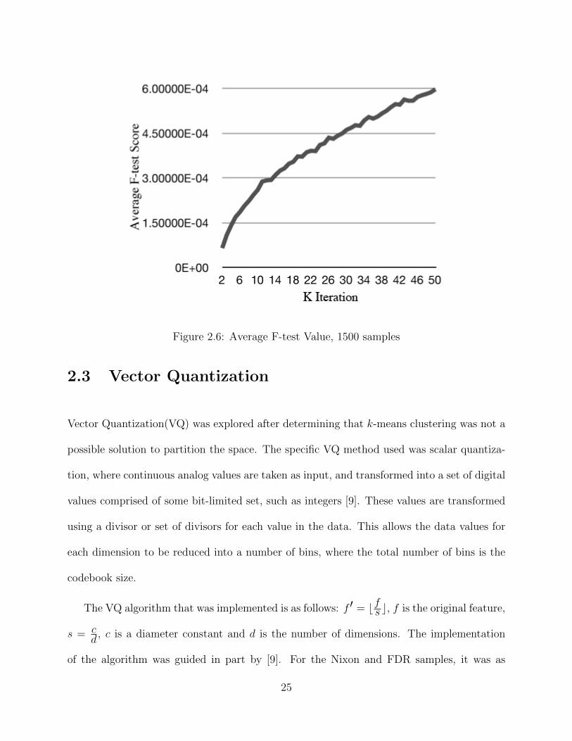
Figure 2.6: Average F-test Value, 1500 samples

2.3 Vector Quantization

Vector Quantization(VQ) was explored after determining that k-means clustering was not a

possible solution to partition the space. The specific VQ method used was scalar quantiza-

tion, where continuous analog values are taken as input, and transformed into a set of digital

values comprised of some bit-limited set, such as integers [9]. These values are transformed

using a divisor or set of divisors for each value in the data. This allows the data values for

each dimension to be reduced into a number of bins, where the total number of bins is the

codebook size.

The VQ algorithm that was implemented is as follows: f ′ = bfs c, f is the original feature,

s = cd

, c is a diameter constant and d is the number of dimensions. The implementation

of the algorithm was guided in part by [9]. For the Nixon and FDR samples, it was as

25

Figure 2.7: Average F-test Value, 3000 samples

follows: f ′ = b f.15625c c = 1.25 and d = 8. The diameter constant was determined from

evaluation of the average diameter as k increased in k-means clustering. In most cases during

the clustering attempts 25 ≤ k ≤ 35 when the average cluster diameter was 1.25 and for

k > 35 minimal decreases in cluster diameter occurred. For values of k < 25 large decreases

in cluster diameter were found when allowing k + 1 to be the limit.

2.4 Performance of Clustering and Vector Quantiza-

tion

The computational complexity of the VQ implementation compared to the k-means is as

follows. When k and the dimension d are restrained, the computational complexity of k-

means is fixed to O(ndk+1logn) where n is the number of vectors. This is case for the

26

different algorithms that were used to measure the validity of k-means, with 2 ≤ k ≤ 100

for most cases (2 ≤ k ≤ 200 for some f-test cases) and d fixed at 8. However, during

convergence there is the possibility that k-means will run forever. This happens if a member

is equidistant from two centroids and is continually assigned from one centroid to the other.

It is also uncommon for k-means to run for exponential time for convergence; it normally

has a polynomial running time[2]. During research the running time was not observed to

be exponential and the assignment algorithm was modified to ensure that equidistant points

did not cause an infinite running time.

The complexity of the VQ algorithm is much less compared to k-means, O(n) where

n is the number of feature vectors. An additional step that was investigated to reduce

the codebook size by taking the standard deviation of the individual dimensions and then

trimming the data to reduce the outliers. This is accomplished by taking data that is larger

than the 3rd deviation and assigning these data to the same value as the boundary 3rd

deviation. This additional computation does not alter the O(n) running time significantly,

keeping the running time O(n).

2.5 Results

The scalar quantization formula described previously was implemented and used to determine

the number of bins created from the test data. Utilizing the randomized samples from the

Roosevelt audio the quantized vectors have a large codebook. Each feature and the number

of possible choices is shown in Table 2.1. The quantized value (QV) standard deviation is

also shown.

The number of possible bins for both feature 1 and 7 are quite high which leads to the

27

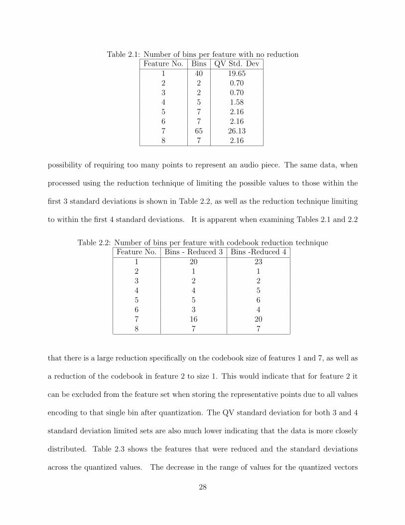
Table 2.1: Number of bins per feature with no reductionFeature No. Bins QV Std. Dev

1 40 19.652 2 0.703 2 0.704 5 1.585 7 2.166 7 2.167 65 26.138 7 2.16

possibility of requiring too many points to represent an audio piece. The same data, when

processed using the reduction technique of limiting the possible values to those within the

first 3 standard deviations is shown in Table 2.2, as well as the reduction technique limiting

to within the first 4 standard deviations. It is apparent when examining Tables 2.1 and 2.2

Table 2.2: Number of bins per feature with codebook reduction techniqueFeature No. Bins - Reduced 3 Bins -Reduced 4

1 20 232 1 13 2 24 4 55 5 66 3 47 16 208 7 7

that there is a large reduction specifically on the codebook size of features 1 and 7, as well as

a reduction of the codebook in feature 2 to size 1. This would indicate that for feature 2 it

can be excluded from the feature set when storing the representative points due to all values

encoding to that single bin after quantization. The QV standard deviation for both 3 and 4

standard deviation limited sets are also much lower indicating that the data is more closely

distributed. Table 2.3 shows the features that were reduced and the standard deviations

across the quantized values. The decrease in the range of values for the quantized vectors

28

Table 2.3: Standard deviation of selected quantized features with codebook reductionFeature No. No reduction Reduced 3 Reduced 4

1 19.65 6.09 7.087 26.13 4.76 6.09

was also coupled with a very negligible increase in the amount of vectors that represent the

data. Table 2.4 shows the original input vector counts and the counts after quantization

that are used to represent the data for both Nixon and Roosevelt. The per file performance

Table 2.4: Number of vectors required to represent the dataData Input vectors Quantized vectors Reduced 3 Reduced 4Nixon 92250 3030 3304 3241

Roosevelt 105000 5481 5716 5723Combined 197250 6932 7365 7355

can be seen in Table 2.5. It is apparent that while using the entire sample set as the data

there are cross-file similarities, but the per-sample set performance does not have the same

reduction level when the input vectors are quantized. Examining the differences in Tables

Table 2.5: Per-sample set average quantizer performanceData avg reduction Avg reduced 3 Avg reduced 4Nixon 50.5% 50.2% 50.4%

Roosevelt 60.2% 60.1% 60.2%

2.4 and 2.5 show that overall there are many vectors that, when quantized, match for the

same speaker. This shows that the scalar quantizer implemented would be a good choice

for using with these features to identify a speaker. It may also be a good indicator for

gender identification due to the high overlap of the 2 data sets when compared against each

other. However, female speaker data is needed to confirm this possibility with the current

prosodic feature set. It may also be possible to enhance the results using a scalar quantizer

per dimension instead of one for the entire vector, similar to how many video codecs use

29

quantization. The approach taken to reduce the codebook size may add additional emphasis

to certain areas in the space due to the values being lumped into the nth standard deviation

bin. A better approach could be to just exclude the data outside the nth standard deviation

to avoid the artificial emphasis of certain areas in the space.

2.6 Conclusion

The ability to partition the space for audio comparison effectively is integral to the whole

of this system. The various methods researched to achieve this have shown that prosodic

features should be treated similarly to cepstral features when partitioning the data. Vector

quantization allows for flexibility in choosing how to partition the space without the ambi-

guity of k-means clustering regarding choosing the correct k. Vector quantization using a

scalar quantizer shows promising results to partition the space and using codebook reduc-

tion techniques reduce the number of possible codes for the quantizer. The results of the

quantization experiments show that using the 8 features selected may prove to be useful

for same-speaker identification and gender identification. It is also possible to remove some

features when using the reduction technique to decrease the space required to store the rep-

resentative points for an audio piece. It was determined that there is a large performance

increase regarding running time using vector quantization over a separate method such as

k-means clustering, with no direct processing penalty for increasing the number of features

being extracted from the audio. Additional data sets and feature sets need to be researched

and tested in order to demonstrate the generality of the system, but the system as proposed

is viable as a framework to do this work.

30

BIBLIOGRAPHY

31

BIBLIOGRAPHY

[1] Charu Aggarwal, Alexander Hinneburg, and Daniel Keim. On the surprising behaviorof distance metrics in high dimensional space. In Database Theory ICDT 2001, volume1973, pages 420–434. Springer Berlin / Heidelberg, 2001.

[2] David Arthur, Bodo Manthey, and Heiko Roglin. k-means has polynomial smoothedcomplexity. Foundations of Computer Science, Annual IEEE Symposium on, 0:405–414,2009.

[3] Benard Bloch and George L. Trager. Outline of linguistic analysis, 1942.

[4] B. Bogert, M. Healy, and J. Tukey. The quefrency alanysis of time series for echoes: Cep-strum, Pseudo-Autocovariance, Cross-Cepstrum and Saphe Cracking. In Proc. Symp.on Time Series Analysis, pages 209–243, 1963.

[5] Douglas R. Caldwell. Unlocking the mysteries of the bounding box. Coordinates: OnlineJournal of the Map and Geography Round Table of the American Library Association,2005.

[6] M.J. Carey, E.S. Parris, H. Lloyd-Thomas, and S. Bennett. Robust prosodic features forspeaker identification. In Fourth International Conference on Spoken Language, 1996.

[7] Charles Darwin. The Descent of Man, volume 2. American Home Library, 1902.

[8] W. Endres, W. Bambach, and G. Flosser. Voice spectrograms as a function of age,voice disguise, and voice imitation. The Journal of the Acoustical Society of America,49(6B):1842–1848, 1971.

[9] Allen Gersho and Robert M. Gray. Vector Quantization and Signal Compression. KluwerAcademic Publishers, 1992.

32

[10] Simon Gunter and Horst Bunke. Validation indices for graph clustering. Pattern Recog-nition Letters, 24(8):1107–1113, 2003.

[11] Margaret Hedstrom, 2003. Technical report, Wave of the Future: NSF Post DigitalLibraries Futures Workshop.

[12] A.K. Jain, M.N. Murty, and P.K. Flynn. Data clustering: A review. ACM ComputingSurveys, 31(3), 1999.

[13] Tomi Kinnunen, Ismo Karkkainen, and Pasi Franti. Is speech data clustered? - statis-tical analysis of cepstral features. In Eurospeech 2001, pages 2627–2630, 2001.

[14] Tomi Kinnunen, Teemu Kilpelainen, and Pasi Franti. Comparison of clustering algo-rithms in speaker identification, 2000.

[15] Chul Min Lee and Shrikanth S. Narayanan. Toward detecting emotions in spoken di-alogs. IEEE Transactions on Speech and Audio Processing, 13(2):293–303, 2005.

[16] John A. Markowitz. Voice biometrics. Communications of the ACM, 43, 2000.

[17] MATRIX. American voices gallery - spoken american culture and history,2009. MATRIX: The center for Humane Arts, Letters, and Social Scienceshttp://www.matrix.msu.edu/ amvoice.

[18] Library of Congress. Fascinating facts - about the library, November 2008.http://www.loc.gov/about/facts.html.

[19] Miller Center of Public Affairs, 2009. http://millercenter.org/scripps/archive/ speeches.

[20] Alan V. Oppenheim and Ronald W. Schafer. From frequency to quefrency: A historyof the cepstrum. IEEE Signal Processing, pages 95–99, 2004.

[21] Gordon E. Peterson and Harold L. Barney. Control methods used in a study of thevowels. The Journal of the Acoustical Society of America, 24(2):175–184, 1952.

[22] Gordon E. Peterson and Ilse Lehiste. Duration of syllable nuclei in english. The Journalof the Acoustical Society of America, 32(6):693–703, 1960.

[23] R. K. Potter and J. C. Steinberg. Toward the specification of speech. The Journal ofthe Acoustical Society of America, 22(6):807–820, 1950.

33

[24] D. Povey, L. Burget, M. Agarwal, P. Akyazi, Kai Feng, A. Ghoshal, O. Glembek,N.K. Goel, M. Karafiat, A. Rastrow, R.C. Rose, P. Schwarz, and S. Thomas. Subspacegaussian mixture models for speech recognition. In 2010 IEEE International Conferenceon Acoustics Speech and Signal Processing, 2010.

[25] Bjorn Schuller, Gerhard Rigoll, and Manfred Lang. Speech emotion recognition com-bining acoustic features and linguistic information in a hybrid support vector machine- belief network architechture. In Proceedings of IEEE International Conference onAcoustics, Speech, and Signal Processing 2004, 2004.

[26] Gideon Schwarz. Estimating the dimension of a model. The Annals of Statistics,6(2):461–464, 1978.

[27] Richard Shenkman. Just How Stupid are We? Facing the Truth About the AmericanVoter. Basic Books, 2008.

[28] E. Shriberg, L. Ferrer, S. Kajarekar, A. Venkataraman, and A. Stolcke. Modelingprosodic feature sequences for speaker recognition. Speech Communication, 46(3-4):455– 472, 2005.

[29] Dagobert Soergel. A framework for digital library research: Broadening the vision.D-Lib Magazine, 8(12), 2002.

[30] George Trager and Benard Bloch. The syllabic phonemes of english. Language, 17(3),1941.

[31] Robert R. Verbrugge, Winifred Strange, Donald P. Shankweiler, and Thomas R. Edman.What information enables a listener to map a talker’s vowel space? The Journal of theAcoustical Society of America, 60(1), 1976.

[32] Avery Li-Chung Wang. An industrial-strength audio search algorithm. In Proceed-ings of the Fourth International Conference on Music Information Retrieval, 2003.www.ismir.net.

[33] Wikipedia, 2009. http://en.wikipedia.org/wiki/Bayesian information criterion.

[34] Tong Zhang. System and method for automatic singer identification. In Proceedings ofIEEE International Conference on Multimedia and Expo, 2003.

34