Computers & Fluids 71 (2013) 306–319

Contents lists available at SciVerse ScienceDirect

Computers & Fluids

journal homepage: www.elsevier .com/locate /compfluid

Partitioned solver for strongly coupled fluid–structure interaction

Charbel Habchi a,b, Serge Russeil a,c,⇑, Daniel Bougeard a,c, Jean-Luc Harion a,c, Thierry Lemenand d,Akram Ghanem d, Dominique Della Valle d,e, Hassan Peerhossaini d,f

a EMDouai, EI, F-59500 Douai, Franceb Energy and Thermo-Fluid Group ETF, School of Engineering, Lebanese International University LIU, PO Box 146404, Mazraa, Beirut, Lebanonc Université Lille Nord de France, F-59000 Lille, Franced Thermofluids, Complex Flows and Energy Research Group, Laboratoire de Thermocinétique de Nantes – CNRS UMR 6607, Nantes University, F-44306 Nantes, Francee ONIRIS, F-44322 Nantes, Francef Univ Paris Diderot, Sorbonne Paris Cité, Institut des Energies de Demain (IED), F-75013 Paris, France

a r t i c l e i n f o a b s t r a c t

Article history:Received 5 December 2011Received in revised form 18 September 2012Accepted 6 November 2012

Keywords:Arbitrary Lagrangian–EulerianAitken’s under-relaxationElastic large deformationSt. Venant–Kirchhoff materialFinite volume methodOpenFOAM

0045-7930/$ - see front matter � 2012 Elsevier Ltd. Ahttp://dx.doi.org/10.1016/j.compfluid.2012.11.004

⇑ Corresponding author at: Ecole des Mines de DouIndustrielle, 941 Rue Charles Bourseul, CS 10838, 595+33 3 27 71 23 88; fax: +33 3 27 71 29 15.

E-mail address: serge.russeil@mines-douai.fr (S. R

In this work a fluid–structure interaction solver is developed in a partitioned approach using blockGauss–Seidel implicit scheme. Finite volume method is used to discretize the fluid flow problem on amoving mesh in an arbitrary Lagrangian–Eulerian formulation and by using an adaptive time step. Thepressure–velocity coupling is performed by using the PIMPLE algorithm, a combination of both SIMPLEand PISO algorithms, which permits the use of larger time steps in a moving mesh. The structural elasticdeformation is analyzed in a Lagrangian formulation using the St. Venant–Kirchhoff constitutive law, fornon-linear large deformations. The solid structure is discretized by the finite volume method in an iter-ative segregated approach. The automatic mesh motion solver is based on Laplace smoothing equationwith variable mesh diffusion. The strong coupling between the different solvers and the equilibriumon the fluid–structure interface are achieved by using an iterative implicit fixed-point algorithm withdynamic Aitken’s relaxation method. The solver, which is called vorflexFoam, is developed using the opensource C++ library OpenFOAM. The solver is validated on two different benchmarks largely used in theopen literature. In the first one the structural deformation is induced by incompressibility. The secondbenchmark consists on a vortex excited elastic flap in a Von Karman vortex street. Finally, a more com-plex case is studied including two elastic flaps immersed in a pulsatile flow. The present solver detectsaccurately the interaction between the complex flow structures generated by the flaps and the effectof the flaps oscillations between each other.

� 2012 Elsevier Ltd. All rights reserved.

1. Introduction

Fluid–structure interaction is a complex multi-physics issuewith contiguous domains consisting generally on viscous fluid flowover elastic solid structures. The elastic structure deforms due tofluid action; mainly pressure and viscous stress. The developmentof robust numerical solvers for fluid–structure interaction prob-lems is a fundamental issue in many engineering fields, such asheat exchangers and chemical reactors, marine cables and petro-leum production risers, aeronautics, vortex induced vibration andnoise, hemodynamics and blood vessel dynamics [1–7].

Two numerical methods can be distinguished as either mono-lithic or partitioned. In the monolithic approach, the completenon-linear system of fluid flow and solid displacement equations

ll rights reserved.

ai, Département Energétique08 Douai Cedex, France. Tel.:

usseil).

are solved simultaneously and are discretized in time and space inthe same manner [7–11]. This fully-coupled or direct approach isknown to be highly robust and stable for very strong fluid–structure interaction including for example phase transformationin material processing, viscoplastic deformation, fracturing due toshocks or detonation [12,13]. However, monolithic methods repre-sent less modularity and require more coding than partitionedapproach in which flow and structural equations are solved by usingindependent suitable algorithms and discretization methods [14–18]. In fact, in the implicit partitioned Dirichlet–Neumannapproach, the flow and structural equations are solved separatelyand the coupling is limited only to the fluid–structure interface.Therefore, an iterative algorithm must be used to handle thecommunication between both flow and structural solvers and to en-force the equilibrium on the fluid–structure interface. This meansthat the fluid flow and the structural deformation are solved succes-sively within an iterating loop until that the difference between theflow and structural solutions, such as the interface displacement, issmaller than a given convergence criterion. The most commonly

C. Habchi et al. / Computers & Fluids 71 (2013) 306–319 307

used coupling methods are the fixed-point method (also calledblock Gauss–Seidel method) [19–21], the interface Newton–Krylovand the quasi-Newton methods [21–25].

Many studies [14–15,18,20,23, 24,26–28] have shown that, theuse of a fixed-point method with dynamic under-relaxation ishighly efficient and easy to implement in partitioned approaches.When the coupling between the fluid flow and the structural defor-mation is strong, due to low solid stiffness or high fluid/structuredensity ratio, the iterations converge slowly and they even may di-verge if the relaxation parameter value is not well chosen. There-fore, the fixed-point iterations can be stabilized and acceleratedby using the Aitken relaxation method where the relaxationparameter is adapted at each iteration using the solution of twoprevious iterations [14,20,29].

Solving fluid–structure interaction problems by implicit fixed-point method can be partitioned into three coupled solvers.

The first one is the fluid flow which solves, for instance, theincompressible Navier–Stokes equations for viscous fluid. Influid–structure interaction problems, the computational domainof the fluid flow is deforming with the fluid–structure interface dis-placement, and thus the Arbitrary Lagrangian–Eulerian (ALE) for-mulation is used to solve the Navier–Stokes equations on adeforming mesh [30–33].

The second solver deals with the structural deformation equa-tions. Generally, the elastic structural deformation can be solvedby using the simple linear formulation by considering the constitu-tive model for a Hookean solid [8,34]. However, for large structuraldisplacement with high strain rates it is more suitable to use thenonlinear formulation where the St. Venant–Kirchhoff constitutivemodel is used for structural analysis [18,35,36]. In contrast to wellestablished finite element methods for computational solidmechanics [6,37,38], Jasak and Weller [34] discretized the linearelastic deformation problem, in Lagrangian formulation, by usingan optimized finite volume method. In this approach, the convec-tive terms are discretized implicitly and the diffusive terms are dis-cretized explicitly, accelerating thus the convergence of the finalsolution. In the present paper, the nonlinear elastic deformationproblem is discretized by using the same method proposed byJasak and Weller [34] and which was recently used by Olivieret al. [36].

The third solver concerns the internal mesh motion which maybe computed using different numerical approaches depending oneither the motion is pure translation, rotation or both translationand rotation as in the present study and in [33,39–44]. In the pres-ent study, the internal mesh motion is solved by using the Laplacesmoothing equation [39,41]. This solver takes the mesh motion atthe fluid–structure interface as boundary conditions and solves theunknown mesh motion equation in the internal fields. Variablemesh diffusivity is used to maintain good mesh quality especiallynear the moving boundary.

In the present study, the open source C++ library OpenFOAM[42,43] is used to implement the different numerical solvers andalgorithms as explained in Sections 2 and 2.4. The originality ofthe solver developed here is that it uses a partitioned finite volumemethod to solve fluid–structure interaction with implicit fixedpoint scheme and dynamic relaxation insuring strong coupling be-tween the solvers. The solid displacement is modeled by the non-linear elastic deformation and Navier–Stokes equations are solvedin ALE approach. As it uses an open source C++ library, this solver isavailable1 for scientific community working on fluid–structureinteraction problems and it can be simply modified to meet the spe-cial need of users. Section 4 is devoted to the validation of the

1 http://www.cfd-online.com/Forums/openfoam/85087-solver-fsi-strongly-coupled-3.html.

numerical solver by comparing the present results with thoseobtained from the literature. In this same section, a more complexcase is studied consisting of two elastic structures fixed on the bot-tom wall in a pulsatile channel flow. Concluding remarks are given inSection 5.

2. Governing equations

2.1. Flow equations

The flow field is governed by the unsteady Navier–Stokes equa-tions for an incompressible viscous flow. The continuity andmomentum equations are respectively given by:

r � uf ¼ 0 ð1Þ

@uf

@tþ uf � ruf ¼ �

rpqfþ tfr2uf ð2Þ

Eqs. (1) and (2) are satisfied in the fluid reference domain Xf,0.For flows without moving mesh, these governing equations canbe discretized by using the Eulerian description where the meshis held fixed [32]. In the Lagrangian formulation, the mesh is fixedto the moving boundary and it moves with it. However, these strat-egies are not valid for computational domains which deform intime as for instance [32]. Therefore, an arbitrary Lagrangian–Eulerian (ALE) formulation [32] is used to handle the flow equa-tions on a deforming mesh, as described in the next section.

2.2. Arbitrary Lagrangian–Eulerian mapping

The arbitrary Lagrangian–Eulerian (ALE) formulation [32] is infact the most commonly used description for fluid–structure inter-action including arbitrary boundary deformation [33,44–46]. Themotion of the interface near the moving structure imposes a con-vective governed flow that is solved by the Lagrangian description.Far away from the structure, the mesh velocity um,f tends to zero sothe equations tend to the Eulerian description.

The fluid domain displacement dm,f is an extension of the soliddisplacement dC0

s from the fluid–structure interface C0 to the inter-nal fluid reference domain Xf,0. Thus, initially, Ddm,f = 0 in Xf,0 anddm;f ¼ dC0

s on C0. The ALE mapping is then defined as in Crosettoet al. [7]:

vðtÞ : Xf ;0 ! Xf ;t

x0#vtðx0Þ ¼ x0 þ dm;fðx0Þð3Þ

The fluid domain velocity can be defined by:

um;f ¼@dm;f

@t

����x0

¼ @vt

@t

����x0

ð4Þ

The ALE formulation of the Navier–Stokes equations that aresatisfied in the updated fluid domain Xf,t is thus [7]:

r � uf ¼ 0 ð5Þ

@uf

@tþ ðuf � um;fÞruf ¼ �

rpqfþ tfr2uf ð6Þ

where (uF � um,f) is the convective term; the Eulerian and Lagrangiandescriptions are obtained respectively by setting um,f = 0 or um,f = uF,with um,f the mesh velocity in the fluid domain.

2.3. Structural equations

The equation of motion for an elastic isothermal solid structurecan be described by the momentum conservation law:

308 C. Habchi et al. / Computers & Fluids 71 (2013) 306–319

qs@us

@t¼ r � rs � qsðrusÞus þ qs f b ð7Þ

where us is the solid velocity us = ods/ ot with ds the displacement ofthe structure, rs is the Cauchy stress tensor and fb is the resultingbody force. Eq. (7) is satisfied in the solid structure domain Xs.

In the present study, the St. Venant–Kirchhoff constitutive law,using an iterative segregated approach in a Lagrangian formula-tion, is implemented to model the elastic structure deformation.This is driven by the fact that this approach is more convenientfor large elastic structure deformation where linear elastic solidmodels fail to describe the structure behavior.

From a Lagrangian point of view, i.e. in terms of the initial con-figuration at t = 0, the momentum balance Eq. (7) is expressed byEq. (8) which is satisfied in the Lagrangian domain Xs,t:

qs@2ds

@t2 ¼ r � ðR � FTÞ þ qs f b ð8Þ

with F the deformation gradient tensor given by:

F ¼ IþrdTs ð9Þ

where I is the identity.The second Piola–Kirchhoff stress tensor R is related to the

Green Lagrangian strain tensor G following [35,36]:X¼ 2lsGþ ks trðGÞI ð10Þ

with G given by:

G ¼ 12ðFT � F� IÞ ð11Þ

here tr is the tensor trace, ks and ls are Lamé constants which arecharacteristics of the elastic material. They are linked to the Youngmodulus E and Poisson’s coefficient ts by:

ks ¼tsE

ð1þ tsÞð1� 2tsÞð12Þ

ls ¼E

2ð1þ tsÞð13Þ

Replacing G, R and F in Eq. (8) by their expressions from Eqs.(9)–(11) gives:

qs@2ds

@t2 ¼ r � lsrds þ lsrdTs þ lsrds � rdT

s þ kstrðrdsÞhn

þ 12

kstrðrds � rdTs Þ�� ðIþrdsÞ

�þ qs f b ð14Þ

This equation is solved in a segregated manner following themethod proposed by Jasak and Weller [34]. Using the Gauss’ theo-rem, the integral form of Eq. (12) over a cell of volume V and sur-face S reads:Z

Vqs@2ds

@t2 dV ¼Z

SdS � ð2ls þ ksÞrds

þZ

Vlsrds þ lsrdT

s þ lsrds � rdTs þ kstrðrdsÞ

hn

þ 12

kstrðrds � rdTs Þ�� ðIþrdsÞ

� 2ls þ ksÞrds þ qs f b

� �dV ð15Þ

This equation is solved before the last step in Fig. 1.Following Jasak and Weller [34], the first term on the right-

hand side, which is a diffusive term, is discretized implicitly. Thesecond term on the right-hand side is treated as a source termand discretized in explicit manner. Jasak and Weller [34] show thatthis discretization method has a significant improvement on theconvergence and stability.

2.4. Coupling and boundary conditions

To establish the equilibrium on fluid–structure interface C,certain conditions must be respected. Primarily the continuity ofdisplacement d, mesh velocity um and equilibrium traction s:

dCs ¼ dC

F ð16Þ

uCs ¼ uC

F ð17Þ

sCs þ sC

F ¼ 0 ð18Þ

where the superscript C denotes the variable at the fluid–structureinterface. Equations (16)–(18) must be satisfied at C.

The traction sF is the sum of viscous forces and pressuresF = pfn + lfruF � n [44,45]. In fact, Eqs. (16) and (17) representthe continuity of the primary quantities at the fluid–structureinterface: the displacement dC

s ¼ dCF and the velocity uC

s ¼ uCF ;

Eq. (18) represents the equilibrium of the dual quantities(action–reaction principle) sC

s þ sCF ¼ 0 including viscous stress

and pressure.The pressure and viscous forces (Eq. (16)) of the fluid flow at the

fluid–structure interface are transferred to the solid as boundaryconditions for the structural solver that computes the displace-ment and stress field in the structure. The displacement velocityis then used as input to solve the mesh motion. The stress fieldof the structural domain is transferred to the flow field as a bound-ary condition on the fluid–structure interface;

rCF ¼ tf devðruF þruT

FÞ ð19Þ

where dev is the deviatoric of a matrix A: dev(A) = A � (1/3)Itr(A).Both the fluid and solid domains are initially at rest. No slip

boundary conditions are imposed on the fluid/structure interfacesor on the other walls. The outlet is set at zero pressure and zeroNeumann for velocity, and a user-defined parabolic velocity profileis set at the flow inlet for the case in question. In fact, these bound-ary conditions depend on the cases studied in Section 4, wheremore complete details on boundary conditions are given for eachcase, especially for the inlet.

3. Numerical procedure

3.1. Spatial and temporal discretization

The open-source C++ toolbox OpenFOAM 1.6-ext [42,45] isused to approximate the fluid flow and structure displacementby using a finite volume approach. The values of all variablesare stored in every control volume center using a collocated var-iable arrangement [45]. A linear scheme with central differencingis used for value interpolation from cell centers to face centers.The surface normal gradients are evaluated at the cell faces andtheir solution algorithm uses an explicit non-orthogonal correc-tion scheme. Laplacian and gradient terms are discretized by sec-ond-order Gaussian integration based on linear interpolation.Gaussian schemes with limited linear differencing interpolationare used for the divergence terms in the flow and structuralsolvers.

In the present study, a non-uniform unstructured conformingquadrilateral mesh is generated using the software Gambit, andis refined at the wall boundaries and fluid–structure interface totake into consideration the high velocity and pressure gradientsin these regions.

Fluid–structure interaction problems with moving solid bound-aries require a third coupled solver for an automatic internal meshmotion. This solver consequently deforms the internal fluiddomain while maintaining the quality and validity of the

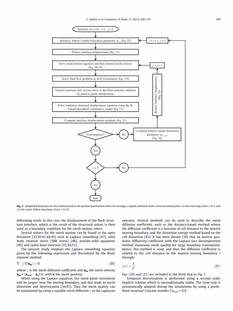
Fig. 1. Simplified flowchart for the method used in the present partitioned solver for strongly coupled nonlinear fluid–structure interaction (i is the time step, from 1 to T, andj is the outer Aitken iterations, from 1 to N).

C. Habchi et al. / Computers & Fluids 71 (2013) 306–319 309

deforming mesh. In this case, the displacement of the fluid–struc-ture interface, which is the result of the structural solver, is thenused as a boundary condition for the mesh motion solver.

Several solvers for the mesh motion can be found in the openliterature [33,39,41,44,45] such as Laplace smoothing [47], solidbody rotation stress (SBR stress) [48], pseudo-solid equations[49] and radial basis function [33,50,51].

The present study employs the Laplace smoothing equationgiven by the following expression and discretized by the finiteelement method:

r � ðcrumÞ ¼ 0 ð20Þ

where c is the mesh diffusion coefficient and um the mesh velocityum = (xt+dt � xt)/dt, with x the mesh position.

When using the Laplace equation, the mesh point movementwill be largest near the moving boundary, and this leads to meshdistortion and deterioration [34,47]. Thus the mesh quality canbe maintained by using a variable mesh diffusion c in the Laplacian

operator. Several methods can be used to describe the meshdiffusion coefficient, such as the distance-based method wherethe diffusion coefficient is a function of cell distance to the nearestmoving boundary, and the distortion-energy method based on thecell distortion [45]. It has been shown [39] that an inverse qua-dratic diffusivity coefficient with the Laplace face decompositionmethod maintains mesh quality for large boundary translations.Hence, this method is used, and thus the diffusion coefficient isrelated to the cell distance to the nearest moving boundary ‘

through:

cð‘Þ ¼ 1‘2 ð21Þ

Eqs. (20) and (21) are included in the third step in Fig. 1.Temporal discretization is performed using a second order

implicit scheme which is unconditionally stable. The time step isautomatically adapted during the simulations by using a prede-fined maximal Courant number Comax = 0.4:

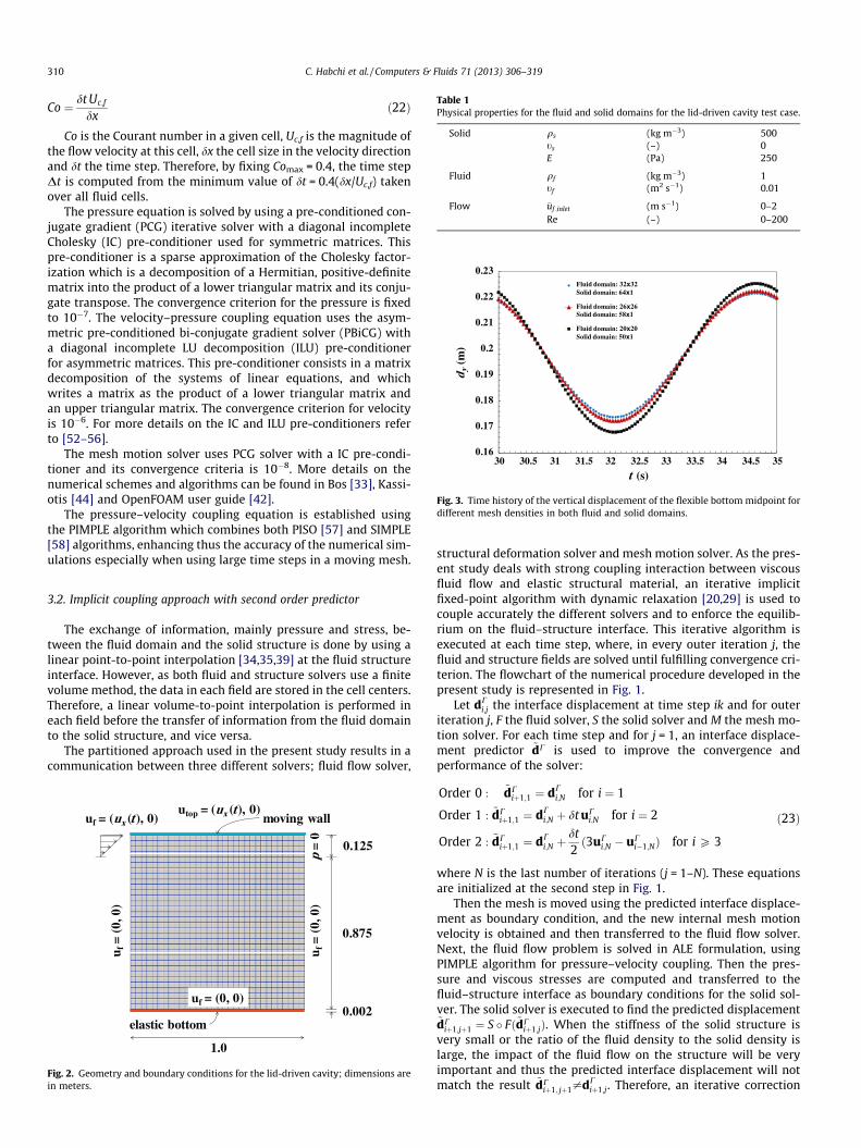
Table 1Physical properties for the fluid and solid domains for the lid-driven cavity test case.

Solid qs (kg m�3) 500ts (–) 0E (Pa) 250

Fluid qf (kg m�3) 1tf (m2 s�1) 0.01

Flow �uf ;inlet (m s�1) 0–2Re (–) 0–200

0.16

0.17

0.18

0.19

0.2

0.21

0.22

0.23

30 30.5 31 31.5 32 32.5 33 33.5 34 34.5 35d y

(m)

t (s)

Fluid domain: 32x32Solid domain: 64x1

Fluid domain: 26x26Solid domain: 58x1

Fluid domain: 20x20Solid domain: 50x1

Fluid domain: 32x32Solid domain: 64x1

Fluid domain: 26x26Solid domain: 58x1

Fluid domain: 20x20Solid domain: 50x1

Fig. 3. Time history of the vertical displacement of the flexible bottom midpoint fordifferent mesh densities in both fluid and solid domains.

310 C. Habchi et al. / Computers & Fluids 71 (2013) 306–319

Co ¼ dt Uc;f

dxð22Þ

Co is the Courant number in a given cell, Uc,f is the magnitude ofthe flow velocity at this cell, dx the cell size in the velocity directionand dt the time step. Therefore, by fixing Comax = 0.4, the time stepDt is computed from the minimum value of dt = 0.4(dx/Uc,f) takenover all fluid cells.

The pressure equation is solved by using a pre-conditioned con-jugate gradient (PCG) iterative solver with a diagonal incompleteCholesky (IC) pre-conditioner used for symmetric matrices. Thispre-conditioner is a sparse approximation of the Cholesky factor-ization which is a decomposition of a Hermitian, positive-definitematrix into the product of a lower triangular matrix and its conju-gate transpose. The convergence criterion for the pressure is fixedto 10�7. The velocity–pressure coupling equation uses the asym-metric pre-conditioned bi-conjugate gradient solver (PBiCG) witha diagonal incomplete LU decomposition (ILU) pre-conditionerfor asymmetric matrices. This pre-conditioner consists in a matrixdecomposition of the systems of linear equations, and whichwrites a matrix as the product of a lower triangular matrix andan upper triangular matrix. The convergence criterion for velocityis 10�6. For more details on the IC and ILU pre-conditioners referto [52–56].

The mesh motion solver uses PCG solver with a IC pre-condi-tioner and its convergence criteria is 10�8. More details on thenumerical schemes and algorithms can be found in Bos [33], Kassi-otis [44] and OpenFOAM user guide [42].

The pressure–velocity coupling equation is established usingthe PIMPLE algorithm which combines both PISO [57] and SIMPLE[58] algorithms, enhancing thus the accuracy of the numerical sim-ulations especially when using large time steps in a moving mesh.

3.2. Implicit coupling approach with second order predictor

The exchange of information, mainly pressure and stress, be-tween the fluid domain and the solid structure is done by using alinear point-to-point interpolation [34,35,39] at the fluid structureinterface. However, as both fluid and structure solvers use a finitevolume method, the data in each field are stored in the cell centers.Therefore, a linear volume-to-point interpolation is performed ineach field before the transfer of information from the fluid domainto the solid structure, and vice versa.

The partitioned approach used in the present study results in acommunication between three different solvers; fluid flow solver,

1.0

0.002

0.875

0.125

uf = (0, 0)

u f=

(0, 0

)

u f=

(0, 0

)

uf = (ux (t ), 0)utop = (ux (t), 0)

elastic bottom

moving wall

p =

0

Fig. 2. Geometry and boundary conditions for the lid-driven cavity; dimensions arein meters.

structural deformation solver and mesh motion solver. As the pres-ent study deals with strong coupling interaction between viscousfluid flow and elastic structural material, an iterative implicitfixed-point algorithm with dynamic relaxation [20,29] is used tocouple accurately the different solvers and to enforce the equilib-rium on the fluid–structure interface. This iterative algorithm isexecuted at each time step, where, in every outer iteration j, thefluid and structure fields are solved until fulfilling convergence cri-terion. The flowchart of the numerical procedure developed in thepresent study is represented in Fig. 1.

Let dCi;j the interface displacement at time step ik and for outer

iteration j, F the fluid solver, S the solid solver and M the mesh mo-tion solver. For each time step and for j = 1, an interface displace-ment predictor ~dC is used to improve the convergence andperformance of the solver:

Order 0 : ~dCiþ1;1 ¼ dC

i;N for i ¼ 1

Order 1 : ~dCiþ1;1 ¼ dC

i;N þ dt uCi;N for i ¼ 2

Order 2 : ~dCiþ1;1 ¼ dC

i;N þdt2ð3uC

i;N � uCi�1;NÞ for i P 3

ð23Þ

where N is the last number of iterations (j = 1–N). These equationsare initialized at the second step in Fig. 1.

Then the mesh is moved using the predicted interface displace-ment as boundary condition, and the new internal mesh motionvelocity is obtained and then transferred to the fluid flow solver.Next, the fluid flow problem is solved in ALE formulation, usingPIMPLE algorithm for pressure–velocity coupling. Then the pres-sure and viscous stresses are computed and transferred to thefluid–structure interface as boundary conditions for the solid sol-ver. The solid solver is executed to find the predicted displacement~dC

iþ1;jþ1 ¼ S � Fð~dCiþ1;jÞ. When the stiffness of the solid structure is

very small or the ratio of the fluid density to the solid density islarge, the impact of the fluid flow on the structure will be veryimportant and thus the predicted interface displacement will notmatch the result ~dC

iþ1; jþ1–dCiþ1;j. Therefore, an iterative correction

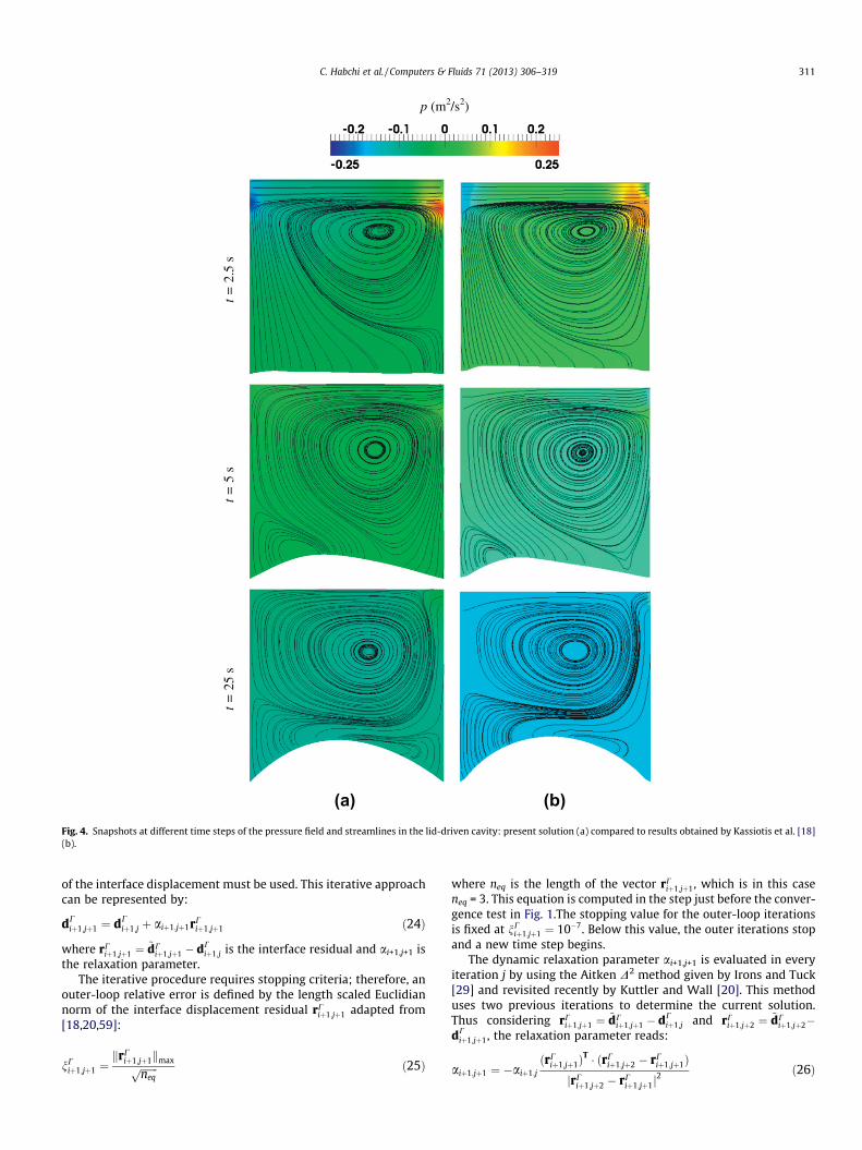
p (m2/s2)

t = 2

.5 s

t =

5 s

t =

25

s

(a) (b)Fig. 4. Snapshots at different time steps of the pressure field and streamlines in the lid-driven cavity: present solution (a) compared to results obtained by Kassiotis et al. [18](b).

C. Habchi et al. / Computers & Fluids 71 (2013) 306–319 311

of the interface displacement must be used. This iterative approachcan be represented by:

dCiþ1;jþ1 ¼ dC

iþ1;j þ aiþ1;jþ1rCiþ1;jþ1 ð24Þ

where rCiþ1;jþ1 ¼ ~dC

iþ1;jþ1 � dCiþ1;j is the interface residual and ai+1,j+1 is

the relaxation parameter.The iterative procedure requires stopping criteria; therefore, an

outer-loop relative error is defined by the length scaled Euclidiannorm of the interface displacement residual rC

iþ1;jþ1 adapted from[18,20,59]:

nCiþ1;jþ1 ¼

krCiþ1;jþ1kmaxffiffiffiffiffiffiffi

neqp ð25Þ

where neq is the length of the vector rCiþ1;jþ1, which is in this case

neq = 3. This equation is computed in the step just before the conver-gence test in Fig. 1.The stopping value for the outer-loop iterationsis fixed at nC

iþ1;jþ1 ¼ 10�7. Below this value, the outer iterations stopand a new time step begins.

The dynamic relaxation parameter ai+1,j+1 is evaluated in everyiteration j by using the Aitken D2 method given by Irons and Tuck[29] and revisited recently by Kuttler and Wall [20]. This methoduses two previous iterations to determine the current solution.Thus considering rC

iþ1;jþ1 ¼ ~dCiþ1;jþ1 � dC

iþ1;j and rCiþ1;jþ2 ¼ ~dC

iþ1;jþ2�dC

iþ1;jþ1, the relaxation parameter reads:

aiþ1;jþ1 ¼ �aiþ1;jðrC

iþ1;jþ1ÞT � ðrC

iþ1;jþ2 � rCiþ1;jþ1Þ

jrCiþ1;jþ2 � rC

iþ1;jþ1j2 ð26Þ

0 10 20 30 40 50 60-0,05

0,00

0,05

0,10

0,15

0,20

0,25

0,30

Gerbeau et al. [14] Kassiotis et al. [18] Vazquez [62] Mok [63] Present results

d y (m

)

t (s)

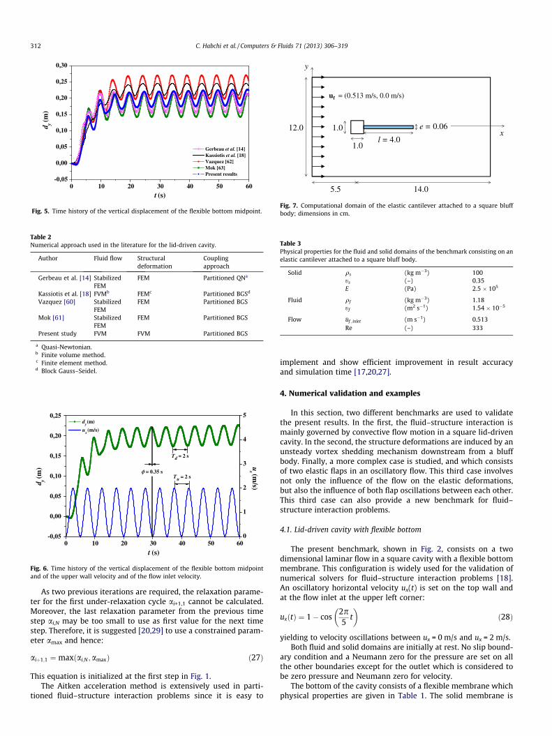
Fig. 5. Time history of the vertical displacement of the flexible bottom midpoint.

Table 2Numerical approach used in the literature for the lid-driven cavity.

Author Fluid flow Structuraldeformation

Couplingapproach

Gerbeau et al. [14] StabilizedFEM

FEM Partitioned QNa

Kassiotis et al. [18] FVMb FEMc Partitioned BGSd

Vazquez [60] StabilizedFEM

FEM Partitioned BGS

Mok [61] StabilizedFEM

FEM Partitioned BGS

Present study FVM FVM Partitioned BGS

a Quasi-Newtonian.b Finite volume method.c Finite element method.d Block Gauss–Seidel.

0 10 20 30 40 50 60-0,05

0,00

0,05

0,10

0,15

0,20

0,25dy (m)

ux (m/s)

Tu = 2 s

t (s)

d y (m

)

Td = 2 s

φ = 0.35 s

0

1

2

3

4

5

ux (m

/s)

Fig. 6. Time history of the vertical displacement of the flexible bottom midpointand of the upper wall velocity and of the flow inlet velocity.

y

xe = 0.06

l = 4.0

14.0

12.0

uf = (0.513 m/s, 0.0 m/s)

1.0

1.0

5.5

Fig. 7. Computational domain of the elastic cantilever attached to a square bluffbody; dimensions in cm.

Table 3Physical properties for the fluid and solid domains of the benchmark consisting on anelastic cantilever attached to a square bluff body.

Solid qs (kg m�3) 100ts (–) 0.35E (Pa) 2.5 � 105

Fluid qf (kg m�3) 1.18tf (m2 s�1) 1.54 � 10�5

Flow �uf ; inlet (m s�1) 0.513Re (–) 333

312 C. Habchi et al. / Computers & Fluids 71 (2013) 306–319

As two previous iterations are required, the relaxation parame-ter for the first under-relaxation cycle ai+1,1 cannot be calculated.Moreover, the last relaxation parameter from the previous timestep ai,N may be too small to use as first value for the next timestep. Therefore, it is suggested [20,29] to use a constrained param-eter amax and hence:

aiþ1;1 ¼maxðai;N ;amaxÞ ð27Þ

This equation is initialized at the first step in Fig. 1.The Aitken acceleration method is extensively used in parti-

tioned fluid–structure interaction problems since it is easy to

implement and show efficient improvement in result accuracyand simulation time [17,20,27].

4. Numerical validation and examples

In this section, two different benchmarks are used to validatethe present results. In the first, the fluid–structure interaction ismainly governed by convective flow motion in a square lid-drivencavity. In the second, the structure deformations are induced by anunsteady vortex shedding mechanism downstream from a bluffbody. Finally, a more complex case is studied, and which consistsof two elastic flaps in an oscillatory flow. This third case involvesnot only the influence of the flow on the elastic deformations,but also the influence of both flap oscillations between each other.This third case can also provide a new benchmark for fluid–structure interaction problems.

4.1. Lid-driven cavity with flexible bottom

The present benchmark, shown in Fig. 2, consists on a twodimensional laminar flow in a square cavity with a flexible bottommembrane. This configuration is widely used for the validation ofnumerical solvers for fluid–structure interaction problems [18].An oscillatory horizontal velocity ux(t) is set on the top wall andat the flow inlet at the upper left corner:

uxðtÞ ¼ 1� cos2p5

t�

ð28Þ

yielding to velocity oscillations between ux = 0 m/s and ux = 2 m/s.Both fluid and solid domains are initially at rest. No slip bound-

ary condition and a Neumann zero for the pressure are set on allthe other boundaries except for the outlet which is considered tobe zero pressure and Neumann zero for velocity.

The bottom of the cavity consists of a flexible membrane whichphysical properties are given in Table 1. The solid membrane is

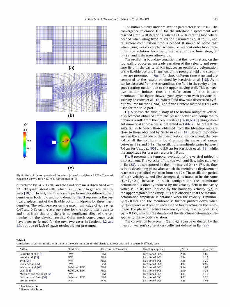
Fig. 8. Mesh of the computational domain at (a) t = 0 s and (b) t = 3.975 s. The meshequiangle skew Q for t = 3.975 is represented in (c).

C. Habchi et al. / Computers & Fluids 71 (2013) 306–319 313

discretized by 64 � 1 cells and the fluid domain is discretized with32 � 32 quadrilateral cells, which is sufficient to get accurate re-sults [18,60]. In fact, mesh tests were performed for different meshdensities in both fluid and solid domains. Fig. 3 represents the ver-tical displacement of the flexible bottom midpoint for three meshdensities. The relative error on the maximum value of dy reaches0.4% and 0.1% on the average value for the second mesh densityand thus from this grid there is no significant effect of the cellnumber on the physical results. Other mesh convergence testshave been performed for the next two cases in Sections 4.2 and4.3, but due to lack of space results are not presented.

Table 4Comparison of current results with those in the open literature for the elastic cantilever a

Author Fluid flow Structural deform

Kassiotis et al. [18] FVM FEMWood et al. [21] FVM FEMYvin [28] FVM FEMOlivier et al. [36] FVM FVMWalhorn et al. [63] Stabilized FEM FEMWall [64] Stabilized FEM FEMMatthies and Steindorf [65] FVM FEMDettmer and Peric [66] Stabilized FEM FEMPresent study FVM FVM

e Block-Newton.f Newton–Raphson.

The initial Aitken’s under relaxation parameter is set to 0.1. Theconvergence tolerance 10�8 for the interface displacement wasreached after 6–10 iterations, whereas 15–18 iterating loop whereneeded when using fixed relaxation parameter equal to 0.1, andthus more computation time is needed. It should be noted thatwhen using weakly coupled scheme, i.e. without outer loop itera-tions, the solution becomes unstable after few time steps, att � 2 s, and it diverges afterwards.

The oscillating boundary conditions, at the flow inlet and on thetop wall, produce an unsteady variation of the velocity and pres-sure field in the cavity which induces an oscillatory deformationof the flexible bottom. Snapshots of the pressure field and stream-lines are presented in Fig. 4 for three different time steps and arecompared to the results obtained by Kassiotis et al. [18]. As itcan be observed from the streamlines, the fluid in the cavity under-goes rotating motion due to the upper moving wall. This convec-tive motion induces thus the deformation of the bottommembrane. This figure shows a good agreement with previous re-sults by Kassiotis et al. [18] where fluid flow was discretized by fi-nite volume method (FVM), and finite element method (FEM) wasused for the solid part.

Fig. 5 shows the time history of the bottom midpoint verticaldisplacement obtained from the present solver and compared toprevious results from the open literature [14,18,60,61] using differ-ent numerical approaches as presented in Table 2. The present re-sults fall in between those obtained from the literature and areclose to those obtained by Gerbeau et al. [14]. Despite the differ-ence in the amplitude of the mean vertical displacement, the per-iod of all the solutions is found almost the same and rangesbetween 4.9 s and 5.1 s. The oscillations amplitude varies between7.4 cm for Vazquez [60] and 3.6 cm for Kassiotis et al. [18], whilethe amplitude for present results is 4.9 cm.

Fig. 6 presents the temporal evolution of the vertical midpointdisplacement. The velocity of the top wall and flow inlet ux, givenin Eq. (28), is also reported. In the time interval 0 < t < 17 s, the flowis in its developing phase after which the membrane displacementreaches its periodical variation from t � 17 s. The oscillation periodof both velocity ux and displacement dy is found to be the same(Td = Tu = 2 s) because in such configuration the membranedeformation is directly induced by the velocity field in the cavitywhich is, in its turn, induced by the boundary velocity ux(t) inthe upper region of the cavity. It is also observed that the maximaldeformation amplitude is obtained when the velocity is minimalux(t) = 0 m/s and the membrane is further pushed down whenux(t) increases as it lead to increase the forces acting on the mem-brane. The phase difference between ux and dy reaches u = 0.35 s,u/T = 0.175, which is the duration of the structural deformation re-sponse to the velocity variation.

The correlation between ux(t) and dy(t) can be evaluated by themean of Pearson’s correlation coefficient defined in Eq. (29):

ttached to square bluff body case.

ation Coupling approach f (s�1) dy,tip (cm)

Partitioned BGS 2.98 1.05Partitioned BGS 2.94 1.15Partitioned BGS 3.16 1.20Partitioned BGS 3.17 0.95Partitioned BGS 3.14 1.02Partitioned BGS 2.99 1.22Partitioned BNe 3.13 1.18Partitioned NRf 3.03 1.25Partitioned BGS 3.25 1.02

fu (m s-1) 2λ (s-1)

t = 3

.980

s

t = 4

.025

s

A

B

t = 4

.075

s

A

B

(a) (b)Fig. 9. Snapshots of (a) the mean flow velocity �uf and (b) k2 criterion for three different time steps.

y

x

2.0 1.0 5.0

0.05

1.0h =

2.0

0.05

A B

Fig. 10. Sketch of the computational domain for two elastic flaps immersed in apulsatile flow; dimensions in meters.

314 C. Habchi et al. / Computers & Fluids 71 (2013) 306–319

! ¼Pn

i¼1½uxðtÞ � �ux�½dyðtÞ � �dy�ðn� 1ÞSux Sdy

ð29Þ

Pearson’s correlation coefficient for the two functions ux and dy

reaches Y = � 0.855 and it is evaluated in the periodic region for17 s < t < 60 s. This negative and relatively high correlation

Table 5Physical properties for the fluid and solid domains of the benchmar

Solid qs (kg m�3)ts (–)E (Pa)

Fluid qf (kg m�3)tf (m2 s�1)

Flow �uf ;max;inlet (m s�1)Re (–)

coefficient value is an evidence of the strong correlation with neg-ative association between the two functions ux and dy. Negativeassociation means that positive values of ux are associated withnegative values of dy.

4.2. Elastic cantilever attached to a square bluff body

While the structural elastic deformation in the previous case isdominated by convective effects, the case shown in Fig. 7 representsa vortex excited elastic flap; a benchmark also widely used for thevalidation of fluid–structure interaction solvers [18,21,28,36,64–67].

This benchmark consists on an elastic cantilever attached to afixed square bluff body immersed in an incompressible flow whichis initially at rest. The top and bottom boundaries are considered

k consisting on two elastic flaps immersed in a pulsatile flow.

TFP1 TFP2

1000 10000.3 0.31 � 106 1 � 105

100 1000.001 0.001

0.25–0.50 0.25–0.50500–1000 500–1000

C. Habchi et al. / Computers & Fluids 71 (2013) 306–319 315

symmetry planes. The flow is uniformly distributed at the inlet (onthe left hand side in Fig. 7) with an imposed streamwise meanvelocity �uinlet ¼ 0:513 m=s. The outlet is considered to be zero pres-sure and Neumann zero for velocity. This velocity corresponds to aReynolds number Re = ux,inletr/tf = 333, based on the bluff bodydimension r = 1 cm, which is higher than the critical Reynolds num-ber beyond which the flow separation from the square corners pro-duces a transient Von Karman vortex street [18,28]. This transientbehavior of the flow induces thus a periodic variation of the pres-sure and viscous stress fields in the near wake of the bluff bodywhich in turns induces the oscillations of the elastic appendix.The physical properties of the fluid and solid domains, representedin Table 3, are chosen so that the vortex shedding frequency is closeto the first Eigen-frequency of the elastic appendix which is 3.03 s�1

[18].The fluid domain contains 15726 quadrilateral cells with mesh

refined on all solid boundaries. The solid structure domain contains2000 quadrilateral cells. The initial mesh of the fluid domain is rep-resented in Fig. 8a showing the grid refined at the wall of thesquare bluff body and near the fluid–structure interface. Fig. 8bshows the deformed mesh for the time step t = 3.975 s where goodmesh quality is always maintained. This quality is represented bythe mean of the equi-angle skew Q in Fig. 8c where it is shown thatits maximal value does not exceed 0.3 emphasizing good meshquality. The solution in the new generated non-orthogonal cellsis corrected in the PIMPLE algorithm. To reach the tolerance onthe interface displacement (Eq. (25)), a maximum number of threeiterations was required. The initial value of the Aitken’s underrelaxation parameter is fixed at 0.3 which rapidly increases to 0.9.

The oscillations frequency and the maximal displacement of thecantilever tip are represented in Table 4. A good agreement isfound with previous results from the open literature. The mean fre-quency of the cantilever oscillation 3.25 s�1 is very close to the the-oretical Eigen-frequency of the elastic appendix which is 3.03 s�1

as its motion is dominated by the first beam Eigen-frequency.The maximal tip motion obtained here dy = 1.02 cm is close to

(szω

t = 2

.7 s

t =

5.1

s

t = 1

2.7

s

(a) Fig. 11. Snapshots of the vorticity xz for both cases (a

those obtained from the open literature by using different solvers,and which ranges between 0.95 cm and 1.25 cm.

The velocity snapshots represented in Fig. 9a for three differenttime steps show an unsteady behavior of the flow which leads, asconsequence, to unsteady oscillations of the elastic cantilever.These oscillations induce in their turn velocity gradients in theflow, near the cantilever tip, which results in the generation ofnew vortices. These vortices can be highlighted by using the k2 cri-terion introduced by Jeong and Hussain [62].

Fig. 9b represents the snapshots of k2 < 0 where the vortex corecan be observed downstream from the bluff body. It can be ob-served that the Von Karman vortex street generated by the squarebluff body is dispersed towards the upper and lower regions due tothe flapping of the elastic cantilever. Moreover, the flap oscillationsgenerates velocity gradients at its tip, thus causing the develop-ment of transient vortices, denoted A and B, advecting downstreamfrom the flap.

4.3. Two elastic flaps immersed in pulsatile flow

In this section, two elastic flaps immersed in a pulsatile flow areconsidered as shown in Fig. 10. Both elastic flaps have the samephysical properties as given in Table 5. Similar properties were alsoused by Olivier and Dumas [16] and Olivier et al. [36] for the caseof one vertical flap in a uniform channel flow. Two different casesare studied, TFP1 and TFP2, which differs by the Young modulusvalue: in the case TFP2 the Young modulus is 10 times smaller thanin TFP1 (see Table 5).

The aim of this study is to present a more complex case wherethe elastic flaps deformation follow a chaotic behavior indepen-dent of the main flow velocity oscillations at the channel inlet.

No slip boundary conditions are set on the two flaps fluid/struc-ture interfaces and on the channel top and bottom walls. The outletis set at zero pressure and zero Neumann for velocity, and a pulsa-tile parabolic velocity profile is set at the flow inlet following asmooth increase from t = 0 s to t = 1 s:

)1−

(b) ) TFP1 and (b) TFP2 for three different time steps.

y

x

(3.025, 1.256)

(0, 0)

0 5 10 15 20

0.0

0.2

0.4

0.6

0.8

1.0 TFP1 TFP2

|U|

(m s

-1)

t (s)

(a)

-14

-12

-10

-8

-6

-4

-2

0

2

4 TFP1 TFP2

ωz

(s-1

)

(b)

0 5 10 15 20t (s)

Fig. 12. Time history of (a) the velocity magnitude and (b) the vorticity field in thepoint (3.025, 1.256).

0 2 4 6 8 10 12 14 16 18 20

-0.02

0.00

0.02

0.04

-0.02

0.00

0.02

0.04

200

400

600

800

1000

d x(m

)

t (s)

1st flap A

2nd flap B

d x(m

)R

e

Fig. 13. Temporal variation of the Reynolds number and of the horizontaldisplacement of the tip of both flaps A and B for the case TFP1.

316 C. Habchi et al. / Computers & Fluids 71 (2013) 306–319

uf ;inlet ¼�uf ;inlet

2½1� cosðptÞ� for t < 1s ð30Þ

uf ;inlet ¼�uf ;inlet

4½3þ cosð2ptÞ� for t P 1s ð31Þ

where �uf ;inlet ¼ umaxyðh� yÞ for 0 < y < h and with umax = 0.5 m/s.Thus, the resulting Reynolds number Re ¼ �uf ;max;inleth=tf , where�uf ;max;inlet ¼ �uf ;inletðx ¼ 0; y ¼ h=2; tÞ is the inlet velocity at the channelcenter, for t P 1 s oscillates between 500 and 1000 with a periodTRe = 1 s.

It should be noted here that the smooth increase in the flowvelocity is important for better numerical stability at the start ofthe simulations and to avoid having a brutal shock on the struc-ture. This method is commonly used in other fluid–structure inter-action problems [67].

The fluid domain mesh consists of 9480 quadrilateral cells re-fined near the wall and fluid–structure interfaces. Each solid struc-ture mesh is composed of 1000 quadrilateral cells. The initial valueof the Aitken’s relaxation parameter is set to 0.1 and a maximalnumber of 12 iterations were needed to reach the convergence cri-terion for the fluid–structure interface displacement.

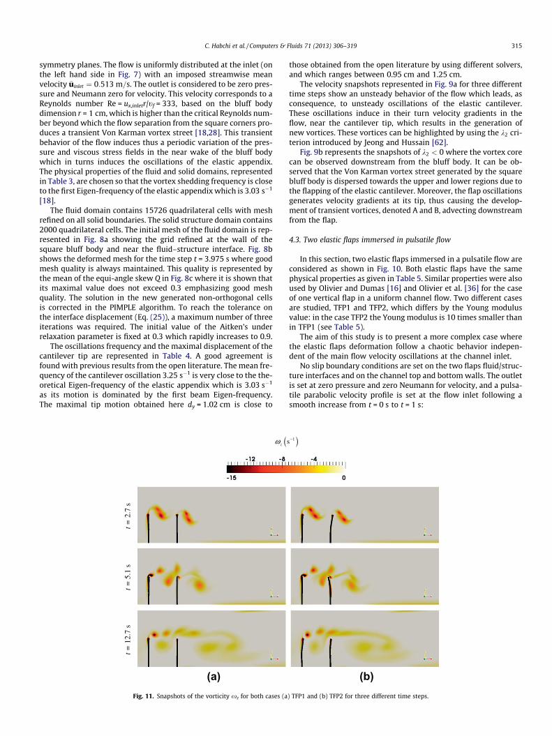
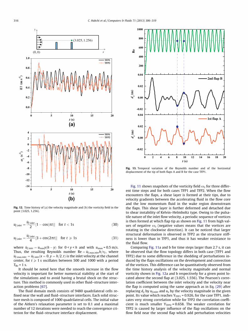
Fig. 11 shows snapshots of the vorticity field xz for three differ-ent time steps and for both cases TFP1 and TFP2. When the flowencounters the flaps, a shear layer is formed at their tips, due tovelocity gradients between the accelerating fluid in the flow coreand the low momentum fluid in the wake region downstreamthe flaps. This shear layer is further deformed and detached dueto shear instability of Kelvin–Helmholtz type. Owing to the pulsa-tile nature of the inlet flow velocity, a periodic sequence of vorticesis then formed at which flap tip as shown on Fig. 11 from high val-ues of negative xz (negative values means that the vortices arerotating in the clockwise direction). It can be noticed that largerstructural deformation is observed in TFP2 as the structure stiff-ness is lower than in TFP1, and thus it has weaker resistance tothe fluid flow.

Comparing Fig. 11a and b for time steps larger than 2.7 s, it canbe observed that the flow topology differs in both case (TFP1 andTFP2) due to some difference in the shedding of perturbations in-duced by the flaps oscillations on the development and convectionof the vortices. This difference can be quantitatively observed fromthe time history analysis of the velocity magnitude and normalvorticity shown in Fig. 12a and b respectively for a given point lo-cated above the second flap at (3.025, 1.556). The Pearson’s corre-lation coefficient between the inlet velocity and the velocity nearthe flap is computed using the same approach as in Eq. (29) afterreplacing dy by uf,inlet and ux by the velocity magnitude in the givenpoint. Its value which reaches YTFP1 = 0.926, for the case TFP1, indi-cates very strong correlation while for TFP2 the correlation coeffi-cient is much smaller YTFP2 = 0.658. The weaker correlation forTFP2 is caused by larger influence of the flap oscillations on theflow field near the second flap which add perturbation velocities

C. Habchi et al. / Computers & Fluids 71 (2013) 306–319 317

to the main flow which is essentially related to the pulsatile inletflow. This can be also observed from the variation of the velocitymagnitude in Fig. 12a, where it represents a quasi-periodic varia-tion for TFP1 with a time period T � 1 s almost the same as thatat the inlet flow velocity. Meanwhile, a quasi-chaotic behaviorfor TFP2 is observed with no characteristic frequency.

The time history of the normal vorticity in Fig. 12b also showsan important difference between both cases TFP1 and TFP2. Largervorticity values are obtained in the vicinity of TFP2 as the higheroscillations induces largest perturbation to the flow and thus in-crease the velocity gradients in the shear layer, which are the prin-cipal cause for the development of the vortex structures asexplained above.

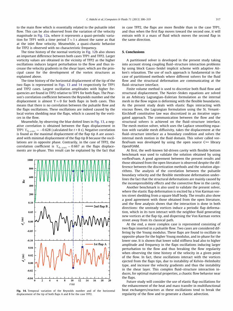
The time history of the horizontal displacement of the tip of thetwo flaps is represented in Figs. 13 and 14 respectively for TFP1and TFP2 cases. Largest oscillation amplitudes with higher fre-quencies are found in TFP2 relative to TFP1 for both flaps. The Pear-son’s correlation coefficient between the Reynolds number and thedisplacement is almost Y � 0 for both flaps in both cases. Thismeans that there is no correlation between the pulsatile flow andthe flaps oscillations. These oscillations are indeed caused by thelocal vortex shedding near the flaps, which is caused by the vorti-ces in the flow.

Meanwhile, by observing the blue dotted lines in Fig. 13, a neg-ative correlation is obtained between the flaps displacement inTFP1 !dA�B;TFP1 ¼ �0:628 (calculated for t > 8 s). Negative correlationis found as the maximal displacement of the flap tip A are associ-ated with minimal displacement of the flap tip B because the oscil-lations are in opposite phase. Contrarily, in the case of TFP2, thecorrelation coefficient is !dA�B;TFP2 ¼ 0:667 as the flaps displace-ments are in-phase. This result can be explained by the fact that

0 2 4 6 8 10 12 14 16 18 20-0.04

-0.02

0.00

0.02

0.04

-0.10

-0.05

0.00

0.05

0.10

200

400

600

800

1000

d x(m

)

t (s)

1st flap A

2nd flap B

d x(m

)R

e

Fig. 14. Temporal variation of the Reynolds number and of the horizontaldisplacement of the tip of both flaps A and B for the case TFP2.

in case TFP2, the flaps are more flexible than in the case TFP1,and thus when the first flap moves toward the second one, it willentrain with it a mass of fluid which moves the second flap inthe same direction.

5. Conclusions

A partitioned solver is developed in the present study takinginto account strong coupling fluid–structure interaction problemsby using block Gauss–Seidel implicit scheme with adaptive Ait-ken’s relaxation. The use of such approach is fundamental in thecase of partitioned methods where different solvers for the fluidflow and the structural deformation are communicating at thefluid–structure interface.

Finite volume method is used to discretize both fluid flow andstructural displacement. The Navier–Stokes equations are solvedin an Arbitrary Lagrangian–Eulerian formulation as the internalmesh in the flow region is deforming with the flexible boundaries.As the present study deals with elastic flaps interacting withviscous flows, the Lagrangian formulation using the St. Venant–Kirchhoff constitutive law was discretized in an iterative segre-gated approach. The communication between the flow and thestructural solvers is achieved on the fluid–structure interface.The mesh motion solver, which uses the Laplace smoothing equa-tion with variable mesh diffusivity, takes the displacement at thefluid–structure interface as a boundary condition and solves theinternal mesh motion in the fluid domain. This solver called vor-flexFoam was developed by using the open source C++ libraryOpenFOAM.

At first, the well-known lid-driven cavity with flexible bottombenchmark was used to validate the solution obtained by usingvorflexFoam. A good agreement between the present results andthose obtained from the open literature is observed despite the dif-ference between the discretization methods and the solution algo-rithms. The analysis of the correlation between the pulsatileboundary velocity and the flexible membrane deformation under-lines the fact that the structural deformations are mainly caused bythe incompressibility effects and the convective flow in the cavity.

Another benchmark is also used to validate the present solver,where the elastic flap deformation is excited by a Von Karman vor-tex street shedding from a square bluff body. The results also showa good agreement with those obtained from the open literature,and the flow analysis shows that the interaction is done in bothdirections: the unsteady vortices induce a periodic flap deforma-tion, which in its turn interact with the neighbor fluid generatingnew vortices at the flap tip, and dispersing the Von Karman vortexstreet away from its classical path.

At the end, a more complex case is represented consisting oftwo flaps inserted in a pulsatile flow. Two cases are considered dif-fering by the Young modulus. These flaps are found to oscillate inopposite-phase for the higher Young modulus, and in-phase for thelower one. It is shown that lower solid stiffness lead also to higheramplitude and frequency in the flaps oscillations inducing largerperturbation to the flow and thus breaking the flow regularitywhen observing the time history of the velocity in a given pointof the flow. In fact, these oscillations interact with the vorticesejected from the flaps tips, due to instability of Kelvin–Helmholtztype, and increase the velocity gradients and thus the instabilityin the shear layer. This complex fluid–structure interaction in-duces, for optimal material properties, a chaotic flow behavior nearthe flaps.

Future study will consider the use of elastic flap oscillations forthe enhancement of the heat and mass transfer in multifunctionalheat exchangers/reactors as these oscillations tend to break theregularity of the flow and to generate a chaotic advection.

318 C. Habchi et al. / Computers & Fluids 71 (2013) 306–319

Acknowledgements

This work is financially supported by the PIE-VORFLEX, CNRS,France. Fruitful discussion with Dr. Sebastien Vintrou and Dr.Sebastien Menanteau from EMDouai-EI are gratefully acknowl-edged. The authors would like also to acknowledge Prof. Guy Du-mas and Mr. Mathieu Olivier from Laval University, Quebec,Canada for enlightening discussions and for providing details ontheir numerical simulations.

References

[1] Newman DJ, Karnidakis GE. A direct numerical simulation study of flow past afreely vibrating cable. J Fluid Mech 1997;344:95–136.

[2] Evangelinos C, Karnidakis GE. Dynamics and flow structures in the turbulentwake of rigid and flexible cylinders subject to vortex-induced vibrations. JFluid Mech 1999;400:91–124.

[3] Parolini N, Quarteroni A. Mathematical models and numerical simulations forthe America’s Cup. Comput Methods Appl Mech Eng 2005;194:1001–26.

[4] Lambert RA, Rangel RH. The role of elastic flap deformation on fluid mixing in amicrochannel. Phys Fluids 2010;22(5):052003.

[5] Habchi C, Lemenand T, Della-Valle D, Peerhossaini H. Turbulence behavior ofartificially generated vorticity. J Turbul 2010;11(36):1–18.

[6] Razzaq M, Damanik H, Hron J, Ouazzi A, Turek S. FEM multigrid techniques forfluid-structure interaction with application to hemodynamics. Appl NumerMath 2012;62(9):1156–70.

[7] Crosetto P, Reymond P, Deparis S, Kontaxakis D, Stergiopulos N, Quarteroni A.Fluid-structure interaction simulation of aortic blood flow. Comput Fluids2011;43(1):46–57.

[8] Greenshields CJ, Weller HG. A unified formulation for continuum mechanicsapplied to fluid–structure interaction in flexible tubes. Int J Numer MethodsEng 2005;64(12):1575–93.

[9] Walhorn E, Kolke A, Hubner B, Dinkler D. Fluid–structure coupling within amonolithic model involving free surface flows. Comput Struct 2005;83(25–26):2100–11.

[10] Heil M, Hazel A, Boyle J. Solvers for large–displacement fluid–structureinteraction problems: segregated versus monolithic approaches. ComputMech 2008;43:91–101.

[11] Badia S, Quaini Q, Quarteroni A. Modular vs. non-modular preconditioners forfluid–structure systems with large added-mass effect. Comput Methods ApplMech Eng 2008;197:4216–32.

[12] Cirak F, Deiterding R, Mauch SP. Large-scale fluid–structure interactionsimulation of viscoplastic and fracturing thin-shells subjected to shocks anddetonations. Comput Struct 2007;85(11–14):1049–65.

[13] Karac A, Blackman B, Cooper V, Kinloch A, Sanchez SR, Teo W, et al. Modellingthe fracture behaviour of adhesively-bonded joints as a function of test rate.Eng Fract Mech 2011;78(6):973–89.

[14] Gerbeau J-F, Vidrascu M, Frey P. Fluid–structure interaction in blood flows ongeometries based on medical imaging. Comput Struct 2005;83(2–3):155–65.

[15] Wall WA, Genkinger S, Ramm E. A strong coupling partitioned approach forfluid–structure interaction with free surfaces. Comput Fluids2007;36(1):169–83.

[16] Olivier M, Dumas G. Non-linear aeroelasticity using an implicit partitionedfinite volume solver. In: Proceedings of the 17th annual conference of the CFDsociety of Canada, Ottawa, Canada; 2009.

[17] Degroote J, Haelterman R, Annerel S, Bruggeman P, Vierendeels J. Performanceof partitioned procedures in fluid-structure interaction. Comput Struct2010;88(7–8):446–57.

[18] Kassiotis C, Ibrahimbegovic A, Niekamp R, Matthies H. Nonlinear fluid-structure interaction problem. Part I: implicit partitioned algorithm,nonlinear stability proof and validation examples. Comput Mech2011;47:305–23.

[19] Tallec PL, Mouro J. Fluid–structure interaction with large structuraldisplacements. Comput Methods Appl Mech Eng 2001;190(24–25):3039–67.

[20] Kuttler U, Wall W. Fixed-point fluid–structure interaction solvers withdynamic relaxation. Comput Mech 2008;43:61–72.

[21] Wood C, Gil A, Hassan O, Bonet J. Partitioned block-Gauss–Seidel couplingfor dynamic fluid–structure interaction. Comput Struct 2010;88(23–24):1367–82.

[22] Michler C, van Brummelen EH, de Borst R. An interface Newton Krylov solverfor fluid–structure interaction. Int J Numer Methods Fluids 2005;47(10–11):1189–95.

[23] Fernández MA, Moubachir M. An exact Block-Newton algorithm for thesolution of implicit time discretized coupled systems involved in fluid–structure interaction problems. In: Bathe KJ, editor. Computational fluid andsolid mechanics 2003. Oxford: Elsevier Science Ltd.; 2003. p. 1337–41.

[24] Fernández MA, Moubachir M. A Newton method using exact Jacobians forsolving fluid–structure coupling. Comput Struct 2005;83:127–42.

[25] Degroote J, Vierendeels J. Multi-solver algorithms for the partitionedsimulation of fluid–structure interaction. Comput Methods Appl Mech Eng2011;200(25–28):2195–210.

[26] Causin P, Gerbeau JF, Nobile F. Added-mass effect in the design of partitionedalgorithms for fluid–structure problems. Comput Methods Appl Mech Eng2005;194:4506–27.

[27] Gallinger T, Bletzinger K. Comparison of algorithms for strongly coupledpartitionned fluid–structure interaction – efficiency versus simplicity. In:Pereira J, Sequeira A, Pereira JM, editors. Proceedings of the V Europeanconference on computational fluid dynamics ECCOMAS CFD, Lisbon, Portugal;2010. p. 1–20.

[28] Yvin C. Partitioned fluid-structure interaction with open-source tools. 12èmeJournées de l’Hydrodynamique, Nantes, France; 2010.

[29] Irons BM, Tuck RC. A version of the Aitken accelerator for computer iteration.Int J Numer Methods Eng 1969;1(3):275–7.

[30] Donea J, Giuliani S, Halleux JP. An arbitrary Lagrangian–Eulerian finite elementmethod for transient dynamic fluid–structure interactions. Comput MethodsAppl Mech Eng 1982;33:689–723.

[31] Souli M, Ouahsine A, Lewin L. ALE formulation for fluid–structure interactionproblems. Comput Methods Appl Mech Eng 2000;190:659–75.

[32] Donea J, Huerta A, Ponthot J-P, Rodriguez-Ferran A. Arbitrary Lagrangian–Eulerian methods. In: Encyclopedia of computational mechanics. John Wiley &Sons, Ltd.; 2004. p. 413–33 [chapter 14].

[33] Bos F. Numerical simulations of flapping foil and wing aerodynamics – meshdeformation using radial basis functions. Ph.D. thesis, the Technical Universityof Delft, Netherlands; 2010.

[34] Jasak H, Weller HG. Application of the finite volume method and unstructuredmeshes to linear elasticity. Int J Numer Methods Eng 2000;48(2):267–87.

[35] Tukovic Z, Jasak H. Updated Lagrangian finite volume solver for largedeformation dynamic response of elastic body. Trans FAMENA2007;31(1):1–16.

[36] Olivier M, Dumas G, Morissette J. A fluid–structure interaction solver for nano-air-vehicle flapping wings. In: Proceedings of the 19th AIAA computationalfluid dynamics conference, San Antonio, USA; 2009. p. 1–15.

[37] Bathe K, Hahn W. On transient analysis of fluid–structure systems. ComputStruct 1979;10(1–2):383–91.

[38] Sathe S, Benney R, Charles R, Doucette E, Miletti J, Senga M, et al. Fluid–structure interaction modeling of complex parachute designs with the space–time finite element techniques. Comput Fluids 2007;36(1):127–35.

[39] Jasak H, Tukovic Z. Automatic mesh motion for the unstructured finite volumemethod. Trans FAMENA 2007;30(2):1–18.

[40] Bos F. Moving and deforming meshes for flapping flight at low reynoldsnumber. In: 3rd OpenFOAM workshop, Milan, Italy; 2008.

[41] Jasak H, Tukovic Z. Dynamic mesh handling in openfoam applied to fluid–structure interation simulations. In: Pereira J, Sequeira A, Pereira JM, editors.Proceedings of the V European conference on computational fluid dynamicsECCOMAS CFD, Lisbon, Portugal; 2010. p. 1–19.

[42] OpenFOAM. The open source CFD toolbox – user guide version 1.7.1; 2010. p.1–204.

[43] Weller HG, Tabor G, Jasak H, Fureby C. A tensorial approach to computationalcontinuum mechanics using object-oriented techniques. Comput Phys1998;12:620–31.

[44] Kassiotis C. Nonlinear fluid-structure interaction: a partitioned approach andits application through component technology. Ph.D. thesis, University ParisEst, France; 2009.

[45] Jasak H, Jemcov A, Tukovic Z. Openfoam: a c++ library for complex physicssimulations. International workshop on coupled methods in numericaldynamics, IUC, Dubrovnik, Croatia; 2007. p. 1–20.

[46] Kassiotis C, Ibrahimbegovic A, Matthies H. Partitioned solution to fluid–structure interaction problem in application to free-surface flows. Eur J Mech –B/Fluids 2010;29(6):510–21.

[47] Lohner R, Yang C. Improved ale mesh velocities for moving bodies. CommunNumer Methods Eng 1996;12(10):599–608.

[48] Dwight RP. Robust mesh deformation using the linear elasticity equations. In:Deconinck H, Dick E, editors. Computational fluid dynamics 2006. Berlin,Heidelberg: Springer; 2009. p. 401–6.

[49] Johnson A, Tezduyar T. Mesh update strategies in parallel finite elementcomputations of flow problems with moving boundaries and interfaces.Comput Methods Appl Mech Eng 1994;119(1–2):73–94.

[50] Krause E. Computational fluid dynamics: its present status and futuredirection. Comput Fluid 1985;13(3):239–69.

[51] Jakobsson S, Amoignon O. Mesh deformation using radial basis functions forgradient-based aerodynamic shape optimization. Comput Fluids2007;36(6):1119–36.

[52] Ferziger J, Peric M. Computational methods for fluid dynamics. 3rded. Berlin: Springer-Verlag; 2002. p. 423.

[53] Behie A, Collins D, Forsyth Jr P. Incomplete factorization methods for three-dimensional non-symmetric problems. Comput Methods Appl Mech Eng1984;42(3):287–99.

[54] Sundholm D. A block preconditioned conjugate gradient method for solvinghigh-order finite element matrix equations. Comput Phys Commun1988;49(3):409–15.

[55] Doi S. On parallelism and convergence of incomplete LU factorizations. ApplNumer Math 1991;7(5):417–36.

[56] Lin CJ, Saigal R. An incomplete Cholesky factorization for dense symmetricpositive definite matrices. BIT Numer Math 2000;40(3):536–58.

[57] Issa RI. Solution of the implicitly discretised fluid flow equations by operator-splitting. J Comput Phys 1986;62(1):40–65.

C. Habchi et al. / Computers & Fluids 71 (2013) 306–319 319

[58] Patankar S, Spalding D. A calculation procedure for heat, mass and momentumtransfer in three-dimensional parabolic flows. Int J Heat Mass Transfer1972;15(10):1787–806.

[59] Deparis S. Numerical analysis of axisymmetric flows and methods for fluidstructure interaction arising in blood flow simulation. Ph.D. thesis, EPFL,Lausanne; 2004.

[60] Vazquez J-G-V. Nonlinear analysis of orthotropic membrane and shellstructures including fluid-structure interaction. Ph.D. thesis, Escola TecnicaSuperior d’Enginyers de Camins, Universitat Politecnica de Catalunya,Barcelone, Espagne, 2007.

[61] Mok DP. Partitionierte losungsansatze in der strukturdynamik und der fluid-struktur-interaktion. Ph.D. thesis, Universitat Stuttgart, Holzgartenstr. 16,70174 Stuttgart; 2001.

[62] Jeong FHJ, Hussain F. On the identification of a vortex. J Fluid Mech1995;285:69–84.

[63] Walhorn E, Hubner B, Dinkler D. Space-time finite elements for fluid-structureinteraction. PAMM 2002;1(1):81–2.

[64] Wall W-A. Fluid–struktur interaktion mit stabilisierten finiten elementen.Ph.D. thesis, Institut fur Baustatik und Baudynamik, Universitat Stuttgart,Germany; 1999.

[65] Matthies HG, Steindorf J. Partitioned strong coupling algorithms for fluid–structure interaction. Comput Struct 2003;81(8–11):805–12.

[66] Dettmer W, Peric D. A computational framework for fluid–structureinteraction: finite element formulation and applications. Comput MethodsAppl Mech Eng 2006;195(41–43):5754–79.

[67] Razzaq M, Hron J, Turek S. Numerical simulation of laminar incompressiblefluid–structure interaction for elastic material with point constraints. In:Rannacher R, Sequeira A, editors. Advances in mathematical fluidmechanics. Berlin, Heidelberg: Springer; 2010. p. 451–72.