PARTITION IDENTITIES AND QUIVER REPRESENTATIONS

RICHARD RIMANYI, ANNA WEIGANDT, AND ALEXANDER YONG

ABSTRACT. We present a particular connection between classical partition combinatoricsand the theory of quiver representations. Specifically, we give a bijective proof of an ana-logue of A. L. Cauchy’s Durfee square identity to multipartitions. We then use this resultto give a new proof of M. Reineke’s identity in the case of quivers Q of Dynkin type A. Ouridentity is stated in terms of the lacing diagrams of S. Abeasis–A. Del Fra, which parame-terize orbits of the representation space of Q for a fixed dimension vector.

CONTENTS

1. Introduction 12. Generating series for partitions 63. Proof of Theorem 1.4 94. Proof of Theorem 1.6 20Acknowledgements 32References 33

1. INTRODUCTION

The main goal of this paper is to establish a specific connection between classical parti-tion combinatorics and the theory of quiver representations. Our motivation is to give anelementary proof for a family of identities introduced by M. Reineke [Rei10]. The iden-tities are closely related to cluster algebras (see e.g., work of V. V. Fock–A. B. Goncharov[FG09] and references therein), wall crossing phenomena (see e.g., the paper [DM16] ofB. Davison–S. Meinhardt as well as the references therein), and Donaldson-Thomas in-variants and Cohomological Hall Algebras (see, e.g., the work of M. Kontsevich–Y. Soibel-man [KS11]). This paper is intended to be an initial step towards understanding the richcombinatorics encoded by advanced dilogarithm identities, such as B. Keller’s identities[Kel11]. We give a new explanation for M. Reineke’s identities in type A via generatingseries arguments.

Following the conventions of [Rim13], we define the quantum dilogarithm series

(1) E(z) =∞∑k=0

(−z)kqk2/2

(1− q)(1− q2) . . . (1− qk).

Date: March 12, 2017.

1

In each term of (1), the denominator may be written more compactly using the q-shiftedfactorial,

(q)k = (1− q)(1− q2) · · · (1− qk).

This has an interpretation in terms of partitions; the reciprocal of (q)k is the generatingseries for partitions with at most k parts [And84, Theorem 1.1].

There are many interesting identities among quantum dilogarithms. We highlight thefollowing, which specializes to the pentagon identity of Rogers’ dilogarithm.

Theorem 1.1 ([Sch53] [FV93], [FK94]). Suppose x and y are formal variables so that yx = qxy.Then

(2) E(x)E(y) = E(y)E(−q1/2xy)E(x).

M. Reineke extended (2) to give a family of identities, one for each Dynkin quiver ([Rei10],[Kel11]). The quantum pentagon identity corresponds to the quiver which has two ver-tices connected by a single edge. In the present work, we show that Theorem 1.1 canactually be proven using the combinatorial tool of Durfee rectangles. In fact, we give aproof of M. Reineke’s identity in type A by proving related identities using iterated Dur-fee rectangles on multipartitions. To state these identities, we first give some necessarybackground on quivers.

A quiver, Q = (Q0,Q1) is a directed graph with vertex set Q0 and arrows Q1. Through-out, we will assume Q has finitely many vertices and identify Q0 with [n] = {1, 2, . . . , n}.For a ∈ Q1, let h(a) be the head of the arrow and t(a) its tail. The Euler form

χQ : Zn × Zn → Z

is defined by

(3) χQ(d1,d2) =∑i∈Q0

d1(i)d2(i)−∑a∈Q1

d1(t(a))d2(h(a)).

DefineλQ(d1,d2) = χQ(d2,d1)− χQ(d1,d2).

Write N for the set of nonnegative integers. Following [Rim13], the quantum algebra AQis generated over Q(q1/2) by

{zd : d ∈ Nn}with multiplication given by

zd1zd2 = −q1/2λQ(d1,d2)zd1+d2 .

Reineke’s identities are among quantum dilogarithms evaluated on elements of AQ. Tostate them, we require some background regarding quiver representations. We brieflyrecall the relevant facts here. For a self contained introduction to quiver representations,see [Bri08]. Throughout, we take C to be our ground field. A representation V of Q is anassignment of a vector space Vi to each i ∈ Q0 and a linear transformation

Va : Vt(a) → Vh(a)

for each arrow a ∈ Q1. Each representation V of Q has an associated dimension vector

dV = (dV(1), . . . ,dV(n)) ∈ Nn, where dV(i) = dimVi.

2

A morphism T : V → W is a collection of linear transformations (Ti : Vi → Wi)i∈Q0

such thatTh(a)Va = WaTt(a) for every arrow a ∈ Q1.

If each of the Ti’s are isomorphisms, then V and W are isomorphic representations.A representation is simple if it has no proper sub-representation. A representation is in-

decomposable if it does not admit a nontrivial decomposition as a direct sum of two rep-resentations. A quiver is Dynkin if its underlying undirected graph is a Dynkin diagramof type ADE. The representation theory of Dynkin quivers is particularly well behaved;if Q is Dynkin, it has finitely many isomorphism classes of simple and indecomposablerepresentations. Furthermore, these classes are uniquely determined by their dimensionvectors.

Theorem 1.2 ([Rei10]). If Q is Dynkin, there exists an ordering on the dimension vectors for thesimple representations α1, . . . , αn and the indecomposable representations β1, . . . , βN so that

(4) E(zα1) · · ·E(zαn) = E(zβ1) · · ·E(zβN).

Proving Theorem 1.2 is equivalent to showing that for every d ∈ Nn the coefficient ofzd is equal on both sides of the expression (4). This calculation of these coefficients iscarried out in [Rim13]. Here, the identity is restated in terms of the geometry of quiverrepresentations.

Let Mat(m,n) be the space of m× n matrices. The representation space is

RepQ(d) :=⊕a∈Q1

Mat(d(h(a)),d(t(a)).

A matrix in Mat(m,n) determines a map from Cn to Cm. As such, points of RepQ(d) deter-mine d dimensional representations of Q. Conversely, any d dimensional representationis isomorphic to some V ∈ RepQ(d). Let

GLQ(d) :=∏x∈Q0

GL(d(x)).

GLQ(d) acts on RepQ(d) by base change. Write OQ(d) for the set of orbits in RepQ(d).Given γ ∈ OQ(d), let codimC(γ) denote the complex codimension of γ in RepQ(d). Pickany representation V ∈ γ. Then by complete reducibility,

V ∼=N⊕i=1

V⊕mβiβi

,

where Vβiis an indecomposable representation so that dim(Vβi

) = βi. In fact, any V′ ∈ γhas this same irreducible decomposition; the mβi

’s are constant on orbits. So we definemβi

(γ) to be the multiplicity of Vβiin the irreducible decomposition of any V ∈ γ.

Theorem 1.3 ([Rim13]). For each dimension vector d = (d(1),d(2), . . . ,d(n)),

(5)n∏

i=1

1

(q)d(i)=

∑γ∈OQ(d)

qcodimC(γ)N∏i=1

1

(q)mβi(γ)

We now restrict our focus to a special case. Assume Q is a type A quiver, i.e. its under-lying graph is just a path on n vertices. We label the vertices from left to right with the set{1, 2, . . . , n}. A lacing diagram [ADF80] L is a graph so that:

3

(1) the vertices are arranged in n columns labeled 1, 2, . . . , n (left to right) and(2) the edges between adjacent columns form a partial matching.

A strand is a connected component of L. A strand is of type [i, j] if it starts in column iand ends in column j. Write

(6) m[i,j](L) = #{strands of type [i, j] in L}.There is an explicit dictionary between representations of Q and lacing diagrams. Eachlacing diagram may be interpreted as a sequence of partial permutation matrices. Thissequence defines a representation VL ∈ RepQ(d). We do not give the details here, as we arenot concerned with the representations themselves, but merely their dimension vectors.See [KMS06] for the equioriented case and [BR07] for quivers of arbitrary orientation.

Let L[i,j] be the lacing diagram that has a single strand of type [i, j]. Define V[i,j] := VL[i,j].

Each V[i,j] is indecomposable. In fact, up to isomorphism, these are the only indecom-posable representations of Q. This is a consequence of Gabriel’s theorem. The simplerepresentations are the special case V[i,i].

The strands in L immediately reveal the irreducible decomposition of VL:

(7) VL ∼=⊕

1≤i≤j≤n

V⊕m[i,j](L)[i,j] .

We associate a dimension vector to L. Write

dim(L) = (dL(1), . . . ,dL(n))

where dL(k) is the number of vertices in column k of L. Equivalently, by counting thenumber of strands which use a vertex of column k, we have

(8) dL(k) =∑

1≤i≤k≤j≤n

m[i,j](L).

Translating from lacing diagrams to representations, we have dim(L) = dim(VL).

Two lacing diagrams are equivalent if they only differ by reordering of vertices withincolumns. For example, the lacing diagrams pictured above are all equivalent. Alterna-tively, we may say

[L] = [L′] if and only if m[i,j](L) = m[i,j](L′) for all 1 ≤ i ≤ j ≤ n.

Therefore, we will write m[i,j]([L]) := m[i,j](L). Using (7), it follows that isomorphismclasses of representations are in bijection with equivalence classes of lacing diagrams:

VL ∼= VL′ if and only if [L] = [L′].

LetCQ(d) = {[L] : dim(L) = d}

denote the set of equivalence classes of d dimensional lacing diagrams. Givenη = [L] ∈ CQ(d), write γη ∈ OQ(d) for the orbit which contains VL. The map η 7→ γηdefines a bijection from CQ(d) → OQ(d).

4

We now associate certain statistics to η. Set parameters

(9) ski (η) = m[i,k−1](η), and

(10) tkj (η) = m[j,k](η) +m[j,k+1](η) + . . .+m[j,n](η).

Let Si denote the ith symmetric group. Fix a sequence of permutations

(11) w = (w(1), . . . , w(n)), where w(i) ∈ Si and w(i)(i) = i.

The partition combinatorics behind Theorem 1.4 below suggests the Durfee statistic:

(12) rw(η) =∑

1≤i<j≤k≤n

skw(k)(i)(η)tkw(k)(j)(η).

With these definitions, we now state our main theorem.

Theorem 1.4 (Quiver Durfee Identity). For d = (d(1), . . . ,d(n)) and w as in (11),

(13)n∏

k=1

1

(q)d(k)=

∑η∈CQ(d)

qrw(η)

n∏k=1

1

(q)tkk(η)

k−1∏i=1

[tki (η) + ski (η)

ski (η)

]q

.

Here [i+ j

j

]q

=(q)i+j

(q)i(q)j

is the q-binomial coefficient, the generating series for partitions with at most i rows and jcolumns [And84, Theorem 3.1]. Indeed, we will show in Lemma 3.1 that each side of (13)has an interpretation as the generating series of a set of multipartitions. By doing somealgebraic cancellations, Theorem 1.4 implies the following:

Corollary 1.5.

(14)n∏

i=1

1

(q)d(i)=

∑η∈CQ(d)

qrw(η)∏

1≤i≤j≤n

1

(q)m[i,j](η)

This is our link to Reineke’s identity. In Definition 4.1, we assign each type A quiver asequence of permutations wQ. We then show this choice satisfies

Theorem 1.6.rwQ(η) = codimC(γη).

For type A, Theorem 1.3 follows as a consequence of Corollary 1.5 and Theorem 1.6.The paper is organized as follows. In Section 2, we recall some background on gen-

erating series. In Section 3, we define sets S and T so that the left hand side of (13) isa generating series for S and the right hand side is a generating series for T . We givean explicit bijection between S and T , thus proving Theorem 1.4. By simple algebraiccancellations, we prove Corollary 1.5. Finally, in Section 4, we prove Theorem 1.6, thuscompleting our proof.

5

2. GENERATING SERIES FOR PARTITIONS

First we recall some background on generating series. Let A be a set equipped with aweight function

wtA : A → N.Suppose

an := |a ∈ A : wt(a) = n| < ∞for each n. Then the generating series for A is

(15) G(A, q) :=∑a∈A

qwtA(a).

Equivalently, by collecting like terms,

(16) G(A, q) =∞∑i=0

aiqi.

Generating series are well behaved under taking products and disjoint unions of sets.Define

wtA×B(a, b) = wtA(a) + wtB(b).

Then

(17) G(A×B, q) = G(A, q)G(B, q).

For disjoint unions, the generating series is additive:

(18) G(A ⊔B, q) = G(A, q) +G(B, q).

Here, we focus on generating series for multipartitions. A partition is a finite sequenceof weakly decreasing, nonnegative integers

λ = (λ1 ≥ λ2 ≥ . . . ≥ λℓ > 0).

The λi are the parts of λ. Define the length of λ to be ℓ(λ) = ℓ, the number of positiveparts of λ. We represent λ visually by its Young diagram, a collection of boxes arrangedin rows so that the number of boxes in row i equals λi. Each partition has an associatedweight

(19) wt(λ) = |λ| =ℓ(λ)∑i=1

λi.

Equivalently, wt(λ) is the total number of boxes in the Young diagram of λ. A multiparti-tion is simply a tuple of partitions λ = (λ(i))i∈I . We weight λ by defining

wt(λ) =∑i∈I

wt(λ(i)).

Let pk = {λ : wt(λ) = k}. Famously due to L. Euler, the generating series for the set of allpartitions is

(20)∞∑k=0

pkqk =

∞∏i=1

1

1− qi.

6

Throughout, we will be interested in subsets of partitions which have constraints placedon the total number of rows or columns in their Young diagram. Let

P(i, j) = {λ : ℓ(λ) ≤ i and λ1 ≤ j}.

Here we allow for i or j to be infinite. When i and j are finite,

(21) G(P(i, j), q) =

[i+ j

i

]q

.

The generating series for P(∞, k), as well as P(k,∞), is obtained by truncating the prod-uct in (20):

(22)1

(q)k=

k∏i=1

1

1− qi.

Write i × j for the rectangular partition with i parts of size j and let R(i, j) = {i × j}.Immediately from (15),

(23) G(R(i, j), q) = qij.

The following identity is due to Euler:

(24)1

(q)∞=

∞∑j=0

qj2

((q)j)2.

We sketch a textbook bijective proof. The Durfee square D(λ) is the largest j × j squarepartition that fits inside λ. Draw D(λ) inside of λ so that it is justified against the topleft corner. By cutting λ along the boundary of D(λ), we may divide λ into three smallerpartitions, as pictured below.

7→

This decomposition defines a bijection:

P(∞,∞)∼−→

∞∪j=0

R(j, j)× P(j,∞)× P(∞, j).

See [And84, pp 27-28] for details and related identities.The present work uses a generalization of the Durfee square. Fix r ∈ Z. The Durfee

rectangle D(λ, r) is the largest i× (i+ r) rectangular partition contained in λ. By conven-tion, we say any 0-width or 0-height rectangle is contained in λ. Equivalently, D(λ, r) isthe rectangle with top left corner positioned at (0, 0) and bottom right corner where theline x+ y = r intersects the (infinite) boundary line of the partition.

Example 2.1. Let λ = (3, 3, 2, 2, 1). Pictured below are the Durfee rectangles D(λ, r) forr = −1, 0, 4.

7

D(λ,−1) D(λ, 0) D(λ, 4)

Notice that D(λ, 4) = 0× 4 rectangle since the line x+ y = 4 intersects the boundary of λat the point (4, 0). �

Decomposing λ using D(λ, r) gives a proof of the following identity of B. Gordon andL. Houten [GH68, pp. 91-92]:

(25)1

(q)∞=

∞∑i=max{0,−r}

qi(r+i)

(q)i(q)r+i

.

The A2 case of Theorem 1.4 can be proved using a truncated version of (25). We sketch theexplicit connection here. Fix r ≤ k. We can split λ ∈ P(∞, k) into three partitions usingD(λ, r). This defines a bijection

P(∞, k)∼−→

k−r∪i=max{0,−r}

R(i, r + i)×P(∞, r + i)× P(i, k − (r + i))

which corresponds to the following identity of generating series:

(26)1

(q)k=

k−r∑i=max{0,−r}

qi(r+i)

(q)r+i

[k − (r + i) + i

i

]q

.

We may rephrase (26) in the language of lacing diagrams. Set n = 2 and fix a dimensionvector d = (k − r, k). Choose a d-dimensional lacing diagram L such that m[1,1](L) = i.Since m[1,1](L)+m[1,2](L) = k−r, necessarily m[1,2](L) = k−r−i. Similarly, m[2,2](L) = r+i.

We reindex the sum in (26) and obtain

(27)1

(q)d(2)=

∑η∈CQ(d)

qm[1,1](η)m[2,2](η)

(q)m[2,2](η)

[m[1,1](η) +m[2,2](η)

m[1,1](η)

]q

.

For any η, we have t11(η) = d(1). Dividing both sides of (27) by (q)d(1) and using theequations (9) and (10) gives

(28)1

(q)d(1)(q)d(2)=

1

(q)d(1)

∑η∈CQ(d)

qs21(η)t

22(η)

(q)t22(η)

[s21(η) + t22(η)

s21(η)

]q

.

We have d(1) = t11(η) for any η ∈ CQ(d). So we obtain

(29)1

(q)d(1)(q)d(2)=

∑η∈CQ(d)

qs21(η)t

22(η)

(q)t11(η)(q)t22(η)

[s21(η) + t22(η)

s21(η)

]q

.

This is the n = 2 case of Theorem 1.4.

8

For n > 2, the proof of Theorem 1.4 uses multiple Durfee rectangles. This technique issimilar to the Durfee dissections of A. Schilling [SW98]. See also the work of C. Boulet onsuccessive Durfee rectangles [Bou10]. We also note the resemblance to the Durfee systemsof P. Bouwknegt [Bou02]. Also see the references to loc. cit. for other work on general-ized Durfee square identities. Our main point of difference is that these identities do notdirectly concern lacing diagrams.

3. PROOF OF THEOREM 1.4

Throughout this section, fix a dimension vector d = (d(1), . . .d(n)) and a sequencepermutations as in (11):

w = (w(1), . . . , w(n)) with w(i) ∈ Si and wi(i) = i.

Define

(30) S = P(∞,d(1))× . . .× P(∞,d(n)).

Let

(31) R(η) = {µ = (µki,j) : µ

ki,j ∈ R(skw(k)(i)(η), t

kw(k)(j)(η)), 1 ≤ i < j ≤ k ≤ n}

which consists of a single element, a tuple of rectangles. For ease of notation, we writeskk(η) = ∞ for each k. Let

(32) P (η) = {ν = (νki ) : ν

ki ∈ P(skw(k)(i)(η), t

kw(k)(i)(η)), 1 ≤ i ≤ k ≤ n}.

Define

(33) T (η) = R(η)× P (η).

Finally, we let

(34) T =∪

η∈CQ(d)

T (η).

Weight λ = (λ(1), . . . , λ(n)) ∈ S by defining

wtS(λ) =n∑

k=1

|λ(k)|.

Assign (µ,ν) ∈ T the weight

wtT (µ,ν) =∑

1≤i<j<k≤n

|µki,j|+

∑1≤i≤k≤n

|νki |.

Lemma 3.1. (1) The generating series for S is

G(S, q) =n∏

k=1

1

(q)d(k).

(2) The generating series for T is

G(T, q) =∑

η∈CQ(d)

qrw(η)

n∏k=1

1

(q)tkk(η)

k−1∏i=1

[tki (η) + ski (η)

ski (η)

]q

.

9

Proof. (1) By (30),S = P(∞,d(1))× . . .× P(∞,d(n)).

Then,

G(S, q) =n∏

k=1

G(P(∞,d(k)), q) (by (17))

=n∏

i=1

1

(q)d(k)(by (22))

(2) First, observe that

G(R(η), q) =∏

1≤i<j≤k≤n

G(R(skw(k)(i)(η), tkw(k)(j)(η)), q) (by (17) and (31))

=∏

1≤i<j≤k≤n

qskw(k)(i)

(η)tkw(k)(j)

(η)(by (23))

= qrw(η) (by (12))

Now,

G(P (η), q) =∏

1≤i≤k≤n

G(P(skw(k)(i)(η), tkw(k)(i)(η)), q) (by (32))

=∏

1≤i≤k≤n

G(P(ski (η), tki (η)), q) (by permuting indices)

=n∏

k=1

G(P(skk(η), tkk(η)), q)

k−1∏i=1

G(P(ski (η), tki (η)), q)

=n∏

k=1

1

(q)tkk(η)

k−1∏i=1

[tki (η) + ski (η)

ski (η)

]q

(by (22) and (21))

Therefore,

G(T, q) =∑

η∈CQ(d)

G(T (η), q) (by (18) and (34))

=∑

η∈CQ(d)

G(R(η)× P (η), q) (by (33))

=∑

η∈CQ(d)

G(R(η), q)G(P (η), q) (by (17))

=∑

η∈CQ(d)

qrw(η)

n∏k=1

1

(q)tkk(η)

k−1∏i=1

[tki (η) + ski (η)

ski (η)

]q

�

We now define the general “cutting” operation we use to map from S to T . Fix twoweakly increasing sequences of nonnegative integers

m = (m0 ≤ m1 ≤ . . . ≤ mkm) and n = (n0 ≤ n1 ≤ . . . ≤ nkn).

10

Given a partition λ, let λ(i,j)(m,n) be the partition formed by restricting the Young dia-gram of λ to rows [mi−1+1,mi] and columns [nj−1+1, nj]. Here, we allow for infinite mkm

and nkn . Immediately from the definition,

(35) λ(i,j)(m,n) ∈ P(mi −mi−1, nj − nj−1).

Furthermore,

(36) λ(i,j)(m,n) ∈ R(mi −mi−1, nj − nj−1)

if and only if the Young diagram of λ has a box in position (mi, nj).The following lemma describes how the size of D(λ, r) varies as r changes.

Lemma 3.2. Fix λ and suppose r′ ≤ r. If D(λ, r) = s× (s+ r) and D(λ, r′) = s′× (s′+ r′) then

(1) s ≤ s′ and(2) s′ + r′ ≤ s+ r.

Proof. (1) Suppose s+r′ < 0. We have 0 ≤ s′+r′, since it is the width of D(λ, r′). Therefore,s ≤ s′. Otherwise, if s+ r′ ≥ 0, the rectangle

s× (s+ r′) ⊆ s× (s+ r) ⊆ λ.

Since D(λ, r′) = s′ × (s′ + r′), we have s ≤ s′.(2) If s = s′ then

s′ + r′ ≤ s′ + r = s+ r.

Then suppose s < s′. Since s+ 1 ≤ s′ and

D(λ, r′) = s′ × (r′ + s′) ⊆ λ,

we have(s+ 1)× (r′ + s′) ⊆ λ.

Since D(λ, r) = s× (s+ r), by definition, (s+ 1)× (s+ 1 + r) ⊆ λ. And so

s′ + r′ ≤ λs+1 < s+ 1 + r,

i.e. s′ + r′ ≤ s+ r. �

Define a map Ψk : T → P(∞,d(k)) by “gluing” the partitions of T with superscript kas indicated in Figure 1. Then let Ψ = Ψ1 × . . .×Ψn.

The proposed inverse Φ : S → T is defined as follows. We will recursively defineparameters

tkj (λ) for 1 ≤ j ≤ k ≤ n

by induction on k. Our initial condition is that t11(λ) = d(1). Assume the sequence

tk−11 (λ), . . . , tk−1

k−1(λ)

has been previously determined and that

tk−1j (λ) ≥ 0 for all 1 ≤ j ≤ k − 1.

Let

(37) δki (λ) = D(λ(k),d(k)−i∑

ℓ=1

tk−1w(k)(ℓ)

(λ)) for i = 0, . . . , k − 1.

11

tkw(k)(k)

tkw(k)(k−1)

tkw(k)(2)

tkw(k)(1)

skw(k)(1)

skw(k)(2)

skw(k)(k−1)

· · ·

...

µk1,k µk

1,k−1 µk1,2

µk2,k µk

2,k−1

µkk−1,k ν

kk−1

νk1

νk2

νkk

FIGURE 1. Description of the map Ψk : T → S.

Note in particular that δk0(λ) = 0× d(k) for all 1 ≤ k ≤ n. Suppose

(38) δki (λ) = aki (λ)× bki (λ) rectangle.

For ease of indexing, write bkk(λ) = 0. Let

(39) tkw(k)(i)(λ) = bki−1(λ)− bki (λ) for i = 1, . . . , k

We also define

(40) skw(k)(i)(λ) = aki (λ)− aki−1(λ) for i = 1, . . . , k − 1

By the hypothesis, tk−1j (λ) ≥ 0 for all 1 ≤ j ≤ k − 1. Therefore,

d(k)−i∑

ℓ=1

tk−1w(k)(ℓ)

(λ)) ≤ d(k)−i−1∑ℓ=1

tk−1w(k)(ℓ)

(λ)) for all i’s .

Then we may apply Lemma 3.2 to the δki ’s, to obtain sequences

(41) ak(λ) = (ak0(λ) ≤ ak1(λ) ≤ · · · ≤ akk−1(λ) ≤ akk(λ))

with akk(λ) = ∞ and

(42) bk(λ) = (bkk(λ) ≤ bkk−1(λ) ≤ · · · ≤ bk1(λ) ≤ bk0(λ)).

By (41) and (42), the ski (λ)’s and tkj (λ)’s are all nonnegative. Continue until k = n.

We then map λ 7→ (µ,ν) where

µki,j = λ(k)(ak(λ),bk(λ))i,k−j+1

12

and

νki = λ(k)(ak(λ),bk(λ))i,k−i+1.

In the proof, we will justify this map is well defined, i.e. (µ,ν) ∈ T . This involvesfinding a class η(λ) ∈ CQ(d) so that (µ,ν) ∈ T (η(λ)). We define our candidate now.

Definition 3.3. Let η(λ) be the equivalence class of a lacing diagram uniquely defined by:

• m[i,j](η(λ)) = sj+1i (λ) for 1 ≤ i ≤ j ≤ n− 1;

• m[i,n](η(λ)) = tni (λ) for i = 1 . . . n.

Since each m[i,j](η(λ)) ≥ 0, we have that η(λ) is well defined.

Example 3.4. Assume w = (1, 12, 123). Fix a dimension vector d = (3, 6, 5) and partitions

λ(1) = (2, 1), λ(2) = (5, 1), and λ(3) = (3, 3, 2, 1, 1).

t11 t21t22

s21

t33 t32 t31

s32

Then δ21(λ) = D(λ(2), 6− 3) = 1× 4 and so t21(λ) = 2, and t22(λ) = 4. From this, we have

δ31(λ) = D(λ(3), 5− 2) = 0× 3 and δ32(λ) = D(λ(3), 5− 2− 4) = 3× 2.

So t31(λ) = 2, t32(λ) = 1, and t33(λ) = 2. This corresponds to η(λ) = [L] where

L =

Alternatively, suppose w = (1, 12, 213). Keeping the same d and λ(i)’s gives

t11 t21t22

s21

t33 t31 t32

s31

s32

As before, δ21(λ) = D(λ(2), 6− 3) = 1× 4. Consequently,

δ31(λ) = D(λ(3), 5− 4) = 2× 3 and δ32(λ) = D(λ(3), 5− 4− 2) = 3× 2.

This yields η(λ) = [L′], where

13

L′ =

�

Immediately from the definitions (9) and (10), we have

(43) tki (η) + ski (η) = tk−1i (η).

for any η ∈ CQ(d). We show the parameters defined in (39) and (40) satisfy the samerecursion.

Lemma 3.5. tkw(k)(i)

(λ) + skw(k)(i)

(λ) = tk−1w(k)(i)

(λ) for 1 ≤ i < k ≤ n.

Proof. By (38) and the definition of a Durfee rectangle,

(44) bki (λ)− aki (λ) = d(k)−i∑

ℓ=1

tk−1w(k)(ℓ)

(λ).

Applying (39) and (40),

tkw(k)(i)(λ) + skw(k)(i)(λ) = bki−1(λ)− bki (λ) + aki (λ)− aki−1(λ)

= (bki−1(λ)− aki−1(λ))− (bki (λ)− aki (λ))

=

(d(k)−

i−1∑ℓ=1

tk−1w(k)(ℓ)

(λ)

)−

(d(k)−

i∑ℓ=1

tk−1w(k)(ℓ)

(λ)

)= tk−1

w(k)(i)(λ). �

The next lemma collects various properties η(λ). In particular, it justifies our choice innotation for ski (λ) and tkj (λ).

Lemma 3.6. (1) ski (η(λ)) = ski (λ)(2) tkj (η(λ)) = tkj (λ)(3) η(λ)) ∈ CQ(d).

Proof. (1) This is immediate from Definition 3.3.(2) By Lemma 3.5,

tki (λ) = tk+1i (λ) + sk+1

i (λ).

Iterating, we obtain

tki (λ) = tk+2i (λ) + sk+2

i (λ) + sk+1i (λ)

= . . .

= tni (λ) +n∑

ℓ=k+1

sℓi(λ)

= tni (η(λ)) +n∑

ℓ=k+1

sℓi(η(λ)) (by Definition 3.3)

14

= m[i,n](η(λ)) +n∑

ℓ=k+1

m[i,ℓ−1](η(λ)) (by (10) and (9))

= tki (η(λ)) (by (10)).

(3) For each k,

d(k) = bk0(λ)− bkk(λ)

=k∑

i=1

bki−1(λ)− bki (λ) (by (39))

=k∑

i=1

tkw(k)(i)(λ)

=k∑

i=1

tki (λ) (permute the terms of the sum)

=k∑

i=1

tki (η(λ)) (by part (2))

=∑

1≤i≤k≤j≤n

m[i,j](η(λ)) (by (10)

By (8), we have η(λ) ∈ CQ(d). �Theorem 3.7. Ψ : T → S is a weight-preserving bijection, i.e., wtT (µ,ν) = wtS(Ψ(µ,ν)).

Proof. Ψ is weight-preserving: That wtT (µ,ν)) = wtS(Ψ(µ,ν)) is clear since Ψ preserves thetotal number of boxes.Ψ is well-defined: If dim(η) = (d(1), . . . ,d(n)) then

d(k) =k∑

i=1

n∑j=k

m[i,j](η) =k∑

i=1

tki (η) for k = 1, . . . , n.

Therefore, Ψk(µ,ν) has parts of size at most d(k) for each k, i.e. Ψk(µ,ν) ∈ P(∞,d(k))for each k. Therefore, Ψ(µ,ν) ∈ S.Φ is well-defined:

By (35),

λ(k)(ak(λ),bk(λ))i,k−j+1 ∈ P(aki (λ)− aki−1(λ), bkj−1(λ)− bkj (λ)).

By (40) and (39),

sw(k)(i)(η(λ)) = aki (λ)− aki−1(λ) and tkw(k)(j)(η(λ)) = bkj−1(λ)− bkj (λ).

Therefore,λ(k)(ak(λ),bk(λ))i,k−j+1 ∈ P(skw(k)(i)(η(λ)), t

kw(k)(j)(η(λ))).

By definition,νki = λ(k)(ak(λ),bk(λ))i,k−i+1

15

and soνki ∈ P (skw(k)(i)(η(λ)), t

kw(k)(i)(η(λ)))

as desired.Similarly, by (35),

µki,j = λ(k)(ak(λ),bk(λ))i,k−j+1

and soµki,j ∈ P(sw(k)(i)(η(λ)), t

kw(k)(j)(η(λ))).

Since δki (λ) ⊂ λ(k), the box (aki (λ), bki (λ)) ∈ λ(k). Likewise, since δkk−j+1(λ) ⊂ λ(k), we have

(akk−j+1(λ), bkk−j+1(λ)) ∈ λ(k).

Therefore, (aki (λ), bkk−j+1(λ)) ∈ λ(k) So, in fact, by (36),

µki,j ∈ R(sw(k)(i)(η(λ)), t

kw(k)(j)(η(λ))).

Therefore, Φ(λ) ∈ T (η(λ)) ⊆ T .Ψ ◦ Φ = Id:

Φ acts by cutting the λ(k)’s into various pieces and Ψ glues these shapes together intotheir original configurations. So for every λ ∈ S, we have Ψ(Φ(λ)) = λ.Φ ◦Ψ = Id:

Fix (µ,ν) ∈ T . Then in particular, (µ,ν) ∈ T (η) for some η ∈ CQ(d). Let λ := Ψ(µ,ν).We must argue η = η(λ). If so, Φ(Ψ(µ,ν)) = (µ,ν).

Since (µ,ν) ∈ T (η), each Ψk(µ,ν) contains a rectangle

(45) ϵkj =

(j∑

i=1

skw(k)(i)(η)

)×

(k∑

i=j+1

tkw(k)(i)(η)

)for all 1 ≤ j < k as in Figure 1.

By definition, dim(η) = d. Then it follows

k∑i=j+1

tkw(k)(i)(η) = d(k)−

(j∑

i=1

tkw(k)(i)(η)

).

As in (43), tki (η) + ski (η) = tk−1i (η). So substituting we have

(46)k∑

i=j+1

tkw(k)(i)(η) = d(k)−j∑

i=1

tk−1wk(i)

(η) +

j∑i=1

skw(k)(i)(η).

Substitution of (46) into (45) yields

ϵkj = s× (s+ d(k)−j∑

i=1

tk−1wk(i)

(η))

contained in λ(k). Here, s =∑j

i=1 ski (η). In particular, by construction, the bottom right

corner of ϵkj intersects the boundary of λ(k) (see Figure 1), i.e. s is the maximum value for

16

which ϵkj ⊆ λ(k). So by the definition of a Durfee rectangle,

ϵkj = D(λ(k),d(k)−j∑

i=1

tk−1wk(i)

(η)).

By (37) and Claim 3.6 part (2),

δkj (λ) = D(λ(k),d(k)−j∑

i=1

tk−1wk(i)

(η(λ)).

We seek to show δkj (λ) = ϵkj for all 1 ≤ j < k ≤ n. Our argument is by induction on k.By definition, t11(η) = d(1) = t11(η(λ)). Then

δ21(λ) = D(λ(2),d(2)− t11(η))

= D(λ(2),d(2)− t11(η(λ))

= ϵ21,

so the Durfee rectangles agree. Assume δk−1j (λ) = ϵk−1

j for all 1 ≤ j < k − 1. Then inparticular, tk−1

i (η) = tk−1i (η(λ)) for all 1 ≤ i ≤ k − 1.

(47)j∑

i=1

tk−1wk(i)

(η) =

j∑i=1

tk−1wk(i)

(η(λ)),

it follows that δkj = ϵkj since both are Durfee rectangles defined by the same parameter.Hence, δkj = ϵkj . Therefore,

ski (η) = ski (η(λ)) for all 1 ≤ i < k ≤ n

andtki (η) = tki (η(λ)) for all 1 ≤ i ≤ k ≤ n.

Hence η = η(λ). �

We now conclude the proof of Theorem 1.4.

Proof. By Theorem 3.7, S and T are in weight preserving bijection. Therefore,

G(S, q) = G(T, q).

Applying Lemma 3.1 gives the result. �

Example 3.8. Let n = 3 and d = (1, 2, 1) and w = (1, 12, 123). Then

rw(η) = (s21(η)t22(η)) + (s31(η)t

32(η) + s31(η)t

33(η) + s32(η)t

33(η))

and

G(P (η), q) =1

(q)t11(η)

1

(q)t22(η)

[t21(η) + s21(η)

s1(η)2

]q

1

(q)t33(η)

[t31(η) + s31(η)

s31(η)

]q

[t32(η) + s32(η)

s32(η)

]q

.

The table below gives the equivalence classes for d = (1, 2, 1) and their correspondingterms on the right hand side of (13).

17

η = [L] (skj (η)) (tkj (η)) G(T (η), q)[ ] 2 1 j/k1 2

2 0 3

3 2 1 j/k1 1

2 0 21 0 0 3

q4(

1(q)1

)(1

(q)2

)(1

(q)1

)= q4

(1−q)3(1−q2)

[ ] 2 1 j/k0 2

1 1 3

3 2 1 j/k1 1

1 1 21 0 0 3

q2(

1(q)1

)(1

(q)1

)(1

(q)1

)= q2

(1−q)3

[ ] 2 1 j/k1 2

1 0 3

3 2 1 j/k1 1

2 0 20 1 0 3

q2(

1(q)1

)(1

(q)2

)([21

]q

)= q2

(1−q)3

[ ] 2 1 j/k0 2

0 1 3

3 2 1 j/k1 1

1 1 20 1 0 3

q(

1(q)1

)(1

(q)1

)= q

(1−q)2

[ ] 2 1 j/k0 2

1 0 3

3 2 1 j/k1 1

1 1 20 0 1 3

(1

(q)1

)(1

(q)1

)= 1

(1−q)2

We then verify,

G(T, q) =q4

(1− q)3(1− q2)+

q2

(1− q)3+

q2

(1− q)3+

q

(1− q)2+

1

(1− q)2

=1

(1− q)3(1− q2)(q4 + 2q2(1− q2) + q(1− q)(1− q2) + (1− q)(1− q2))

=1

(q)1(q)2(q)1= G(S, q).

�

We now give the proof of Corollary 1.5.

Proof. By (43),

(48) tki (η) + ski (η) = tk−1i (η).

Furthermore by (9) and (10),

ski (η) = m[i,k−1](η) and tni (η) = m[i,n](η).

Thus,n∏

k=1

1

(q)tkk(η)

k−1∏i=1

[tki (η) + ski (η)

ski (η)

]q

=n∏

k=1

1

(q)tkk(η)

k−1∏i=1

(q)tki (η)+ski (η)

(q)tki (η)(q)ski (η)

=n∏

k=1

1

(q)tkk(η)

k−1∏i=1

(q)tk−1i (η)

(q)tki (η)(q)ski (η)

18

=

(n∏

k=1

1

(q)tkk(η)

k−1∏i=1

(q)tk−1i (η)

(q)tki (η)

)(n∏

k=1

k−1∏i=1

1

(q)ski (η)

)

=

(n∏

k=1

k∏i=1

1

(q)tki (η)

)(n∏

k=2

k−1∏i=1

(q)tk−1i (η)

)(n∏

k=1

k−1∏i=1

1

(q)ski (η)

)

=

(n∏

k=1

k∏i=1

1

(q)tki (η)

)(n−1∏k=1

k∏i=1

(q)tki (η)

)(n∏

k=1

k−1∏i=1

1

(q)ski (η)

)

=

(n∏

i=1

1

(q)tni (η)

)(n∏

k=1

k−1∏i=1

1

(q)ski (η)

)

=

(n∏

i=1

1

(q)m[i,n](η)

)(n∏

k=1

k−1∏i=1

1

(q)m[i,k−1](η)

)

=∏

1≤i≤j≤n

1

(q)m[i,j](η)

. �

The proof of Theorem 3.7 implies an enriched form of Theorem 1.4. Let

(a; q)k = (1− a)(1− aq)(1− aq2) · · · (1− aqk−1).

For η ∈ CQ(d), let uj(η) be the number of strands that terminate at column j in some(equivalently any) lace diagram L ∈ η. That is,

(49) uj(η) =

j∑i=1

sj+1i (η).

Corollary 3.9 (of Theorem 3.7).

(50)n∏

k=1

1

(qz; q)d(k)=

∑η∈CQ(d)

qrw(η)

n∏k=1

zuk−1(η)1

(qz; q)tkk(η)

k−1∏i=1

[tki (η) + ski (η)

ski (η)

]q

.

Proof. The lefthand side of (50) is the generating series for S with respect to the weightthat uses q to mark the number of boxes and z to mark length of the partitions involved.Now, suppose λ = (λ(1), . . . , λ(n)) ∈ S. Under the indicated decomposition in Figure 1,

ℓ(λ(k)) = ℓ(νkk ) +

k−1∑i=1

skw(k)(i)(η(λ)) = ℓ(νkk ) + uk−1(η(λ)),

where the second equality holds by (49) and reordering terms. The corollary followsimmediately from this and Theorem 3.7 combined. �

Theorem 1.4 is the z = 1 case of Corollary 3.9. By analysis as in Section 2, we obtain asa special case this Durfee rectangle identity:

1

(qz; q)k=

k−r∑i=max{0,−r}

ziqi(r+i)

(qz; q)r+i

[k − (r + i) + i

i

]q

.

From Corollary 3.9 one can deduce an enriched form of Theorem 1.3.

19

4. PROOF OF THEOREM 1.6

Assume Q is a type A quiver. Label its vertices from left to right with the numbers1, 2, . . . , n. Write ai for the arrow whose left endpoint is vertex i. Let I be the set ofintervals in Q, i.e.

I = {[i, j] : i ≤ j and i, j ∈ [n]}.We associate a sequence of permutations to Q as follows:

Definition 4.1. Let w(1)Q = 1 and w

(2)Q = 12. For i ≥ 3 let ι be the natural inclusion from Si−1

to Si and let w(i−1)0 denote the longest permutation in Si−1. Set

w(i)Q =

{ι(w

(i−1)Q ) if ai−2 and ai−1 point in the same direction

ι(w(i−1)Q w

(i−1)0 ) if ai−2 and ai−1 point in opposite directions.

Write wQ := (w(1)Q , . . . , w

(n)Q ). By construction, wQ is of the form (11).

Example 4.2. Let Q be the quiver pictured below.

1 2 3 4 5 6

a1 a2 a3 a4 a5

Then wQ = (1, 12, 123, 3214, 32145, 541236). �

Definition 4.1 is our link between codimC(γη) and the Durfee statistic. The outlineof the proof of Theorem 1.6 is as follows. We start by defining two subsets of I × I,BoxStrands(w) and ConditionStrands(Q). In Proposition 4.3, we show that

rw(η) =∑

(I,J)∈BoxStrands(w)

mI(η)mJ(η).

Proposition 4.10 states

codimC(γη) =∑

(I,J)∈ConditionStrands(Q)

mI(η)mJ(η).

In Proposition 4.13, we show

BoxStrands(wQ) = ConditionStrands(Q).

Combining these propositions completes the proof.

Given a sequence w = (w(1), . . . , w(n)) which satisfies (11), define

(51) BoxStrands(w) = {([w(k)(i), k − 1], [w(k)(j), ℓ]) : 1 ≤ i < j ≤ k ≤ ℓ ≤ n)} ⊆ I × I.

To define ConditionStrands(Q), we consider pairs of intervals (I, J) ∈ I × I of the fol-lowing three types:

(I) I = [w, x− 1] and J = [x, z] with w < x ≤ z

x z

w x− 1

20

(II) I = [w, y] and J = [x, z] with w < x ≤ y < z and the arrows ax−1 and ay point inthe same direction, e.g.,

x z

w y

(III) I = [x, y] and J = [w, z] with w < x ≤ y < z and the arrows ax−1 and ay point indifferent directions, e.g.,

w z

x y

With this, we let

(52) ConditionStrands(Q) = {(I, J) : (I, J) satisfies (I), (II), or (III)}.

The set BoxStrands(w) has an immediate connection to the Durfee statistic rw(η).

Proposition 4.3.

rw(η) =∑

(I,J)∈BoxStrands(w)

mI(η)mJ(η).

Proof. By (12),

rw(η) =∑

1≤i<j≤k≤n

skw(k)(i)(η)tkw(k)(j)(η).

Using (9) and (10), we have:

rw(η) =∑

1≤i<j≤k≤n

m[w(k)(i),k−1](η)

(n∑

ℓ=k

m[w(k)(j),ℓ](η)

)=

∑1≤i<j≤k≤ℓ≤n

m[w(k)(i),k−1](η)m[w(k)(j),ℓ](η)

=∑

(I,J)∈BoxStrands(w)

mI(η)mJ(η). �

We now recall some more facts from the representation theory of quivers. Write Hom(V,W)for the space of morphisms from V to W. Given V and W an extension of V by W is a shortexact sequence of morphisms

0 → W → E → V → 0.

Two extensions are equivalent if the following diagram commutes:

0 W E V 0

0 W E′ V 0

∼

21

Write Ext1(V,W) for the space of extensions of V by W up to equivalence. Hom(V,W) andExt1(V,W) are finite dimensional vector spaces. Recall the Euler form, defined by

χQ(d1,d2) =∑i∈Q0

d1(i)d2(i)−∑a∈Q1

d1(t(a))d2(h(a)).

We often use the abbreviation

χQ(V,W) := χQ(dimV,dimW).

The Euler form satisfies the following:

(53) χQ(V,W) = dimHom(V,W)− dimExt1(V,W),

(see [Bri08, Corollary 1.4.3]).Given I ∈ I, let VI be an irreducible representation indexed by I . Let

(54) Vη =⊕I∈I

V⊕mI(η)I .

Each point in the orbit γη ⊆ RepQ(d) is isomorphic to Vη. The codimension of γη may beexpressed in terms of extensions of Vη. This is Voigt’s lemma (see [Rin80, Lemma 2.3]):

Lemma 4.4 (Voigt).codimC(γη) = dimExt1(Vη,Vη).

Here, we give an alternate expression for codimC(γη) in terms of the Euler form. Define

U = {(I, J) : χQ(VI ,VJ) < 0}.

Lemma 4.5.codimC(γη) =

∑(I,J)∈U

mI(η)mJ(η)(−χQ(VI ,VJ)).

Proof. By [Rei01], Section 2, there exists a total order on I so that

(55) Hom(VI ,VJ) and Ext1(VJ ,VI) = 0 whenever I < J and I = J .

Indecomposables for Dynkin quivers have no nontrivial self extensions, that is,

Ext1(VI ,VI) = 0 for all I ∈ I,[Bri08, Theorem 2.4.3]. So dimExt1(VI ,VJ) = 0 whenever I ≥ J .

WritingVη =

⊕I∈I

V⊕mI(η)I

as a direct sum of indecomposables, we have

Ext1(Vη,Vη) ∼=⊕

(I,J)∈I×I

Ext1(VI ,VJ)⊕mI(η)mJ (η).

ThencodimC(γη) = dimExt1(Vη,Vη) =

∑(I,J)∈I×I

mI(η)mJ(η)dimExt1(VI ,VJ).

Since Ext1(Vη,Vη) vanishes when I ≥ J ,

codimC(γη) =∑

(I,J):I<J

mI(η)mJ(η)dimExt1(VI ,VJ),

22

(see [Rim13]). Combining (53) and (55) gives

codimC(γη) =∑

(I,J):I<J

mI(η)mJ(η)(−χQ(VI ,VJ)).(56)

Using the ordering on I and (53), it follows that

(57) if I < J , then χQ(VI ,VJ) ≤ 0 and χQ(VJ ,VI) ≥ 0.

Since Q is a Dynkin quiver, if I = J , then χQ(VI ,VJ) > 0 [Bri08]. Thus we may reindexthe sum, taking only those (I, J) for which χQ(VI ,VJ) < 0. Therefore,

codimC(γη) =∑

(I,J)∈U

mI(η)mJ(η)(−χQ(VI ,VJ)).

�Lemma 4.6. Fix intervals I and J . If [x, y] ⊆ I, J then

(58)y∑

i=x

dI(i)dJ(i)−y−1∑i=x

dI(t(ai))dJ(h(ai)) = 1

Proof. Since [x, y] ⊆ I, J , dI(i) = dJ(i) = 1 for all i ∈ [x, y]. Therefore,

(59)y∑

i=x

dI(i)dJ(i) = y − x+ 1.

Regardless of the orientation of ai, if i ∈ [x, y − 1] then t(ai), h(ai) ∈ [x, y]. Because[x, y] ⊆ I, J , we have dI(t(ai)) = dJ(h(ai)) = 1. So

(60)y−1∑i=x

dI(t(ai))dJ(h(ai)) = (y − 1)− (x+ 1).

Subtracting (60) from (59) gives (58). �

LetStrandPairs = {(I, J) = ([x1, x2], [y1, y2]) ∈ I × I : x2 ≤ y2}.

From (51) and the definitions (I)-(III), it follows that

ConditionStrands(Q) ⊂ StrandPairs.

Lemma 4.7. Let (I, J) ∈ StrandPairs. Then

(I, J) ∈ ConditionStrands(Q) ⇐⇒ χQ(VI ,VJ) < 0 or χQ(VJ ,VI) < 0.

Moreover, if χQ(VI ,VJ) < 0, then χQ(VI ,VJ) = −1 and likewise χQ(VJ ,VI) < 0 impliesχQ(VJ ,VI) = −1.

Proof. Since we have assumed Q is a type A quiver, we have

(61) χQ(d1,d2) =n∑

i=1

d1(i)d2(i)−n−1∑i=1

d1(t(ai))d2(h(ai)).

Given an interval I , write dI for the dimension vector of VI . By (61), we have

χQ(VI ,VJ) = χQ(dI ,dJ) =n∑

i=1

dI(i)dJ(i)−n−1∑i=1

dI(t(ai))dJ(h(ai)).

23

We analyze this expression repeatedly throughout our argument.(⇒) By direct computation, we will show if (I, J) ∈ ConditionStrands(Q) then

χQ(VI ,VJ) = −1 or χQ(VJ ,VI) = −1,

which is the last assertion of the claim.Case 1: (I, J) = ([w, x− 1], [x, z]) is of type (I).Subcase i: ax−1 points to the right.

χQ(VI ,VJ) =n∑

i=1

dI(i)dJ(i)−n−1∑i=1

dI(t(ai))dJ(h(ai))

= −n−1∑i=1

dI(t(ai))dJ(h(ai)) (since I ∩ J = ∅)

= −dI(t(ax−1))dJ(h(ax−1))

= −dI(x− 1)dJ(x)

= −1

Subcase ii: ax−1 points to the left.Let Qop be the quiver obtained by reversing the direction of all arrows in Q. Then

χQ(dJ ,dI) = χQop(dI ,dJ). Therefore,

χQ(VJ ,VI) = χQ(dJ ,dI) = χopQ (dI ,dJ) = −1

by Subcase 1.i.Case 2: (I, J) = ([w, y], [x, z]) is of type (II).Subcase i: ax−1 and ay point to the right.

χQ(VI ,VJ) =

y∑i=x

dI(i)dJ(i)−y∑

i=x−1

dI(t(ai))dJ(h(ai))

=

(y∑

i=x

dI(i)dJ(i)−y−1∑i=x

dI(t(ai))dJ(h(ai))

)− dI(t(ax−1))dJ(h(ax−1))

− dI(t(ay))dJ(h(ay))

= 1− dI(t(ax−1))dJ(h(ax−1))− dI(t(ay))dJ(h(ay)) (Lemma 4.6)= 1− dI(x− 1)dJ(x)− dI(y)dJ(y + 1)

= −1

Subcase ii: ax−1 and ay point to the left.χQ(VJ ,VI) = −1 by the Qop argument, as in Subcase 1.i.

Case 3: (I, J) = ([x, y], [y, z]) is of type (III).Subcase i: ax−1 points right and ay points left.

χQ(VI ,VJ) =

y∑i=x

dI(i)dJ(i)−y∑

i=x−1

dI(t(ai))dJ(h(ai))

24

=

(y∑

i=x

dI(i)dJ(i)−y−1∑i=x

dI(t(ai))dJ(h(ai))

)− dI(t(ax−1))dJ(h(ax−1))

− dI(t(ay))dJ(h(ay))

= 1− dI(t(ax−1))dJ(h(ax−1))− dI(t(ay))dJ(h(ay)) (Lemma 4.6)= 1− dI(x− 1)dJ(x)− dI(y − 1)dJ(y)

= −1

Subcase ii: ax−1 points left and ay points right.χQ(VJ ,VI) = −1 by the Qop argument, as in Subcase 1.i.Thus we have shown whenever (I, J) ∈ ConditionStrands(Q),

χQ(VI ,VJ) = −1 or χQ(VJ ,VI) = −1.

(⇐) Let (I, J) = ([x1, x2], [y1, y2]) ∈ StrandPairs and first assume χQ(VI ,VJ) < 0.Case 1: I ∩ J = ∅. Then dI(i) = 0 or dJ(i) = 0 for all i ∈ [1, n] and so

χQ(dI ,dJ) = −n−1∑i=1

dI(t(ai))dJ(h(ai)).

Since χQ(dI ,dJ) < 0 there must exist an arrow ai with t(ai) ∈ [x1, x2] and h(ai) ∈ [y1, y2].Then i = x2, ai points to the right, and y1 = x2 + 1. This implies (I, J) is of type (I).Case 2: Assume I ∩ J = ∅. Since we assume x2 ≤ y2

I ∩ J = [x1, x2] ∩ [y1, y2] = [z, x2]

where z ∈ {x1, y1}. Then

χQ(dI ,dJ) =n∑

i=1

dI(i)dJ(i)−n−1∑i=1

dI(t(ai))dJ(h(ai))

=

x2∑i=z

dI(i)dJ(i)−x2∑

i=z−1

dI(t(ai))dJ(h(ai)) (Lemma 4.6)

= 1− dI(t(az−1))dJ(h(az−1))− dI(t(ax2))dJ(h(ax2)).

Since χQ(dI ,dJ) < 0, we must have

dI(t(az−1)) = dJ(h(az−1)) = dI(t(ax2)) = dJ(h(ax2)) = 1.

Therefore,

(62) t(az−1), t(ax2) ∈ I = [x1, x2]

and

(63) h(az−1), h(ax2) ∈ J = [y1, y2].

If an arrow ai points to the right, then h(ai) = i+ 1 and t(ai) = i. If ai points left, h(ai) = iand t(ai) = i + 1. We proceed by analyzing the direction of ax2 and az−1 . First considerax2 . If ax2 points left, then t(ax2) = x2 + 1 and so x2 + 1 ∈ [x1, x2], which is a contradiction.Therefore, we may assume ax2 points right.

Now consider the direction of az−1.

25

If az−1 points to the right, then t(az−1) = z − 1 ∈ [x1, x2] by (62) and so z > x1. Sincez ∈ {x1, y1}, we must have z = y1.

z = y1 y2

x1 x2

Therefore (I, J) is of type (II).If az−1 points left, now we have by (63) h(az−1) = z − 1 ∈ [y1, y2]. Therefore z − 1 > y1

and so z = y1 which implies z = x1. Hence we have:

y1 y2

z = x1 x2

So (I, J) is of type (III).By near identical arguments, χQ(dJ ,dI) < 0 when

(1) az−1 and ax2 both point left, z = y1, and x2 < y2; i.e., (I, J) is of type (II)(2) az−1 points right, ax2 points left, z = x1 and x2 < y2 so (I, J) is of type (III).

�

In particular, we have the following corollary.

Corollary 4.8. If χQ(VI ,VJ) < 0 then χQ(VI ,VJ) = −1

Proof. If (I, J) ∈ StrandPairs, this is immediate by Lemma 4.7. Otherwise, (J, I) ∈StrandParis. Then by Lemma 4.7 (J, I) ∈ ConditionStrands(Q). As such,

χQ(VI ,VJ) = −1.

�

Recall U = {(I, J) : χQ(VI ,VJ) < 0}. We let

U1 = {(I, J) = ([x1, x2], [y1, y2]) : (I, J) ∈ U and x2 ≤ y2}, and

U2 = {(I, J) = ([x1, x2], [y1, y2]) : (I, J) ∈ U and x2 > y2}.Trivially,

(64) U = U1 ⊔ U2

LetU2 = {(J, I) : (I, J) ∈ U2}.

Lemma 4.9. ConditionStrands(Q) = U1 ⊔ U2.

26

Proof. If (I, J) ∈ U2, then (J, I) ∈ U2 ⊂ U and so χQ(VJ ,VI) < 0. Therefore χQ(VI ,VJ) ≥ 0

and hence (I, J) ∈ U . So (I, J) ∈ U1. Therefore, U1 ∩ U2 = ∅.(⊆) If (I, J) ∈ ConditionStrands(Q), by Lemma 4.7, χQ(VI ,VJ) < 0 or χQ(VJ ,VI) < 0.

In the first case, from the definition, (I, J) ∈ U1. In the second case, again by definition,(J, I) ∈ U2, which implies (I, J) ∈ U2.

(⊇) We have U1, U2 ⊆ StrandPairs. Thus by Lemma 4.7, U1, U2 ⊆ ConditionStrands(Q).�

Proposition 4.10.

codimC(γη) =∑

(I,J)∈ConditionStrands(Q)

mI(η)mJ(η).

Proof. If (I, J) ∈ U , then χQ(VI ,VJ) < 0. Applying Corollary 4.8, χQ(VI ,VJ) = −1. Thenby Lemma 4.5,

codimC(γη) =∑

(I,J)∈U

mI(η)mJ(η)(−χQ(VI ,VJ))

=∑

(I,J)∈U

mI(η)mJ(η)

Therefore, applying (64)

codimC(γη) =∑

(I,J)∈U1

mI(η)mJ(η) +∑

(I,J)∈U2

mI(η)mJ(η)

=∑

(I,J)∈U1

mI(η)mJ(η) +∑

(I,J)∈U2

mI(η)mJ(η)

=∑

(I,J)∈ConditionStrands(Q)

mI(η)mJ(η) (Lemma 4.9),

as claimed. �

Our final goal is to show BoxStrands(wQ) = ConditionStrands(Q). We start with alemma.

Lemma 4.11. All elements of BoxStrands(wQ) and ConditionStrands(Q) may be written inthe form:

(65) (I, J) = ([x, k − 1], [y, ℓ]), with x = y, k ≤ ℓ.

Proof. If([w

(k)Q (i), k − 1], [w

(k)Q (j), ℓ]) ∈ Boxstrands(wQ),

thenw

(k)Q (i) = w

(k)Q (j) and k ≤ ℓ.

Hence, by setting x = w(k)Q (i) and y = w

(k)Q (j), we are done.

Now suppose([x1, x2], [y1, y2]) ∈ ConditionStrands(Q).

By definition (I)-(III), x1 = y1 and x2 < y2. So set x = x1, y = y1, k = x2 + 1 and ℓ = y2. �27

With Lemma 4.11 in mind, to prove Boxstrands(wQ) = ConditionStrands(Q), it isenough to show given (I, J) of the form in (65),

(I, J) ∈ BoxStrands(wQ) ⇐⇒ (I, J) ∈ ConditionStrands(Q).

We first handle the special case when I and J are disjoint.

Lemma 4.12. Let (I, J) be as in (65) and suppose I ∩ J = ∅. Then (I, J) ∈ BoxStrands(wQ) ifand only if (I, J) ∈ ConditionStrands(Q).

Proof. If (I, J) ∈ ConditionStrands(Q), then by the disjointness hypothesis it must be oftype (I), i.e.

(I, J) = ([x, k − 1], [k, ℓ]).

Now, since x ≤ k − 1 and w(k)Q ∈ Sk with w

(k)Q (k) = k, there exists i < k such that

w(k)Q (i) = x. So

([x, k − 1], [k, ℓ]) = ([w(k)Q (i), k − 1], [w

(k)Q (k), ℓ]) ∈ BoxStrands(wQ).

Conversely, assume

(I, J) = ([w(k)Q (i), k − 1], [w

(k)Q (j), ℓ]) ∈ BoxStrands(wQ)

and I ∩ J = ∅. Then w(k)Q (j) > k − 1 which means w(k)

Q (j) = k and j = k by the definitionof w(k)

Q . Furthermore, w(k)Q (i) ≤ k − 1 since i < j = k. So

(I, J) = ([w(k)Q (i), k − 1], [k, ℓ])

is of type (I), and hence in ConditionStrands(Q). �

We now show:

Proposition 4.13. BoxStrands(wQ) = ConditionStrands(Q).

Proof. Let (I, J) be as in (65). We seek to show

(I, J) ∈ BoxStrands(wQ) ⇐⇒ (I, J) ∈ ConditionStrands(Q).

We will proceed by induction on k. In the base case k = 2, we must have x = 1 and soy ≥ 2. As such, I ∩ J = ∅ and so we are done by Lemma 4.12. Fix k > 2 and assume theclaim holds for k − 1. That is, given a pair of intervals ([x′, k − 2], [y′, ℓ′]) so that x′, y′ andℓ′ satisfy x′ = y′ and k − 1 ≤ ℓ′ we have(66)([x′, k − 2], [y′, ℓ′]) ∈ BoxStrands(wQ) ⇐⇒ ([x′, k − 2], [y′, ℓ′]) ∈ ConditionStrands(Q).

Now let (I, J) be as in (65), i.e.,

(I, J) = ([x, k − 1], [y, ℓ]), with x = y, k ≤ ℓ.

Again, by Lemma 4.12, if I ∩ J = ∅ we are done, so assume I ∩ J = ∅. Then y < k.Now, since 1 ≤ x, y ≤ k, there exist i and j such that

1 ≤ i, j ≤ k with x = w(k)(i) and y = w(k)(j).

So from (51)

(67) (I, J) = ([w(k)Q (i), k − 1], [w

(k)Q (j), ℓ]) ∈ BoxStrands(wQ) ⇐⇒ i < j.

28

Throughout, when x ≤ k − 2 we write I ′ := [x, k − 2]. We will break the argument intotwo main cases.Case 1: ak−2 and ak−1 point in the same direction.

By definition, w(k)Q = ι(w

(k−1)Q ). Then if x ≤ k − 2, it follows that

(I ′, J) = ([x, k − 2], [y, ℓ])

= ([wk−1Q (i), k − 2], [wk−1

Q (j), ℓ])

and so

(68) (I ′, J) ∈ BoxStrands(wQ) if and only if i < j.

We have four possible subcases, based on the relative values of x and y.Subcase i: x < y = k − 1.

(I, J) is of type (II), and hence (I, J) ∈ ConditionStrands(Q). Furthermore, note that

(I ′, J) = ([x, k − 2], [k − 1, ℓ])

is of type (I), and so in ConditionStrands(Q). The intervals for (I ′, J) and (I, J) look likethis:

x k − 2

k − 1 ℓ

x k − 1

k − 1 ℓ .

By the inductive hypothesis (66), (I ′, J) ∈ BoxStrands(wQ). By (68), i < j. Therefore, by(67), (I, J) ∈ BoxStrands(wQ).

Therefore, (I, J) is in both ConditionStrands(Q) and BoxStrands(wQ).Subcase ii: x < y < k − 1.

(I, J) ∈ BoxStrands(wQ) ⇐⇒ i < j by (67)

⇐⇒ (I ′, J) ∈ BoxStrands(wQ) by (68)

⇐⇒ (I ′, J) ∈ ConditionStrands(Q) by (66)⇐⇒ ax−1 points in the same direction as ak−2

⇐⇒ ax−1 points in the same direction as ak−1

⇐⇒ (I, J) ∈ ConditionStrands(Q).

The following picture depicts (I ′, J) and (I, J) respectively when (I ′, J) and (I, J) are inConditionStrands(Q).

y ℓ

x k − 2

y ℓ

x k − 1

Subcase iii: y < x = k − 1.Pictured below are the intervals I and J .

29

y ℓ

x

Since y < x and this case assumes ak−2 and ak−1 point in the same direction, (I, J) cannotbe of type (III) and is not in ConditionStrands(Q). Since

w(k)Q = ιw

(k−1)Q and w

(k−1)Q (k − 1) = k − 1,

it follows that i = k − 1. Since

y = w(k)Q (j) = w

(k−1)Q (j) < k − 1,

it follows that i > j, and so by (67)

(I, J) ∈ BoxStrands(wQ).

Therefore, (I, J) is in neither ConditionStrands(Q) nor BoxStrands(wQ).Subcase iv: y < x < k − 1.

(I, J) ∈ BoxStrands(wQ) ⇐⇒ i < j by (67)

⇐⇒ (I ′, J) ∈ BoxStrands(wQ) by (68)

⇐⇒ (I ′, J) ∈ ConditionStrands(Q) by (66)⇐⇒ ax−1 points in the opposite direction as ak−2

⇐⇒ ax−1 points in the opposite direction as ak−1

⇐⇒ (I, J) ∈ ConditionStrands(Q).

Below are (I ′J) and (I, J) respectively, in the case (I ′, J), (I, J) ∈ ConditionStrands(Q).

y ℓ

x k − 2

y ℓ

x k − 1

Case 2: ak−2 and ak−1 point in opposite directions.By definition,

w(k)Q = ι(w

(k−1)Q w

(k−1)0 ).

If x ≤ k − 2, and y ≤ k − 1 it follows that

(I ′, J) = ([x, k − 2], [y, ℓ])

= ([w(k−1)Q (k − i), k − 2], [w

(k−1)Q (k − j), ℓ])

and so

(69) (I ′, J) ∈ BoxStrands(wQ) if and only if k − i < k − j if and only if i > j.

Subcase i: x < y = k − 1.

30

x k − 2

k − 1 ℓ

x k − 1

k − 1 ℓ

Since ak−2 and ak−1 point in opposite directions, (I, J) ∈ ConditionStrands(Q). The as-sumption y = k−1 implies (I ′, J) ∈ ConditionStrands(Q). By (66) (I ′, J) ∈ BoxStrands(wQ).Since x, y < k, we have

x = w(k)Q (i) = w

(k−1)Q (k − i) and y = w

(k)Q (j) = w

(k−1)Q (k − j).

Then k − i < k − j, so i > j and (I, J) ∈ BoxStrands(wQ), by (67).Hence (I, J) is neither in ConditionStrands(Q) nor BoxStrands(wQ).

Subcase ii: x < y < k − 1.

(I, J) ∈ BoxStrands(wQ) ⇐⇒ i < j by (67)

⇐⇒ (I ′, J) ∈ BoxStrands(wQ) by (69)

⇐⇒ (I ′, J) ∈ ConditionStrands(Q) by (66)⇐⇒ ay−1 points in the opposite direction as ak−2

⇐⇒ ay−1 points in the same direction as ak−1

⇐⇒ (I, J) ∈ ConditionStrands(Q).

Below, we have (I ′, J) ∈ ConditionStrands(Q) and (I, J) ∈ ConditionStrands(Q).

y ℓ

x k − 2

y ℓ

x k − 1

Subcase iii: y < x = k − 1. Here (I, J) looks like:

y ℓ

x

Since Case 2 assumes ak−2 and ak−1 point in opposite directions, (I, J) is type (II) and soin ConditionStrands(Q). Now,

k − 1 = x = w(k)Q (i) = w

(k−1)Q (k − i)

which implies i = 1. Then j > i, so (I, J) ∈ BoxStrands(wQ). So (I, J) is both inConditionStrands(Q) and BoxStrands(wQ).Subcase iv: y < x < k − 1.

(I, J) ∈ BoxStrands(wQ) ⇐⇒ i < j by (67)

⇐⇒ (I ′, J) ∈ BoxStrands(wQ) by (69)

⇐⇒ (I ′, J) ∈ ConditionStrands(Q) by (66)

31

⇐⇒ ax−1 points in the same direction as ak−2

⇐⇒ ax−1 points the opposite direction as ak−1

⇐⇒ (I, J) ∈ ConditionStrands(Q).

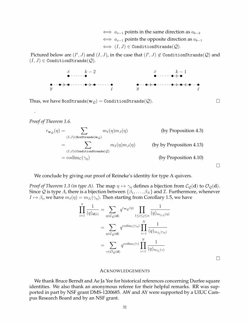
Pictured below are (I ′, J) and (I, J), in the case that (I ′, J) ∈ ConditionStrands(Q) and(I, J) ∈ ConditionStrands(Q).

y ℓ

x k − 2

y ℓ

x k − 1

Thus, we have BoxStrands(wQ) = ConditionStrands(Q). �

.

Proof of Theorem 1.6.

rwQ(η) =∑

(I,J)∈BoxStrands(wQ)

mI(η)mJ(η) (by Proposition 4.3)

=∑

(I,J)∈ConditionStrands(Q)

mI(η)mJ(η) (by by Proposition 4.13)

= codimC(γη) (by Proposition 4.10)

�

We conclude by giving our proof of Reineke’s identity for type A quivers.

Proof of Theorem 1.3 (in type A). The map η 7→ γη defines a bijection from CQ(d) to OQ(d).Since Q is type A, there is a bijection between {β1, . . . , βN} and I. Furthermore, wheneverI 7→ βi, we have mI(η) = mβi

(γη). Then starting from Corollary 1.5, we haven∏

i=1

1

(q)d(i)=

∑η∈CQ(d)

qrwQ (η)∏

1≤i≤j≤n

1

(q)m[i,j](η)

=∑

η∈CQ(d)

qcodimC(γη)N∏i=1

1

(q)mβi(γη)

=∑

γ∈OQ(d)

qcodimC(γ)N∏i=1

1

(q)mβi(γ)

�

ACKNOWLEDGEMENTS

We thank Bruce Berndt and Ae Ja Yee for historical references concerning Durfee squareidentities. We also thank an anonymous referee for their helpful remarks. RR was sup-ported in part by NSF grant DMS-1200685. AW and AY were supported by a UIUC Cam-pus Research Board and by an NSF grant.

32

REFERENCES

[ADF80] S. Abeasis and A. Del Fra. Degenerations for the representations of an equioriented quiver of typeAm. Un. Mat. Ital. Suppl, 2:157–171, 1980.

[And84] G. E. Andrews. The Theory of Partitions:. Cambridge University Press, Cambridge, 1984. ISBN9780511608650. doi:10.1017/CBO9780511608650.

[Bou02] P. Bouwknegt. Multipartitions, generalized Durfee squares and affine Lie algebra characters. Jour-nal of the Australian Mathematical Society, 72(3):395–408, 2002.

[Bou10] C. Boulet. Dysons new symmetry and generalized Rogers-Ramanujan identities. Annals of Combi-natorics, 14(2):159–191, 2010.

[BR07] A. Buch and R. Rimnyi. A formula for non-equioriented quiver orbits of type A. Journal of Alge-braic Geometry, 16(3):531–546, 2007. ISSN 1056-3911.

[Bri08] M. Brion. Representations of quivers. 2008.[DM16] B. Davison and S. Meinhardt. Cohomological Donaldson-Thomas theory of a quiver with poten-

tial and quantum enveloping algebras. arXiv:1601.02479, 2016.[FG09] V. V. Fock and A. B. Goncharov. Cluster ensembles, quantization and the dilogarithm. Ann. Sci.

Ec. Norm. Super. (4), 42(6):865–930, 2009.[FK94] L. D. Faddeev and R. M. Kashaev. Quantum dilogarithm. Modern Physics Letters A, 9(05):427–434,

1994.[FV93] L. Faddeev and A. Y. Volkov. Abelian current algebra and the virasoro algebra on the lattice.

Physics Letters B, 315(3-4):311–318, 1993.[GH68] B. Gordon and L. Houten. Notes on plane partitions. {II}. Journal of Combinatorial Theory, 4(1):81

– 99, 1968. ISSN 0021-9800.[Kel11] B. Keller. On cluster theory and quantum dilogarithm identities. In Representations of algebras and

related topics, EMS Ser. Congr. Rep., pages 85–116. Eur. Math. Soc., Zurich, 2011.[KMS06] A. Knutson, E. Miller and M. Shimozono. Four positive formulae for type A quiver polynomials.

Inventiones mathematicae, 166(2):229–325, 2006.[KS11] M. Kontsevich and Y. Soibelman. Cohomological Hall algebra, exponential Hodge structures and

motivic Donaldson-Thomas invariants. Commun. Number Theory Phys., 5(2):231–352, 2011.[Rei01] M. Reineke. Feigin’s map and monomial bases for quantized enveloping algebras. Mathematische

Zeitschrift, 237(3):639–667, 2001.[Rei10] —. Poisson automorphisms and quiver moduli. Journal of the Institute of Mathematics of Jussieu,

9(03):653–667, 2010.[Rim13] R. Rimanyi. On the cohomological Hall algebra of Dynkin quivers. arXiv:1303.3399, 2013.[Rin80] C. M. Ringel. The rational invariants of the tame quivers. Inventiones mathematicae, 58(3):217–239,

1980.[Sch53] M.-P. Schutzenberger. Une interpretation de certaines solutions de l’equation fonctionnelle-

f(x+y)= f(x)f(y). Comptes Rendus Hebdomadaires des Seances de l’Academie des Sciences, 236(4):352–354, 1953.

[SW98] A. Schilling and S. O. Warnaar. Supernomial coefficients, polynomial identities and q-series. TheRamanujan Journal, 2(4):459–494, 1998.

DEPARTMENT OF MATHEMATICS, THE UNIVERSITY OF NORTH CAROLINA AT CHAPEL HILL, CB #3250,PHILLIPS HALL, CHAPEL HILL, NC 27599

E-mail address: rimanyi@email.unc.edu

DEPARTMENT OF MATHEMATICS, UNIVERSITY OF ILLINOIS AT URBANA-CHAMPAIGN, URBANA, IL61801

E-mail address: weigndt2@uiuc.edu, ayong@uiuc.edu

33