Strategies and Procedures for Bead Optimization

Particle TechnologyTechnical Notes and Reference Guide

These technical notes offer basic strategies, guidelines,

and procedures for using and applying various types

of beads for your specific needs. You’ll find ideas for

coupling beads to proteins, sonication and mixing

beads, and selecting the right bead surface property

for diagnostic applications. You can learn more about

the importance of mean diameter and uncertainty for

effective instrument calibration, and get clarification on the

differences between the various types of flow cytometry

beads. There’s even a referesher on the basic ways for

working with and handling beads.

Sharing our knowledgeto help ensure your success

Thermo Fisher Scientific provides this manual “as is” without warranty of any kind, either expressed or implied, but not limited to, the implied warranties of merchantability or fitness for a particular purpose. Thermo Fisher shall not be liable to customers and non-customers for any claims, damages or losses incurred arising from any failure of customers and non-customers due to the information provided in this manual; any inaccuracies, errors or omissions in the statements made in this manual, and the use and reliance by customers and non-customer on such statements.

Information is current up to the date shown on the back cover of this manual. Contact your local sales representative to determine if a more up-to-date version is available. Modifications and/or improvements to the products described in this manual may be made at any time.

This manual may contain information about or make reference to products or services that are not released for sale in the customer’s country or no longer available. Such information or references shall not be construed to mean that Thermo Fisher Scientific will have such products or services available for sale in the customer’s country. Contact Thermo Fisher Scientific for further information.

All rights reserved. No part of this publication may be reproduced, transmitted, transcribed, stored in a retrieval system, or translated into any language in any form by any means without the expressed written permission of Thermo Fisher Scientific.

Disclaimer

Contents

HISTORY OF PARTICLE REAGENTS

Polystyrene-based Microparticles (PS-MPs) 5

Other Monomers 6

Cleaning Methods 6

Protein Adsorption: PS-MPs 7

TECHNICAL NOTES ON DIAGNOSTICS

Recommended Adsorption and Covalent Coupling Procedures 10

Sonication and Mixing 15

General Guidelines for Working With and Handling Particles 19

Factors Affecting Adsorption and Pre-Covalent Coupling of Protein to Particles 21

Selecting Particle Surface Properties For Diagnostic Applications 26

Particle Bound Protein Assay Quick Elution Technique 28

Derivation of Count per Milliliter from Percentage of Solids 32

Evaluating Pore Sizes of Biological Membranes with Fluorescent Microspheres 34

TECHNICAL NOTES ON QC / CALIBRATION

The Importance of Measurement Components in Instrument Calibration and Method Validation 38

Improved Array Method for Size Calibration of Monodisperse Spherical Particles by Optical Microscope 40

Calibration of Spherical Particles by Light Scattering 44

Internal Standard Method for Size Calibration of Sub-Micrometer Spherical Particles by Electron Microscope 48

Index of Refraction 51

Particle Retention Testing of 0.05 to 0.5 Micrometer Membrane Filters 52

5

The latex agglutination test was first introduced by Singer and Plotz in 1956 for the detection of rheumatoid factor (1). The latex particle fixation test was performed as a visible agglutination reaction using polystyrene microparticles (PS-MP) sensitized with adsorbed human immunoglobulin G (IgG). Microparticles (MPs) greatly improved earlier agglutination methods which relied on tanned sheep erythrocytes and other carriers (2).

Detection of agglutination by turbidimetry using spectropho-tometers (3-5) or by nephelometry (6) has extended the MP agglutination reaction to quantitative assays. Detection of haptens, such as drugs of abuse, may be accomplished by using agglutination inhibition assays (7, 8).

Microparticle agglutination assays constitute a sensitive and versatile homogeneous immunoassay system applicable to antigens or haptens in screening or quantitative assays. In more recent years MPs have also been used as carriers in enzyme immunoassay (9) and fluorescence immunoassay systems (10). The capture of dyed MPs is the basis for easy to us screening assays (11).

The term “latex” came from early research on synthetic rubber. Because of similar appearance, it has come to be synonymous with polystyrene microparticles. We will use the more accurate term “microparticles” in this manual.

POLYSTYRENE-BASED MICROPARTICLES (PS-MPS)

Polystyrene-based microparticles are negative charge-stabilized colloidal particles. The polymerization of styrene (12) is illustrated in Diagram 1. The basic ingredients initiation occurs when a sulfate free radical reacts with the double bond of a styrene monomerner.

The resulting styrene free radical reacts with additional molecules of styrene to produce high molecular weight chains of polystyrene. Chain termination occurs when two growing chains react to make a sulfate terminated polymer chain. These polystyrene chains spontaneously coalesce to form spheres due to their insolubility in water.

The sulfate groups at the chain termini are located on the surface, where they can interact with the water phase. Detergents (surfactants), which are often used in polymerization, are found both adsorbed to the MPS and free in solution.

Diagram 1

History of Particle Reagents

6

Colloidal stability, defined as maintaining separate particles, requires a minimum amount of negative surface charge. Negative charge supplies a repulsive electrostatic force to counteract the inherent attractive van der Waals force. Thermo Scientific particles are prepared by emulsion polymerization with an anionic detergent; the stabilizing negative charge on these particles is supplied by a combination of surface sulfate groups and adsorbed anionic detergent (Diagram 2).

Particles may be prepared without surfactant (so called “soap-free latex”) by increasing the concentration of initiator over emulsion polymerization conditions. This results in particles stabilized with a high density of surface sulfate and with correspondingly shorter length polymer chains.

Diagram 2

OTHER MONOMERS

PS-MPs may be modified by copolymerizing styrene with various hydrophilic monomers (Table 1). Copolymer MPs offer altered binding properties and generally increased colloidal stability. Many of the copolymers also provide chemically reactive groups for covalent coupling of protein.

These functional groups may be divided into two categories, activatable and preactivated. Activatable groups such as carboxyl require reaction with an activating chemical prior to coupling. Preactivated groups are sufficiently reactive to undergo coupling to proteins “as is”. It should also be noted that very hydrophilic particles may be prepared with methacrylates as the principle monomer (in place of styrene). Methacrylate MPs have a lower refractive index than PS-MPs.

PS-MPs prepared with hydrophilic comonomers have surface layers which are, to varying degrees, “fuzzy”. The surface of carboxylated MPs, for example, is shown by colloidal measurements to have a gel-like outer layer which is enriched in carboxylic acid (13).

Comparison of acrylic acid- and methacrylic acid-modified particles demonstrate that the more water-soluble acrylic acid interacts strongly with water at the surface, while the less water soluble methacrylic acid is partially buried in the polystyrene core (13).

Thus, the availability of a comonomer functional group at the surface varies with the solubility of the monomer. The advantages and disadvantages of having fuzzy, hydrophilic or acidic surface properties will be one of the important themes of this manual.

Table 1

CLEANING METHODS

Cleaning methods for MPs are designed to remove various ionic by-products of polymerization. These by-products, which may affect the performance of MPs, include surfactant and buffer salts.

For PS-MPs, these substances amount to about 0.2 % in a 10% solids MP suspension. When hydrophilic monomers are included in a polymerization recipe, soluble polymer chains are also formed as a by-product. These chains may be adsorbed to the surface or free in the aqueous phase and may alter the functional behavior of the MPs (14).

For hydrophilic comonomer MPs, soluble polymer may amount to 0. 3 % in a 10% solids MP suspension. As the MPs are diluted to 1 % solids or lower for coupling reactions, these substances are diluted accordingly, so that in actual coupling situations, the concentrations are very low.

7

MPs are cleaned by a variety of methods, but the two most efficient methods are ion exchange and tangential flow filtration. The various by-products in MP preparations are ionic and can be removed using suitable ion exchange resins (12). Tangential flow filtration is also an effective method for removing by-products (15).

The necessity of cleaning the MPs before use depends on the type of particle and the application. It is widely assumed that surfactants useq in emulsion polymerization will interfere with protein binding. The work of Gardas and Lewartowska demonstrates that the effect of surfactant on the binding of proteins to PS surfaces depends on the critical micelle concentration (CMC) of the particular surfactant (16).

Thermo Fisher Scientific uses detergents with a high CMC (that is, with a low tendency to form micelles) which have very little effect on protein binding. Also, in the case of plain PS-MPs, cleaning can cause destabilization (reduced. colloidal stability) by removing adsorbed surfactant.

Even MPs prepared without surfactants (“soap-free”) have the other by-products, buffer saIts and soluble polymer. These can be detected, by measuring the conductivity of the suspension compared to purified water. To obtain absolutely “pure” MPs, cleaning by one of the methods described is necessary for any microparticle preparation.

PROTEIN ADSORPTION: PS-MPS

The adsorption of proteins to PS-MPs occurs rapidly and spontaneously due to noncovalent interactions. Addition of increasing amounts of protein to a fixed mass of MP will result in a saturation binding curve due to the formation of a monolayer of bound protein (17, 18).

In some cases, kinks or steps in the binding isotherm have been observed; these are interpreted as indicating a change in the conformation of the bound protein (18). If the amount of bound protein per unit area of surface is calculated, it is seen that saturation of MPs of different diameters represents a constant amount of bound protein per unit surface area (17). The surface area of a uniform microparticle suspension may be calculated with the formula:

S= 5.71/D, where

S is surface area in meters squared per gram of MP, and

D is particle diameter in micrometers (microns).

Note that the total surface area per unit mass of particles increases inversely with the diameter. Thus, more protein is required to saturate equivalent weight suspensions of smaller diameter particles. This fact should be kept in mind when working with particles of varied diameters.

In an early study on the mechanism of adsorption of proteins to PS-MP, Singer and van Oss looked at the adsorption of radiolabelled proteins to PS-MPs (19). They concluded that IgG binds solely by hydrophobic or van der Waals forces, while the binding of human serum albumin (HSA) and hemoglobin involves electrostatic as well as hydrophobic forces.

These differences in binding were attributed to the different charge density and degree of hydration of these proteins. IgG has low charge density and a lesser degree of hydration relative to HSA and hemoglobin, meaning less work has to be done to move the water aside and obtain close contact between the protein and MP.

The binding of IgG was found to be pH independent, while the binding of HSA and hemoglobin was pH dependent. They also noted that the binding of HSA and hemoglobin was low compared to IgG, possibly because IgG is a larger molecule with a correspondingly greater van der Waals attraction.

In a study of the effects of pH on the binding of IgG to polyvinyltoluene MPs (very similar to PS-MPs), Bagchi and Birnbaum found maximum binding at pH 7.8 (the isoelectric point or pI of IgG) (20). Under their conditions of low ionic strength and no buffer, binding decreased linearly as pH was changed from the pI in either direction. The binding was thus seen to be mainly hydrophobic, since there was no evidence of increased binding below the isoelectric point where the MP is still negative but the IgG is positively charged.

The differences in amount of bound IgG at saturation (the plateau level on the binding isotherm) at different binding pH was explained by pH induced conformational changes; at pH away from pI, the IgG molecule takes on more charge and the molecule expands due to charge repulsion. This expansion of the IgG molecule results in a lower amount bound at saturation. Results of intrinsic viscosity measurements of IgG solutions support this hypothesis.

Norde and Lyklema performed detailed mechanistic studies on the binding of HSA and bovine pancreas ribonuclease (RNase) to PS-MPs (18). In this work the effects of MP surface charge (two PS-MPs of differing sulfate density were used), pH, ionic strength, and temperature were studied. HSA showed maximum binding to both MPs at its pI, in agreement with Bagchi and Binbaum (20).

8

Overall, the binding of HSA was greater to the higher charge MP. This is consistent with the data of Singer and van Oss (19), showing an ionic component in the adsorption of HSA. The binding of HSA demonstrated a complex interdependence of pH, ionic strength and particle charge density. Raising the ionic strength increased the adsorption of HSA to the higher charge MP, but had no effect on adsorption to the lower charge MP, over the same range of pH.

The binding of RNase was less affected by pH, and there was no maximum in binding at the pl. The binding of RNase to the higher charge MP decreased when the ionic strength was raised over a range of pH; this was the opposite of what was seen with HSA. The HSA molecule has high flexibility and undergoes conformational changes under different solution conditions. RNase, with a rather rigid structure, resists changes due to solution conditions. These differences in protein solution behavior were invoked to explain the observed differences in binding behavior (18).

Adsorptive binding of proteins to PS-MP involves noncovalent forces which are individually weak but become strong due to extensive contact between protein and particle surface. Thus, adsorptive binding is largely irreversible to dilution (protein does not desorb upon dilution) in the same buffer used for binding (17, 20, 21).

As Bagchi and Birnbaum describe it, “complete desorption is energetically less favorable than adsorption, because adsorption can be achieved by single contact but desorption must be accompanied with breaking of all contact points (20)”. Partial desorption of IgG from polyvinyltoluene particles was seen upon changing pH; this was attributed to conformational change in the IgG molecule (20).

Detergents are generally capable of displacing adsorbed protein (19, 22), and the displacement of a bound protein by another protein in solution can occur (22, 23). It should also be noted that if more than a single protein is in solution during binding, there will be competition for binding, based on the relative affinity of each protein for the surface (23).

The driving force for adsorption is best explained as an increase in entropy for both the protein and the water molecules displaced from the MP surface. When proteins adsorb to a solid phase, water must be “squeezed out” from between the protein and the hydrophobic surface. Therefore, the hydration of the protein or the MP surface can affect the amount of energy it takes to adsorb the protein (19).

The result of adsorption is an increase in entropy in the water molecules freed from the hydrophobic surface (24). This may be thought of as the water molecules giving up the energy it took to keep them trapped at the surface. This energy is transferred to the protein, which may rearrange at the surface and lose tertiary structure. This results in an increase in entropy for the protein molecule (18).

In summary, the factors which have been identified in the literature as affecting the adsorption of proteins to polystyrene MPs are pH, ionic strength, properties of the protein, and charge density of the PS-MPs. Most of these studies were theoretical in nature, aimed to understand mechanisms rather than to develop a product.

Often, no buffer was used. The study described in Chapters 3 and 4 of this book takes a practical approach, using buffers and ionic strength conditions consistent with maintaining the immunoreactivity of antigens and antibodies. However, the same factors are found to be important, and many of the same principles hold.

PARTICLE TECHNOLOGY

PARTICLE TECHNOLOGYTECHNICAL NOTES ON

10

Particle Reagent Optimization: Recommended Adsorption and

Covalent Coupling Procedures

The following procedure outlines the suggested materials and process for the coupling of Thermo Scientific polymer particles to proteins. These recommended coupling procedures are designed for:

• Optimal adsorption of proteins to particles

• Optimal covalent coupling of proteins to particles

• Choice of two protocols for covalent coupling

• Simplicity, efficiency, and confidence

PRINCIPLE OF PROTEIN BINDING

Proteins bind to polystyrene (PS) or carboxylate-modified (CM) particles by adsorption.

Adsorption is mediated by hydrophobic and ionic interactions between the protein and the surface of the particles. Adsorption of proteins to particles occurs rapidly due to the particle surface free energy.

Proteins may also be covalently attached to the surface of carboxylate-modified particles. Carboxyl groups on the particles, activated by the water-soluble carbodiimide 1-ethyl-3-(3-dimethylamino) carbodiimide (EDAC), react with free amino groups of the adsorbed protein to form amide bonds.

Performing covalent coupling with the direct EDAC procedure is universally useful. If exposure of a protein to EDAC is discovered to be harmful to the protein, then a pre-activation (active ester) step prior to introducing the protein is an alternative procedure for successful covalent coupling.

The following are protocols for both adsorption and covalent coupling. These protocols are written for 1.0 mL “optimization series” reactions. For larger reaction, all volumes may be scaled up proportionally.

MATERIALS AND METHODS

1. Particles

• Polystyrene particles: Thermo Scientific™ polystyrene particles for immunoassays are available in standard sizes ranging from 0.1 μm to 2.5 μm. Larger particles are also available.

These polystyrene particles are manufactured by emulsion polymerization using an anionic surfactant and have surface sulfate groups which arise from the polymerization initiator.

Thermo Scientific polystyrene particles are formulated to have low free surfactant and, generally, the surfactant used does not interfere with protein binding. It is therefore recommended that Thermo Scientific polystyrene particles be used without any preliminary cleanup.

• Carboxylate modified particles: Thermo Scientific carboxylate-modified particles are available in sizes ranging from 0.04 μm to 5.0 μm.

These carboxylate-modified particles are manufactured by the co-polymerization of styrene and acrylic acid using emulsion polymerization methods.

Carboxylate-modified particles are available in a wide range of carboxyl densities. Titration values in milliequivalents of carboxyl per gram of particles (mmoles/g, or µmoles/mg) are provided with each lot.

In addition, the calculated parking area (area per carboxyl group) is provided with each lot.

Thermo Scientific carboxylate-modified particles are formulated to have low detergent. The detergent used does not generally interfere with protein binding.

Carboxylate-modified particles may be rigorously cleaned by ion exchange with mixed bed resin or by tangential flow filtration (TFF).

Such cleaning removes various ionic byproducts, soluble polymers and buffer salts, which may affect coupling chemistry.

The need for preliminary clean-up of carboxylate- modified particles should be established on a case-by- case basis.

Note: Parking area (PA) is a parameter that allows comparison of carboxylate-modified particles of different diameters and titration values (mEq/g). It is an area of normalized density of carboxyl groups, given in Å2/ COOH. If two particles have the same PA, a particular protein molecule will “park on” the same number of carboxyl groups on the surface of either particle, and have an equivalent opportunity for covalent coupling (assuming all the carboxyls are activated).

2. BCA (Bicinchoninic Acid ) Surface-Bound Protein Assay for particles:

Note: See “Particle Bound Protein Assay Quick Elution Technique” for materials and methods.

11

3. Reaction Buffer: MES Buffer 2-(N-morpholino) ethanesulfonic acid: Prepare 10X stock buffer at 500 mM, pH 6.1. The pH will not change significantly on dilution. Store at 4°C and discard if yellow or contaminated.

4. EDAC 1-ethyl-3-(3-dimethylaminopropyl) carbodiimide hydrochloride 52 µmol/mL: Just before use, weigh approximately 10 mg of EDAC on an analytical balance. For each 10 mg weighed, add 1.0 mL of deionized water.

Note: EDAC is very sensitive to moisture and undergoes rapid hydrolysis in aqueous solutions. EDAC should be stored in a desiccator at -5°C and brought to room temperature before weighing.

5. NHS, N-hydroxysuccinamide (Active Ester-Two-step Coupling Procedure only): 50 mg/mL in water (very soluble).

6. Protein Stocks: Typically, a protein stock in the range of 1-10 mg/mL is recommended.

Note: The protein to be coated onto particles should be completely dissolved and not too concentrated.

7. Deionized (DI) water

Appropriate labware including:

• Pipettes and tips (10 µL – 5 mL)

• Mixing wheel or other device

• Microcentrifuge tubes

• Microcentrifuge

Note: Centrifuge 13,000 RPM (16,100 x g) for samples 1.0 mL or less and 15,000-17,000 RPM (22,000-29,000 x g) for samples up to 20 mL.

• Tangential flow filtration: Smaller particles may require tangential flow filtration or ultra-centrifugation for washing

Note: Tangential Flow Filtration (TFF) membrane devices are available from several suppliers in sizes suitable for processing particles in milliliter to liter quantities. Particles as small as 0.05 μm may be reliably processed with (TFF) membranes.

• Probe-type ultrasonicator: A probe-type ultrasonicator with a microtip should be used for resuspending particle pellets during washing.

Sonication is also helpful for re-dispersing clumped particles in a stabilizing buffer.

An immersible ultrasonic probe is the ideal tool for efficient resuspension of particle pellets. For 1.0 mL reactions, a few seconds of sonication is sufficient.

Alternatively, pellets may be stirred or resuspended by repeated aspiration with a fine pipette tip.

Note: Vortex mixing and bath-type sonicators are not effective for resuspending most pellets.

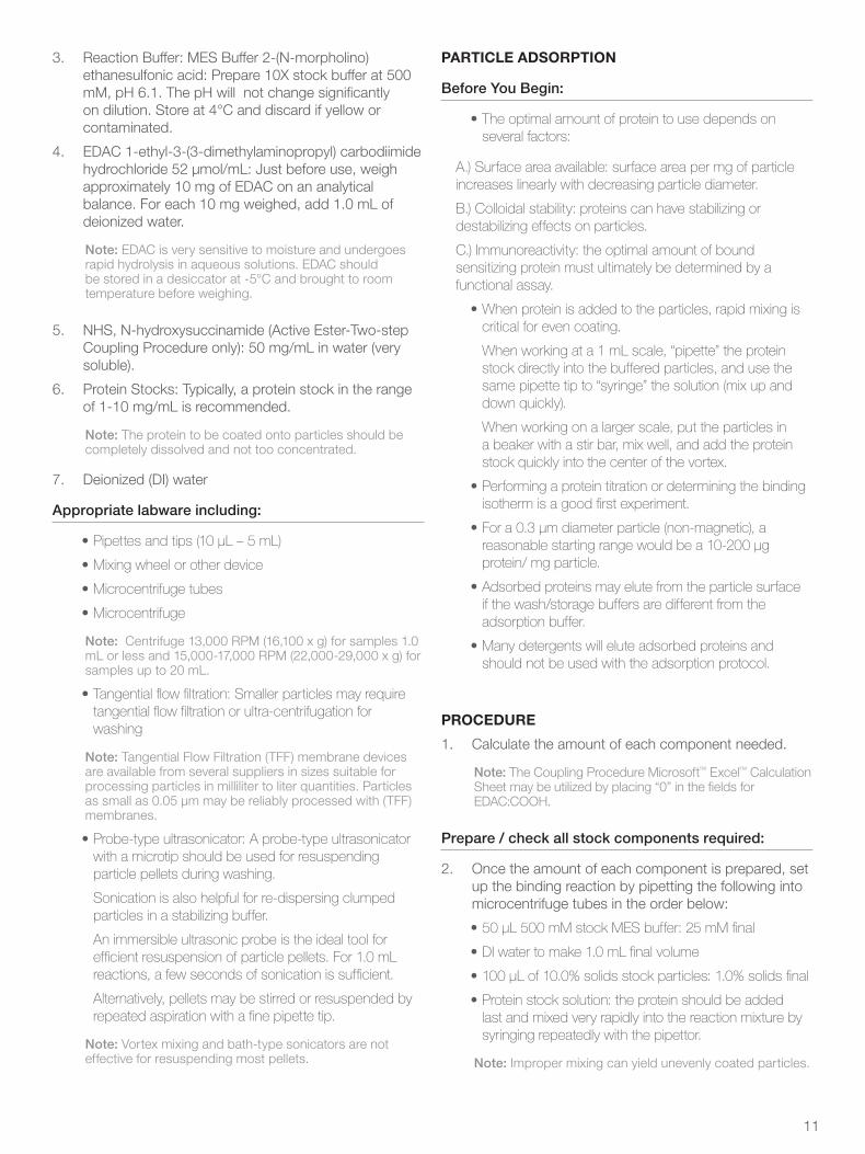
PARTICLE ADSORPTION

Before You Begin:

• The optimal amount of protein to use depends on several factors:

A.) Surface area available: surface area per mg of particle increases linearly with decreasing particle diameter.

B.) Colloidal stability: proteins can have stabilizing or destabilizing effects on particles.

C.) Immunoreactivity: the optimal amount of bound sensitizing protein must ultimately be determined by a functional assay.

• When protein is added to the particles, rapid mixing is critical for even coating.

When working at a 1 mL scale, “pipette” the protein stock directly into the buffered particles, and use the same pipette tip to “syringe” the solution (mix up and down quickly).

When working on a larger scale, put the particles in a beaker with a stir bar, mix well, and add the protein stock quickly into the center of the vortex.

• Performing a protein titration or determining the binding isotherm is a good first experiment.

• For a 0.3 µm diameter particle (non-magnetic), a reasonable starting range would be a 10-200 μg protein/ mg particle.

• Adsorbed proteins may elute from the particle surface if the wash/storage buffers are different from the adsorption buffer.

• Many detergents will elute adsorbed proteins and should not be used with the adsorption protocol.

PROCEDURE

1. Calculate the amount of each component needed.

Note: The Coupling Procedure Microsoft™ Excel™ Calculation Sheet may be utilized by placing “0” in the fields for EDAC:COOH.

Prepare / check all stock components required:

2. Once the amount of each component is prepared, set up the binding reaction by pipetting the following into microcentrifuge tubes in the order below:

• 50 μL 500 mM stock MES buffer: 25 mM final

• DI water to make 1.0 mL final volume

• 100 μL of 10.0% solids stock particles: 1.0% solids final

• Protein stock solution: the protein should be added last and mixed very rapidly into the reaction mixture by syringing repeatedly with the pipettor.

Note: Improper mixing can yield unevenly coated particles.

12

3. Mix tubes at room temperature on a mixing wheel or other device for one hour.

Note: Gentle, constant mixing is important for particle reactions.

4. Remove unbound protein: pellet particles by centrifugation and decant the supernatant.

5. Perform two washes with your buffer (this may be the MES buffer). Pellet particles by centrifugation and decant the supernatant. Resuspend pellets between washes using ultrasonication.

6. Resuspend final pellet to desired % solids with the same buffer. For example, if the target % solids is 1.0%, then add 0.97 mL of the same buffer, given that some liquid remains after pellet formation.

7. Perform the Particle Bound Protein Assay Quick Elution Technique procedure as an analytical tool to assess the amount of protein bound on the particles.

COVALENT COUPLING

Before You Begin:

1. To determine the optimal amount of EDAC concentration (EDAC:COOH) in one step covalent coupling, an EDAC titration (holding the protein constant) is performed.

Note: The Coupling Procedure Microsoft Excel Calculation Sheet may be utilized by placing ranges of concentrations in the “EDAC:COOH” fields and a constant value for the “Protein added” fields. It is recommended to use an approximate 0.5 to 2.5 fold molar excess over particle carboxyl concentration.

2. For active ester (two step coupling), the concentration of EDAC:COOH may be varied. However, the recommended molar ratio is 2.5 to 1. For NHS:COOH, the recommended molar ratio is 20 to 1.

3. Once an optimal EDAC concentration is determined, the optimal amount of protein to be added for meeting the application performance criteria needs to be determined. To do this, perform a protein titration holding the determined EDAC concentration fixed.

Note: The Coupling Procedure Microsoft Excel Calculation Sheet may be utilized by placing ranges of concentrations in the “Protein added” field and the determined optimal EDAC:COOH concentration in the “EDAC:COOH” fields.

4. The optimal amount of protein to use depends on several factors:

• Surface area available: surface area per mg of particle increases linearly with decreasing particle diameter.

• Colloidal stability: proteins can have stabilizing or destabilizing effects on particles.

• Immunoreactivity: the optimal amount of bound sensitizing protein must ultimately be determined by a functional assay.

5. Performing a protein titration or determining the binding isotherm is a good first experiment. For a 0.3 μm diameter particle (non-magnetic), a reasonable starting range would be a 10-200 μg protein/mg particle.

• When the protein is added to the particles, rapid mixing is critical for even coating. When working at a 1 mL scale, “pipette” the protein stock directly into the buffered particles, and use the same pipette tip to “syringe” the solution (mix up and down quickly).

When working on a larger scale, put the particles in a beaker with a stir bar, mix well and add the protein stock quickly into the center of the vortex.

1. For optimization scale, it is convenient to run coupling reactions in microcentrifuge tubes. With conventional microcentrifuges (i.e., Eppendorf™), coated particles of 0.150 μm or greater diameter are pelleted in 10- 30 minutes. For smaller particles of 0.150 μm or less diameter, longer centrifugation times are needed as the pellets are more difficult to resuspend.

2. Smaller particles may require tangential flow filtration or ultracentrifugation for washing.

3. Colloidal stability problems increase with decreasing particle diameter. Lowering the percent solids in the coupling step to 0.5% instead of 1% helps prevent clumping during coupling.

4. The particles may clump during coupling due to the electrostatic effect of the positively charged EDAC molecules, the effect of the protein itself, or consumption of negative charge by amide bond formation. Washing into fresh buffer to remove EDAC and unbound protein, followed by sonication, generally reverses the clumping. Long term colloidal stability of coated particles requires development of the right storage buffer.

5. The selection of storage buffer and pH is critical in achieving optimum particle performance. Zwitterionic buffers such as 3-Morpholino-2-hydroxypropanesulfonic acid (MOPSO), blocking proteins, and bovine serum albumin (BSA), along with fish skin gelatin (FSG), higher pH, detergents and sodium salicylate, have all proven to be useful for stabilizing particle preparations while permitting specific agglutination reactions to occur.

6. Blocking proteins with a high negative charge, such as BSA and FSG, may be used to add colloidal stability, as well as block the surface against nonspecific sample adsorption. FSG works especially well with antibody-coated particles.

13

ONE STEP COUPLING PROCEDURE

1. Calculate the amount of EDAC required.

Note: The “Coupling Procedure Microsoft™ Excel™ Calculation Sheet” may be utilized to perform the calculations.

Given Equations:

Equation 1: (Particle acid content) mEq/g is equivalent to μmol/mg

Note: 1 mL of 1% particles contain 10 mg particles.

Equation 2: (Acid content, µmol/mg) (10 mg particles)

(desired ratio) = μmol EDAC required

Equation 3: (μmol EDAC required)/

(52 μmol/mL) = mL EDAC stock per mL of reaction

2. Set up binding reaction by “pipetting” into microcentrifuge tubes in the order below:

• 500 mM stock MES buffer: 25 mM final

• 10.0% solids stock particles: 1.0% solids final

• Protein stock solution (add last)

3. Mix the tubes for approximately one hour on a mixing wheel at room temperature.

Note: Gentle, constant mixing is important for particle reactions.

4. Prepare the EDAC solution immediately before use and mix the calculated volume rapidly into the reaction by syringing repeatedly with the pipettor.

5. Mix tubes at room temperature on a mixing wheel or another similar device for one hour. Particles may clump during this time, but this is not unusual or harmful.

6. Remove unbound protein: pellet particles by centrifugation for carboxylate-modified particles, and decant the supernatant.

7. Perform two washes with your buffer (this may be the MES buffer or a higher pH buffer of your choice). Pellet particles by centrifugation for carboxylate-modified particles, and decant the supernatant. Resuspend pellets between washes by ultrasonication.

8. Resuspend final pellet to desired percentage solids with buffer that does not contain blocking proteins. This may be the MES buffer or a higher pH buffer of your choice. For example: if the target % solids is 1.0%, then one would add 0.97 mL of the same buffer, given that some liquid remains after pellet formation.

9. Perform the Particle Bound Protein Assay Quick Elution Technique as an analytical tool to assess the amount of protein bound to the particles.

10. For long term colloidal stability, a stabilizing storage buffer will be needed. After performing the protein analysis, coated particles can be pelleted and re-

suspended in a variety of storage buffers, and the colloidal stability and reactivity optimized.

Note: Covalently bound protein will not elute when subjected to detergent washes or buffer changes. As a result, covalently coupled reagents are compatible with a wider variety of buffer additives than reagents where the proteins are only adsorbed to the particles.

ACTIVE ESTER TWO STEP COUPLING PROCEDURE

Step One: Pre-activation

1. Pipette into microcentrifuge tubes in the order below:

• 100 μL of 500 mM MES buffer: 50mM final

• 100 μL of 10.0% solids stock particles: 1.0% solids final

• 230 μL NHS solution: 100 mM final

• EDAC solution, calculated amount

• Water to make 1.0 mL final volume

2. Mix tubes at room temperature on a mixing wheel or another similar device for 30 minutes.

Note: Gentle, constant mixing is important for particle reactions.

3. Pellet particles by centrifugation for carboxylate- modified particles, and decant the supernatant.

4. Resuspend particles with 1 mL 50 mM MES buffer, pH 6.1.

5. Pellet particles by centrifugation for carboxylate- modified particles, and decant the supernatant.

6. Resuspend the pellet by adding the following and sonicating:

• 100 μL 500 mM MES buffer: 50 mM final

• Water to make 1.0 mL final volume

Step Two: Protein Coupling

1. Add the protein stock solution.

2. Mix tubes at room temperature on a mixing wheel or another similar device for 1 hour.

Note: Gentle, constant mixing is important for particle reactions.

3. Remove unbound protein: pellet particles by centrifugation for carboxylate-modified particles, and decant the supernatant.

4. Wash with your 50mM buffer (this may be the MES buffer or a higher pH buffer of your choice).

5. Pellet the particles by centrifugation for carboxylate- modified particles, and decant the supernatant.

6. Resuspend pellets between washes by ultrasonication.

7. Repeat steps 4-6, for a total of 2 washes.

14

After performing the protein analysis, coated particles can be centrifuged and resuspended in a variety of storage buffers, and the colloidal stability and reactivity optimized.

Note: Covalently bound protein will not elute when subjected to detergent washes or buffer changes. As a result, covalently coupled reagents are compatible with a wider variety of buffer additives than reagents where the proteins are merely adsorbed to the particles. IgG profoundly destabilizes microparticles. With higher IgG load the aggregation and settling is quicker. Raising the pH of your buffer can help considerably. Getting the pH above 8.0 often makes a major difference. The average isoelectric point (pI) of IgG is about 7.9. Above the pI the net charge of the IgG becomes negative and that helps to stabilize the particles. Tris is a suitable buffer for pH of 8 and up. You could take several aliquots of current preps and centrifuge wash them into alternate buffers with higher pH: ~8.5, or Tris buffer for the HEPES could be used. Then let these preps stand and watch for settling. Another additive of value that is not widely known is sodium salicylate. This can be added at concentrations of 50 to 100 mmol/L. Sodium salicylate has a negative charge and adsorbs to the microparticle surface via the benzene ring. This then provides negative charge stabilization. Note that the sodium salt must be used as the protonated acid form is very hard to dissolve.

15

Particle Reagent Optimization: Sonication and Mixing

INTRODUCTION

Processing particles is one of the most critical phases in particle technology, and having guidance on the use of sonication will simplify your process. For your benefit, we have new ways to utilize our particle products and services. They are designed and engineered to meet the productivity requirements of multiple industries such as diagnostics, genomics, and proteomics.

SONICATION

Sonication provides a way to resuspend the particles thoroughly and efficiently without harm to the reagents. After centrifugation, processing steps, and coupling reactions, difficulties that arise from improper particle resuspension can be avoided by using sonication.

We routinely sonicate our coated particle preparations with a probe-type ultrasonicator to resuspend pellets after centrifugation, and to reverse mild aggregation induced by coupling. We have not found this to be detrimental to sensitized particles in any way, and have even seen improvement in sensitivity after sonication. However, sonication may prove to be detrimental to ligand coupled particles. Therefore, we recommend vortexing slowly if sonication is not desired.

It is advisable to guard against temperature rise during sonication in sensitive systems.

Using HSA/anti-HSA as a model system, we tested whether sonication caused desorption of proteins or loss of functional activity. We subjected particle reagents to full power sonication. Prolonged sonication did not result in measurable loss of HSA from the particle surface.

From our experience, it has proven to be virtually impossible to damage our plain sulfate particles with sonication or heat. In certain instances, we took the plain unbound particles to the boiling point and did not observe any ill-effects. This does not apply if you have ligands bound to the surface of the particle. While the particles will survive, surface ligands could be lost.

In the process of optimization of the following procedure, one should consider the characteristics of the ligand and adjust the time and handling to ensure ligand activity.

MATERIALS

1. Effective sonicator: An immersible ultrasonic probe is the ideal tool for efficient resuspension of particle pellets. Vortex mixing and bath-type sonicators are not effective for resuspending most particle pellets.

2. Appropriate sonicator probes: A key factor that effects optimal performance of sonication is the sonication probe. The volume to be sonicated should be considered when selecting the proper probe. For example, for samples with volumes of 500 mL or less, or samples in a 1 L narrow-mouth container, we typically use a tapered micro-tip (1/8 inch diameter). For samples greater than 500 mL that are not in a narrow mouth container, we typically use a macro-tip probe (1/2 inch diameter).

3. Container for sonication: If the volume of material is 1 L or less, then the material may be sonicated in the bottle or transferred to a beaker. If a sample is greater than 1 L and in a narrow-mouth container, it needs to be transferred to an appropriate size beaker before sonication. Typically, sonication is more effective in a glass container than a plastic one.

4. Optical microscope and necessary supplies: Capable of 400X magnification.

PROCEDURE

1. Handling particles before sonication: For efficiency, the material should be thoroughly mixed before sonication. This is done by rolling the bottles of material using a mechanical roller or an overhead mixer for bulk material.

2. Select sonication intensity: For volumes using the micro-tip probe, the intensity is set between 30% and 40%, or a setting from 3 to 4 on a scale of 10. For volumes using the macro-tip probe, the intensity is set to 50%, or 5 on a scale of 10.

3. Select sonication time: Material being sonicated with the micro-tip probe is exposed for the following times according to fluid volume:

16

10 to 50 mL 20-30 seconds

50 to 100 mL 30-45 seconds

100 to 1000 mL 60-90 seconds minimum

Note: When sonicating smaller samples, the solution heats more quickly due to less volume being available to disperse the heat. For materials of 10 mL or less, a vortex mixer is recommended for resuspension. Material being sonicated with the macro tip probe is exposed for the following times according to fluid volume:

1 L 5 minutes

3 L 5 to 10 minutes

Greater than 3 L Up to 20 minutes

4. Mixing particles during the sonication process: When sonicating, it may be necessary to mix larger samples as they sonicate, or if the material tends to settle quickly out of solution, the larger samples can be sonicated, using more repetitions in shorter time frames. For example, do this when working with particles greater than 1 µm, or if the material is excessively clumped:

• If sonication of material is in a 1 L bottle, the bottle with material is rolled for five minutes between sonications, with increments of 10 minutes.

• If sonication of non-magnetic material is performed in a beaker, a magnetic stirrer is recommended to keep any aggregates in solution during sonication.

5. Observe dispersity of particles: After sonicating for a set amount of time, the material should be thoroughly mixed and observed under a microscope at 400X. When in focus, one should see a uniform distribution instead of clumps. If you see aggregates, then the material is not monodispersed. Repeat sonication and perform observation until you see no clumps.

(Top Left) Severe clumping, (Bottom Left) Light clumping, (Above Right) Well-dispersed particles

MIXING

When handling particles, it is best to mix the material to ensure it is monodispersed and uniformly distributed.

Particles may be mixed according to the type of particle and volume, using various equipment, including an overhead mixer, magnetic stirrer, vortex mixer and roller mixer.

An overhead mixer is typically used for pooling, diluting, and handling large batches.

A vortex mixer can be used for mixing product stored in small containers such as 15 mL bottles, or other applications where the container is a similar size.

The roller mixer is used to resuspend, if necessary, and uniformly mix the particles. Magnetic stirrers are used for the purpose of making a uniform mixture rather than for resuspending.

Before Starting

1. If higher than normal levels of surfactant are in the solution or if excessive foaming is observed in any of the mixing techniques, reduce the speed and time of mixing accordingly to minimize the impact on the product.

2. When resuspending material, visually confirm if possible that resuspension is complete by checking the bottom of the container for unsuspended material.

MIXING BY ROLLER MIXER

The roller mixer has a motor-driven horizontal cylinder adjacent to a free-turning horizontal cylinder that together forms a cradle on which containers of product can be placed.

The placement of the free-turning cylinder can be adjusted to accommodate different sized containers.

Use a roller mixer of sufficient size and speed for the container being mixed.

Mixing Time

Since the speed of the mixer is constant, mixing time is the way to control sufficient mixing. Mixing time can also vary based on the diameter of the container.

Since small diameter containers rotate faster than large diameter containers, mixing is accomplished more quickly.

17

Mixing time can also vary on the size of the particles. Larger particles may take more time to resuspend. Higher concentrations of particles also require more mixing time.

Note: Containers must be at least 50% and less than 90% full to have enough material covering the bottom of the container when rolling, yet not too full to prevent insufficient mixing. Extending the mixing time is acceptable. However, nothing needs to mix longer than 72 hours.

Table 1. Minimum Mixing Times Using the Roller Mixer

Container Size Particle Size (μm)

≤ 0.4 > 0.4≤1 L 10 min 40 min

>1 L 30 min 60 min

Table 1 provides guidelines for minimum mixing time according to particle and container size

MIXING BY VORTEX MIXER

A vortex mixer is used for mixing small volumes of 10 mL or less by holding the container of solution in a rubber holder and allowing a motor to rotate the shaft in an oscillating motion that causes the solution to be mixed.

Different vortex mixer models have different methods of being activated. Most have a continuous action and a manual pressure activated system. The continuous mode is generally preferred for longer vortexing times while the manual pressure mode is preferred for shorter mixing times. A vortex mixer with adjustable speed setting is recommended.

Mixing Speed

When using the controller on the mixer, adjust the speed of the mixer to a speed sufficient to cause good mixing (usually around 80% of full speed). Going too fast makes the container difficult to control.

Mixing Time

Mixing can usually be completed in 30 seconds. However, larger particles such as 0.8 and 1.0 µm require longer mixing of at least 1 minute or longer to resuspend, especially if the product has been stored for an extended period of time.

Verification of Mixing

Verify that the mixing is completed by observing the product during mixing to ensure adequate agitation. After mixing, make sure no product remains settled on the bottom of the container. Clumps should not be observed in the suspension under a microscope at 400X.

MIXING BY OVERHEAD MIXER

An overhead mixer consists of a speed controllable, electrical or air-driven motor with an agitator blade and shaft attached. Choose an overhead mixer with sufficient capability to mix the volume as required. The range of volumes is dependent on the proper agitator (i.e., a short- shafted agitator for smaller volumes).

1. Be sure that the container is such that the blade will be covered with enough product to prevent splashing

2. Position the blade high enough on a stand to allow clearance of the container (but not so high as to prevent sufficient submersion of the agitator). Best results are usually obtained when the agitator blade can be placed at a position in the lower third of the container

Mixing Speed

The proper mixing speed can be determined by observing the action of the solution. If there is no visible movement of the product, increase the speed of the mixer until there is visible movement.

In most circumstances, overhead stirring is used to achieve or maintain a uniform mixture, therefore mixing speed is not critical, as long as sufficient motion is maintained.

If one is removing aliquots from the mixture, then carefully monitor the level of product being mixed and periodically reduce the speed of the mixing to keep the product from splashing on the side of the container as the volume changes.

Mixing Time

If mixing is for the purpose of resuspension, then follow the guidelines in Table 1-Minimum Mixing Times Using the Roller Mixer.

MIXING BY MAGNETIC STIRRER

A magnetic stirrer consists of a variable speed motor with an attached magnetic rotor encased in a platform.

The rotor causes a magnetic stir bar placed in the solution to spin and mix the solution.

Select a stirrer with sufficient power to move the volume of solution and hold the container on the stirrer.

18

1. Effective mixing requires matching the container size with the volume of the solution and selecting a suitable stir bar large enough to effectively move the solution, but not so large as to cause splashing. The size of the container is determined by the size of the batch and taking several factors into account. Too large a container can cause splashing and loss of yield due to increased surface area. Containers should have a volumetric working range of 20 to 80%, and have a flat bottom that allows the stir bar to spin freely.

2. Select an appropriate sized magnetic stir bar that will fit the container and thoroughly move the volume when stirred.

Mixing Speed

Adjust the stirring speed to create enough movement of the suspension for it to be adequately mixed.

Sufficient movement ranges from creating a “dimple” 1/4-inch into the surface to a funnel shape extending approximately one-fourth of the way into the suspension.

Because the mixing is intended to evenly distribute the material in the suspension, it is not necessary to rapidly mix the suspension. However, slightly faster mixing could be required for large particles.

Avoid splashing the material. If the volume decreases, then mixing should decrease. As the volume decreases, simply reduce the mixing speed to reduce splashing.

Mixing Time

The length of time for mixing will vary with the size of the batch, i.e., the larger the batch the longer the mixing time.

However, mixing should not take longer than 30 minutes unless resuspension is the purpose of the mixing.

If mixing is for resuspension, then follow Table 1-Minimum Mixing Times Using the Roller Mixer.

19

General Guidelines for Working With and Handling Particles

PARTICLE HANDLING TIPS

The following general guidelines provide helpful tips when using our particles and should be followed accordingly.

Be sure to read the literature that accompanies your product for special handling guidelines (if any). If you have a critical application or are looking for a product that can be used without additional processing, please contact our technical service department.

Note: For most applications, it is imperative to ensure the cleanliness of diluents, sampling implements, and any other component that will make contact with the particles.

RESUSPENSION

Polymer particles ≥ 0.5 μm in suspension will settle down over time. To resuspend the particles, simply invert the bottle several times. Avoid rigorous agitation as any bubbles formed may result in statistical artifacts. Sonication after resuspension is recommended to de-gas and break up temporary agglomerates.

For applications that require the particles to be suspended for an extended period of time, a clean magnetic stir bar may be used.

DILUTION

Most particle suspensions are suitable for dilution and do not require additional surfactant/dispersant. However, the diluted suspensions should be used immediately as the stability may be affected.

1. Calculate the quantity of particles needed based on desired final concentration and quantity.

2. Resuspend the original particle suspension.

3. Transfer immediately into a clean container.

4. Add deionized water to desired amount.

SUSPENDING DRY PARTICLES

This procedure outlines the steps necessary to put a dry powder into suspension.

1. Wet the dry particles with a 1% surfactant solution (anionic or non-ionic, i.e., Tween™ 20 or Triton™ X-100) or an alcohol such as methanol or ethanol.

2. Add Deionized water to the desired amount.

DRYING A SUSPENSION

Drying a suspension to achieve a dry powder is not recom-mended. The particles may form permanent aggregates and be aerosolized, creating an inhalation hazard.

DISSOLVING POLYSTYRENE PARTICLES

In general, aromatic hydrocarbons will dissolve polystyrene. Some commonly used solvents for this application are:

1. Benzene

2. Methyl ethyl ketone (MEK)

3. Toluene

Note: MEK and toluene will dissolve polystyrene divinylbenzene (PSDVB) over time.

REMOVING/REDUCING ADDITIVES BY ION EXCHANGE OR DIALYSIS

These procedures are used to achieve low or surfactant- free suspensions. Please note that removing the surfactant from a suspension may compromise the stability of the product and should be performed immediately prior to use. Please contact us if you are looking for a low or surfactant-free product.

ION EXCHANGE

This procedure is recommended for removing ionic surfactants from the suspension and surface of the particles:

1. Obtain mixed bead ion-exchange resin (i.e., Bio-Rad™ AG501-X8).

2. For a 15 mL bottle of particles at 1% solids, use 3-4 gms of resin.

3. Wash the resin thoroughly to remove potential contaminants.

• Wash resin with approximately 200 ml deionized water.

• Allow resin to settle and then slowly pour off the water.

• Repeat above steps for a total of 5 washes.

20

4. Add the particle suspension to the resin in a small bottle. Add extra water if needed.

5. Roll the mixture for 4-6 hours and filter through washed glass wool to remove the resin.

DIALYSIS

This procedure is recommended for removing surfactants from the suspension (but not from the particle surface).

1. Wash the dialysis tubing (i.e., Spectra/Por™ 12,000-14,000 molecular weight cut-off) thoroughly with deionized water and place it in a container of deionized water (submerged).

2. Keep refrigerated for storage.

3. When ready to use, cut off the desired length of tubing

4. Place a clamp on one end or tie it off.

5. Fill about half full with the particle suspension.

6. Clamp or tie the top end and place in the container of deionized water with at least 10 to 20 times the volume of the latex.

7. Roll or stir the contents of the container.

8. Allow to dialyze for at least 4 hours.

9. Repeat dialysis three times with fresh water.

21

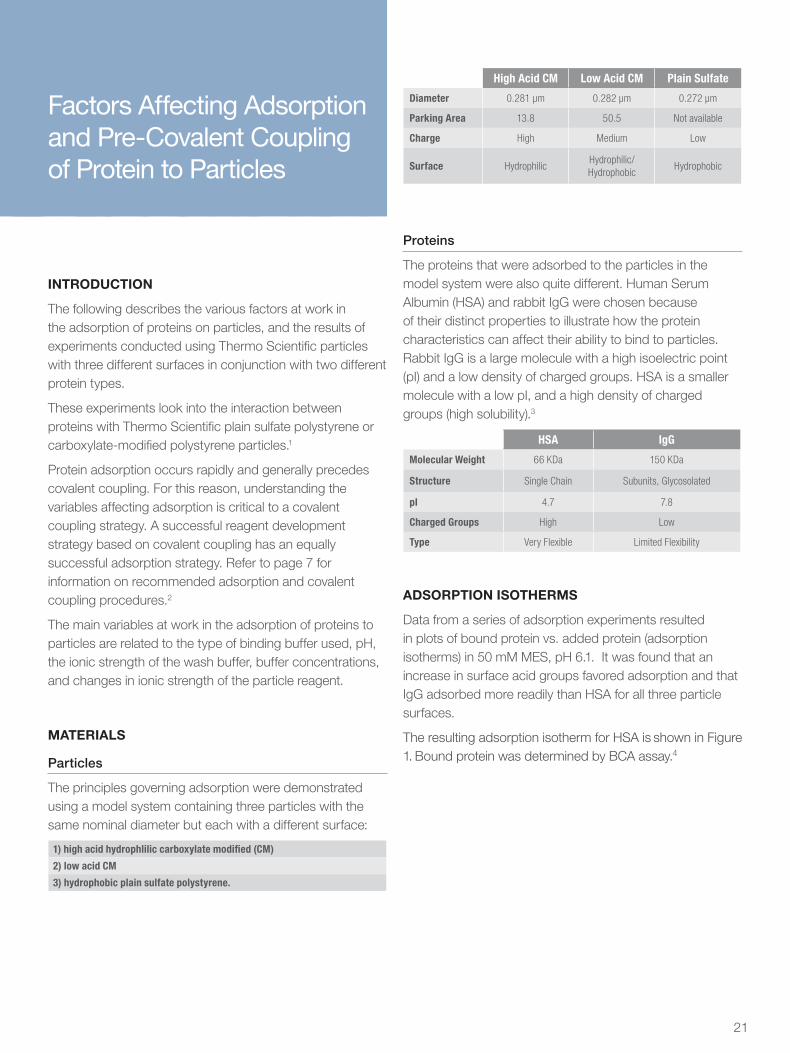
Factors Affecting Adsorption and Pre-Covalent Coupling of Protein to Particles

INTRODUCTION

The following describes the various factors at work in the adsorption of proteins on particles, and the results of experiments conducted using Thermo Scientific particles with three different surfaces in conjunction with two different protein types.

These experiments look into the interaction between proteins with Thermo Scientific plain sulfate polystyrene or carboxylate-modified polystyrene particles.1

Protein adsorption occurs rapidly and generally precedes covalent coupling. For this reason, understanding the variables affecting adsorption is critical to a covalent coupling strategy. A successful reagent development strategy based on covalent coupling has an equally successful adsorption strategy. Refer to page 7 for information on recommended adsorption and covalent coupling procedures.2

The main variables at work in the adsorption of proteins to particles are related to the type of binding buffer used, pH, the ionic strength of the wash buffer, buffer concentrations, and changes in ionic strength of the particle reagent.

MATERIALS

Particles

The principles governing adsorption were demonstrated using a model system containing three particles with the same nominal diameter but each with a different surface:

1) high acid hydrophlilic carboxylate modified (CM)

2) low acid CM

3) hydrophobic plain sulfate polystyrene.

High Acid CM Low Acid CM Plain Sulfate

Diameter 0.281 µm 0.282 µm 0.272 µm

Parking Area 13.8 50.5 Not available

Charge High Medium Low

Surface HydrophilicHydrophilic/ Hydrophobic

Hydrophobic

Proteins

The proteins that were adsorbed to the particles in the model system were also quite different. Human Serum Albumin (HSA) and rabbit IgG were chosen because of their distinct properties to illustrate how the protein characteristics can affect their ability to bind to particles. Rabbit IgG is a large molecule with a high isoelectric point (pI) and a low density of charged groups. HSA is a smaller molecule with a low pI, and a high density of charged groups (high solubility).3

HSA IgG

Molecular Weight 66 KDa 150 KDa

Structure Single Chain Subunits, Glycosolated

pI 4.7 7.8

Charged Groups High Low

Type Very Flexible Limited Flexibility

ADSORPTION ISOTHERMS

Data from a series of adsorption experiments resulted in plots of bound protein vs. added protein (adsorption isotherms) in 50 mM MES, pH 6.1. It was found that an increase in surface acid groups favored adsorption and that IgG adsorbed more readily than HSA for all three particle surfaces.

The resulting adsorption isotherm for HSA is shown in Figure 1. Bound protein was determined by BCA assay.4

22

Figure 1: Adsorption of HSA

All three particles reached a plateau or saturation level where adding more protein would not result in more bound protein.

A comparison of the three particle surfaces revealed a difference between the plain sulfate particle and the two carboxylated particles, and between the low acid and high acid carboxylate modified particles (Figure 1).

It is apparent that the IgG adsorbed more readily to particles than HSA for all particle surfaces (Figure 2). Both carboxylated particles adsorbed almost equal amounts of IgG and significantly more IgG than plain sulfate particles.

Figure 2: Adsorption of IgG

BINDING BUFFER TYPE AND PH

The effect of different types of binding buffers and pH on the adsorption of IgG and HSA was also studied.

In the HSA experiment (Figure 3), HSA was added at 1 mg/mL or 100 μg/mg particle. The maximum adsorption seen was 44 μg HSA/mg particle on the high acid carboxylated modified particle, which demonstrates low binding efficiency.

Figure 3: Effect of pH and Buffer on HSA Adsorption

In the IgG experiment (Figure 4), IgG was added at the same concentration as for HSA: 1 mg/mL or 100 µg/mg of particle. However, the adsorption was far more efficient, with binding of up to 95 µg IgG/mg particle on the high acid particle.

Figure 4: Effect of pH and Buffer on IgG Adsorption

Of the conditions tested, the 25 to 50 mM MES buffer at pH 6.1 yielded the highest efficiency binding of HSA and IgG on all three particles. Using any other buffers/pHs results in lower protein binding efficiency.

These studies indicate a general trend of decreasing adsorption with increasing pH. As the pH increases, the charge on the entire system becomes more negative.

PH OF WASH BUFFER

Changing the pH of the wash buffer after adsorption can result in elution of bound protein, the extent of which depends on the properties of the bound protein and particle surface.

23

To illustrate this, HSA (1 mg/mL) was adsorbed to each particle using 25 mM MES buffer. At pH 6.1, we observed the highest efficiency of HSA binding (Figure 5). After mixing for 1 hour, the coated particles were centrifuged and resuspended in 1 mL 50 mM MES at pH 6.1.

From this, 250 µL were transferred to three “fresh” tubes. The particles were pelleted and resuspended in 0.5 mL of the three buffers indicated in Figure 5.

Figure 5: Elution of Adsorbed HSA with Increasing pH

After incubating overnight at room temperature, the particles were pelleted, washed, and resuspended in 250 μL 50 mM MES at pH 6.1.

In a separate experiment, IgG (1 mg/mL) was adsorbed to each particle using 50 mM MES buffer, pH 6.1. Subsequent treatment and assay were performed exactly as described for the experiment with HSA. Results are shown in Figure 6.

Figure 6: Elution of Adsorbed IgG with Increasing pH

For both proteins, adsorption was most stable to pH changes on the plain sulfate particles. Increasing pH caused elution of protein from the low acid carboxylate

modified particle and significant elution from the high acid carboxylate modified particle.

If the eluted fraction reflected the proportion of the adsorption, which is due to electrostatic or ionic interaction, then it appears that the increased protein binding due to electrostatic forces was easily disrupted by changing the pH.

BUFFER CONCENTRATION

The effect of MES buffer concentration at pH 6.1 on HSA and IgG adsorption is shown in Figures 7 and 8, respectively.

The first point on each figure represents “0” MES, or adsorption in deionized water (pH neutral).

Figure 7: Effect of MES Concentration on HSA Adsorption

Figure 8: Effect of MES Concentration on IgG Adsorption

24

HSA was adsorbed to the three particles at 1 mg/mL added protein and varying concentrations of MES from a 500 mM stock at pH 6.1. The final pH did not vary much over this range of concentrations. The HSA-particles were washed and resuspended in 50 mM MES at pH 6.1, and the bound protein was determined by BCA assay.

IgG was adsorbed to the three particles at 1 mg/mL added protein and varying concentrations of MES from a 500 mM stock at pH 6.1 (Figure 8). The particles were washed, resuspended and assayed as previously described for HSA.

Figure 9: Effect of Ionic Strength on Adsorption of HSA

In water, the adsorption was protein and particle dependent. Where the adsorption was mainly ionic (high acid carboxylate modified particle, HSA), any buffer strength was detrimental.

Where there was some contribution to adsorption by hydrophobic attraction (low acid carboxylate modified particle or plain sulfate polystyrene, HSA; plain sulfate polystyrene, IgG), some buffer strength was advantageous. However, after a certain point, the effect of buffer strength was minor.

MES buffer concentration alone had a negative effect on adsorption to the high acid CM particle while the effect on the low acid CM particle was intermediate.

IONIC STRENGTH

The effects of ionic strength on HSA and IgG adsorption was also studied by varying the NaCl concentration in 50 mM MES, pH 6.1. HSA was adsorbed to the three particles at 1 mg/mL added protein, 50 mM MES buffer, pH 6.1 and varying concentrations of sodium chloride.

In Figure 9, the largest effect was seen with the high acid carboxylate modified particle, which showed a steady decline in HSA adsorption with increasing ionic strength from NaCl.

On the low acid carboxylate modified particle, there was a significant effect of increasing ionic strength up to 200 mM NaCl, then only a slight decline.

On the plain sulfate particle, there was only a minor effect of ionic strength on adsorption of HSA.

In Figure 10, another large effect of increasing ionic strength was seen with the high acid CM particles with a sharp drop- off in IgG adsorption above 50 mM NaCl. Adsorption to both the low acid CM particles and the plain sulfate particles was level at 100 mM NaCl, and then gradually declined.

It should be noted that the buffer concentration effects appear to be purely ionic strength effects, as the curves for increasing MES buffer concentration in Figures 7 and 8 can be overlaid on the added salt curves in Figures 9 and 10.

Figure 10: Effect of Ionic Strength on Adsorption of IgG

SUMMARY

The data in this technical note provides insights into the factors that influence protein adsorption to particles.

To relate the ionic strength effects back to the adsorption isotherms (see Figures 1 and 2), it appears that the “extra” adsorption of HSA to the high acid carboxylate modified particle was due to an ionic interaction of the amino groups of the protein to the carboxyl-rich particle. This binding was considerably reduced by high ionic strength.

25

On the low acid CM particle which adsorbed an intermediate amount of HSA, the adsorption of HSA was a combination of hydrophobic and salt-reduced ionic interactions.

On the plain sulfate particles which adsorbed the least HSA, the adsorption of HSA was predominately hydrophobic or not affected by salt.

The binding of IgG exceeded the binding of HSA onto all three particles, and more IgG was bound to the CM particles than the plain sulfate particles. The nature of IgG binding was different than that for HSA, as shown by the patterns of elution with increasing pH.

In Figure 10, another large effect of increasing ionic strength was seen with the high acid CM particles with a sharp drop- off in IgG adsorption above 50 mM NaCl. Adsorption to both the low acid CM particles and the plain sulfate particles was level at 100 mM NaCl, and then gradually declined.

For IgG, the hydrophobic component was greater and the electrostatic component was smaller. Also, the larger size of IgG compared to HSA may explain why it was more difficult to elute IgG from the plain sulfate particles.

Several key points can be taken from the adsorption experiments:

• The saturation level for a protein on a particle is important information to be gained from doing a protein binding isotherm

• MES buffer at pH 6.1 gave maximum adsorption for HSA and rabbit IgG on all three particle types tested

• Both ionic and hydrophobic forces played a role in adsorption of proteins to the particles

• The CM particles adsorbed more protein than the plain sulfate particles

• Increased protein binding due to electrostatic forces was easily disrupted by changes in pH

• The binding of IgG exceeded the binding of HSA on all three particle types used in the experiments

It is important to understand these phenomena and the complexity of the interactions between proteins and particles.

Both ionic and hydrophobic forces play a role, but individual protein characteristics sometimes make it difficult to predict the results without doing the actual experiments.

For both HSA and IgG, the same conditions (25 to 50 mM MES at pH 6.1) gave the most efficient adsorption, resulting in less waste of precious proteins. However, these conditions are not recommended for storage and use of particle reagents.

Also, if one changes the buffer, there is a risk of desorption or elution of protein.

For these reasons, we recommend using covalent coupling because it provides high efficiency coupling and the ability to change the storage/reaction buffers as desired to optimize your particle reagent.

REFERENCES

1. Griffin, C., Sutor J., Shull B., Microparticle Reagent Optimization, Seradyn Inc., Indianapolis, IN, 1994

2. Particle Reagent Optimization-Recommened Adsorption and Covalent Coupling Procedures, TN- 02702, Thermo Scientific, Fremont, CA, 2010

3. The Practical Handbook of Biochemistry and Molecular Biology, CRC Press, Boca Raton, FL, 1989

4. Particle Bound Protein Assay Quick Elution Technique, TN-2005.1_11/10, Thermo Scientific., Fremont, CA, 2010

26

Selecting Particle Surface Properties for Diagnostic Applications

Polymer particles are used in diagnostics for lateral flow chromatographic strip tests, latex agglutination assays, suspension array tests, and nephelometric assays.

There are wide variations in particle composition, surface properties, and size control that can affect the performance of a diagnostic reagent, which is why it is important to gain a better understanding of the particle selection process.

THE IMPORTANCE OF PARTICLE SURFACE PROPERTIES

The surface of particles is one of the most important properties for particles used in diagnostic tests and other applications where proteins and other biomolecules are bound to the surface.

Residual surfactants, monomers and microbial contamination can interfere with the successful conjugation to the particles. These contaminants are often the cause of batch-to-batch non-reproducibility of the conjugation reactions, and these variations can interfere with the production process for diagnostic tests.

Careful control of the particle diameter is also important since the surface area changes exponentially with the changing diameter. Variations in surface area can cause apparent changes in sensitivity. Consistency in particle manufacturing and quality control assures that these problems will not occur.

The functional groups available on the surface of the particles control the chemistry of the conjugation process and directly influence sensitivity and stability.

Selecting particles with the appropriate surface and quality characteristics is the key to developing stable, reproducible diagnostic tests.

In this section, we will discuss how surface properties affect two broad categories of biomolecular conjugation.

PROPERTIES AFFECTING HYDROPHOBIC ADSORPTION

Particles with sulfate and carboxyl groups are designed for hydrophobic (passive) adsorption.

The particle surface is very hydrophobic, with a low density of negatively charged surface ions to provide charge stabilization.

These particles will bind to any molecules that are characteristically hydrophobic, including proteins, peptides, and small hydrophobic molecules.

The binding affinity tends to increase as molecular weight increases, and can result in the preferential binding of higher molecular weight proteins in mixtures.

Specific adsorption of substances such as antibodies is easily accomplished by mixing the particles and the protein together at an optimal pH and then separating the unbound protein from the solid phase, usually by centrifugation or cross-flow filtration.

The charge groups on these particles are derived from the initiators used in the synthesis of the particles, resulting in either sulfate or carboxyl ionic groups on the particle surface.

The main difference between these two types of hydrophobic particles is their pH stability. Sulfate particles are stable above pH 3, while carboxyl particles are stable above pH 6.

There are other more subtle differences, and these come into play when one or the other particle types give a superior result when antibody is bound to its surface.

Binding, storage and reaction buffer conditions are particularly important parameters that must be optimized.

PROPERTIES AFFECTING COVALENT COUPLING

Carboxylate-modified and aldehyde-modified particles are designed for covalent attachment by reaction with amines.

The modified particles are made from sulfate particles by grafting a copolymer containing the desired chemical group onto the surface, producing a thin, relatively hydrophilic polymeric layer.

This results in a high density of carboxyl or aldehyde surface groups that can be chemically activated to give a reactive intermediate that will couple with amines on proteins and other biomolecules.

27

Carboxylate-modified particles differ from the hydrophobic carboxyl particles in that the surface is somewhat porous, more hydrophilic, and has a relatively high charge density of 10-125 Å2 /carboxyl.

These particles are more stable in the presence of high concentrations of electrolytes (up to 1 M univalent salt).

Unlike the hydrophobic carboxyl particles, the high density and better availability of the carboxyl groups on these particles facilitate reaction with protein amines after activation with carbodiimide reagents.

Alternatively, one can convert to the active esters in a two-step coupling reaction process. See page 13 for our recommended coupling procedure.

Aldehyde-modified particles have aldehyde groups grafted to the surface and can react with protein amines through Schiff base formation.

The aldehyde-modified particles do not require chemical activation and thus offer a convenient one-step method of covalent attachment.

Amine-modified particles are prepared from carboxylate- modified particles by converting some of the carboxyl groups to amine groups.The resulting amine modified particles still retain a net negative charge to ensure good charge stability, and can easily be coupled to antibodies and other proteins using a variety of bifunctional linkers.

This conjugation approach offers a different way of attaching molecules to the particle surface.

PARTICLE MANUFACTURING QUALITY

With so many particle variables affecting the reagent- making process, it is essential that all phases of particle design and production be tightly controlled in a reproducible environment. This is a strong contribution to batch consistency.

28

Particle Bound Protein Assay Quick Elution Technique

INTRODUCTION

The Particle Bound Protein Assay, commonly referred to as BCA, provides a simple and quick way to directly measure the amount of surface-bound protein after coupling reactions. This allows one to:

1. Quantitate particle-bound protein

2. Optimize coupling conditions to achieve the most efficient coupling of proteins

3. Determine the effect of protein loading on immunoreactivity

4. Institute improved QC monitoring of manufactured products

PRINCIPLE OF ASSAY

Direct measurement of particle-bound protein is possible using the copper reduction/bicinchoninic acid (BCA) reaction, in which Copper (II) is reduced to Copper (I) by protein under alkaline conditions. The resulting Copper (I) ion forms a soluble, intense colored complex with BCA1,2 that is detectable at 562 nm.

The total particle-bound protein is measured by the reaction of a known amount of particle suspension with the BCA reagent. After formation of a purple color, the particle is separated by centrifugation and the purple color of the supernatant is measured spectrophotometrically. The bound protein is reported as μg of protein per mg of particles.

QUICK ELUTION TECHNIQUE

The Thermo Scientific™ Quick Elution Technique is an analytical tool that allows covalently bound protein to be measured by first eluting adsorbed protein with a combination of base and detergent. The adsorbed protein can then be quickly and completely removed in only 30 minutes. After elution, the remaining covalently bound protein is measured using the BCA assay, permitting the distinction between passively adsorbed and covalently bound protein. The non-elutable fraction is presumed to be covalently bound.

Covalent / Total = % Covalent

PARTICLE REGENT DEVELOPMENT

Key Questions Before You Begin

BCA protein measurement capability assists in reagent development by answering the following questions:

Q. Is there any protein on the particles?

A. The BCA assay provides a direct and sensitive measure of particle-bound protein. This is opposite to dye binding methods which are commonly used to assay the decrease in supernatant protein after coupling. These methods are plagued with interferences from buffer components and generally do not have adequate sensitivity.

29

Q. Which conditions give the most efficient coupling?

A. To determine which conditions are best for efficient coupling, use the BCA assay to compare and optimize coupling conditions. This lets you assess the effect of pH, the concentration of reactants, buffers, covalent coupling vs. adsorption, coupling reagents, and different particles

Q. Is the coupling procedure optimized?

A. Since the performance of sensitized particles is highly dependent on the quantity of bound protein, the BCA protein assay can provide valuable data for optimization and quality control.

Binding Isotherm Technique

Shown above is a typical binding isotherm where the data (μg protein/mg microparticles) were obtained with the BCA microparticle-bound protein assay.

Before You Begin

1. This procedure describes the application of the BCA reagent for assay of particle bound protein. Consult the package insert for a full description of the method.3

2. Because the BCA assay gives a nonlinear standard curve, all unknown samples should be calculated from a standard curve in which the unknown is bracketed by standards.

3. In-house studies show that the color yield obtained from protein bound to particles is slightly lower than that obtained from the same amount of protein in solution. Despite this limitation, the BCA assay provides valuable information for analysis and quality control of particle coupling reactions.

4. Every protein gives a unique reaction with the BCA reagent.2 Therefore, if more accurate measurements are desired, a standard curve with the protein of interest should be performed.

5. Particle suspensions are frequently blocked with inert proteins such as BSA. In this case, an aliquot may be taken for assay prior to adding the blocking protein. It is useful to measure the total bound protein (sensitizing protein + blocking protein) by performing total bound protein assay on an aliquot of particles washed with plain buffer.

6. Most commonly used biological buffers and detergents will not interfere with this assay. Conversely, bis-tris, bis-tris propane and tricine will interfere, as do the following substances: NHS (N-hydroxysuccinimide), sodium salicylate, phenol, phenol red.

Note: Washing in plain buffer to remove these compounds

is required before performing the assay.

MATERIALS REQUIRED

1. Thermo Scientiffic™ Micro BCA™ Protein Assay Kit (Pierce Cat. No. 23235) component description: Micro BCA reagent A (MA), Micro BCA reagent B (MB), Micro BCA reagent C (MC)

2. Prediluted Protein Assay Standards: Bovine Serum Albumin (BSA) Set (Pierce Cat. No. 23208) Component Description:

BSA standard 1: 125 μg/mLBSA standard 2: 250 μg/mLBSA standard 3: 500 μg/mLBSA standard 4: 750 μg/mLBSA standard 5: 1000 μg/mLBSA standard 6: 1500 μg/mLBSA standard 7: 2000 μg/mL

3. Particle Controls: PowerBind™ Streptavidin / 5 mL (Thermo Scientific 29000701010150)

4. Particle Blank: PS particle blank (Part numbers vary)

5. Deionized water

6. Hexadimethrine Bromide (1,5-dimethyl-1,5- diazaundecamethylene polymethobromide) Sigma H9268 1% (W/V) Polybrene™

Note: This reagent is used for the flocculation step of the procedure for non-magnetic beads ONLY

7. Alkaline SDS (0.20 M tris base/1.0% SDS). Mix as follows for 20 mL:

4 mL 1.0 M tris base2 mL 10% SDS14 mL deionized water

Note: An alkaline-SDS with 0.20 M tris base is recommended since it has a pH in the 10-11 range. This is gentler yet effective in eluting the non-covalent protein fractions in the 30 minute incubation time. We confirmed by electrophoresis that IgG molecules stay intact during this treatment.

8. Appropriate labware including:

• Microcentrifuge tubes

• Pipettes and tips (25 to 500 µL)

• Vortex

• Water bath

• Microcentrifuge

• 96-well microtiter plate

• Plate reader (reading 562 nm)

30

PROCEDURE FOR BCA ASSAY

1. Set heating bath to 55°C.

Note: Thermo Scientific recommended reaction parameters vary slightly from those given in the reagent package insert.

2. Centrifuge tube labeling:

• Label 8 microcentrifuge tubes as follows: BSA 0 (blank), BSA 1 to BSA 7 for the 7 BSA standards

• Label an additional microcentrifuge tube for the particle control

• Label microcentrifuge tubes for each sample and include the particle blank

Note: Run test samples in duplicate.

3. Prepare the standards by mixing 25 μl of each prediluted standard (Cat. No. 23208) and 475 μl of deionized water. Include a standard 0 consisting of 500 μl of deionized water.

4. Before taking particle samples, re-suspend the particle sample thoroughly by vortex mixing until no visible clumping is seen.

• Dilute the particle control: Add 50 µL of the particle control to the control tube and enough water to bring the total volume to 500 μL

• Dilute the test samples: Add 50 µL of your protein coupled particle sample to each tube and enough water to bring the total volume to 500 μL

• Preparation of the particle blank: Prepare a particle blank using the same volume of uncoated particle and the same % solids as the sample

5. Prepare fresh BCA reagent (Cat. No. 23235).

Total number of the tubes X 0.6 mL = minimum volume of BCA reagent.

• Mix the three BCA reagent components together using the following proportion:

MA(Micro BCA reagent A) : MB(Micro BCA reagent B):

MC(Micro BCA reagent C) = 5 : 4.8 : 0.2

For example : 20 mL BCA reagent =

10 mL MA + 9.6 mL MB + 0.4 mL MC

• Add 0.5 mL of the mixed Micro BCA reagent to each tube (including all controls, samples and blanks), cap and vortex

• Incubate samples 50 ± 5 minutes in the water bath set at 55 °C

• Place all samples in at the same start time and remove all of them at the same finish time

Note: The temperature is critical for optimal performance of the assay.

6. Remove the samples from the water bath and cool to room temperature for 1 hour.

7. Centrifuge samples.

• For non-magnetic particles: Flocculate the particles for easy centrifugation by adding 50 μL of a 1% solution of Hexadimethrine Bromide. Vortex each sample, then centrifuge the samples for 5 minutes at 14,000 RPM using a microcentrifuge. For small particles (i.e. 0.2 µm), the centrifugation time may require 15 more minutes

8. Pipette 200 μL of each supernatant into a 96-well microtiter plate.

9. Read the microplate on a plate reader at 562 nm wavelength.

10. Review assay results against the following criteria:

• If the correlation coefficient (R2 factor) is lower than 0.975, repeat the BCA assay procedure

• If the absorption value of the sample falls outside of the standard range, repeat the assay using a different particle sample dilution and particle blank with the same percent solids as the new sample dilution

Note: The new dilution of the particle sample is calculated in reference to the absorption (the absorption reading target is 0.5 ~ 1.0).

QUICK ELUTION TECHNIQUE

1. Add 500 μL of alkaline SDS to an appropriate amount of particle sample (same amount as for BCA protein assay).

2. Mix gently and let stand at room temperature for 30 minutes.

3. Centrifuge at ~14,000xg for 10 minutes to pellet the particles.

4. Carefully remove the supernatant. It’s better to leave a little supernatant than to remove any particles.

5. Wash the pellet once with 500 μL of alkaline-SDS. This will dilute any protein containing supernatant left on the pellet. Discard supernatant.

6. Add deionized water to pellet up to a total of 500 μL. These samples are ready to go to BCA procedure Step 5.

CALCULATIONS

1. Plot absorbance vs. μg of BSA as standard curve.

2. Calculate μg of protein per mg of particles by dividing the value for μg of protein obtained from the standard curve by the mg of particles used in the assay.

For example, if 50 µL of 1% solids particle suspension is used, this corresponds to 0.5 particles in the assay.

31

The calculation tool: Particle Bound Protein Assay – Microsoft Excel Calculations Sheet can be utilized to calculate the protein concentration at μg (protein) / mg (particle).

EDAC Titration of 1 mg/mL IgG on PA=50 CM-MP

REFERENCES

1. Smith P, Krohn R, Hermanson G, et al. Measurement of Protein Using Bicinchoninic Acid. Anal. Biochem. 150, 76- 85 (1985).

2. Wiechelman K, Braun T, and Fitzpatrick J. Investigation of the Bicinchoninic Acid Protein Assay: Identification of the groups responsible for color formation. Anal. Biochem. 175, 231-237 (1988).

3. Pierce. Instructions Micro BCA Protein Assay Kit, Pierce Biotechnology, Rockford IL.

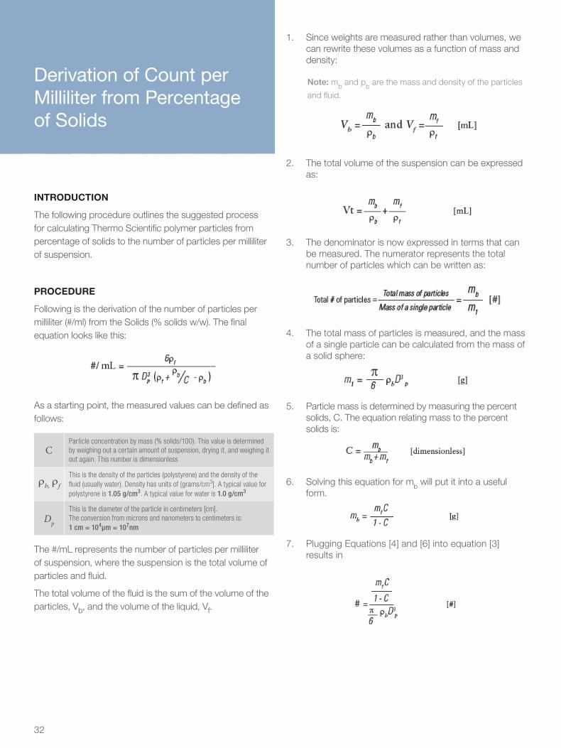
32

Derivation of Count per Milliliter from Percentage of Solids

INTRODUCTION

The following procedure outlines the suggested process for calculating Thermo Scientific polymer particles from percentage of solids to the number of particles per milliliter of suspension.

PROCEDURE

Following is the derivation of the number of particles per milliliter (#/ml) from the Solids (% solids w/w). The final equation looks like this:

As a starting point, the measured values can be defined as follows:

CParticle concentration by mass (% solids/100). This value is determined by weighing out a certain amount of suspension, drying it, and weighing it out again. This number is dimensionless

ρb, ρf

This is the density of the particles (polystyrene) and the density of the fluid (usually water). Density has units of [grams/cm3]. A typical value for polystyrene is 1.05 g/cm3. A typical value for water is 1.0 g/cm3

Dp

This is the diameter of the particle in centimeters [cm]. The conversion from microns and nanometers to centimeters is: 1 cm = 104μm = 107nm

The #/mL represents the number of particles per milliliter of suspension, where the suspension is the total volume of particles and fluid.

The total volume of the fluid is the sum of the volume of the particles, Vb, and the volume of the liquid, Vf.

1. Since weights are measured rather than volumes, we can rewrite these volumes as a function of mass and density:

Note: mb and pb are the mass and density of the particles

and fluid.

2. The total volume of the suspension can be expressed as:

3. The denominator is now expressed in terms that can be measured. The numerator represents the total number of particles which can be written as:

4. The total mass of particles is measured, and the mass of a single particle can be calculated from the mass of a solid sphere:

5. Particle mass is determined by measuring the percent solids, C. The equation relating mass to the percent solids is:

6. Solving this equation for mb will put it into a useful form.

7. Plugging Equations [4] and [6] into equation [3] results in

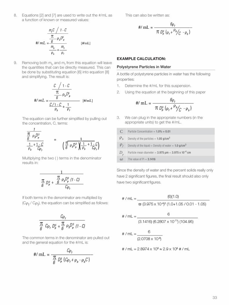
33

8. Equations [2] and [7] are used to write out the #/mL as a function of known or measured values:

9. Removing both mb and mf from this equation will leave the quantities that can be directly measured. This can be done by substituting equation [6] into equation [8] and simplifying. The result is:

The equation can be further simplified by pulling out the concentration, C, terms:

Multiplying the two ( ) terms in the denominator results in:

If both terms in the denominator are multiplied by (Cρf / Cρf), the equation can be simplified as follows:

The common terms in the denominator are pulled out and the general equation for the #/mL is:

This can also be written as:

EXAMPLE CALCULATION:

Polystyrene Particles in Water

A bottle of polystyrene particles in water has the following properties:

1. Determine the #/mL for this suspension.

2. Using the equation at the beginning of this paper

3. We can plug in the appropriate numbers (in the appropriate units) to get the #/mL.

C Particle Concentration = 1.0% = 0.01

ρb Density of the particles = 1.05 g/cm3

ρf Density of the liquid = Density of water ≈ 1.0 g/cm3

Dp Particle mean diameter = 3.975 µm = 3.975 x 10-4 cm

ω The value of Pi = 3.1416

Since the density of water and the percent solids really only

have 2 significant figures, the final result should also only

have two significant figures.

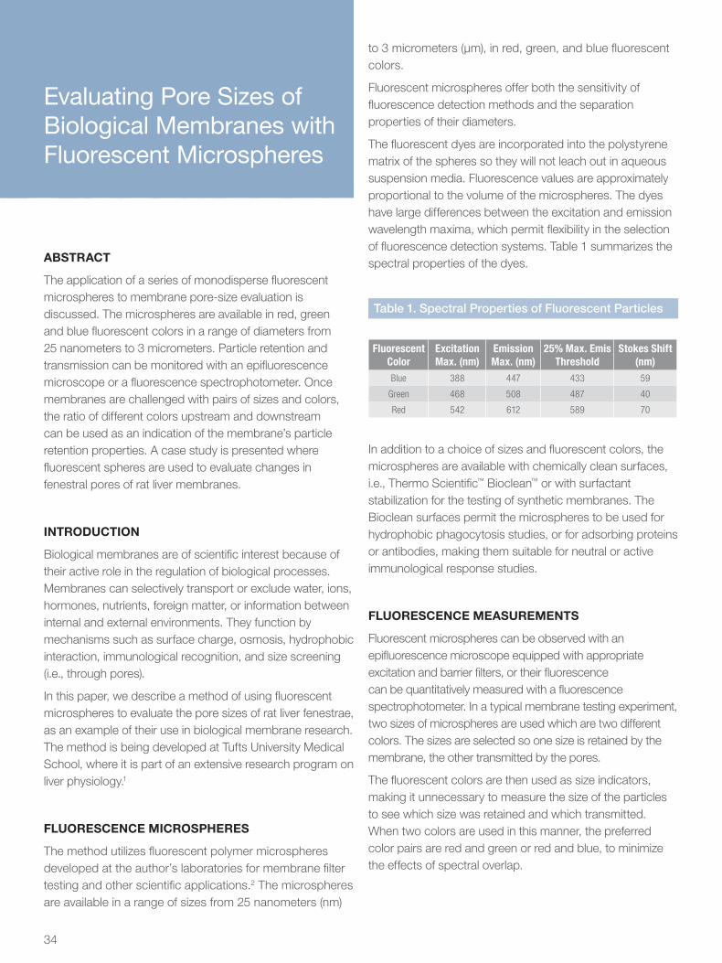
34

Evaluating Pore Sizes of Biological Membranes with Fluorescent Microspheres

ABSTRACT

The application of a series of monodisperse fluorescent microspheres to membrane pore-size evaluation is discussed. The microspheres are available in red, green and blue fluorescent colors in a range of diameters from 25 nanometers to 3 micrometers. Particle retention and transmission can be monitored with an epifluorescence microscope or a fluorescence spectrophotometer. Once membranes are challenged with pairs of sizes and colors, the ratio of different colors upstream and downstream can be used as an indication of the membrane’s particle retention properties. A case study is presented where fluorescent spheres are used to evaluate changes in fenestral pores of rat liver membranes.

INTRODUCTION

Biological membranes are of scientific interest because of their active role in the regulation of biological processes. Membranes can selectively transport or exclude water, ions, hormones, nutrients, foreign matter, or information between internal and external environments. They function by mechanisms such as surface charge, osmosis, hydrophobic interaction, immunological recognition, and size screening (i.e., through pores).

In this paper, we describe a method of using fluorescent microspheres to evaluate the pore sizes of rat liver fenestrae, as an example of their use in biological membrane research. The method is being developed at Tufts University Medical School, where it is part of an extensive research program on liver physiology.1

FLUORESCENCE MICROSPHERES

The method utilizes fluorescent polymer microspheres developed at the author’s laboratories for membrane filter testing and other scientific applications.2 The microspheres are available in a range of sizes from 25 nanometers (nm)

to 3 micrometers (µm), in red, green, and blue fluorescent colors.

Fluorescent microspheres offer both the sensitivity of fluorescence detection methods and the separation properties of their diameters.

The fluorescent dyes are incorporated into the polystyrene matrix of the spheres so they will not leach out in aqueous suspension media. Fluorescence values are approximately proportional to the volume of the microspheres. The dyes have large differences between the excitation and emission wavelength maxima, which permit flexibility in the selection of fluorescence detection systems. Table 1 summarizes the spectral properties of the dyes.

Table 1. Spectral Properties of Fluorescent Particles

Fluorescent Color

Excitation Max. (nm)

Emission Max. (nm)

25% Max. Emis Threshold

Stokes Shift (nm)

Blue 388 447 433 59

Green 468 508 487 40

Red 542 612 589 70

In addition to a choice of sizes and fluorescent colors, the microspheres are available with chemically clean surfaces, i.e., Thermo Scientific™ Bioclean™ or with surfactant stabilization for the testing of synthetic membranes. The Bioclean surfaces permit the microspheres to be used for hydrophobic phagocytosis studies, or for adsorbing proteins or antibodies, making them suitable for neutral or active immunological response studies.

FLUORESCENCE MEASUREMENTS

Fluorescent microspheres can be observed with an epifluorescence microscope equipped with appropriate excitation and barrier filters, or their fluorescence can be quantitatively measured with a fluorescence spectrophotometer. In a typical membrane testing experiment, two sizes of microspheres are used which are two different colors. The sizes are selected so one size is retained by the membrane, the other transmitted by the pores.

The fluorescent colors are then used as size indicators, making it unnecessary to measure the size of the particles to see which size was retained and which transmitted. When two colors are used in this manner, the preferred color pairs are red and green or red and blue, to minimize the effects of spectral overlap.

35

Microspheres 180 nm or larger in diameter can be seen with a properly equipped fluorescence microscope. Those smaller than 180 nm are easily measured with a spectrophotometer. Larger microspheres may also be measured with a spectrophotometer, subject to light- scattering limitations. When absolute fluorescence values are required for maximum accuracy, a solvent such as methyl pyrollidone can be used to dissolve the polymer matrix and make a clear solution of the dye for direct fluorescence measurements.

RAT LIVER STUDIES

Fluorescent microspheres can be observed with an epifluorescence microscope equipped with appropriate excitation and barrier filters, or their fluorescence can be quantitatively measured with a fluorescence spectrophotometer. In a typical membrane testing experiment, two sizes of microspheres are used which are two different colors. The sizes are selected so one size is retained by the membrane, the other transmitted by the pores.

Figure 1. Rat Liver Fenestrae (bar ~ 1μm)

Investigations of rat liver fenestrae (openings, or pores) were conducted at Tufts University Medical School to determine their changes in diameter as a function of stimulating factors in the bloodstream. The fenestrae are located in the endothelial cells of liver capillaries. Illustrated in Figure 1, they have a normal diameter of approximately 100 nm and act as a biological “screen” along the lumen of the capillary3.

They are a transport medium between the hepatic cells of the liver and the flow channel of the capillary. The pores are believed to contract or dilate over a range of 80 to 120 nm under certain conditions, which are being studied with this method.

In addition to the endothelial cells containing the fenestrae, the capillary has macrophages known as Kupffer cells located at intervals inside the membrane. The Kupffer cells play an immunological role in the membrane; they phagocytose large foreign particles. The two kinds of cells combine their functions to capture or delay the passage of particulate matter through the capillaries. Using fluorescent microspheres in various sizes, colors, and surface treatments, both the size changes and the screening mechanisms of the fenestral pores can be studied.

PERFUSION SYSTEM

A pump and temperature controlled reservoir are used to perfuse Krebs-Ringer buffer through the rat liver in-vivo. The stream enters the portal vein and exits from the vena cava, where it is collected as a series of fractions for further analysis. A precision syringe is used to inject a bolus of microspheres into the perfusion stream for the test. The rat liver is maintained by continuously adjusting the perfusion medium to a pH of 7.4 with NaOH or HCl, and monitoring its oxygen uptake as an indication of its viability.

Fluorescence spectra for the microspheres was measured on a PerkinElmer™ Model LS-5 Spectrometer 4. They are typically measured at fixed wavelengths of both excitation and emission, which provides an index of microsphere perfusion through the system. The fluorescence spectra are used to distinguish between particle sizes in the eluted fractions. Since the two sizes of particles take different amounts of time to perfuse through the liver, the fluorescence spectra of each fraction permits an elution profile to be plotted for each microsphere size.

EXPERIMENTAL PROCEDURE

The perfusion buffer and solutions consist of 2 liters of Krebs-Ringer (bicarbonate) at pH 7.4; 100 mL of physiologically buffered saline (PBS) at pH 7.2; and a solution of bovine serum albumin (BSA) for coating the microspheres (4% in PBS). After sonicating the microspheres for 30 to 60 seconds to assure their dispersion, a 1.6 mL suspension of coated microspheres is prepared by combining 0.800 mL of BSA solution, 0.560 mL of PBS solution, and 0.240 mL of microspheres (1% solids). This 1.6 mL combination is allowed to incubate for 2 hours at room temperature so the BSA molecules can adsorb onto the microsphere surfaces. The 0.240 mL of microsphere suspension should include the two different colors and sizes of the microspheres at the desired ratios.

36

The baseline fluorescence values are obtained by taking a 0.2 mL aliquot of the 1.6 mL microsphere suspension, diluting it in 6ml of perfusion buffer, measuring the fluorescence of the two dyes, and multiplying the fluorescence values by 30 and by 0.2 mL (or the exact weight of the sample in grams). These are the total uninjected fluorescence values per unit volume.

The perfusion system is set up with the rat liver in place and the perfusion flow rate set at 30 mL per minute. After the viability of the rat liver is verified by observing the oxygen uptake rate, another 0.2 mL aliquot of the microsphere suspension is injected into the perfusion stream. The fraction collector is adjusted to collect 50 fractions in one minute, approximately 0.64 mL each. The fluorescence values for each color are measured for each fraction and compared to the standard fluorescence curve to obtain the ratio of recovered spheres to injected spheres at each time interval. In most cases, the first 25 fractions contain sufficient fluorescence for one set of data. The 1.6 mL of microsphere suspension is usually enough for four or five experiments including the fluorescence baseline calibration.

RESULTS AND CONCLUSIONS

As expected, the larger particles were generally eluted before the smaller particles, which were delayed by their tortuous path through the fenestrae.

However, higher percentages of the smaller particles were typically recovered, probably because many of the larger particles were retained by the phagocytic action of the Kupffer cells.

The BSA coated microspheres were recovered at a much higher rate than the uncoated microspheres, due to the interaction between the various protein surfaces along the membrane and the hydrophobic surface of the uncoated polystyrene microspheres.

No significant difference was found between microspheres coated with rat serum albumin and BSA.

Table 2 summarizes the recovery values for a series of coated and uncoated microspheres, in various sizes and fluorescent colors.

Table 2. Recovery Rates of Fluorescent Microspheres

MicrosphereDiameter (nm)

ColorBovine Serum

UncoatedAlbumin Coated

47 Red 69.7

76 Green 13.7

86 Green 75.5

105 Red 13.2

111 Green 57.6

150 Blue 15.6

185 Green 18.6 55.3

204 Red 46.8

210 Green 18.8

312 Red 22.5 51.4

532 Red 21.3 38.5

Additional procedures are being studied to refine the method, but it has been proven to be effective and useful by the Tufts University group. Changes in fenestral pore diameters as a function of stimulating agents in the bloodstream can now be studied in detail, meeting the original goals of the program.

SUMMARY

Evaluation of rat liver fenestrae is only one example of the many potential applications of fluorescent microspheres to the field of membrane studies. The microspheres can be used to study a variety of screening and capture mechanisms, and can be adapted to the study of membrane immunological properties.

REFERENCES

1. Method developed by I. M. Arias, Z. Gatnaitan, and K. Akamatsu, Dept. of Physiology, Tufts University School of Medicine, 136 Harrison Avenue, Boston, MA 02111. http:europepmc.org/backend/ptpmcrender.fcgi?accid=PMC1861643&blobtype=pdf

2. S. D. Duke, “Particle Retention Testing of 0.05 to 0.5 Micrometer Membrane Filters”, Proceedings, International Technical Conference on Filtration and Separation, p. 523- 532, (1988), American Filtration Society, P.O. Box 6269, Kingswood, TX 77325.

3. Kirn, A., Ed., D.L. Knook and E. Wisse, Cells of the Hepatic Sinusoid, Vol. 1 (1986).

4. The Perkin-Elmer Corporation, Norwalk, CT 06856

5. The BIOCLEAN™ product line is no longer available for retail sale. Many alternative products for this type of testing are available.

QC / CALIBRATIONTECHNICAL NOTES ON

38

The Importance of Measurement Components in Instrument Calibration and Method Validation

INTRODUCTION

This technical note describes the components of measurement for Thermo Scientific NIST (National Institute of Standards and Technology) traceable particle size standards. These are listed on the labels of these products as follows:

• Mean diameter

• Uncertainty

• Standard deviation

• Coefficient of variation

This information is representative of a complete characterization of a calibration standard.

By employing detailed measurement methods that utilize optimized measurement scales and standards with a high number of significant figures, Thermo Scientific size standards are designed to enable users to achieve better and greater consistency in the calibration of their measurement systems.

MEAN DIAMETER AND UNCERTAINTY

The mean diameter reported by Thermo Fisher Scientific is the arithmetic mean size of the particles, which is measured using methods that provide traceability to NIST Standard Reference Materials. The mean diameter is expressed here:

Y μm ± U μm

Y is the mean diameter and U is the uncertainty associated with the measurement of the mean diameter.

The uncertainty U is specific to the mean diameter measurement method and does not convey any information about the size distribution.

The proper representation and importance of measurement uncertainty is detailed in NIST Tech Note 1297, Guidelines for Evaluating and Expressing the Uncertainty of NIST Measurement Results, and in the ISO IEC Guide 98-3:2008 Uncertainty of Measurement.

The uncertainty is calculated from the observed variation in individual measurements taken (Random or Type A values) and possible sources of error in the system (Systematic or Type B values).

We provide an expanded uncertainty for a 95% confidence level of the actual mean diameter. The value of providing the mean diameter and expanded uncertainty is that users get measurements that allows them to calibrate their instruments and validate their methods using NIST traceable standards.

For more information on how the expanded uncertainty is calculated, refer to NIST Technical Note 1297.

THE IMPORTANCE OF UNCERTAINTY

According to NIST Technical Note 1297, a measurement result is complete only when accompanied by a quantitative statement of its uncertainty. This measurement of uncertainty is important because it defines with a stated degree of confidence the range of values within which the actual mean diameter will reside.

Without having knowledge of the mean diameter measurement uncertainty, one risks basing their application or methods on potentially erroneous information.

REPRESENTATION OF UNCERTAINTY

To further show how the measurement uncertainty is reported, consider the Thermo Scientific 4205A nominal 5.0 μm particle size standard which has a mean diameter of 5.003 μm with an expanded uncertainty of ± 0.043 μm. This signifies that the mean diameter has a 95% probability of being between 4.960 μm and 5.046 μm.

In comparison, the Thermo Scientific 2005A nominal 5 μm particle size standard has a mean diameter of 5.0 µm ± 0.3 µm. In this case, the mean diameter has a 95% probability of being between 4.7 and 5.3 μm.

STANDARD DEVIATION AND COEFFICIENT OF VARIATION

While the expanded uncertainty describes the actual measurement, the standard deviation (σ) and coefficient of variation (CV) describes the particle population size distribution.

39

Knowing the particle size distribution is vital for most applications, but especially for instrument calibration.

The CV is the standard deviation divided by the mean expressed as a percentage. In other words, it is one standard deviation as a percent of the mean diameter. The CV allows one to compare the extent of size distributions for different particle products and particle lots of the same diameter. A CV of less than 3% indicates a population that has a narrow distribution about the mean diameter, whereas as a CV of greater than 3% indicates a wider distribution.

This graph illustrates the comparison between the Thermo Scientific 4205A and 2005A NIST traceable size standards, both with a nominal diameter of 5 µm.

While the 2005A product (blue line) has a normal Gaussian distribution of particles with a CV greater than 5%, the 4205A product (purple line) has a very narrow distribution with a CV < 3%.

Knowing the size distribution of standards is useful as it allows the customer to select a standard with a distribution appropriate to the resolution of their instruments.

CONCLUSION

A complete characterization of a calibration size standard includes a mean diameter, the uncertainty of the mean diameter, a standard deviation, and the coefficient of variation.

Furthermore, a well characterized particle size standard provides a higher level of confidence in the mean diameter. Having this confidence is important for instrument calibration and validation. Every measurement, no matter how precise, will carry some degree of uncertainty.

Knowing with confidence the mean diameter, uncertainty, standard deviation and CV of your calibration standard (which Thermo Scientific provides) will lead to better calibrations and validations.

REFERENCES

1. Bell S.; A beginners guide to Uncertainty in Measurement, NPL. Issue 2, 1999.

2. Taylor, B.N.; Kuyatt, Chris E; NIST Tech Note 1297; September 1994

3. ISO IEC Guide 98-3:2008 Uncertainty of Measurement.

40

Improved Array Method for Size Calibration of Monodisperse Spherical Particles by Optical Microscope

ABSTRACT

Monodisperse or highly uniform spheres, when placed on a flat surface in a liquid medium, align themselves into systematic hexagonal arrays characterized by straight rows of particles. Using an optical microscope, the length of a row can be measured and divided by the number of spheres in the row to calculate the average diameter of the spheres. Limitations of the traditional array methods have been avoided by improved sample preparation methods and careful selection of measurement rows.

Using the improved method, a series of monodisperse spherical particles from 0.5 to 40 micrometers (μm) were calibrated and certified with a stage micrometer calibrated by the National Institute of Standards and Technology (NIST).

INTRODUCTION

When placed on a flat surface in a liquid medium, monodisperse or highly uniform spheres align themselves into systematic hexagonal arrays characterized by straight rows of particles. Using a calibrated optical microscope, the length of a row can be measured, then divided by the number of spheres in the row to calculate the average diameter of the spheres.

Array methods for determining the mean diameter of spherical particles have been in use since 1977. The methods were developed because of the difficulty of determining the edge of spherical particle images with high precision as shown in (Figure 1). When the spheres are in contact in a straight line on a flat surface, the uncertainty of defining the outside edge of the first and last particle in an array is the same as for both edges of a single particle. When the uncertainty is divided by the number of spheres in the row, the edge uncertainty per sphere becomes very low, greatly improving the accuracy of the mean size determination. Figure 2 shows a typical array.

Other laboratories have also used array methods successfully.1 Kubitschek2 and Hartman3,4 have described errors in previous methods which can be overcome with the techniques we have developed.

When the mean diameter of monodisperse particles is of primary importance, rather than the size distribution, the array method is a convenient and practical method. This report describes our method and gives the results of the measurement of selected reference standards from 0.46 to 40 μm.

Figure 1. Typical edge images for 9.87 µm spheres, 8 µm per division.

Figure 2. 9.87 µm spheres in arrays, 4 µm per division.

EQUIPMENT AND METHODS

The microscope used in this work is an Olympus™ BHA. It has a 15x magnifying eyepiece and is equipped with an eyepiece reticle and objectives of 10, 20, 40, 60 and 100x magnifications.

41

Stage Micrometer - Primary Standard

The primary calibration standard is a stage micrometer calibrated for 31 intervals by laser interferometry by the National Institute of Standards and Technology (NIST)5. The uncertainty of the micrometer calibration, from NIST Report #5524, is less than 0.00004 mm (0.04 µm) for lengths less than 0.2 mm, the longest length used to calibrate the eyepiece reticle.

The micrometer was calibrated at 20°C and has a thermal coefficient of expansion of 8.5 parts per million per °C. The maximum error due to thermal expansion is 0.004%. The micrometer is 2 mm in length divided in 200 divisions, with line widths of 2 µm, and sharp line edges as shown in Figure 3.

Verification Standards

Our own in-house size standards and several certified particle size standards from NIST and from the Community Bureau of Reference (BCR)6 were used as verification standards. They were measured for spherical diameter using the improved array method. The three BCR Standard Reference Materials analyzed are BCR #165A (2.223 µm), BCR #166A (4.821 µm), and BCR #167A (9.475 µm), calibrated by the optical array method. The three NIST Reference Materials are SRM #1690 (0.895 µm), SRM #1960 (9.89 µm) and SRM #1961 (29.64 μm).7 The eight Nanosphere size standards were calibrated by transmission electron microscopy (TEM) using the internal standard method8,9 with SRM #1690 (0.895 μm) as the reference standard.

Calibration

The microscope eyepiece reticle was calibrated by measuring intervals on the NIST-calibrated stage micrometer with the eyepiece reticle (Figure 4). It is critical that the eyepiece reticle be well focused for the microscope operator, and that the eyepieces of binocular microscopes are carefully focused to the operator’s eyes. To minimize the effect of spherical aberration, only the central 20% of the eyepiece reticle, which has no apparent distortion, was calibrated. No lengths were measured at more than 25 divisions (<20% of the field), as beyond this point, the field is not optically flat. In general, the reticle should be calibrated as close as possible to the length of the array being measured.

Array Preparation

There are several methods of preparing measurable arrays, but the general method involves inducing the spheres to array in monolayers by drawing the microsphere suspension between microscope slide and cover-glass by capillary action. Anything that disturbs this smooth flow will interrupt array formation.

Figure 3. The NIST-calibrated stage micrometer, 10 µm per division.

by Optical Microscope (Continued)

Figure 4. The stage micrometer through the eyepiece reticle, 8 µm per reticle division.

If the array formation is too slow, the microspheres will array loosely, making them appear larger than they actually are. This can be detected by measuring the array in two different directions; if there is any variation, the section of arrays in question should not be used.

If the microspheres array too fast, they will pack too tightly, and not all of them will be in contact with the slide. This produces arrays that appear striated when slightly defocused, and will show an average diameter smaller than the actual diameter.

The greatest problems in producing measurable arrays are flocculation, or the presence of clumped particles or large spheres. These can cause the microspheres to array in multilayers. Near-size large and small particles can make holes or gaps in the arrays, causing the rows to crack or bend. Preparation of good, measurable arrays requires microsphere suspensions that contain a minimum of large or small outliers or clumps of particles, and have proper dispersing agents to prevent flocculation during array formation.

42

Row Selection

Rows were selected that were in flat monolayer arrays, without large or small particles, cracks or gaps. They were perfectly straight when compared to the eyepiece reticle, and were at least 10 divisions long whenever possible. Row lengths were measured on the eyepiece reticle by placing a reticle line exactly between two beads and counting the number of beads until the edge of a bead corresponds closely with another line. The length (to the nearest tenth of a division) and the number of spheres in the row were recorded. At least 9 rows were measured for each sample. The row lengths can be measured directly by the microscope operator or photographed for later analysis.

These values were entered in a double precision computer program created specifically for the array method which automatically adjusts for the scale calibrations. The mean is calculated as the sum of the row lengths in micrometers divided by the total number of spheres measured. Figure 5 shows a typical row with the eyepiece reticle in place.

Figure 5. 9.87 µm arrayed spheres through the eyepiece reticle, 4 µm per division.

Analysis of Uncertainty

The total uncertainty is the sum of the random measurement error and the calibration uncertainty (Table 1). The calibration uncertainty was calculated as the sum of the stage micrometer calibration uncertainty (from NIST report #5524) and the estimated uncertainty of determining the edge of the stage micrometer lines by the microscope operator.

To determine the random error of the measurements, the mean diameter of each row measurement was considered as one determination. The precision of the measurements is the standard deviation of the mean diameters for each individual row. Errors in locating the edges of the spheres are included in the row-length variation.

Table 1. Sources of Uncertainty for 10 µm Spheres

Error Source Uncertainty Amount

A. Calibration Uncertainty

1. Uncertainty in the Stage Micrometer 0.05 µm per measurement

2. Location of Micrometer Line Edges (5% of 1.7 µm width x 2)

0.17 µm per measurement

Total Calibration Uncertainty 0.22 µm per measurement

3. Average spheres per measurement 14 spheres

4. Calibration error per sphere (0.22 µm/14 spheres)

0.016 µm per sphere

B. Random Measurement Uncertainty

5. Standard Deviation of measurements 0.040 µm per sphere

C. Total Uncertainty of the Mean Diameter

6. Sum of A-4 and B: 0.056 µm per sphere

Table 2: Comparison of the Array Method with Certified Diameters of Reference Standards

Reference Material

Certified Diameter (µm)

Array Value (nm)Difference

(%)

3450A (TEM) 0.460 ± 0.004 0.458 ± 0.019 -0.002 -0.43

3500A (TEM) 0.496 ± 0.004 0.497 ± 0.023 0.001 0.20

3600A (TEM) 0.597 ± 0.005 0.597 ± 0.017 0 0

3700A (TEM) 0.705 ± 0.006 0.706 ± 0.021 0.001 0.14

3800A (TEM) 0.798 ± 0.007 0.799 ± 0.017 0.001 0.13

NIST SRM 1690 0.895 ± 0.008 0.895 ± 0.008 0 0

4009A (TEM) 0.993 ± 0.021 0.992 ± 0.017 -0.001 -0.10

BCR 165A #3 2.223 ± 0.013 2.224 ± 0.032 0.001 0.04

BCR 166A #4 4.821 ± 0.019 4.821 ± 0.036 0 0

BCR 167A #1 9.475 ± 0.018 9.471 ± 0.062 -0.004 -0.04

NIST SRM 1690 9.89 ± 0.04 9.896 ± 0.066 0.006 0.06

NIST SRM 1690 29.64 ± 0.06 29.58 ± 0.06 -0.06 -0.20

Figure 6. Array Method: Observed vs. Expected Values for Standards.

43

RESULTS

The expected values and the values observed by array method for the certified reference standards are summarized in Table 1. There was no bias observed, meaning that the systematic error was not significant. The average percent differences between the observed and expected values, 0.1 %, can be considered random or measurement error. The measured value was within the uncertainty of the certified value for the standards in all cases. Figure 6 is a graph of the expected vs. observed values of 2005A NIST traceable size standards, both with a nominal diameter of 5 μm.

CONCLUSION

Although limited primarily to the measurement of monodisperse microspheres, the array method offers improved mean size analysis compared to most one- by-one particle sizing methods, provided the arrays are measured by the recommended procedures. It correlates extremely well with more sophisticated and complicated methods for calibrating particle size standards, can be NIST traceable, and is relatively easy to perform. Using the improved array method, a new series of particle size standards from 1.0 to 100 μm have been calibrated and certified which leads to better calibrations and validations.

REFERENCES

1. Thom, R., H. Marchandise and E. Colinet, “The Certification of Monodisperse Latex Spheres in Aqueous Suspensions with Nominal Diameter 2.0µm, 4.8µm and 9.6µm”, Calibration Report EUR 9662 EN, Community Bureau of Reference (1985).

2. Kubitschek, Herbert E., “The Array Method of Sizing Monodisperse Particles”,in Ultrafine Particles, ed. W.E. Kuhn, Wiley, p.438-454, (1963).

3. Hartman, A.W., “Investigations in Array Sizing, Part 1: Accuracy of the Sizing Process”, Powder Technology 39, p. 49-59, (1984).

4. Hartman, A.W., “Investigations in Array Sizing, Part 2: The Kubitschek Effect”, Powder Technology 42, p. 269-272, (1985).

5. National Bureau of Standards Technical News Bulletin, Vol. 51, #3, March 1967. Now the National Institute of Standards and Technology.

6. Community Bureau of Reference, Commission of the European Communities, 200 rue de la Loi, B-1049, Brussels, Belgium.

7. National Intitute of Standards and Technology, U.S. Department of Commerce, Gaithersburg, Maryland, 20899.

8. Mulholland, G.W., A.W. Hartman, G.G. Hembree, Egon Marx, and T.R. Lettieri, “Development of a One-Micrometer- Diameter Particle Size Standard Reference Material”, Journal of the National Bureau of Standards 90, p.3-26, (1985).

9. Duke, S.D., and E.B. Layendecker, “Internal Standard Method for Size Calibration of Sub-Micrometer Spherical Particles by Electron Microscope”, Proceedings of the Fine Particle Society, (1988).

10. The original publication of this paper pre-dates NIST Technical Note #1297, therefore the uncertainty calculation follows the guidelines in place at the time instead of the TN1297 / ISO GUM methods.

44

Calibration of Spherical Particles by Light Scattering

ABSTRACT

Photon Correlation Spectroscopy, also known as Quasi-Elastic or Dynamic Light-Scattering, can be a convenient method of size measurement for suspensions of monodisperse spherical particles in the 20-500 nanometer (nm) size range [0.02 to 0.5 micrometer (µm)]. The results obtained vary widely, depending on the concentration and condition of the sample, as well as environmental factors. Techniques have been developed that improve the accuracy and precision of the measurements. These techniques include controlling the concentration, uniformity and dispersion of the sample. The improved method was verified by measuring particle size standards.

INTRODUCTION

Photon Correlation Spectroscopy (PCS) and Quasi- Elastic Light Scattering (QELS) are promising methods for the measurement of suspended particles from 20- 500nm. In principle, these instruments do not require calibration, since they calculate the mean diameter of the particles by observing fluctuations of scattered light related to the diffusion coefficient of the sample. In a medium of known viscosity, temperature, and refractive index, the diffusion coefficient is directly related to the Brownian motion of the particles. In practice, the commercially available instruments, although relatively easy to operate, do not provide the kind of accuracy and precision required by our laboratory. In order to meet our objectives, we developed a series of procedures for preparing samples and optimizing their analysis to overcome the limitations of the instruments.

This report describes our methods for the benefit of those who want to optimize the performance of their PCS/ QELS instruments for the measurement of polystyrene latex microspheres.

There are four principal considerations that have proven to be of crucial importance for obtaining accurate size results from the PCS instruments: i) electrolytic activity in the analysis

diluent; ii) particle concentration of the sample; iii) temperature conformity between the sample and the set temperature of the instrument; and iv) sample dispersion and uniformity.

ELECTROLYTIC ACTIVITY OF DILUENT

Suppliers of PCS instruments sometimes recommend using ultrapure water for the diluent. Most “ultrapure” water systems deliver water filtered to 0.2 μm or smaller and 18 micro ohm resistance. The problem with such water is that it does nothing to contribute to the dispersion stability of typical polystyrene latex microspheres, whose stabilization depends on the effect of negatively charged sulfate groups on the particle surface.

When there is a lack of effective conductance of the surface charges, a temporary hydrophobic interaction between the particles results. The associated particles will exhibit reduced Brownian motion and a larger diameter for the duration of the interaction. Thus, the PCS instrument will measure a larger particle diameter and usually, a higher polydispersity factor. For the sulfate groups to exhibit a sufficient repulsive force, a certain measure of electrolyte is needed to conduct the surface charges.

The electrolyte selected by our laboratory for all PCS measurements of polystyrene latex is a 1000 micro ohm conductivity solution of tetrasodium pyrophosphate (TSPP), approximately 0.16 wt%. This amount does not appreciably alter solution density or viscosity from that of pure water. The procedure is used exclusively for conventional polystyrene latex and does not apply to carboxylated and other surface-modified particles.

The optimum electrolyte should be somewhat basic in order to completely ionize the sulfate groups on the surface of the particles. It is also desirable for the electrolyte to function as an ionic dispersant, supplementing the polystyrene surface charges. In addition, the electrolyte must be used at a concentration that offers the best possible zeta potential for inhibiting the interaction of the particles.

The TSPP diluent is basic, approximately pH 10 at the 1000 micro ohm conductivity is recommended for the electrolyte. It is also only slightly water soluble, meaning that the TSPP molecules will have a certain affinity for the surface of the particles. Unlike a surfactant where a hydrophobic end is attracted to a particle surface, such dispersion stabilization occurs through simple solubility considerations.

The ionic species are simply concentrated near the particle surfaces and add additional surface charges, meaning both pyrophosphate and sulfate groups aid in preventing association of particles in solution.

45

As with any PCS measurement, the diluent must be free of foreign particulates. It is thus best to filter this electrolyte solution using at least 0.2 µm filtration, while minimizing contaminants from the filter media.

As shown in Table 1, when clean 1000 micro ohm TSPP electrolyte was used as a diluent to analyze Thermo Scientific Nanosphere polystyrene size standards, the observed diameter was always smaller than for the same spheres in deionized water. As is shown later, the smaller diameter is usually the correct diameter. The instrument used was a Brookhaven™ BI-90 with a 633nm laser. The temperature was approximately 20-23°C and viscosity was set for the temperature.

Table 1. Effect of Suspension Media on PCS/QELS Values

Catalog PN TestedPCS Diameter with

TSPP (nm)PCS Diameter with

ultrapure water (nm)3050 52.7 57

3060 62.8 69

3100 108 112

3150 155 166

3200 219 237

3269 270 285

3300 299 316

PARTICLE CONCENTRATION ADJUSTMENTS

The optical system of a PCS instrument can be constructed in various ways, and we have found a considerable difference in the optimum particle concentration required for instruments from different manufacturers. Some instruments, especially modern ones with more powerful lasers, require a more dilute sample concentration than, for example, the Brookhaven BI-90.

Our laboratory achieved the greatest success in optimizing sample concentrations by measuring their turbidity on a spectrophotometer at the 633nm wavelength. This technique measures the turbidity of the sample, allowing us to adjust it at the PCS laser wavelength.

As shown in Table 2, when measuring the National Institute of Standards and Technology (NIST) 269 nm standard (SRM 1691)5, with TSPP 1000 micro ohm electrolyte, both the diameter and polydispersity values changed as a function of concentration on a Brookhaven BI-90 analyzer.

Table 2. Effects of Sample Concentration on PCS/QELS Values

Absorbance@ 633 nm

Count Rate (Kcps)

Diameter (nm) Polydipersity Index

0.020 142 272.5 0.040

0.036 221 271.8 0.036

0.076 458 270.1 0.043

0.101 537 268.4 0.062

0.145 648 267.2 0.066

For analyses below about 300 nm, the BI-90 instrument yielded the best data at or near 0.045 absorbance. For sizes above 300 nm, it is necessary to increase the turbidity in successive amounts. Approximately 0.20-0.25 absorbance is optimal for the 0.5 μm size.

It is desirable to establish a concentration curve, which is generated using a range of appropriate standards in an electrolyte diluent. For each particle diameter there would then be an optimum absorbance value and particle concentration (KPCS) for obtaining the most accurate size.

We have since developed another method to determine the optimum concentration and use it for the preparation of all samples.

TEMPERATURE CONTROL

Since the diameter obtained by PCS is inversely proportional to sample viscosity, it is essential that the sample temperature matches the set point of the instrument sample holder. At our lab, we measure the temperature before inserting it into the instrument and again immediately after the runs are completed. Often adjustments are needed in the diameter value because the average temperature over the course of the runs does not equal the set point.

These adjustments have ranged to as high as ±3% of the diameter value, and cannot be dismissed as insignificant when attempting to obtain the most accurate size data possible. Figure 1 shows the range of error that can be expected for discrepancies between true and set point temperatures.

46

Figure 1. PCS/QELS Sensitivity to Temperature Variation

SELECTING AND PREPARING SAMPLES

Many materials used as PCS reference particles are not supplied in a dispersion of suitable quality to yield accurate size data. Frequently, polystyrene latex batches sold directly from the reactor contain a considerable amount of debris, and are at high solids concentrations.

Some of these materials are relatively old and, in the course of aging, have formed hard aggregates which can not be dispersed by sonication or surfactants. Many of the difficulties encountered with the data from PCS instruments can be traced to poor quality of the initial particle dispersion.

In some instances, a polystyrene latex suspension may contain an abundance of off-size small and large particles, which can skew a PCS analysis. More typically, the number of such undesirable particles is small and the impact upon analysis may be more subtle.

The greatest problem is with near-oversized particles and with aggregates of the main population, since PCS systems are most sensitive to these particles. In the case of very small particles, it may be useful to use a 0.1, 0.2, 0.45, or 1.0 µm filter to remove oversized particles and debris from the diluted sample.

Unless steps are taken to remove undesirable particulates and debris from bulk polystyrene latex samples, they can reduce the accuracy and reproducibility of PCS evaluations. A summary of these adverse effects is shown in Table 3.

Table 3. Effects of Off-size Particulates and Dispersion Quality on PCS/QELS Size Measurements

Problem Effect

Debris from latex reactor Oversizes and broadens the distribution

Undispersed clumps of particles Oversizes and broadens the distribution

Near-sized large particles Oversizes and broadens the distribution

Near-sized small particles Undersizes and broadens the distribution

Ultrafine particles Negligible, depending on quantity

RESULTS AND CONCLUSIONS

The procedures employed here will reduce the artifacts induced by factors such as dispersion, concentration, temperature, and sample anomalies in PCS measurements. Our laboratory has found very good agreement between PCS and accurate transmission electron microscopy (TEM) measurements, but only when these conditions are optimized (see Table 4 and Figure 2).

The TEM number-weighted values were adjusted to the intensity-weighted values typically measured by PCS instruments. Since the instruments vary in performance by make and model, these optimized measurements will permit more effective evaluation and use of the instruments.

The Thermo Scientific Nanosphere line of size standards have been developed using the described optimized methods.

Table 4. Optimized PCS/QELS Values vs. Reference Standards data

Catalog PN Tested

TEMDiameter (nm)

TEM Intensity Weighted (nm)

PCS/QELSDiameter (nm)

3050A 50.5 52.1 52.7

3060A 63.7 62.9 62.8

3070A 73.1 74.3 74.0

3080A 81.4 83.0 82.9

3090A 96.0 97.9 97.0

3100A 107 107 108

3125A 126 126 126

3150A 155 155 155

3220A 220 220 219

3269A 269 269 270

3300A 298 298 299

3350A 343 343 344

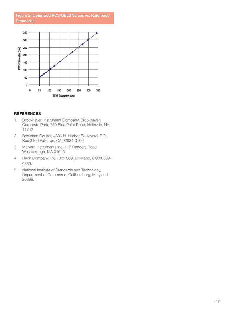
47

Figure 2. Optimized PCS/QELS Values vs. Reference Standards

REFERENCES

1. Brookhaven Instrument Company, Brookhaven Corporate Park, 750 Blue Point Road, Holtsville, NY, 11742

2. Beckman Coulter, 4300 N. Harbor Boulevard, P.O. Box 3100 Fullerton, CA 92834-3100.

3. Malvern Instruments Inc. 117 Flanders Road Westborough, MA 01545.

4. Hach Company, P.O. Box 389, Loveland, CO 80539-0389.

5. National Institute of Standards and Technology, Department of Commerce, Gaithersburg, Maryland, 20899.

48

Internal Standard Method for Size Calibration of Sub-Micrometer Spherical Particles by Electron Microscope

INTRODUCTION

Transmission Electron Microscopy (TEM) is an accepted method for measuring the mean diameter and size distribution of polymer latex microspheres1,2. However, errors in the size data of uniform latex particles from commercial suppliers3, and the need for traceability of size data to the National Bureau of Standards (NBS)4, raise doubts about the suitability of TEM size data for calibrating spherical size standards. In addition to needing accurate data, the authors’3 laboratory needed to calibrate smaller than usual latex microspheres. By omitting several sources of error in typical TEM calibration procedures5,6 and by modifying the sample preparation procedure, we were able to make improvements in the method. This enabled us to calibrate a new series of polymer microspheres for use as certified particle size standards from 50 nanometers (nm) to 1 micrometer (μm).

TEM CALIBRATION PROBLEMS

Most of the methods of calibrating TEM’s have problems, which contribute to the uncertainty of the measurements. The most common method is to use magnification directly to determine the size of the particles. A slight variation of this method is to photograph a grating replica to calibrate the magnification of the photomicrograph, which is then used to measure the diameter of the particles. The problem with these two procedures is that, in the authors’3 experience, the differences between stated and measured magnifications can be as much as 5%. The actual magnification can also vary as much as 2% between consecutive photos at the same magnification on the same instrument. In addition, the apparent distortion of polymer microspheres under the electron beam2,3,6 contributes to measurement errors, along with the possibility of photographic prints stretching or shrinking during the drying process.

Another method is to mount the spheres on a diffraction grating replica and use the grating to provide the scale. The main problem with this method is the lack of certainty regarding the actual line spacing of the replica. Commercially available replicas are not certified for line spacing accuracy or traceability to NBS. While the 463 nm line spacing scale is adequate for larger diameter spheres, it is not suitable for spheres smaller than 200 nm. At such magnification the edge of the grating line is almost as wide as the particle being measured, and if the surface of the replica is rough, the coarseness bleeds through the image, making the sphere edges difficult to locate (Figure 1).

Figure 1. 100 nm latex microspheres on a 2160 line/mm grating

INTERNAL STANDARD METHOD

To reduce the error involved with grating replicas or other calibration methods, the spheres being analyzed are mixed with either NBS Standard Reference Materials 1691 (0.269 µm), 1690 (0.895 µm)7,8, or Thermo Scientific Nanosphere Size Standards to provide an internal calibration reference. Thus, the exact magnification can be determined for each photograph from the known diameter of the standard microspheres. For the measurement of monodisperse spheres, the calibration spheres need only be about 10% to 20% larger or smaller than the particles to be measured. For samples with a size distribution, the diameter of the calibration spheres should be outside the size range of the sample to avoid overlapping diameters.

When used to calibrate polystyrene spheres, this method eliminates errors due to distortion of the spheres by the electron beam. Because the calibration microspheres are made of the same material as the sample, and are subjected to the same conditions, they are affected in the same way as the microspheres being measured. Since they are in the same picture, in the same field, they

49

are at the same magnification. A variation of this method was used when the stage of the NBS metrology electron microscope was calibrated with SRM 1690 (0.895 μm) for the preparation of SRM 1691 (0.269 μm)7.

Error sources due to spherical edge uncertainty and grating line definition are eliminated by mounting smaller particles (<300 nm) on smooth substrates rather than rough grating replicas (Figure 2).

Figure 2. 100 nm microspheres on a smooth substrate with NBS SRM 1691 as an internal standard.

Several photomicrographs are taken of each sample. To eliminate errors due to the magnification and preparation of photographic prints, the spheres are measured directly from the negatives. At least 200 spheres and as many of the standard particles as possible are measured with a loupe fitted with a 200 division scale. The measured diameters of the calibration spheres are averaged; their reference diameter is used to determine magnification and calculate the mean diameter for each negative. The standard deviation of the mean diameters of the negatives is the random error. Then the individual sphere diameters are used to calculate the mean and standard deviation of the sample.

RESULTS AND CONCLUSIONS

A series of monodisperse polystyrene spheres were calibrated using the internal standard method. Their diameters were compared with data from two other NBS traceable methods: photon correlation spectroscopy (PCS)9 and optical array microscopy,10 (results in Table 1). The average percent variation between the measured and reference values is 0.77%. Figure 3, a graph of the data, shows very high correlation (0.999991) between the observed and reference values.

Figure 3. High correlation (0.999991) between the observed and reference values.

Table 1: TEM Internal Calibration Method vs. PCS and Optical Array Methods.

Reference Material

Observed Diameter TEM (nm)

Mean Diameter Intensity

Weighted (nm)

Reference Values (nm)

Difference(nm) (%)

3050A 47.8 52.1 53.6 (PCS) 1.5 2.9

3060A 60.0 62.9 62.6 -0.3 -0.48

3100A 107 107 108 1 0.93

3150A 155 155 155 0 0

3200A 220 220 220 0 0

3269A 269 269 270 1 0.37

3300A 298 298 301 3 1.01

3350A 343 343 344 1 0.29

3450A 460 458 (Array) -2 -0.43

3500A 496 497 1 0.20

3600A 597 597 0 0

3700A 705 706 1 0.14

3800A 798 799 1 0.13

4009A 993 992 -1 -0.10

*Intensity Weighted TEM Mean Diameter = Σnd6/Σnd5

SUMMARY

The internal standard method of TEM particle size measurements is a convenient and effective way of obtaining accurate and precise NBS traceable calibration of polystyrene microspheres. When using certified particle size standards, this method can be applied to a broad range of particle size analysis problems using electron microscopy which has the potential for automated TEM image analysis.

50

REFERENCES

1. Maron, S.H., C. Moore, and A.S. Powell, “Electron Microscopy of Synthetic Latices”, Journal of Applied Physics, 23, p.900-905, (1952).

2. Bradford, E.B., and J.W. Vanderhoff, “Electron Microscopy of Monodisperse Latexes”, Journal of Applied Physics, 26, p. 864-870, (1955).

3. Yamada, Y., K. Miyamoto, and A. Koizumi, “Size Determination of Latex Particles by Electron Microscopy”, Aerosol Science and Technology, 4, p.227-232, (1985).

4. National Bureau of Standards, (at the time of printing), now National Institute of Standards and Technology (NIST), U.S. Department of Commerce, Gaithersburg, Maryland, 20899.

5. Reisner, J.H., “The Determination of Magnification in the Electron Microscope”, Laboratory Investigation, 14, p.875-891, (1965).

6. Claver, G.C. and W.H. Farnham, “Polymer Particle Damage in the Electron Microscope - a Practical Problem”, Powder Technology 6, No. 6 p.313-316, (1972).

7. Lettieri, T.R., and G.G. Hembree, “Certification of NBS SRM 1691: 0.3-µm- Diameter Polystyrene Spheres”, National Bureau of Standards NBSIR 88-3730, (1988).

8. Mulholland, G.W., A.W. Hartman, G.G. Hembree, Egon Marx, and T.R. Lettieri, “Development of a One- Micrometer-Diameter Particle Size Standard Reference Material”, Journal of the National Bureau of Standards, 90, p.3-26, (1985).

9. Duke, S.D., R.E. Brown and E.B. Layendecker, “Calibration of Spherical Particles by Photon Correlation Spectroscopy and Quasi-Elastic Light Scattering.”, Proceedings of the Fine Particle Society, (1988).

10. Duke, S.D. and E.B. Layendecker, “Improved Array Method for Size Calibration of Monodisperse Spherical Particles by Optical Microscope.”, Proceedings of the Fine Particle Society, (1988).

51

Index of Refraction

INTRODUCTION

The index of refraction (or refractive index) of a material is the ratio of the speed of light in a vacuum, to the speed of light through a given material. For materials that absorb light, the refractive index is expressed as a complex number:

nc = nr - ni iwhere nc is the complete index of refraction of a material, nr is the real component, and ni is the imaginary component. The real component of the complex number is called the absolute index of refraction and is always greater than 1 (since the speed of light is fastest in a vacuum). The imaginary component is related to the light absorption properties of the bulk material. For our NIST traceable standard products, including polystyrene and glass, the imaginary component is negligible in the visible wavelengths. Below is a list of the real components of the indices of refraction for some of our products.

Polystyrene Microspheres 1.59@ 589 nanometers

(23°C)

Silica Microspheres 1.40 - 1.46@ 589 nanometers

(23°C)

Borosilicate Glass Microspheres

1.56@ 589 nanometers

(23°C)

Soda Lime Glass Microspheres

1.51 - 1.52@ 589 nanometers

(23°C)

The Cauchy dispersion formula gives an empirical relationship between the index of refraction and the wavelength of light:

n = A + B + C

λ2

λ4

where λ is the wavelength of light expressed in microns. The constants A, B, and C are determined experimentally.

The table (below) shows the values of these constants as measured from bulk polystyrene and from our polystyrene particles.

The values in the table can be helpful if you need to estimate the index of refraction of our polystyrene particles at an excitation wavelength far away from 589 nm. However, these two sets of data do not agree perfectly and it is almost always adequate to use 1.59 for the index of refraction.

Constants

Bulk Polystyrene Values (Valid between 435—768nm Wavelengths)

Polystyrene Microsphere Values

(Valid between 390— 1310nm Wavelengths)

A 1.5663 1.5725

B 0.00785 0.0031080

C 0.000334 0.00034779

REFERENCES

1. Maron, S.H., C. Moore, and A.S. Powell, “Electron Microscopy of Synthetic Latices”, Journal of Applied Physics, 23, p.900-905, (1952).

2. Bradford, E.B., and J.W. Vanderhoff, “Electron Microscopy of Monodisperse Latexes”, Journal of Applied Physics, 26, p. 864-870, (1955).

3. Yamada, Y., K. Miyamoto, and A. Koizumi, “Size Determination of Latex Particles by Electron Microscopy”, Aerosol Science and Technology, 4, p.227-232, (1985).

52

Particle Retention Testing of 0.05 to 0.5 Micrometer Membrane Filters

INTRODUCTION

Innovations in the design and use of membrane filters have been a key factor in the quest for better quality electronics, medicines, beverages, and biochemicals. As the filtered products1 and contaminants2,3 come under greater scrutiny for both their value and their importance, more attention must be given to meeting and verifying filter specifications, especially at smaller pore sizes. This report discusses some historical approaches to membrane filter testing and some new and improved methods for checking retention ratings for 0.05 to 0.5 micrometer (μm) membrane filters.

TRADITIONAL METHODS AND CHALLENGE MATERIALS

Retention testing of membrane filters with sub-micrometer pore sizes is best approached by a brief review of some methods and challenge materials historically used and how they relate to present day analytical problems.

Traditional analytical methods include microbiological assay, optical and electron microscopes, automatic particle counters, and various light scattering and turbidimetric systems. Improvements in measurement technology have not been completely successful in meeting the demands of filter manufacturers for more rigorous performance testing at the smaller pore sizes.

The basic problem is that the complexity and cost of the measurement methods increases as the pore size ratings decrease. Thus, the filter designer or user has to confront the problem of becoming or hiring a career microscopist or particle analyst to test and verify the filter performance. In order to keep the main emphasis on the filters and not the analysis, there is a definite need for more effective and less costly analytical methods.

The development of improved analysis methods has increased the need for new and better challenge materials. Historical challenge materials used for testing coarser filter ratings include materials such as A/C test dust, pollens, glass beads, and large polymer beads. These materials are unsuitable for testing filters with less than 1 μm ratings.

Smaller size challenge materials include such items as microorganisms, dioctylpthalate esters (DOP), colloidal silica, and polystyrene latex particles. Microorganisms such as pseudomonas and mycoplasms have their place in specialized testing applications4,5, but their use requires special training. However, these applications are only semi-quantitative, are limited to certain pore sizes, and do not provide pore-size distribution data.

DOP esters are primarily used for testing only one size of aerosol filters and the colloidal silica is too small and polydisperse to be useful for 0.45, 0.2 and 0.1 µm pore- size ratings.

Of the various challenge materials, only polystyrene latex particles offer the potential for testing both the retention value and the size distribution of a broad range of sub- micrometer pore sizes. However, there are limitations to the use of polystyrene latex particles, imposed primarily by the various analytical methods used to detect and measure them. For example, electron microscopy is normally so limited by its cost and complexity that it is usually relegated to research uses, rather than routine testing.

In addition, only a few particles out of the millions used in the test could be analyzed, raising questions of sampling error. Sample collection and preparation are complicated and the analytical turn around time is excessive. Scanning electron microscopes offer some improvements in operator efficiency, but the necessary sputtering of the sample may alter the diameter of the spheres and add artifacts. Optical microscopes are less expensive and easier to use, but require skilled operators and are not much use for sizing or counting particles smaller than 0.5 μm.

Automatic particle counters which both count and measure the particles by means of electrical resistance, sedimentation, or laser light scattering systems are typically rather expensive and require a great deal of time and expertise to operate properly. They usually offer marginal performance for analyzing polystyrene particles less than 0.5 µm in diameter6,7; however, newer models of laser light scattering systems under development have the potential for analyzing 0.1 μm liquid borne particles.8

53

The most cost effective and practical methods for analyzing suspensions of polystyrene latex over a wide range of sub-micrometer sizes are the various light scattering methods such as turbidimeters, nephelometers, colorimeters, and spectrophotometers. We will now describe the advantages and limitations of these methods in more detail.

LIGHT SCATTERING OF POLYSTYRENE LATEX PARTICLES

Direct measurement of light scattering of suspensions of uniform polystyrene spheres is an effective form of detection for these challenge materials. The particles will scatter a significant amount of light at relatively low concentrations, allowing a direct determination of the particulates transmitted by the filter.

The measurement instruments vary in the monochromatic or polychromatic nature of the incident light, the geometry of the light source, and the angle and design of the detection system, but the basic principle is essentially the same. Incident light is scattered by the particulate dispersion and the attenuation is monitored by a photo detection system.

Figures 1 and 2 show the data for light scattering at several monochromatic wavelengths across a wide range of diameters. Clearly both illumination and diameter significantly affect the observed scattering.

Figure 1. Light scattering of Polystyrene Latex Particles at 0.01% wt/vol concentration

In the case of light-attenuation measurements (caused by light scattering) in a conventional spectrophotometer, the method is limited by the concentration of the filtrate. High concentrations can be analyzed via serial dilution after a linear response curve is established.

After developing a light scattering procedure for filter testing, the sample preparation and analysis can be easy and rapid. Modest technical training is needed to run this form of test compared to tests using more complicated instruments such as electrical resistance counters and electron microscopes.

Figure 2. Light scattering of Polystyrene Latex Particles at 0.01% wt/vol concentration

The sensitivity of light scattering methods generally falls off significantly below 0.1-0.2 μm particle diameters. This is due to the fact that at lower sizes, particles have extremely low volumes and highly curved surfaces, so appreciably less light is scattered at longer wavelengths. In larger sizes, about 1 µm, there is little difference in light scattering with wavelength, a red 633 nm laser is as effective as a 320 nm UV analysis. At 0.1 µm however, the 633 nm wavelengths are simply not scattered as much by this size particle, as the wavelengths much closer to the size of the spheres.

In these small diameters, a blue or UV source is more effective in producing detectable scattering signals, subject to one important limitation: any extract that is chemically active at the incident wavelength will produce an artifact within the analysis. The increased signal, when compared with the upstream challenge particles, might be recorded erroneously as transmitted particles. The interfering substances can come from the cuvette, filters, hoses, plastic fittings, etc.

For all light scattering methods, it is important that measures be taken to insure that no foreign particulate is analyzed along with the test contaminant. This is especially difficult in the case of polymeric fragments or fiber from the media.

54

To emphasize the importance of minimizing oversize challenge particles or foreign contaminants, consider that one 1.0 μm particle will scatter the same amount of light as 12,000, 0.1 µm particles at the 520 nm wavelength. To minimize the presence of foreign particulates, the filter to be tested should be thoroughly flushed with highly filtered, deionized water before beginning the test.

For an accurate light scattering test, the challenge particles must be uniform and free of agglomerates. Most latex particles from 0.1–0.2 µm are relatively uniform in size, but commercial formulations often produce polymerized larger size droplets as well as populations of near sized particles.

Latex suspensions stored or supplied at high percent solids often contain enough high-scattering agglomerates to significantly influence tests where the upstream concentrations are also determined by light scattering measurements.

The challenge material must also be well dispersed so as to minimize capture by mechanisms that are not related to physical screening by size. A well designed test must therefore either use particles that have been supplied in a well dispersed system or one must be created, preferably one with sufficient non-ionic and ionic surfactant activity to minimize hydrophobic capture, electrostatic trapping, and hydrogen bonding.

In the case of light scattering tests, it is important that the same dispersion quality also exist downstream from the filter. A sample that agglomerates in the downstream solution can give significantly higher scattering signals, as might happen if the surfactant is stripped out by hydrophobic media.

A series of polystyrene particles have been developed which meet the criteria for accurate light scattering measurements. They are available commercially as Thermo Scientific Nanosphere Size Standards, 3000 series. For less demanding applications, the 5000 series of latex microspheres is also available.

In summary, light scattering analysis of polystyrene latex microspheres is a good method for membrane filter testing, but test sensitivity falls off rapidly below 0.2- 0.3 μm diameters. Methods can be improved by using monosized polystyrene particles dispersed in a medium, which will prevent agglomeration or capture of individual particles by mechanisms other than size screening.

FLUORESCENT DETECTION METHODS

Although the light scattering methods work reasonably well, a method was needed, which would more decisively distinguish between the challenge particles and background or interfering substances. Fluorescent dyes have been used in other scientific fields for highly sensitive assays, but until now, the method has not been successfully transferred to either filter testing or particle analysis.

A series of polystyrene microspheres have been developed as series of monodisperse fluorescent microspheres having red, blue and green fluorescent colors in a range of sizes from about 2 μm down to 0.025 μm. The dyed particles are suspended in aqueous media, and have large shifts between the excitation and fluorescent spectra, as shown in Figure 3.

The particle suspensions have been prepared to minimize the presence of particles that are larger or smaller than the main population. The suspensions contain dispersing agents, which minimize filter retention by mechanisms other than particle size. This series of fluorescent microspheres can be used for fluorescence microscopy and fluorescence spectrophotometry applications.

Figure 3. Thermo Scientific Red Fluorescing Particles

EPIFLUORESCENCE MICROSCOPY METHODS

An important innovation, which makes practical the use of fluorescent microspheres, is the epifluorescence microscope. It differs from ordinary fluorescence microscopes in that the sample is illuminated from above rather than below. The fluorescent light is then emitted upward from the sample, back through the objective, the barrier filter, and then the eyepiece for observation.

55

With this configuration, the incident light does not provide background interference. This permits at least an order of magnitude more sensitivity to fluorescent light than with conventional fluorescence microscopes. Most epifluorescence microscopes have several sets of band pass and barrier filters to provide convenient changes of fluorescence parameters.

The epifluorescence microscope and the new fluorescent microspheres provide a powerful, yet simple and relatively inexpensive method of membrane filter testing. Fluorescent particles as small as 0.45 μm or 0.3 µm are dramatically easy to observe and, with practice, 0.2 μm and 0.15 μm particles can also be observed. In principle, one uses particles of two different fluorescent colors and two particle diameters.

For instance, one particle might be selected with a diameter at or slightly above the filter rating, and be fluorescing red. The other might be smaller than the rating and could be fluorescing blue. Examination of the surface of the challenged filter would show the presence of virtually all red microspheres. The filtrate, collected downstream on a membrane of lower pore-size rating, should show mostly blue particles and few or no red particles. The ratio of red to blue particles upstream and downstream can provide semi-quantitative retention values.

The main feature of the method is that the fluorescent color is used to indicate the size of the particle, eliminating the requirement for particle measurement.

The epifluorescence microscope and fluorescent microspheres have been used to evaluate membrane filters with ratings of 0.2 μm and larger. The method is easy to use and is without the light scattering limitations imposed by non-fluorescent polystyrene latex microspheres.

FLUORESCENCE SPECTROPHOTOMETRY METHODS

These methods use the same series of fluorescent polymer microspheres described for the epifluorescence method, except the fluorescent dyes are measured quantitatively on a fluorescence spectrophotometer instead of being visually observed through a microscope. The dissolution method involves dissolving the polymer spheres and freeing the dye into solution for analysis by a spectrophotometer. The direct method utilizes smaller spheres, which are measured directly in the challenge fluid by the spectrophotometer.

DISSOLUTION FLUORESCENCE METHOD

In the dye dissolution test, the downstream filtrate is diluted into a solvent for the particles (a suitable solvent is methyl pyrrolidone). The polystyrene particles are fully dissolved in the solvent, which can accommodate a certain percentage of water while retaining sufficient solvency for the polymer. At a typical 1:9 dilution of aqueous fluorescent particle dispersion in the solvent, the dye is freely released into solution and can easily be read by a fluorescence spectrophotometer.

The spectrophotometer readings are correlated with known calibration curves typically generated with serial dilutions of standard samples. For the dissolution fluorescence method, the threshold limit on a moderately priced machine is about 10 parts per billion of test particles.

Particle uniformity is as critical to this method as to light scattering methods. Particles smaller than the reported diameter are more likely to be transmitted with both methods and to contribute an artifact within the analysis. They could significantly reduce the practical operating limit of the test. The primary limitation is not the detection sensitivity or accuracy of the fluorescence instrument, but is the quantity of smaller microspheres in the challenge material.

Since this test effectively eliminates size considerations from the analysis, the full spectrum of sizes may be analyzed. As far as the fluorescence spectrophotometer is concerned, there is no difference between a test solution using 0.03 μm particles or one using 3 μm particles. All that is analyzed is the freed dye in solution. This test is thus applicable to all membrane filters, as well as more open filters using conventional fiber technology, including HEPA fiberglasses.

The method is not sensitive to miscellaneous contamination unless the contaminant fluoresces under similar conditions, which is unlikely. This means that debris from system components will not alter the overall results unless it is present in sufficient amounts to significantly increase the light-scattering properties of the sample. This technique offers a much improved performance test because fibers, membrane polymer fragments, and most extracted material from the filter and test system components present no fluorescence under normal conditions.

Unlike light scattering methods, the sensitivity is not dependent on the quality of the downstream dispersion, since the particles are dissolved before analysis. This may be especially valuable in testing hydrophobic or charged media, where surfactants stabilizing the dispersion are stripped out of solution, causing agglomeration of the downstream particulates.

56

The choice of solvent is somewhat limited by the solvent’s fluorescence. Water itself has a fluorescent spectral band, and methyl pyrrolidone fluoresces about three times greater than water in the green region of the excitation spectrum, and more within the blue and UV regions. Since the background fluorescence is subtracted from the actual reading as a part of the testing procedure, the test data is still accurate, but the solvent’s fluorescence limits the overall test sensitivity.

DISSOLUTION FLUORESCENCE METHOD

As shown in Figure 2, particles with diameters less than 100 nm (0.1 µm) have low light scattering properties, and can be read directly in fluorescence spectrophotometers. Although the scattered light present will somewhat alter the measured spectra from that of the pure dye, adequate fluorescence spectral shifts remain for good detection.

The direct fluorescence test is limited by the dispersion stability of the filtrate, but to a much lesser degree than the plain polystyrene light scattering test. This is because the fluorescent light signal is primarily dependent on the level of dye present in the sample and only secondarily upon attenuation as a function of light scattering. Under ideal conditions, this method can detect 100 nm suspended particles in the 1 part per billion concentration range, several orders of magnitude greater than the most sensitive light scattering methods. As with the dissolved method, the limitation to test accuracy is the number of smaller diameter fluorescent particles in the challenge material. Figure 4 shows the detection sensitivity of the direct and dissolved dye methods vs. light scattering methods.

Figure 4. Light Scattering vs. Fluorescence: Approximate Threshold Detection Limits

SUMMARY AND CONCLUSIONS

Verification of membrane pore sizes for the filtration of aqueous liquids can be done with relatively modest outlays in equipment and training. Analysis of polystyrene latex challenge materials can be improved by using monodisperse polystyrene microspheres, which have been prepared for use as filter challenge materials and particle size standards. New fluorescent particles have been described, which make use of the physical retention properties of polystyrene spheres and the detection sensitivity of fluorescence spectrophotometers.

REFERENCES

1. Meltzer, Theodore H., Filtration in the Pharmaceutical Industry, Marcel Dekker, Inc., New York, p.337-386, 1986.

2. Balazs, Marjorie K., “Wiped Out by Particles Less than 0.3µm, A Case Study”, Semiconductor Pure Water Conference, Proceedings from January 1988, p.114-144.

3. Mistry, C. & Gilliland J., “Microfiltration and Product Yield in Integrated Circuit Manufacture”, Microcontamination, 3, No.5, p.71-88. 1985.

4. Krygier, V., “Rating of Fine Membrane Filters used in the Semiconductor Industry”, Microcontamination, 4, No.12, p.20-26, 1986.

5. Wadsworth, L.C. & W.T. Davis, “A Rapid Latex Filtration Efficiency Method for Simulating Bacterial Filtration Efficiency”, P & MC, 2, No.3, p.33-37, 1983.

6. Krygier, V., et al., “Automatic Particle Measurement in Liquids Downstream of Fine Membrane Filters”, Microcontamination, 3, No.4, p.33-39, 1985.

7. Meltzer, T.H., “Membranes: The Utilitarian Significance of Membrane Pore- Size Distributions”, Ultrapure Water, 4, No.2, p.16-24, 1987.

8. Lieberman, Alvin, Particle Measurement Systems, Inc., personal communication, 1988.

Find out more at thermofisher.com/particletechnology

© 2018 Thermo Fisher Scientific Inc. All rights reserved. “Microsoft” and “Excel” are trademarks of Microsoft Corporation. “Eppendorf” is a trademark of Eppendorf AG. “Tween” is a trademark of Croda Americas. “Triton” is a trademark of Dow Chemical. “Polybrene” and “Abbott” are trademarks of Abbott Laboratories. “PerkinElmer” is a trademark of PerkinElmer Inc. “Olympus” is a trademark of Olympus Corporation. “Brookhaven” is a trademark of Brookhaven Instrument Corporation. “Chiron” and “RIBA” are trademarks of Novartis Vaccines and Diagnostics. “FACScan” and “FACSCalibur” are trademarks of Becton-Dickinson. “Spectra/Por” is a trademark of Spectrum Laboratories. All other trademarks are the property of Thermo Fisher Scientific and its subsidiaries. CAT-10021654-2MTL-PT-TECH-GUIDE-EN

Clinical DiagnosticsParticle Technology

46500 Kato RoadFremont, California 94583U.S.A.

1-800-232-3342 (USA)+1-510-979-5000 (International)info.microparticles@thermofisher.com

Thermo Scientific Particle TechnologyOver 35 years of expertise

With over 35 years of experience, we offer world-class calibration and diagnostic beads that provide accurate performance, superior uniformity, excellent reproducibility and long-term stability. Manufactured in proprietary ISO 9001 and FDA-certified facilities, our beads include:

• Calibration beads for particle counting and sizing instruments

• Calibration, alignment, and absolute counting beads for flow cytometry

• Dyed beads for developing diagnostic assays

• Fluorescent beads for highly sensitive lateral flow tests

• Un-dyed beads for optimizing clinical diagnostic assays

This experience allows us to support you with comprehensive data about the characteristics and functionality of the beads you purchase. Customers can also count on our responsive, technical support backed by years of applications experience, training and research.

TO LEARN MORE AND FOR TECHNICAL ASSISTANCE, CONTACT US AT:

• thermoscientific.com/particletechnology

• 1-800-232-3342 (Select Option 1 then Option 2 when prompted)

• 1-510-979-5000 (Select Option 1 then Option 2 when prompted)

• info.microparticles@thermofisher.com

IMPORTANT

These technical notes are provided in good faith and “as is” without warranty of any kind, either expressed or implied, but not limited to the implied warranties or merchantability or fitness for a particular purpose. Thermo Fisher Scientific shall not be liable to any party for any claims, damages or losses arising from any failure to follow the instructions contained in the manual, or the use and reliance on such statements.