Partially Directed Graphs and Conditional Random Fields

Machine Learning Srihari

1

Partially Directed Graphs and Conditional Random Fields

Sargur [email protected]


Topics• Conditional Random Fields• Gibbs distribution and CRF• Directed and Undirected Independencies

– View as combination of BN and MN• CRF for Image Segmentation• CRF for Text Analytics• Naiive Bayes and Naiive Markov

– Learning the models

2


Conditional Distribution Representation• Nodes correspond to Y U X

– Y are target variables and X are observed variables• Parameterized as ordinary Markov Network

– Set of factors Φ1(D1),..Φm(Dm)• Can be encoded as a log-linear model• Viewed as encoding a set of factors

• Model represents P(Y|X) rather than P(Y,X)– To naturally represent a conditional distribution

• Avoid representing a probabilistic model over X– Disallow potentials involving only variables in X

3


Conditional Random Fields• MN encodes a joint distribution over X• An MN can also be used to represent a

conditional distribution P(Y|X)– Y is a set of target variables– X is a set of observed variables

• Representation is called a CRF• Has an analog in directed graphical models

– Conditional Bayesian Networks

4


CRF Definition• An undirected graph H with nodes X U Y

– Network is annotated with a set of factors

– Network encodes a conditional distribution as

– Two variables in H are connected by an edge whenever they appear in the scope of a factor

P(Y | X) = 1Z(X)

P(Y ,X)

P(Y ,X) = φi (Di )i=1

m

∏Z(X) = P(Y ,X)

Y∑

φ1(D1),..φm (Dm ) such that Di ⊄ X

Partition function Is now a function of X

Where Z(X) is the marginal distribution of Xand is the joint distribution Joint distribution (unnormalized)is a product of factors

!P(Y,X)


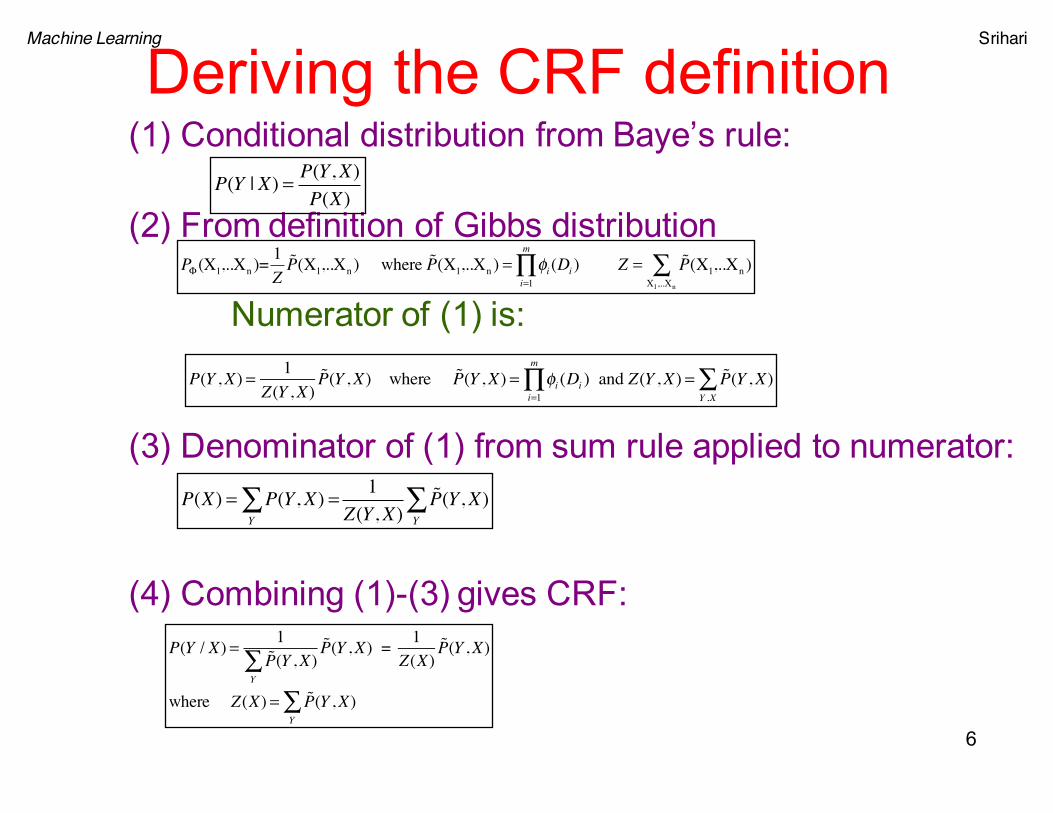
Deriving the CRF definition(1) Conditional distribution from Baye’s rule:

(2) From definition of Gibbs distribution

Numerator of (1) is:

(3) Denominator of (1) from sum rule applied to numerator:

(4) Combining (1)-(3) gives CRF:

6

P(Y | X) = P(Y,X)P(X)

P(Y ,X) = 1

Z(Y ,X)!P(Y ,X) where !P(Y ,X) = φi (Di )

i=1

m

∏ and Z(Y ,X) = !P(Y ,X)Y ,X∑

P(X) = P(Y,X) =Y∑ 1

Z(Y,X)P(Y,X)

Y∑

P(Y / X) = 1!P(Y ,X)

Y∑

!P(Y ,X) = 1Z(X)

!P(Y ,X)

where Z(X) = !P(Y ,X)Y∑

PΦ (X1,..Xn )= 1ZP(X1,..Xn ) where P(X1,..Xn ) = φi

i=1

m

∏ (Di ) Z = P(X1,..Xn )X1,..Xn

∑


Difference between CRF & Gibbs• Different normalization in partition function Z(X)

– A Gibbs distribution

• factorizes into a set of factors and partition function Z– CRF

• Induces a different value of Z for every assignment x to X• Summation only over Y

– Difference denoted by feature variables greyed-out• Known X (shown dark grey)• Y has a distribution dependent on X

7

P(Y | X) = 1Z(X)

P(Y,X) where P(Y,X) = φi (Di )i=1

m

∏ Z(X) = P(Y,X)Y∑

PΦ (X1,..Xn )= 1ZP(X1,..Xn ) where P(X1,..Xn ) = φi

i=1

m

∏ (Di ) Z = P(X1,..Xn )X1,..Xn

∑

(a) (b) (c)

X1

Y1

X2

Y2

X3

Y3

X4

Y4

X5

Y5

X1

Y1

X2

Y2

X3

Y3

X4

Y4

X5

Y5

X1

Y1

X2

Y2

X3

Y3

X4

Y4

X5

Y5


Example of CRF

• CRF over Y={Y1,..Yk} and X={X1,..Xk}• Edges are Yi—Yi+1 and Yi—Xi

8

(a) (b) (c)

X1

Y1

X2

Y2

X3

Y3

X4

Y4

X5

Y5

X1

Y1

X2

Y2

X3

Y3

X4

Y4

X5

Y5

X1

Y1

X2

Y2

X3

Y3

X4

Y4

X5

Y5

P(Y | X) = 1Z(X)

P(Y ,X)

P(Y ,X) = φi (Yi ,Yi+1)i=1

k−1

∏ φi (Yi ,Xi )i=1

k

∏Z(X) = P(Y ,X)

Y∑

Observed Feature Variables:Assumed known when modelis used (hence greyed-out)

Linear chain-structured CRF

For sequence labeling


Main Strength of CRF• Avoid encoding over the variables in X• Allows incorporating into model

– A rich set of observed variables• Whose dependencies are complex or poorly understood

• Allows including continuous variables– Distributions may not have simple parametric forms

• Can incorporate domain knowledge– Rich features without modeling joint distribution

9


CRF Image segmentation

10

car

road

building

cow

grass

(a) (b) (c) (d)Original image Each superpixel isa random variable

Classification using node potentials alone

Segmentation usingpairwise Markov Network encoding

• Each image defines a probability distribution over the variables representing super-pixel labels

• Rather than define joint distribution over pixel values we define a conditional distribution over segment labels given the pixel values

– Avoids making a parametric assumption over (continuous) pixel values– Can define image processing routines to define rich features, e.g.,

presence or direction of an image gradient at pixel» such features usually rely on multiple pixels» So defining correct joint distribution or independence properties over the

features is non-trivial


Directed and Undirected Dependencies

• A CRF defines a conditional distribution of Y on X

• Thus it can be viewed as a partially directed graph

• Where we have an undirected component over Y

• Which has variables in X as parents

11


CRFs for Text Analysis

• Important use for CRF framework• Part-of-speech labeling• Named Entity Tagging

– People, places, organizations, etc• Extracting structured information from text

– From a reference list • Publications, titles, authors, journals, tyear

• Models share a similar structure12


Named Entity (NE) Tagging• Entities often span multiple words• Type of entity may not be apparent from

individual words• New York is location, New York Times is organization

• For each word Xi introduce target variable Yiwhich is its entity type– Outcomes for Yi are (in BIO notation)

• B-PERSON, I-PERSON, B-LOCATION, I-LOCATION, B-ORGANIZATION, I-ORGANIZATION, OTHER

• B: beginning, I: inside entity• B allows segmenting adjacent entities of same type

13


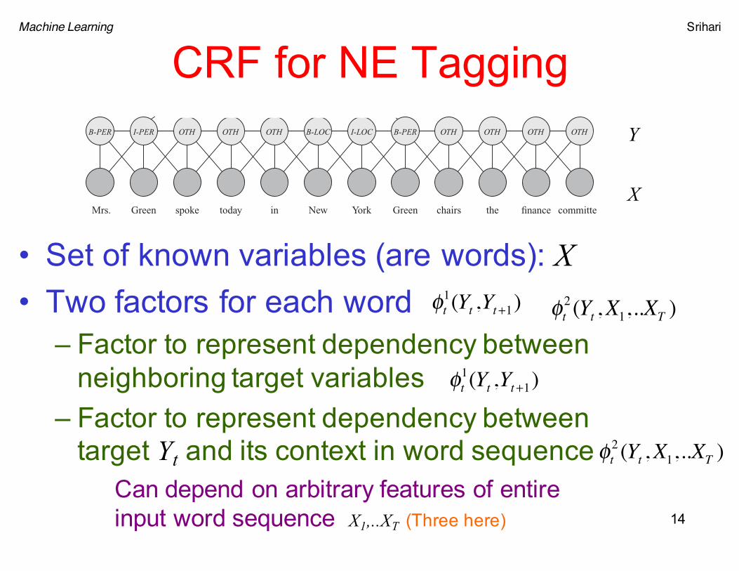
CRF for NE Tagging

• Set of known variables (are words): X• Two factors for each word

– Factor to represent dependency between neighboring target variables

– Factor to represent dependency between target Yt and its context in word sequence

14

Mrs. Green spoke today in New York

(a)

(b)

Green chairs the finance committee

B-PER I-PER OTH OTH OTH B-LOC I-LOC B-PER OTHOTHOTHOTH

its withdrawal from the UALAirways rose after announcing

KEY

Begin person nameWithin person nameBegin location name

B-PERI-PERB-LOC

Within location nameNot an entitiy

I-LOCOTH

British deal

ADJ N V IN V PRP N IN NNDT

B I O O O B I O I

POS

NPIB

Begin noun phraseWithin noun phraseNot a noun phraseNounAdjective

BIONADJ

VerbPrepositionPossesive pronounDeterminer (e.g., a, an, the)

VINPRPDT

KEY

X

Y

φt1(Yt ,Yt+1)

φt2 (Yt ,X1,..XT )

Can depend on arbitrary features of entire input word sequence X1,..XT (Three here)

φt1(Yt ,Yt+1) φt

2 (Yt ,X1,..XT )


Linear Chain CRF for NE• Factor to represent dependency between target

Yt and its context in word sequence– Can depend on arbitrary features of entire input

word sequence X1,..XT

– Not encoded using table factors but use log-linear models• Factors derived from feature functions such as

ft(Yt,Xt)=I{Yt=B-ORGANIZATION,Xt=“Times”}

φt2 (Yt ,X1,..XT )


• For word Xi– Capitalized, In list of common person names,– In atlas of location names, End with “ton”,– Exactly “York”, Following “Times”

• For word sequence – More than two-sports related terms , New York is a sports

organization

• Hundreds or thousands of features• Sparse (zero for most words)

• Same feature variable can be connected to multiple target variables– Yi dependent on identity of several words in window

16

Features for NE Tagging


Performance of CRF

• Linear Chain CRFs provide high per-token accuracies – High 90% range on many natural data sets

• High per field Precision and Recall – Where entire phrase categories and boundaries

must be correct • 80-95% depending on data set

17


Including additional information in NE

• Linear chain graphical model is augmented• When word occurs multiple times in a

document it has the same label• Include factors that connect identical words• Results in skip-chain CRF shown next

18


Skip Chain CRF for NE Recognition

Mrs. Green spoke today in New York

(a)

(b)




KEY


B-PERI-PERB-LOC


I-LOCOTH

British deal


B I O O O B I O I

POS

NPIB


BIONADJ


VINPRPDT

KEY

19

First occurrence of “Green” has neighboring words that provide strong evidence that it is a Person. Second occurrence is more ambiguous.

Augmenting with a long range factorallows to predict correctly.

Graphical structure over Y caneasily depend on the Xs


Joint inference: Part-of-Speech Labeling/Noun-phrase Segmentation Mrs. Green spoke today in New York

(a)

(b)




KEY


B-PERI-PERB-LOC


I-LOCOTH

British deal


B I O O O B I O I

POS

NPIB


BIONADJ


VINPRPDT

KEY

20

Pair of coupled linear chain CRFsNoun phrase is composed of several words that dependson the POS and word


Partially Directed Models• Probabilistic Graphical models are useful for

complex systems:– Directed (Bayesian networks)– Undirected (Markov networks)

• Can unify both representations– Incorporate both directed/undirected dependencies– CRFs can be viewed as partially directed graphs

• CRFs can be generalized to chain graphs– Which have subgraphs with chains

– Network in which undirected components depend upon each other in a directed fashion

21


Directed and Undirected Dependencies

• A CRF defines a conditional distribution of Y on X

• Thus can be viewed as a partially directed graph

22


CRF as Partially Directed Graph• CRF defines a conditional distribution of Y on X

• Can be viewed as one with undirected component over Y which has X as parents

• Factors are defined over Ys only, each of which has an X value

• Equivalent Models 23

(a) (b) (c)

X1

Y1

X2

Y2

X3

Y3

X4

Y4

X5

Y5

X1

Y1

X2

Y2

X3

Y3

X4

Y4

X5

Y5

X1

Y1

X2

Y2

X3

Y3

X4

Y4

X5

Y5

(a) (b) (c)

X1

Y1

X2

Y2

X3

Y3

X4

Y4

X5

Y5

X1

Y1

X2

Y2

X3

Y3

X4

Y4

X5

Y5

X1

Y1

X2

Y2

X3

Y3

X4

Y4

X5

Y5

Linear chain CRF

Equivalent Partially directed variant (CRF)


CRF vs HMM

• Logistic CPDs (logistic regression) is conditional analog of Naïve Bayes

• CRF is conditional analog of HMM

24


Models for Sequence Labeling

Y5

X5

Y5

X5

Y4

X4

Y3

X3

Y2

X2

Y1

X1

Y4

X4

Y3

X3

Y2

X2

Y1

X1

Y5

X5

Y4

X4

Y3

X3

Y2

X2

Y1

X1

(a) HMM (b) MEMM (c) CRF

25

(a) (b) (c)

X1

Y1

X2

Y2

X3

Y3

X4

Y4

X5

Y5

X1

Y1

X2

Y2

X3

Y3

X4

Y4

X5

Y5

X1

Y1

X2

Y2

X3

Y3

X4

Y4

X5

Y5

(a) (b) (c)

X1

Y1

X2

Y2

X3

Y3

X4

Y4

X5

Y5

X1

Y1

X2

Y2

X3

Y3

X4

Y4

X5

Y5

X1

Y1

X2

Y2

X3

Y3

X4

Y4

X5

Y5

MEMM

CRF

HMM

Conditioning on Unknown

Conditioning on Known

P(Y | X) = 1Z(X)

P(Y ,X)

P(Y ,X) = φi (Yi ,Yi+1)i=1

k−1


k

∏Z(X) = P(Y ,X)

Y∑

Generative

Discriminative

P(X,Y ) = P(Xi |Yi )P(Yi+1 |Yi )i=1

k

∏

P(X,Y ) = P(Yi | Xi )P(Yi+1 |Yi )i=1

k

∏

Since Yi s are unknown joint distribution has to be estimated from dataDetermining P(Y|X) depends on first determining P(X,Y)

P(Y|X) is obtained directly


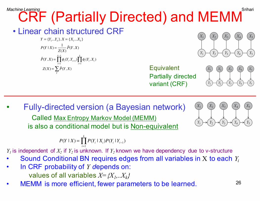
CRF (Partially Directed) and MEMM

26

• Linear chain structured CRF

Partially directed variant (CRF)

• Fully-directed version (a Bayesian network)Called Max Entropy Markov Model (MEMM)

is also a conditional model but is Non-equivalent

Y1 is independent of X2 if Y2 is unknown. If Y2 known we have dependency due to v-structure• Sound Conditional BN requires edges from all variables in X to each Yi• In CRF probability of Y depends on:

values of all variables X={X1,..Xk}• MEMM is more efficient, fewer parameters to be learned.

(a) (b) (c)

X1

Y1

X2

Y2

X3

Y3

X4

Y4

X5

Y5

X1

Y1

X2

Y2

X3

Y3

X4

Y4

X5

Y5

X1

Y1

X2

Y2

X3

Y3

X4

Y4

X5

Y5

(a) (b) (c)

X1

Y1

X2

Y2

X3

Y3

X4

Y4

X5

Y5

X1

Y1

X2

Y2

X3

Y3

X4

Y4

X5

Y5

X1

Y1

X2

Y2

X3

Y3

X4

Y4

X5

Y5

Y = {Y1,..Yk},X = {X1,..Xk}

P(Y | X) = 1Z(X)

P(Y ,X)

P(Y ,X) = φi (Yi ,Yi+1)i=1

k−1


k

∏

Z(X) = P(Y ,X)Y∑ Equivalent

P(Y | X) = P(Yi | Xi )P(Yi |Yi−1)i=1

k

∏

(a) (b) (c)

X1

Y1

X2

Y2

X3

Y3

X4

Y4

X5

Y5

X1

Y1

X2

Y2

X3

Y3

X4

Y4

X5

Y5

X1

Y1

X2

Y2

X3

Y3

X4

Y4

X5

Y5


Models have Trade-offs in expressive power and learnabilityMEMM and HMM are more easily learned

As purely directed models their parameters can becomputed in closed-form using maximum likelihood

CRF requires iterative gradient-basedapproach which is more expensive

Models for Sequence Labeling

Y5

X5

Y5

X5

Y4

X4

Y3

X3

Y2

X2

Y1

X1

Y4

X4

Y3

X3

Y2

X2

Y1

X1

Y5

X5

Y4

X4

Y3

X3

Y2

X2

Y1

X1

(a) HMM (b) MEMM (c) CRF

(a) (b) (c)

X1

Y1

X2

Y2

X3

Y3

X4

Y4

X5

Y5

X1

Y1

X2

Y2

X3

Y3

X4

Y4

X5

Y5

X1

Y1

X2

Y2

X3

Y3

X4

Y4

X5

Y5

CRF

(a) (b) (c)

X1

Y1

X2

Y2

X3

Y3

X4

Y4

X5

Y5

X1

Y1

X2

Y2

X3

Y3

X4

Y4

X5

Y5

X1

Y1

X2

Y2

X3

Y3

X4

Y4

X5

Y5

MEMM

HMM

Later observation has no effect on posterior probability of current state.In activity recognition in video sequence, frames are labelled as running/walking.Earlier frames may be blurry but later ones clearer.

Y1 is independent of X2 if we are not given Y2 More generally, Yi⊥Xj|-X-j

Both CRF and MEMM are Discriminative ModelsThat directly obtain conditional probability P(Y|X)

HMM is a generative model That needs joint probability P(X,Y)

P(X,Y ) = P(Xi /Yi )P(Yi |Yi−1)i=1

k

∏

P(Y / X) = P(X,Y )P(X)

Sequence of observations X={X1,..Xk}. Need a joint label Y={Y1,..Yk}.

P(Y | X) = P(Yi | Xi )P(Yi |Yi−1)i=1

k

∏

Needsjoint

distribution

P(Y | X) = 1Z(X)

P(Y ,X)

P(Y ,X) = φi (Yi ,Yi+1)i=1

k−1


k

∏

Z(X) = P(Y ,X)Y∑


• Binary-valued variables X={X1,..Xk} and Y={Y}– Variables independent of each other and only

dependent on class Y• Pairwise potential between Y and each Xi

• Φi(Xi ,Y)=exp{wi I{Xi=1,Y=1}}• Single node potential• Φ0(Y)=exp{w0 I{Y=1}}

– From CRF definition

CRF Example: Naïve Markov model

I is indicator function which takes value 1 when its argument is true and else 0

P(Y = 1 | x1,..xk ) = exp w0 + wixii=1

k

∑⎧⎨⎩

⎫⎬⎭

P(Y = 0 | x1,..xk ) = exp 0{ } = 1which is equivalent to

P(Y = 1 | x1,..xk ) = sigmoid w0 + wixii=1

k

∑⎧⎨⎩

⎫⎬⎭

where sigmoid(z) = ez

1+ ez

Logistic CPD (regression): not defined by a tablebut induced by parameters. Efficient: Linear (not exponential as in full BN) in the no of parents

X1 X2 Xk

Y


Naïve Markov and Naïve Bayes• Binary variables X={X1,..Xk} and Y={Y}

1. Logistic regression is conditional analog of Naïve Bayes Classifier

1. Naïve Bayes

29

X1 X2 Xk

Y

P(Y = 1 | x1,..xk ) = sigmoid w0 + wixii=1

k

∑⎧⎨⎩

⎫⎬⎭

X1 X2 Xk

Y

P(Y =1| X1,..Xk ) =P(Y =1)

P(Y,X1,..Xk )

P(Y,X1,..Xk ) = P(Y ) P(Xi |Y )i=1

k

∏Generative Model (k parameters): We have to first obtain k CPDs conditioned on unknownfrom which we can get the distribution conditioned on known

Discriminative Model (k parameters)


Properties:A. Symmetryσ(-a)=1-σ(a)

B. Inversea=ln(σ /1-σ)known as logit.Also known as log odds since it is the ratioln[p(Y=1|x)/p(Y=0|x)]

C. Derivativedσ/da=σ(1-σ)

Logistic Regression Revisited• Input X , target classes Y=0 and Y=1• A posteriori probability of Y=1 is

P(Y=1|X) =y(X) = σ (wTX) where

X is a M-dimensional feature vectorσ (.) is the logistic sigmoid function

• Goal: determine the M parameters• Known as logistic regression in

statistics– Although a model for classification

rather than for regression

a

σ(a)

Logistic Sigmoid

Machine Learning


Determining Logistic Regression parameters

• Maximum Likelihood Approach for Two classes

Data set consists of (input,target) pairs: (Xn , tn) where tn ∈ {0,1}, n =1,..,N

Since t is binary we can use the Bernoulli distribution for it

• Likelihood function associated with N observations

where t =(t1,..,tN)T and yn= p(y=1|Xn)

�

p(t |w) = yntn

n=1

N

∏ 1− yn{ }1− tn

31Machine Learning

p(t | w) = yt (1− y)1−t, where y =σ (wtX)


Error Fn for Logistic Regression

Likelihood function

Error function is the negative of the log-likelihood

�

p(t |w) = yntn

n=1

N

∏ 1− yn{ }1− tn

�

E(w) = −ln p(t |w) = − tn ln yn + (1− tn )ln(1− yn ){ }n=1

N

∑

Known as Cross-entropy error function

32Machine Learning


Gradient of Error FunctionError function

where yn= σ(wTXn)

Using Derivative of logistic sigmoidGradient of the error function

�

dσda

= σ(1−σ)

�

E(w) = −ln p(t |w) = − tn ln yn + (1− tn )ln(1− yn ){ }n=1

N

∑

∇E(w) = yn − tn( )n=1

N

∑ Xn

Analytical Derivative:Let z = z1 + z2

where z1 = t lnσ (wtX) and z2 = (1− t)ln[1−σ (t X)]dz1

dw= tσ (wtX)[1−σ (wtX)]X

σ (wtX)anddz2dw

= (1− t)σ (wtX)[1−σ (wtX)](−X)[1−σ (wtX)]

Therefore dzdw

= (σ (wtX)− t)X = (y − t)X

Error x Feature Vector

33

Machine Learning

Contribution to gradient by datapoint n is error between target tnand prediction yn= σ (wTφn) times input Xn

�

ddx(lnax) = a

x


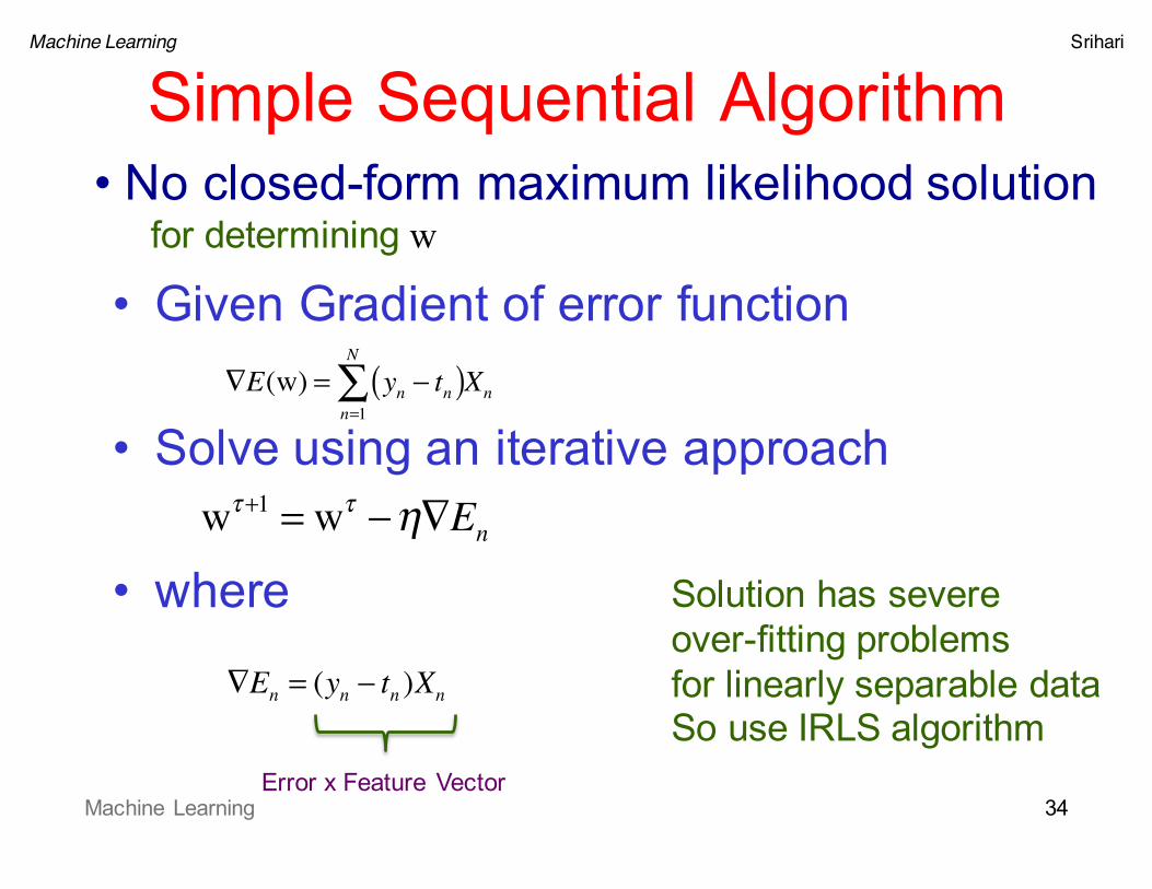
Simple Sequential Algorithm

• Given Gradient of error function

• Solve using an iterative approach

• where

34

wτ+1 = wτ −η∇En

∇En = (yn − tn )Xn

∇E(w) = yn − tn( )n=1

N

∑ Xn

Solution has severeover-fitting problemsfor linearly separable dataSo use IRLS algorithm

• No closed-form maximum likelihood solutionfor determining w

Error x Feature VectorMachine Learning


Multi-class Logistic Regression• Work with soft-max function instead of

logistic sigmoid

where ak=wkTX

35

p(Y = k | X) = yk (X) =exp(ak )exp(aj )j∑

Machine Learning


Muti-class Likelihood Function

• 1-of –K Coding scheme– For feature vector Xn, target vector tn belonging

to class Y=k is a binary vector with all elements zero except for element k

– where ynk=yk(Xn)– T is a N x K matrix of elements with elements tnk

36

p(T | w1,..,wK ) = p(Ck | Xn )tn,k

k=1

K

∏n=1

N

∏ = ynktnk

k=1

K

∏n=1

N

∏

Machine Learning


Multi-class Error Function1. Error Function: negative log-

likelihood

– Known as cross-entropy error function for multi-class

1. Gradient of error function wrt one parameter vector wj

�

E(w1,...,wK ) = −ln p(T |w1,..,wK ) = − tnk ln ynkk=1

K

∑n=1

N

∑

∇w jE(w1,...,wK ) = − (ynj − tnj )Xn

n=1

N

∑

�

∂yk∂a j

= yk (Ikj − y j )

where Ikj are elements of the identity matrix

Derivatives ofSoft-max

yk (X) =exp(ak )exp(aj )j∑

ak=wkTX

Error x Feature VectorMachine Learning


IRLS Algorithm for Multi-class

3. Hessian matrix comprises blocks of size M x M– Block j,k is given by

– Hessian matrix is positive-definite, therefore error function has a unique minimum

4. Batch Algorithm based on Newton-Raphson

Srihari 38

∇wk∇w j

E(w1,...,wK ) = − ynk (Ikj − ynj )Xnn=1

N

∑ XnT

Machine Learning


Iterative Reweighted Least Squares(IRLS)

39

• Efficient approximation using Newton-Raphson iterative optimization

• where H is the Hessian matrix whose elements are the second

derivatives of E(w) with respect to the components of w

�

w(new ) = w(old ) −H−1∇E(w)

Since we are solving forderivative of E(w)Need second derivative

Newton’s Method

SrihariMachine Learning


IRLS Steps• IRLS is applicable to both Linear Regression

and Logistic Regression• We discuss Logistic Regression, for which we

need1. Error function E(w)

• Logistic Regression: Bernoulli Likelihood Function

2. Gradient3. Hessian4. Newton-Raphson update

Srihari 40

�

w(new ) = w(old ) −H−1∇E(w)Machine Learning

�

∇E(w)

�

H = ∇∇E(w)


• Posterior probability of class Y=1 isp(Y=1|X) =y(X) = σ (wTX)

• Likelihood Function for data set {Xn,tn}, tn ∈{0,1}

1. Error Function Log-likelihood yields Cross-entropy

IRLS for Logistic Regression

�

E(w) = − tn ln yn + (1− tn )ln(1− yn ){ }n=1

N

∑

41SrihariMachine Learning

�

p(t |w) = yntn

n=1

N

∏ 1− yn{ }1− tn


2. Gradient of Error Function:

3. Hessian:

Hessian is not constant and depends on w through RSince H is positive-definite (i.e., for arbitrary u, uTHu>0) error function is a concave function of w and so has a unique minimum


∇E(w) = (yn − tn )Xn = XT (y − t)

n=1

N

∑

H = ∇∇E(w) = yn (1− yn )XnXnT = XTRX

n=1

N

∑

R is NxN diagonal matrix with elementsRnn=yn(1-yn)=wTX (1-wTXn)

42Machine Learning


4. Newton-Raphson update:

Substituting and

w(new) = w(old) – (XTRX)-1XT (y-t)= (XTRX)-1{XXw(old)-XT(y-t)} = (XTRX)-1XTRz

where z is a N-dimensional vector with elements z =Xw(old)-R-1(y-t)

Update formula is a set of normal equationsSince Hessian depends on wApply them iteratively each time using the new weight vector


43SrihariMachine Learning

�

w(new ) = w(old ) −H−1∇E(w)∇E(w) = XT (y − t)H = XTRX

Partially Directed Graphs and Conditional Random Fields

Documents

Transcript of Partially Directed Graphs and Conditional Random Fields