Biometrika Trust

Partial Non-Gaussian State SpaceAuthor(s): Neil ShephardReviewed work(s):Source: Biometrika, Vol. 81, No. 1 (Mar., 1994), pp. 115-131Published by: Biometrika TrustStable URL: http://www.jstor.org/stable/2337055 .Accessed: 21/04/2012 15:44

Your use of the JSTOR archive indicates your acceptance of the Terms & Conditions of Use, available at .http://www.jstor.org/page/info/about/policies/terms.jsp

JSTOR is a not-for-profit service that helps scholars, researchers, and students discover, use, and build upon a wide range ofcontent in a trusted digital archive. We use information technology and tools to increase productivity and facilitate new formsof scholarship. For more information about JSTOR, please contact support@jstor.org.

Biometrika Trust is collaborating with JSTOR to digitize, preserve and extend access to Biometrika.

http://www.jstor.org

Biometrika (1994), 81, 1, pp. 115-31 Printed in Great Britain

Partial non-Gaussian state space

BY NEIL SHEPHARD

Nuffield College, Oxford OX1 1NF, U.K.

SUMMARY

In this paper we suggest the use of simulation techniques to extend the applicability of the usual Gaussian state space filtering and smoothing techniques to a class of non- Gaussian time series models. This allows a fully Bayesian or maximum likelihood analysis of some interesting models, including outlier models, discrete Markov chain components, multiplicative models and stochastic variance models. Finally we discuss at some length the use of a non-Gaussian model to seasonally adjust the published money supply figures.

Some key words: EM algorithm; Filtering; Metropolis algorithm; Seasonal adjustment; Smoothing; Unobserved components.

1. MOTIVATION

The Gaussian state space form

Yt = Zt at + st, ?t - N(O, Ht),

a't = Ttat - + Gt it, ilt - N(O, Qt)g (l)

xolYo'-Y..N(a010,Polo) (t=1,. ..,n), where oco I Yo, ?t and il are independent for all t and s and Yt denotes the information available at time t, has had an important role in time series in recent years (West & Harrison, 1989). The columns of Gt will be subsets of the columns of I and are present to ensure that Qt can be assumed to be positive definite even in cases where there are identities in the transition equation. We will also always assume that Ht is positive definite.

Any small modification to the above form, such as removing Gaussianity from one element of Ut, means the Kalman filter and the corresponding smoothing algorithms lose their optimality properties, although occasionally some of the best linear qualities still hold. This leaves the modeller with the difficulty of working with approximate filters, which in turn tend to yield inconsistent parameter estimators.

In this paper we suggest ways of modifying the usual Gaussian filtering and smoothing algorithms to produce exact results. We progress by example, only suggesting a new framework, called a partial non-Gaussian state space, towards the end of the paper. The examples we discuss include outlier models, multiplicative models, discrete Markov chain components, and stochastic variance models. Finally we explore at some length the use of a non-Gaussian model to seasonally adjust the published money supply figures.

2. OUTLIER MODELS

2 1. Student's t distribution We focus on the local level model discussed by Harvey (1989, Ch. 2) and West &

Harrison (1989, Ch. 2), although similar types of results hold for more general unobserved

116 NEIL SHEPHARD

component models. It takes on the form

Yt-= t + t, t at-at_ +ijt9 Ht = 789 Qt = * 2

Suppose we wished to modify this model to allow for outliers. There are two main ways in which this could be achieved: by using a Student's t distribution or a mixture distri- bution. The techniques we use to tackle these two models will be similar. In this section we deal with the former, in the next the latter.

In the Student's ti case, we take (t = e4tl and Ot = r/tl '

instead of et and it/ respectively. Here plW)lt and P2W)2t are independent xP. and xP2 random variables respectively. As Ct and Os are uncorrelated for all t and s, the Kalman filter and smoother will still be best linear estimators; however, they will be poor if Pi or P2 are small.

Initially we assume all the parameters in our models are known. We focus on estimating = (a1 ... , ,j)' and O = (W011, (021'... , in W2n) by reporting the location and scale of

f {(x', W ')'I )Y} = f (b I Yn) say. General solutions to the problem of non-Gaussian state space filtering and smoothing

have been put forward by a number of authors. Kitagawa (1987) suggests sequential approximation using numerical integration rules. This is only feasible if the dimension of the state is very small, 1, 2 or perhaps 3. To cover more complicated situations Kitagawa (1989) has suggested using an approximate Gaussian sum filter (Alspach & Sorenson, 1972; Anderson & Moore, 1979).

More recently there has been a very active interest in methods which allow the pro- duction of simulations from densities like 6 I Yn: see Carlin, Polson & Stoffer (1992), Fruhwirth-Schnatter (1994), Shephard (1993) and unpublished papers by M. West and P. Muiller. Most work is within the Metropolis-Hastings framework, more particularly the single move Gibbs sampler. Ripley (1987, p. 113) and Smith & Roberts (1993) elucidate the ideas behind these techniques.

Unfortunately if 6 I Yn has elements which are highly correlated then the desired asymp- totic distribution of the sampler will only be approached very slowly. To illustrate this point it is useful to work with the Gaussian version of (2). Figure 1 displays the results of a Gibbs sampler for some simulated data with n = 23, a 2 = 1 and a = 5 x 10-5, using 1000 parallel samplers all initialised with OLt = yt/2, recording values after 5, 10, 50, 250, 500 and 1000 iterations. The results show how slowly the Gibbs sampler converges; indeed it is possible to show that the sampler slows as 072 falls, eventually ceasing to converge when 721 = 0. This should not be surprising for the nature of time series modelling is that some of the smoothed estimates of the components, especially estimates of the trend, will be highly correlated through time.

In this paper we suggest that in partial non-Gaussian models it is more useful, as well as simpler, to make many moves simultaneously. The model's block structure, of high correlation within the elements of l I Yn and WoI Yn but low correlation between these two vectors, suggests the following multimove Gibbs sampler, which should be iterated until convergence.

Multimove sampler 1. Generate a candidate point 6 = (', Wo')'. 2. Draw L* from the density f( IW, Yn). 3. Draw W* from the density f(W I o*9 Yn). 4. Write 5 = (oc*', Wo*')' and go to 2.

Convergence will be guaranteed if the joint density of the W1, ... ., W0 is everywhere

Partial non-Gaussian state space 117

0.4 - Truth

-5 --- -10

03~~~~~~5 500 /

ctxl021~~~~ ~ ~ X .0 0-2

0.1

?'?LI-- v , I 5 10 15 20

Time

Fig. 1. Gibbs estimate, after displayed iterations; 'truth' line almost coincides with line for 1000 iterations.

positive (Tierney, 1994). To initialise this sampler, it is only necessary to deal with w, which can often be selected from its unconditional joint distribution, f(c)).

For the outlier model, f(O I co, Yn) and f(ow I x*, Yn) take on particularly attractive forms. We exploit a result which will recur throughout the paper:

n-i

f(cxlw, I~~~)=f(cx.XIw, '1,) HXI 2. .

' f (?' I OJ, Yn) f (L?n I OJ Yn) fl f (Lt ng ?t+ t+2S***Sgn Yn)

t=1

n-i

= f(cxnIw, '( ) H t f 1t ?t?,w Yt). (3) t=1

This is a slight modification of results given recently by Fruhwirth-Schnatter (1994) and Carter & Kohn (1994). In our context this decomposition of the joint density is useful because each expression on the right-hand side involves a Gaussian density, as we have conditioned out all the nonnormality, or in a different context, the nonlinearity, in the system. It turns out that we can solve out each Gaussian density and so, by simulating from each conditional density, we can simulate efficiently from f(L I W, Yn).

We initially focus on implementing this procedure for the simple outlier model. First, given a), the model becomes

Yt = at + Ct 9, t I Ilt - N(O, 0 /w1t)4

Xt = at- 1 + Ot, Ot I 02t N(O, 2 (4)

The last state OL* can be simulated from the density of the conventional Kalman filter xn I O)w Yn N(anIng PnIn) while

r J Pt,t+llt(??x - at+11t) 2_______

at ILx* a,), Yt-N at It + ,P+pt- t +

,I (5) t + pt+11t

9 Ptit Pt+?it J

suggesting that the rest of the <sts can be simulated by progressing backwards, simulating

118 NEIL SHEPHARD

in turn n*- 1 n 2O.C This is easy to program, involving a run of the Kalman filter, which in general takes on the form

at+llt = Tt+latlt-l + Ktvt, Pt+llt = Tt+ Ptlt-lLt + GtQt+1Gl,

vt = Yt - Ztatlti, Ft = ZtPtlt1Z' + Ht, Kt = Tt+1Ptlt-1Z'F-1, Lt = Tt+-

Pt,t+llt = PttT, atlt = atlt + PtltZtF-lvt,

Ptt= Ptt_-Ptt_ ZF1ZtPtl (t = 1, . . ., n), (6)

where

atls = E(octj o_ Ys)q Ptls = Ef(at -at Is)(oct -at Is)' I o, Ys }

Pt,t+llt = Ef(at -at It)(oct + 1-at + 1 t)I a), Yt

The remaining problem is to simulate from n

f(OWLIC*, Yn) H f((ltIYt, at*)f (2t I, Ct-* ) (7) t=l

Since Pi(O1t - ZP1'

{(Yt ~)2 + Pi}WitIYt Oct* Xpl+ (8)

{(4 I)2 + P2} O)2t Ct*- 1 - ZP2 + 12

Hence the simulations from f(w I x'*, Yn) simply involves the drawing of 2n independent x2

variables, while the independence of colt I Yt, oc* and w-)2t I a*q, <t*- 1 suggests that this set-up will yield a rapidly converging sampler.

To illustrate the multimove sampler, a series of length 200 was simulated using Cauchy measurement errors and Gaussian transition errors, with a 2= 1 and aq2 = 0-01. This is displayed in Fig. 2(a). Both Gibbs and multimove samplers were used on these data, running 250 parallel samplers and recording their state estimates after 5, 10, 50, 250, 500, 1000 iterations. The samplers were initialised using the unconditional distribution of the co and ot = yt/2. The results are given in Figs 2(b) and (c). After 5 iterations the multimove sampler is almost exact. This rapid convergence compares favourably with the Gibbs sampler, which is slowed by the high correlation amongst the oc I Yn.

2 2. Gaussian mixture distributions The same type of argument can be used to deal with a time series model whose noise

is drawn from a Gaussian mixture; Harrison & Stevens (1976) call such a structure a multiprocess model. There is a huge literature on this model (Pe-na & Guttman, 1988; Kitagawa, 1989). Most existing solutions to this problem are inexact or involve great computational expense.

Consider the local level model, which will be set up in the following way:

Yt = It + et(olt), et(olt) I olt - N(0, N O2 ),

1t = lt- 1 + t(wt),2t qt(w2t)I2t N(0, I-), (9)

where w1)l and wt2t are independent Bernoulli trials, for all values of t, indexed by probability

Partial non-Gaussian state space 119

(a) Observations

150-

0 50 too 150 200 Time

(b) Gibbs sampler (c) Multimove sampler

o100-

0~~~~~~~~~~~~

0 50 100 1----50 200 0- 0 10 5 0

150

0~~~~~~0

7 0 5015

(bdibsspampl ieratos (c) Multimove ssiae fe ipamp ieratos

12 ~ 2 l62 f l 20_141if0t=

10 -5~~~~~~~~~~~~~~~~~~~

lE22 50 Ct)lt= 1, - 15422 i0 The 8tatistical 250lyisothismodefollwspecislythsamlineasorthStue

2 - 50--50 --1000

0i 0.0 - 5 -10~~-T

0 50 100 150 200 0 50 100 150 200

Time Time

Fig. 2. (a) Simulated series with Cauchy measurement error. (b) Gibbs estimate, after

displayed iterations. (c) Multimove estimate, after displayed iterations.

of success 01 and 02, respectively. The variances in the conditional distributions are given by

2o if w1=, 2 2 fw~O 2~ =

12 ili ()1=0 Et 2 if w =1, th1t =Lr2 if W2 = 1.

Thesttiticl naysi o tismodl olowsprciel the saelnsa2o h tdn'

120 NEIL SHEPHARD

t model, for we can use (3) to simulate from ocx w, Yn, while n

f(Ok x 0*, Yn) = H f (wlt I ?t*, Yt)f(wJ2tI ? -i ). (10) t=1

As

f (0-)lt Iat*q Yt) cf (Yt IO-ltg Lxt*)f (0-)t)9

and the constant of proportionality can be evaluated as colt has discrete support, we can simulate from (10) by drawing 2n uniform random variables.

3. MULTIPLICATIVE MODELS

Suppose that w,tl t1 is Gaussian and not influenced by ox and that the observations and states are linear in co. A simple case of this is

Yt = t)t t + Et, ?t - NID(0, of),

axt =Lat-1 +ijt, ijt-~NID(O, a2), 9l

t = PW)ti- + St, St - NID(0, of),

which might be called a multiplicative state space model. The partially linear structure to this model means the above argument for the Gaussian states can be used again. First, if we condition on the w then the model is a Gaussian state space and so we can simulate LX*. Then, conditioning on the Lx*, the observations and the transition equation for w make up a Gaussian state space and so we can simulate using

n-1

f(OL I LX * , Yn)=f(nIX* In) H f(wtl t?t+x 1*, Yt). (12) t=1

Going to and from one group of states to the next yields a valid sampler so long as p < 1. If p is positive then ocl Yn and wI Yn will be quite correlated and so this sampler may take some time to converge. However, most of the correlation in 6 I Yn has been conditioned out and so it will be much faster than the equivalent single-step Gibbs sampler.

4. MARKOV SWITCHING MODEL

Switching regime models have generated considerable attention in the statistics and econometrics literature. Recently Hamilton (1989) has written about using auto- regressions and a Markov switching regime to model the US business cycle. The use of autoregression allows the computation of the likelihood in a relatively straightforward manner. When the autoregression is replaced by ARMA or unobserved components, this approach no longer works.

To focus ideas we will again exploit a simple model with

Yt = ct + stSsEt - NID(O, a2), ct= cxt +y +#ot + t, ut - NID(O, U2). (13)

Here et and Us are independent from the w, process for all t, s and u. wt is assumed to be a binary Markov chain, with transition probabilities

O)t = ? 0)t = 1

0)t- 1 = ? i (- 01 1 8 ( 14)

Partial non-Gaussian state space 121

The motivation for this model is that the slope of the trend is either y or y + f,, which in the US GDP case corresponds to a recession or boom. The slope state, (w, shifts with probabilities controlled by 01 and O2

The simulation from cxlw, Yn can be carried out using (3). Using (12), the drawing of random variables from co X c*, Yn is also straightforward for the filtering equations take on the form, if we write at = (gx, * * *, ax)t,

pr (wt I cc' - 1, Yt - ) = pr (wt I' ot) - 1) t- pr (wt I wt_ - pr (wt_ - 1 1 ot- ), (15)

pr (wt Ixt, Yt) = pr (wt I t) oc pr (at, xt- 1 1 Wt) pr (wt Ict - 1).

This is soluble because of the discrete support of wt, which means the summation and the constant of proportionality can be evaluated. These equations allow pr (wnlo *, Yn) to be computed. All that is additionally required is the calculation

pr (wt l wt + 1, *, Yn) oc pr (wt I x*t) pr (wt + 1 i wt).

5. STOCHASTIC VARIANCE MODELS

The stochastic variance model is given by

Yt = Et exp (ct/2), et NID(O, 1), (16)

at= qt_1

+ t, t tNID(O, u2).

This model is a discrete time approximation to a model which is highly motivated in the finance literature. It is used to generalise the Black-Scholes option pricing equation to allow the variance to change over time (Hull & White, 1987; Chesney & Scott, 1989; Melino & Turnbull, 1990).

The transformation

log y2 = at + log e6,

gives a linear but non-Gaussian state space. Harvey, Ruiz & Shephard (1994) employed a Kalman filter to estimate the unobservable states and a quasi-likelihood to perform parameter estimation. This is suboptimal as log e' is far away from its normal approxi- mation N(- 1 2704, 4 9348), which in turn means the implied quasi-likelihood estimator has poor small sample properties.

Here we approximate the density of zt = log e', the log X' distribution, by a mixture density

K

fz( ( Z) E )Z ci (Z | c ) (17) i=1

where zI o N (d - 1 2704, a2). We select )',. ..., w, Kt1,,1K... ltK and U2 to make the approximation 'sufficiently good'. In practice, we might make the first 4 or 6 moments agree exactly and require that the approximating density lie within a certain distance of the true density. See Titterington, Smith & Makov (1985, p. 133) for the appropriate techniques.

Clearly,

log yt2 O)t, axt - N(at - 1 2704 + wt, a.2) (18)

where w denotes the single element of c, ... ., CK corresponding to time t. We can sample

122 NEIL SHEPHARD

from oc I , Y1', which has the same distribution as oc I, X,,, where X,, = (log y',... , log y2)'. The second part of the multimove sampler requires us to simulate from

n n

f( X*, Xn) =Hf (tI I oC, log y2) H f(log yt2|, cX*)ft(t). (19) t=1 t=1

We can simulate from w log y2, * using a rejection algorithm, drawing with replacement w) from wl, ... ., OK with probability 7E1,... CK respectively.

6. PARTIAL NON-GAUSSIAN STATE SPACE

All the models discussed above, and many more, fit within the following framework which we call the partial non-Gaussian state space:

Yt = Zt(o)t)oxt + dt(o)t) + et(ot), et(o)t)l ot - N{0, Ht(jw)}, (20)

at = Tt(ot)ct- 1 + ct(ot) + uit(o), ,t(ot) I ot - N{0, QtJ(o)}, (20

where w = (w', ... , wO)' is a Markov process, that is

n

f (0) I )0) = fl f (O)t I )t -1). (21) t=1

Throughout, et(t) I ot and U,(w) I o) are assumed independent of one another for all values of t and s.

This framework allows the introduction of non-Gaussianity and nonlinearities into the model while still allowing a certain ease of analysis. It is a special case of the set-up suggested by Kitagawa (1987). However, unlike Kitagawa's model, this approach does not exhibit a prohibitive computational explosion as the size of the state, oct, expands.

The smoothing density 6 I Yn 5 where 6 = (oc', a')', can be simulated using a multimove sampler. The first step is to draw from c I w, Yn. As before

n-1

f(CXlw Yn) =f(oXnIw Yn) H X f IcXt?+ 1 (, Yt), (22) t=1

which are all Gaussian densities. The first of them, f(oCXn , Yn), is given by the Kalman filter, (6), while

atIat* 1, w, Yt - N{at +

+1-+ltP t+l lt((x*+l-at+1it), Ptlt -Pt,t+

,tP-1 tPt+,lt

l (23)

can be found from a single run of the Kalman filter. Computationally the only problem is that, at each t = n - 1, n -2 ... . 1, we have to compute the inverse of Pt+ 1t, a matrix the dimension of the state vector.

This result implies that cx I w, Yn can be simulated routinely. The task of simulating from w Io , Yn is not so easy in general, but there are some special cases where a relatively complete solution can be offered.

One case is where wtlwt-, is non-Gaussian but where, given o*, the model has a conjugate filter for w. A class of models which possess this property is based on the gamma-beta transition models suggested by Smith & Miller (1986). An example of this is Shephard's (1994) local scale model. This will be illustrated by

Yt = ct + ej#t), e-It I ot- N(O, o7- 1) ct = at-1 + llo It n NID(0O, (24)5

Partial non-Gaussian state space 123

where at1 is defined in (25). Here the logarithm of the measurement equation precision follows a random walk. Then

OtIo(*, Yt - G(at, bt), at = (Aat t-1il) + 1, bt = (e-rtbt_-lt_-) + 1(yt - c*)2. (25)

We can use a rejection algorithm to simulate from

f (oIt I t*+ 1 o (* Yt) ocf (oit I It* Yt)f(0t*+ 1 I w), (26) which is straightforward using a gamma random number generator.

Thus results on simple conjugate time series models can be exploited inside quite compli- cated models, widening their use.

For more general f(wt I t- 1), the following cases may be useful.

Case 6-1: ot are serially independent. We can simulate from n n

f(Lx ) I X n) = H f (otIx?,t I -x , Yt) Hc 1 f(yt I cx, o)t)f (xI|-1, Ia t)f(o)t) (27) t=l t=l

using a rejection algorithm if we can boundf(yt I ?C*, wt)f(xc* I a* 1, wt). If this is not possible then we can fall back on the use of the Metropolis algorithm.

Case 6 2: Univariate general case. In general for a nonconjugate OtIo -o we can use a single-step Gibbs sampler based on the conditionals

f (O-t IO-t*-1 O-t + 1 ?5 CX* Yn) = f(O-t IO-t*-1 5 O-t + 1 Xt*-1 5 CXt* 5 Yt)

oc f Yt, cxt*- l, a t* I (ot f ((t I (ot*- l,5 ot + 1)

o f ( Yt I c xt* O-)t ) f( c t* c x t*- 1 5 O-)t ) f(O(t + 1 I -) t ) f( O)t I o t*- 1 ) 5 (28 ) working our way forwards through the data, simulating 01, ... ., On in turn. Ways of carrying out rejection sampling from densities such as these are discussed by Carlin et al. (1992). When this is not directly possible then the Metropolis algorithm can be used (Shephard, 1993).

When wt is multidimensional the problems of drawing random variables from the relevant densities becomes much harder and probably should be addressed on a case by case basis.

7. ESTIMATION USING SIMULATION

7 1. The states Having obtained M replications from 6 I Yn 5 perhaps M consecutive realisations from

the multistep sampler which will not be independent, we need to be able to estimate the characteristics of xtI Yn and otI Yn. We write the ith replication of wI Yn as w(). A density estimator of xtI Yn iS

M

M-1 YE f(CXt IOJ(i)5 Yn)5 i=1

while the corresponding mean, E(xt I Yn), can be estimated by M

M -1 E(xt Io-(')5 Yn). i=l

Since oc() Y 1 is Gaussian there exist exact smoothing algorithms for the mean and

124 NEIL SHEPHARD

variance of this distribution. Following a single pass of the Kalman filter, the backwards smoothing recursions take on the form

etln = Yt - Ztatln ntln = atln--Tatj1n atln = atlt-l + Ptlt-lrt-1,

P = P l-Ptjt_jNt_jPtjt_ , rt1 = ZtF71vt + L'rt, Nt-V = ZtF7'Zt + L'NtLt

(29)

(De Jong, 1989). The Kalman filter will already have been run in order to carry out the simulations of cx w, Yn and so this adds no extra burden. The smoothing algorithms here are more computationally involved than the Kalman filter; however the cost of running them is still small compared to the expense of the drawing of the simulations.

In general, analytic smoothing algorithms for wlxo*, Y1' will not exist and so simpler averages of the replications (i) will sometimes have to be used in reporting summaries of 1 Yn.

7-2. One-step ahead prediction densities The likelihood is given by

n f(Y1, * **,Yn1Y0;O)= f[f(Yt1Yt-1; 0)

t=1

Also

f(YtlI Yt- 1; 0) f W(ytI lQt- 1 Yt- 1; O)f (ft- 11 Yt- 1) MQt- 1 (30)

where nt -1 = (o)1, . . . , - i)'. J As we can use multimove sampling to draw from t -'1 Y - 1 we can estimate (30) by

M M- 1 f f(yt I9t(i) 1 , Yt - 1; 0)9

where n(i) 1 are the simulated values. Recall that f(yt I ) 1 Yt 1; 0) has a simple form for Yt I lt, t-1, is Gaussian and its mean and variance are given by the Kalman filter (6).

As t increases we have to lengthen 0 and each iteration of the Gibbs sampler, in effect, performs a Kalman filter. Thus direct likelihood evaluation may not be the most compu- tationally efficient way of maximising the likelihood. However, it is still useful to compute the likelihood to gauge the fit of the model, as well as to allow simple hypothesis testing. Further, the one-step ahead prediction densities are useful for diagnostic checking. These points will be illustrated in ? 9.

8. PARAMETRIC ESTIMATION

8 1. General It is important to present methods which deal effectively with the unknown parameters

0. We discuss two ways; a Bayesian approach and a simulated EM algorithm. The Bayesian approach has been well documented elsewhere (Smith & Roberts, 1993),

and so we discuss it only briefly here. It requires the specification of a prior over 0, written f0(O). Then the multimove sampler is amended as follows:

Partial non-Gaussian state space 125

Multimove Bayesian sampler 1. Generate a candidate point 3 = (oc', a', 0')'. 2. Draw o* from the density f(c I w, 0, Yn). 2. Draw w* from the density f(w I oc*, 0, Yn). 4. Draw 0* from the density f(0 Io)*, c*, Yn). 5. Write 3 (a*', w*', 0*')' and go to 2.

This sampler will converge to replications from 6 I Yn which will contain drawings from the posterior density 01 Yn. The posterior density can be estimated by

M M-1 YE f(oO IO)i), 2(i), Yn

i=l

If fo(0) is flat, this estimate can be used to find the maximum likelihood estimator.

8 2. EM algorithm An alternative approach to find the maximum likelihood estimator uses an EM algor-

ithm. This follows naturally from using smoothing techniques. Recall

log f (yI YO; 0) = log f (, I YO; 0) -log f (b Yn; 0), (31)

so that integrating both sides with respect to the smoothing density f(b I Yn; O%, where O' is some arbitrary point, gives

109 f(yn I YO; 0) = Q (f0 ffil Yn) -H(05, Oil Yn)5 (32) where

Q(0, Oil Yn) = flogf(65 Yn I YO; O)f(bI Yn; 0') d3, (33)

H(0, 0il Yn) = flogf(b I Yn; 0)f(b I Yn; Qi) db. (34)

The usual EM algorithm argument (Dempster, Laird & Rubin, 1977) implies that, if we select Q0+1 so that Q (0, oil Yn) is maximised with respect to 0, then

109 f ( yn I YO; Oi ) ) log10 f ( yn I YO; Oi)-

Iteration leads to the maximisation of the likelihood. Using the structure of the general partial non-Gaussian state space we can solve some

of these integrals analytically. We write

Q(0, Oil Yn) = JR(05 0'lc, Yn)f(wI Yn; Oi) do + Jlogf(w); 0)f(woI Yn; Oi) do), (35)

where

R(0, Ol, ') Yn= flogf(YnI, I w, YO; 0)f(xcxIo, Yn; Oi) dox (36)

(Harvey, 1989, p. 188). We focus on the special case where all the parameters in the Gaussian measurement and transition equations are in the matrices Ht and Qt. Then,

126 NEIL SHEPHARD

suppressing dependence on w, we can follow Koopman (1993) in writing

1 n 1 n

R(,5O')= - E log 1H(0)1-- E tr [H,()1 fe,lne'ln+cov (E- e,n)1] 2 t12 t= t=1 t=1

1n 1n - E Z log IQt(0)l - - Z tr [Qt(0)-1 {nt1n;n + cov ('t-ntln)}], (37) 2 t=l 2 t=1

where E(et I, 5Yn) =et In and E(tI, Yn) = ntn. These terms, and the others in the above formula, are computed recursively through

etln = Htet, cov (et - etln) =Qtrt- 38

ntln=H -HD H cov (t(-ntln) 3Qt8-QtNt-)Qt

where they are calculated by first running the Kalman filter, (6), and then starting with rn = 0 and Nn = 0 using the backwards recursions

et= F-lvt-Krt, rti = Z'F-1vt + L'rt, D~=F7'+N~K~, N1=ZF7'Z+LNtLt .(39) Dt=F-1 + K'NtKt, Nt-, = Z'Ft-'Zt + LtNtLt.

Throughout the recursions and the associated Kalman filter, 0 is taken to be W'.

8 3. Simulated EM algorithm We can estimate Q(0, Oil Yn) by using simulations from o I Yn; Wi. Simulated EM algorithms

have been used by, amongst others, Bresnahan (1981), Celeux & Diebolt (1985), Wei & Tanner (1990), Tanner (1991), Qian & Titterington (1991) and Shephard (1993). So

Q(0, o'l Yn) = - Z {R(05, Oldii), Yn) + log1f(0O); O)}, (40)

which is usually easy to manipulate. Typically the parameter space splits so that we can work with 0 = (x',, ')' so that

I M

Q(0, O'l Yn)= - Z {R(Z, Oilo(J)5 Yn) + log f(c(j1; u1)}, (41)

in which case the maximisation will be particularly straightforward. In some special cases -u may be a null set: this is true, for instance, in the stochastic variance model discussed in ? 3. A similar type of argument can be used to deliver a direct estimator of the score vector (Koopman & Shephard, 1992).

9. NONLINEAR SEASONAL ADJUSTMENT

We illustrate the techniques suggested above by modelling the quarterly changes of M4 in the UK from 63Q2 to 82Q4 in Fig. 3(a); a series used in the Bank of England's 1992 report on seasonal adjustment procedures. The Bank's report compares three seasonal adjustment procedures: an in house moving average scheme, the US Bureau of the Census' Xll and a model based seasonal adjustment procedure which fits a Gaussian unobserved component model (Harvey, 1989, pp. 300-9). We focus on the last of these, to compare its fit with a new non-Gaussian model we propose.

Partial non-Gaussian state space 127

(a) M4 (b) Log M4

6 0003

5-

0.02-

0~~~~~~~~~~~~00 2) -

0 0.00

0 20 40 60 80 0 20 40 60 80 Time Time

Fig. 3. Quarterly changes (a) in UK first difference M4 (? billions): 63Q2 to 82Q4, and (b) in log of first difference M4.

The Gaussian model fitted to M4 was

Yt = lit + yt + t, -Pt - NID(0, r2),

it= pt_ + /t1 + qt - NID(O, c2), (42)

At= f-1 + 't, St - NID(0, f2),

Tt = -Tt-1 * -t-3 + O)t5 0) - NID(O, 52O

Here et Y, Su and w, are assumed independent for all t, s, u and v. The maximum likelihood estimates of the parameters are

ag = 021, 0i2=O0041, 6 = 0000007, 6O = 0020, log L(O) =-79, (43)

while the standard innovations-based diagnostic statistics (Harvey, 1989, pp. 258-60) take on the values

S = 0 20, K = 4412, N(X2) = 4-39, Qlo (X2) = 9.75, H24(F24,24)

= 17 1. (44)

These statistics refer to skewness, kurtosis, normality, serial correlation measured by the Box-Ljung statistic and heteroscedasticity, respectively. The diagnostics are satisfactory except the model allows too much variability in the initial part of the series while not allowing enough at the end. This is picked up in Fig. 4(a) and by the heteroscedasticity statistic H24.

Figure 3(b) gives differences of the logged series. This is convenient as this transform- ation approximately equals the proportional change, which is probably the statistic of most interest. The innovations from fitting (42) to Fig. 3(b) are given in Fig. 4(b). Although they show some minor improvements over Fig. 4(a), they are still very poor. The diagnostic statistics and estimated components from this model are very similar to those of the linear

128 NEIL SHEPHARD

(a) Innovations, linear (b) Innovations, log

2 -

0,010 0

4-a ~2 40a 60 8020 40 60 8

o o~~~~~~~~~~~~~~~'

0 ~~~~~~~20.005

CeTYim Time

C- 11.11t Hjtj 1ii4 +II C,C IDO r

*t =-.t 1-_ -t-3+O* O*~NDO 2*

-0-005

uni e (42), (45 liiib ad ttoar ytasfrain

-0-010

-2

20 40 60 80 20 40 60 80 Time Time

Fig. 4. Innovations (a) from linear model and corresponding 95% intervals, (b) from log- linear models and 95% intervals.

model. To try to improve the fit of the linear model we exploit a mixed multiplicative- additive unobserved component model. The model we use is

wheres required diandibutare.assumedcindependenttefor allvt,gs,cu,wv,lidand]. Noticelthat

ule2 a (42) (45)e cannotibemade stationarym ba y transforma

The sitemulatipMlicaitive seasoa effect and penfrprmtersh moelstiapootion, movingn

?I ~~~~~(45)

wheest of the irreul ad_arcmoen hass goned indepndet* frc allouts for u the land ge Noincretase

inthe l*iseiodoe h iermdl h aineo the multiplicative seasonal efcanetrshemdlsapootion moving

the trend up and down by scaling. The total seasonal effect is o Likewise the irregular term in this model is I.tes' +,et, making it heteroscedastic.

This is an example of the multiplicative models discussed briefly in ? 3. We can write Ot= (Vt* V Tt- i, V T- 2 9'St*)' to place the model into its partial non-Gaussian state space. So

long as the variances are all strictly positive the multistep Gibbs sampler will converge to its required distribution. In practice the rate of convergence will depend crucially on

a,a low value rendering the algorithm relatively slow. The simulated Em algorithm was used to perform parameter estimation, yielding

0 O004, 0 =O0949 2 0-01,9~ 0.00005, 0-* 003, log L(O)=- 62.

(46)

Most of the irregular component has gone into s* which accounts for the large increase in the likelihood over the linear model. The variance of the multiplicative seasonal is lower

Partial non-Gaussian state space 129

(a) Innovations, nonlinear (b) Uniform innovations

10 _ 3

2 ~~~~~~~0.8 co n

O4a

TiII IT 11 0 ~ ~ ~ ~ ~ ~~~0

4-a I~I 0.2

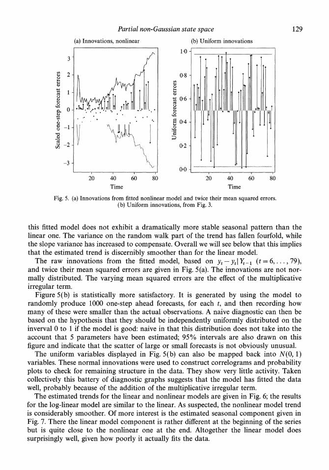
Fig. 5. (a) Innovations from fitted nonlinear model and twice their mean squared errors. (b) Uniform innovations, from Fig. 3.

this fitted model does not exhibit a dramatically more stable seasonal pattern than the linear one. The variance on the random walk part of the trend has fallen fourfold, while the slope variance has increased to compensate. Overall we will see below that this implies that the estimated trend is discernibly smoother than for the linear model.

The raw innovations from the fitted model, based on Yt -Yt It-l (t =6,... ,79), and twice their mean squared errors are given in Fig. 5(a). The innovations are not nor- mally distributed. The varying mean squared errors are the effect of the multiplicative irregular term.

Figure 5(b) is statistically more satisfactory. It is generated by using the model to randomly produce 1000 one-step ahead forecasts, for each t, and then recording how many of these were smaller than the actual observations. A naive diagnostic can then be based on the hypothesis that they should be independently uniformly distributed on the inverval 0 to 1 if the model is good: naive in that this distribution does not take into the account that 5 parameters have been estimated; 95%/ intervals are also drawn on this figure and indicate that the scatter of large or small forecasts is not obviously unusual.

The uniform variables displayed in Fig. 5(b) can also be mapped back into N(0, 1) variables. These normal innovations were used to construct correlograms and probability plots to check for remaining structure in the data. They show very little activity. Taken collectively this battery of diagnostic graphs suggests that the model has fitted the data well, probably because of the addition of the multiplicative irregular term.

The estimated trends for the linear and nonlinear models are given in Fig. 6; the results for the log-linear model are similar to the linear. As suspected, the nonlinear model trend is considerably smoother. Of more interest is the estimated seasonal component given in Fig. 7. There the linear model component is rather different at the beginning of the series but is quite close to the nonlinear one at the end. Altogether the linear model does surprisingly well, given how poorly it actually fits the data.

130 NEIL SHEPHARD

6-

Ce

Ce 2

0- o- I * * * ** *~~~~~~~I

0 20 40 60 80 Time

Fig. 6. Actual and estimated trend, linear (solid line) and nonlinear (dotted line).

0

-1

0 20 40 60 80

Time

Fig. 7. Estimated seasonal pattern, linear (points) and nonlinear (dotted line).

ACKNOWLEDGEMENTS

The author would like to thank the referee and the editor for their detailed and very constructive comments on the previous versions of this paper and Robert Kohn and Brian Ripley for some useful discussions. This research was supported by a grant from the ESRC.

REFERENCES

ALSPACH, D. L. & SORENSON, H. W. (1972). Nonlinear Bayesian estimation using Gaussian sum approxi- mations. IEEE Trans. Auto. Control AC-17, 439-48.

Partial non-Gaussian state space 131

ANDERSON, B. D. 0. & MooRE, J. B. (1979). Optimal Filtering. Englewood Cliffs: Prentice-Hall. BRESNAHAN, T. F. (1981). Departures from marginal-cost pricing in the American automobile industry, esti-

mates from 1977-1978. J. Economet. 17, 201-27. CARLIN, B. P., POLSON, N. G. & STOFFER, D. (1992). A Monte Carlo approach to nonnormal and nonlinear

state-space modelling. J. Am. Statist. Assoc. 87, 493-500. CARTER, C. K. & KoHN, R. (1994). On Gibbs sampling for state space models. Biometrika 81. To appear. CELEUX, G. & DIEBOLT, J. (1985). The SEM algorithm: a probabilistic teacher algorithm derived from the EM

algorithm for the mixture problem. Computat. Statist. Quart. 2, 73-82. CHESNEY, M. & SCOTT, L. 0. (1989). Pricing European options: a comparison of the modified Black-Scholes

model and a random variance model. J. Financ. Qualitat. Anal. 24, 267-84. DE JONG, P. (1989). Smoothing the interpolation with the state space model. J. Am. Statist. Assoc. 84, 1085-8. DEMPSTER, A. P., LAIRD, N. M. & RUBIN, D. B. (1977). Maximum likelihood from incomplete data via the

EM algorithm. J. R. Statist. Soc. B 39, 1-38. FRUHWIRTH-SCHNATTER, S. (1994). Data augmentation and dynamic linear models. J. Time Ser. Anal. 15,

183-202. HAMILTON, J. (1989). A new approach to the economic analysis of nonstationary time series and the business

cycle. Econometrica 57, 357-84. HARRISON, J. & STEVENS, C. F. (1976). Bayesian forecasting (with discussion). J. R. Statist. Soc. B 38, 205-47. HARVEY, A. C. (1989). Forecasting, Structural Time Series Models and the Kalman Filter. Cambridge

University Press. HARVEY, A. C., Ruiz, E. & SHEPHARD, N. (1994). Multivariate stochastic variance models. Rev. Econ. Stud.

61. To appear. HULL, J. & WHITE, A. (1987). Hedging the risks for writing foreign currency options. J. Int. Money Finance

6, 131-52. KITAGAWA, G. (1987). Non-Gaussian state space modelling of non-stationary time series. J. Am. Statist. Assoc.

82, 503-14. KITAGAWA, G. (1989). Non-Gaussian seasonal adjustment. Comp. Math. Applic. 18, 503-14. KOOPMAN, S. J. (1993). Disturbance smoother for state space models. Biometrika 80, 117-26. KOOPMAN, S. J. & SHEPHARD, N. (1992). Exact score for time series models in state space form. Biometrika

79, 823-6. MELINO, A. & TURNBULL, S. M. (1990). Pricing foreign currency options with stochastic volatility. J. Economet.

45, 239-65. PENA, D. & GUTTMAN, L. (1988). Bayesian approach to robustifying the Kalman filter. In Bayesian Analysis

of Time Series and Dynamic Models, Ed. J. C. Spall, pp. 227-54. Cambridge, Mass.: Marcel Dekker. QIAN, W. & TITTERINGTON, D. M. (1991). Estimation of parameters in hidden Markov Chain models. Phil.

Trans. R. Soc. Lond. A 337, 407-28. RIPLEY, B. D. (1987). Stochastic Simulation. New York: Wiley. SHEPHARD, N. (1993). Fitting non-linear time series models, with applications to stochastic variance models.

J. Appl. Economet. 8, 5135-58. SHEPHARD, N. (1994). Local scale model: state space alternative to integrated GARCH processes. J. Economet.

60, 181-202. SMITH, A. F. M. & ROBERTS, G. (1993). Bayesian computations via the Gibbs sampler and related Markov

Chain Monte Carlo methods. J. R. Statist. Soc. B 55, 3-23. SMITH, R. L. & MILLER, J. E. (1986). A non-Gaussian state space model and application to prediction records.

J. R. Statist. Soc. B 48, 79-88. TANNER, M. A. (1981). Tools for Statistical Inference, Observed Data and Data Augmentation Methods, 67.

New York: Springer-Verlag. TIERNEY, L. (1994). Markov Chains for exploring posterior distributions. Ann. Statist. 22. To appear. TITTERINGTON, D. M., SMITH, A. F. M. & MAKOV, U. E. (1985). Statistical Analysis of Finite Markov

Distributions. Chichester: Wiley. WEI, G. C. G. & TANNER, M. A. (1990). A Monte Carlo implementation of the EM algorithm and the poor

man's data augmentation algorithms. J. Am. Statist. Assoc. 85, 699-704. WEST, M. & HARRISON, J. (1989). Bayesian Forecasting and Dynamic Models. New York: Springer-Verlag.

[Received February 1993. Revised August 1993]