Cop

yrig

ht ©

201

4 U

nive

rsity

of C

ambr

idge

. Not

to b

e qu

oted

or

repr

oduc

ed w

ithou

t per

mis

sion

.

Partial Differential Equations Example sheet 4

David Stuartdmas2@cam.ac.uk

4 Parabolic equations

In this section we consider parabolic operators of the form

Lu = ∂tu + Pu

where

Pu = −n∑

j,k=1

ajk∂j∂ku +n∑

j=1

bj∂ju + cu (4.1)

is an elliptic operator. Throughout this sectionajk = akj, bj, c are continuous functions,and

m‖ξ‖2 ≤n∑

j,k=1

ajkξjξk ≤ M‖ξ‖2 (4.2)

for some positive constantsm,M and allx, t andξ. The basic example is the heat, ordiffusion, equationut − ∆u = 0 , which we start by solving, first forx in an intervaland then inR

n. We then show that in both situations the solutions fit into anabstractframework of what is called asemi-group of contraction operators. We then discusssome properties of solutions of general parabolic equations (maximum principles andregularity theory).

4.1 The heat equation on an interval

Consider the one dimensional heat equationut − uxx = 0 for x ∈ [0, 1], with Dirich-let boundary conditionsu(0, t) = 0 = u(1, t). Introduce the Sturm-Liouville operatorPf = −f ′′, with these boundary conditions. Its eigenfunctionsφm =

√2 sin mπx con-

stitute an orthonormal basis forL2([0, 1]) (with inner product(f, g)L2 =∫

f(x)g(x)dx,considering here real valued functions). The eigenvalue equation isPφm = λmφm withλm = (mπ)2. In terms ofP the equation is:

ut + Pu = 0

and the solution with initial data

u(0, x) = u0(x) =∑

(φm, u0)L2φm ,

Cop

yrig

ht ©

201

4 U

nive

rsity

of C

ambr

idge

. Not

to b

e qu

oted

or

repr

oduc

ed w

ithou

t per

mis

sion

.

is given byu(x, t) =

∑e−tλm(φm, u0)L2φm . (4.3)

(In this expression∑

means∑∞

m=1.) An appropriate Hilbert space is to solve foru(·, t) ∈ L2([0, 1]) given u0 ∈ L2, but the presence of the factore−tλm = e−tm2π2

means the solution is far more regular fort > 0 than fort = 0:

Theorem 4.1.1 Let u0 =∑

(φm, u0)L2φm be the Fourier sine expansion of a functionu0 ∈ L2([0, 1]). Then the series(4.3)defines a smooth functionu(x, t) for t > 0, whichsatisfiesut = uxx and limt↓0 ‖u(x, t) − u0(x)‖L2 = 0.

Proof Term by term differentiation of the series with respect tox, t has the effect onlyof multiplying by powers ofm . For t > 0 the exponential factore−tλm = e−tm2π2

thus ensures the convergence of these term by term differentiated series, absolutely anduniformly in regionst ≥ θ > 0 for any positiveθ . It follows that for positivet the seriesdefines a smooth function, which can be differentiated term by term, and which can beseen to solveut = uxx . To prove the final assertion in the theorem, choose for eachpositiveǫ, a natural numberN = N(ǫ) such that

∑∞N+1(φm, u0)

2L2 < ǫ2/42 . Let t0 > 0

be such that for|t| < t0

‖N∑

1

(e−tλm − 1)(φm, u0)L2φm‖L2 ≤ ǫ

2.

(This is possible because it is just a finite sum, each term of which has limit zero). Thenthe triangle inequality gives (for0 < t < t0):

‖u(x, t) − u0(x)‖L2 ≤ ‖∞∑

1

(e−tλm − 1)(φm, u0)L2φm‖L2

≤ ǫ

2+ 2 × ‖

∞∑

N+1

(φm, u0)L2φm‖L2 ≤ ǫ

which implies thatlimt↓0 ‖u(x, t)−u0(x)‖L2 = 0 sinceǫ is arbitrary. (In the last bound,the restriction tot positive is crucial because it ensures thate−tλm ≤ 1.) 2

Theinstantaneous smoothingeffect established in this theorem is an important prop-erty of parabolic pde. In the next section it will be shown to occur for the heat equationon R

n also.The formula (4.3) also holds, suitably modified, whenP is replaced by any other

Sturm-Liouville operator with orthonormal basis of eigenfunctionsφm. For example,for if Pu = −u′′ on [−π, π]) with periodic boundary conditions: in this caseλm = m2

andφm = eimx/√

2π for m ∈ Z .

4.2 The heat kernelThe heat equation isut = ∆u where∆ is the Laplacian on the spatial domain. For thecase of spatial domainRn the distribution defined by the function

K(x, t) =

1√

4πtnexp[−‖x‖2

4t] if t > 0,

0 if t ≤ 0,(4.4)

2

Cop

yrig

ht ©

201

4 U

nive

rsity

of C

ambr

idge

. Not

to b

e qu

oted

or

repr

oduc

ed w

ithou

t per

mis

sion

.

is the fundamental solution for the heat equation (inn space dimensions). This canbe derived slightly indirectly: first using the Fourier transform (in the space variablexonly) the following formula for the solution of the initial value problem

ut = ∆u , u(x, 0) = u0(x) , u0 ∈ S(Rn) . (4.5)

Let Kt(x) = K(x, t) and let∗ indicate convolution in the space variable only, then

u(x, t) = Kt ∗ u0(x) (4.6)

defines fort > 0 a solution to the heat equation and by the approximation lemma (seequestion 2 sheet 3)limt→0+ u(x, t) = u0(x). Once this formula has been derived foru0 ∈ S(Rn) using the fourier transform it is straightforward to verifydirectly that itdefines a solution for a much larger class of initial data, e.g. u0 ∈ Lp(Rn), and thesolution is in fact smooth for all positivet (instantaneous smoothing).

TheDuhamel principlegives the formula for the inhomogeneous equation

ut = ∆u + F , u(x, 0) = 0 (4.7)

asu(x, t) =∫ t

0U(x, t, s)ds, whereU(x, t, s) is obtained by solving the family of ho-

mogeneous initial value problems:

Ut = ∆U , U(x, s, s) = F (x, s) . (4.8)

This gives the formula (withF (x, t) = 0 for t < 0)

u(x, t) =

∫ t

0

Kt−s ∗ F (·, s) ds =

∫ t

0

Kt−s(x − y)F (y, s) ds = K ⊛ F (x, t) ,

for the solution of (4.7), where⊛ means space-time convolution.

4.3 Parabolic equations and semigroupsIn this section we show that the solution formulae just obtained define semi-groups inthe sense of definition 6.1.1.Theorem 4.3.1 (Semigoup property - Dirichlet boundary conditions) The solution op-erator for the heat equation given by(4.3)

S(t) : u0 7→ u(·, t)defines a strongly continuous one parametersemigroupof contractions on the HilbertspaceL2([0, 1]).

Proof S(t) is defined fort ≥ 0 onu ∈ L2([0, 1]) by

S(t)∑

m

(φm, u)L2φm =∑

m

e−tλm(φm, u)L2φm

and since|e−tλm| ≤ 1 for t ≥ 0 and ‖u‖2L2 =

∑m(φm, u)2

L2 < ∞ this mapsL2

into L2 and verifies the first two conditions in definition 6.1.1. The strong continuitycondition (item 4 in definition 6.1.1) was proved in theorem 4.1.1. Finally, the factthat theS(t)t≥0 are contractions onL2 is an immediate consequence of the fact that|e−tλm| ≤ 1 for t ≥ 0. 2

To transfer this result to the heat kernel solution for wholespace given by (4.6), notethe following properties of the heat kernel:

3

Cop

yrig

ht ©

201

4 U

nive

rsity

of C

ambr

idge

. Not

to b

e qu

oted

or

repr

oduc

ed w

ithou

t per

mis

sion

.

• Kt(x) > 0 for all t > 0, x ∈ Rn,

•∫

Rn Kt(x)dx = 1 for all t > 0,

• Kt(x) is smooth fort > 0, x ∈ Rn, and fort fixedKt(·) ∈ S(Rn),

the following result concerning the solutionu(·, t) = S(t)u0 = Kt ∗ u0 follows frombasic properties of integration (see appendix to§2 on integration):

• for u0 ∈ Lp(Rn) the functionu(x, t) is smooth fort > 0, x ∈ Rn and satisfies

ut − ∆u = 0,

• ‖u(·, t)‖Lp ≤ ‖u0‖Lp andlimt→0+ ‖u(·, t) − u0‖Lp = 0 for 1 ≤ p < ∞.

From these and the approximation lemma (question 2 sheet 3) we can read off the theo-rem:

Theorem 4.3.2 (Semigroup property -Rn) (i) The formulau(·, t) = S(t)u0 = Kt ∗u0

defines foru0 ∈ L1 a smooth solution of the heat equation fort > 0 which takes on theinitial data in the sense thatlimt→0+ ‖u(·, t) − u0‖L1 = 0.

(ii) The familyS(t)t≥0 also defines a strongly continuous semigroup of contrac-tions onLp(Rn) for 1 ≤ p < ∞.

(iii) If in addition u0 is continuous thenu(x, t) → u0(x) ast → 0+ and the conver-gence is uniform ifu0 is uniformly continuous.

The properties of the heat kernel listed above also imply a maximum principle for theheat equation, which says that the solution always takes values in between the minimumand maximum values taken on by the intial data:

Lemma 4.3.3 (Maximum principle - heat equation onRn) Let u = u(x, t) be given

by (4.6). If a ≤ u0 ≤ b thena ≤ u(x, t) ≤ b for t > 0, x ∈ Rn.

Related maximum principle bounds hold for general second order parabolic equations,as will be shown in the next section.

4.4 The maximum principleMaximum principles for parabolic equations are similar to the elliptic case, once thecorrect notion of boundary is understood. IfΩ ⊂ R

n is an open bounded subset withsmooth boundary∂Ω and forT > 0 we defineΩT = Ω × (0, T ] then the parabolicboundary of the space-time domainΩT is (by definition)

∂parΩT = ΩT − ΩT = Ω × t = 0 ∪ ∂Ω × [0, T ] .

We consider variable coefficient parabolic operators of theform

Lu = ∂tu + Pu

as in (4.1), still with the uniform ellipticity assumption (4.2) onP .

Theorem 4.4.1 Letu ∈ C(ΩT ) have derivatives up to second order inx and first orderin t which are continuous inΩT , and assumeLu = 0. Then

4

Cop

yrig

ht ©

201

4 U

nive

rsity

of C

ambr

idge

. Not

to b

e qu

oted

or

repr

oduc

ed w

ithou

t per

mis

sion

.

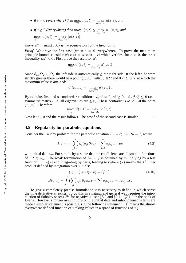
• if c = 0 (everywhere) thenmaxΩT

u(x, t) = max∂parΩT

u(x, t), and

• if c ≥ 0 (everywhere) thenmaxΩT

u(x, t) ≤ max∂parΩT

u+(x, t), and

maxΩT

|u(x, t)| = max∂parΩT

|u(x, t)| .

whereu+ = maxu, 0 is the positive part of the functionu.

Proof We prove the first case (whenc = 0 everywhere). To prove the maximumprinciple bound, consideruǫ(x, t) = u(x, t) − ǫt which verifies, forǫ > 0, the strictinequalityLuǫ < 0 . First prove the result foruǫ:

maxΩT

uǫ(x, t) = max∂parΩT

uǫ(x, t)

Since∂parΩT ⊂ ΩT the left side is automatically≥ the right side. If the left side werestrictly greater there would be a point(x∗, t∗) with x∗ ∈ Ω and0 < t∗ ≤ T at which themaximum value is attained:

uǫ(x∗, t∗) = max(x,t)∈ΩT

uǫ(x, t) .

By calculus first and second order conditions:∂juǫ = 0, uǫ

t ≥ 0 and∂2iju

ǫx ≤ 0 (as a

symmetric matrix - i.e. all eigenvalues are≤ 0). These contradictLuǫ < 0 at the point(x∗, t∗). Therefore

maxΩT

uǫ(x, t) = max∂parΩT

uǫ(x, t) .

Now let ǫ ↓ 0 and the result follows. The proof of the second case is similar. 2

4.5 Regularity for parabolic equationsConsider the Cauchy problem for the parabolic equationLu = ∂tu + Pu = f , where

Pu = −n∑

j,k=1

∂j(ajk∂ku) +n∑

j=1

bj∂ju + cu (4.9)

with initial datau0. For simplicity assume that the coefficients are all smooth functionsof x, t ∈ Ω∞. The weak formulation ofLu = f is obtained by multiplying by a testfunctionv = v(x) and integrating by parts, leading to (where( · ) means theL2 innerproduct defined by integration overx ∈ Ω):

(ut , v ) + B(u, v) = (f, v) , (4.10)

B(u, v) =

∫ (∑

jk

ajk ∂ju∂kv +∑

bj∂juv + cuv)dx .

To give a completely precise formulation it is necessary to define in which sensethe time derivativeut exists. To do this in a natural and general way requires the intro-duction of Sobolev spacesHs for negatives - see§5.9 and§7.1.1-§7.1.2 in the book ofEvans. However stronger assumptions on the initial data andinhomogeneous term aremade a simpler statement is possible. (In the following statementu(t) means the almosteverywhere defined function oft taking values in a space of functions ofx.)

5

Cop

yrig

ht ©

201

4 U

nive

rsity

of C

ambr

idge

. Not

to b

e qu

oted

or

repr

oduc

ed w

ithou

t per

mis

sion

.

Theorem 4.5.1 For u0 ∈ H10 (Ω) andf ∈ L2(ΩT ) there exists

u ∈ L2([0, T ]; H2(Ω) ∩ L∞([0, T ]; H10 (Ω))

with time derivativeut ∈ L2(ΩT ) which satisfies(4.10) for all v ∈ H10 (Ω) and almost

everyt ∈ [0, T ] and limt→0+ ‖u(t) − u0‖L2 = 0. Furthermore it is unique and has theparabolic regularityproperty:

∫ T

0

(‖u(t)‖2H2(Ω)+‖ut‖L2(Ω) ) dt+ess sup

0≤t≤T

‖u(t)‖2H1

0(Ω) ≤ C(‖f‖L2(ΩT )+‖u0‖H1

0(Ω)) .

(4.11)

The time derivative is here to be understood in a weak/distributional sense as discussedin the sections of Evans’ book just referenced, and the proofof the regularity (4.11) is in§7.1.3 of the same book. In the following result we will just verify that the bound holdsfor smooth solutions of the inhomogeneous heat equation on aperiodic interval:

Theorem 4.5.2 The Cauchy problem

ut − uxx = f , u(x, 0) = u0(x)

wheref = f(x, t) is a smooth function which is2π-periodic inx, and the initial valueu0 is also smooth and2π-periodic, admits a smooth solution fort > 0, 2π-periodic inx, which verifies the parabolic regularity estimate:

∫ T

0

( ‖ut(t)‖2L2 + ‖u(t)‖2

H2 ) dt ≤ C ( ‖u0‖2H1 +

∫ T

0

∫ π

−π

|f(x, t)|2 dxdt ) .

Here the norms inside the time integral are the Sobolev normson2π-periodic functionsof x taken at fixed time.

Proof To prove existence, search for a solution in Fourier form,u =∑

u(m, t)eimx

and obtain the ODE

∂tu(m, t) + m2u(m, t) = f(m, t) , u(m, 0) = u0(m)

which has solution

u(m, t) = e−m2tu0(m) +

∫ t

0

e−m2(t−s)f(m, s) ds .

Now by properties of Fourier series,u0(m) is a rapidly decreasing sequence, and thesame is true forf(m, t) locally uniformly in time, since

max0≤t≤T

mj|f(m, t)| ≤ 1

2π

∫ π

−π

max0≤t≤T

|∂jxf(x, t)| dx .

Now, estimatingu(m, t) for 0 ≤ t ≤ T simply as

|u(m, t)| ≤ |u0(m)| + |T | max0≤t≤T

|f(m, t)| ,

6

Cop

yrig

ht ©

201

4 U

nive

rsity

of C

ambr

idge

. Not

to b

e qu

oted

or

repr

oduc

ed w

ithou

t per

mis

sion

.

we see thatu(m, t) is a rapidly decreasing sequence sinceu0(m) andf(m, t) are. Differ-entiation in time just gives factors ofm2, and so∂j

t u(m, t) is also rapidly decreasing foreachj ∈ N . Thereforeu =

∑u(m, t)eimx defines a smooth function for positive time,

and it verifies the equation (by differentiation through thesum, since this is allowed byrapidly decreasing property just established.)

To obtain the estimate, we switch to energy methods: multiply the equation byut

and integrate. This leads to

∫ T

0

∫ π

−π

u2t dxdt +

∫ π

−π

u2x dx

∣∣t=T

=

∫ π

−π

u2x dx

∣∣t=0

+

∫ T

0

∫ π

−π

fut dxdt .

Using the Holder inequality on the final term, this gives an estimate

∫ T

0

‖ut(t)‖2L2 dt + max

0≤t≤T‖u(t)‖2

H1 ≤ C(‖u0‖2

H1 +

∫ T

0

∫ π

−π

|f(x, t)|2 dxdt)

.

(Here and belowC > 0 is just a positive constant whose precise value is not important).To obtain the full parabolic regularity estimate from this,it is only necessary to use theequation itself to estimate

∫ T

0

‖uxx(t)‖2L2 dt ≤ C

(∫ T

0

‖ut(t)‖2L2 dt +

∫ T

0

‖f(x, t)‖2L2 dt

),

and combining this with the previous bound completes the proof. 2

The parabolic regularity estimate in this theorem can alternatively be derived fromthe Fourier form of the solution (exercise).

5 Hyperbolic equations

A second order equation of the form

utt +∑

j

αj∂t∂ju + Pu = 0

with P as in (4.1) (with coefficients potentially depending upon t and x), is strictly hy-perbolic if the principal symbol

σ(τ, ξ; t, x) = −τ 2 − (α · ξ)τ +∑

jk

ajkξjξk

considered as a polynomial inτ has two distinct real rootsτ = τ±(ξ; t, x) for all nonzeroξ. We will mostly study the wave equation

utt − ∆u = 0 , (5.12)

starting with some representations of the solution for the wave equation. In this sectionwe writeu = u(t, x), rather thanu(x, t), for functions of space and time to fit in withthe most common convention for the wave equation.

7

Cop

yrig

ht ©

201

4 U

nive

rsity

of C

ambr

idge

. Not

to b

e qu

oted

or

repr

oduc

ed w

ithou

t per

mis

sion

.

5.1 The one dimensional wave equation: general solutionIntroducing characteristic coordinatesX± = x ± t, the wave equation takes the form∂2

X+X−

u = 0, which has general classical solutionF (X−) + G(X+), for arbitraryC2

functionsF,G (by calculus). Therefore, the generalC2 solution ofutt − uxx = 0 is

u(t, x) = F (x − t) + G(x + t)

for arbitraryC2 functionsF,G. (This can be proved by changing to the characteristiccoordinatesX± = x ± t , in terms of which the wave equation is∂2u

∂X+∂X−

= 0.From this can be derived the solution at timet > 0 of the inhomogeneous initial

value problem:utt − uxx = f (5.13)

with initial datau(0, x) = u0(x) , ut(0, x) = u1(x) . (5.14)

u(t, x) =1

2

(u0(x− t)+u0(x+ t)

)+

1

2

∫ x+t

x−t

u1(y) dy +1

2

∫ t

0

∫ x+t−s

x−t+s

f(s, y) dyds .

(5.15)Notice that there is again a “Duhamel principle” for the effect of the inhomogeneous

term since1

2

∫ t

0

∫ x+t−s

x−t+s

f(s, y) dyds =

∫ t

0

U(t, s, x)ds

whereU(t, s, x) is the solution of thehomogeneousproblem with dataU(s, s, x) = 0and∂tU(s, s, x) = f(s, x) specified att = s.

Theorem 5.1.1 Assuming that(u0, u1) ∈ C2(R) × C1(R) and thatf ∈ C1(R × R) theformula(5.14)defines aC2(R × R) solution of the wave equation, and furthermore foreach fixed timet, the mapping

Cr × Cr−1 → Cr × Cr−1

(u0(·), u1(·)) 7→ (u(t, ·), ut(t, ·))

is continuous for each integerr ≥ 2 . (Well-posedness inCr × Cr−1.)

The final property stated in the theorem does not hold in more than one space dimension(question 7). This is the reason Sobolev spaces are more appropriate for the higherdimensional wave equation.

5.2 The one dimensional wave equation on an interval

Next consider the problemx ∈ [0, 1] with Dirichlet boundary conditionsu(t, 0) =0 = u(t, 1). Introduce the Sturm-Liouville operatorPf = −f ′′, with these boundaryconditions as in§4.1, its eigenfunctions beingφm =

√2 sin mπx with eigenvaluesλm =

(mπ)2. In terms ofP the wave equation is:

utt + Pu = 0

8

Cop

yrig

ht ©

201

4 U

nive

rsity

of C

ambr

idge

. Not

to b

e qu

oted

or

repr

oduc

ed w

ithou

t per

mis

sion

.

and the solution with initial data

u(0, x) = u0(x) =∑

u0(m)φm , ut(0, x) = u1(x) =∑

u1(m)φm ,

is given by

u(t, x) =∞∑

m=1

cos(t√

λm)u0(m)φm +sin(t

√λm)√

λm

u1(m)φm

with an analogous formula forut. Recall the definition of the Hilbert spaceH10 ((0, 1)) as

the closure of the functions inC∞0 ((0, 1))1 with respect to the norm given by‖f‖2

H1 =∫ 1

0f 2 + f ′2 dx. In terms of the basisφm the definition is:

H10 ((0, 1)) = f =

∑fmφm : ‖f‖2

H1 =∞∑

m=1

(1 + m2π2)|fm|2 < ∞ .

(In all these expressions∑

means∑∞

m=1.) As equivalent norm we can take∑

λm|fm|2.An appropriate Hilbert space for the wave equation with these boundary conditions is tosolve for(u, ut) ∈ X whereX = H1

0 ⊕ L2, and precisely we will take the following:

X = (f, g) = (∑

fmφm,∑

gmφm) : ‖(f, g)‖2X =

∑(λm|fm|2 + |gm|2) < ∞ .

Now the effect of the evolution on the coefficientsu(m, t) andut(m, t) is the map

(u(m, t)ut(m, t)

)7→

(cos(t

√λm) sin(t

√λm)√

λm

−√

λmsin(t√

λm) cos(t√

λm)

)(u(m, 0)ut(m, 0)

)(5.16)

Theorem 5.2.1 The solution operator for the wave equation

S(t) :

(u0

u1

)7→

(u(t, ·)ut(t, ·)

)

defined by(5.16)defines a strongly continuousgroupof unitary operators on the HilbertspaceX, as in definition 6.3.1.

5.3 The wave equation onRn

To solve the wave equation onRn take the Fourier transform in the space variables toshow that the solution is given by

u(t, x) = (2π)−n

∫expiξ·x(cos(t‖ξ‖)u0(ξ) +

sin(t‖ξ‖)‖ξ‖ u1(ξ))dξ (5.17)

1i.e. smooth functions which are zero outside of a closed set[a, b] ⊂ (0, 1)

9

Cop

yrig

ht ©

201

4 U

nive

rsity

of C

ambr

idge

. Not

to b

e qu

oted

or

repr

oduc

ed w

ithou

t per

mis

sion

.

for initial valuesu(0, x) = u0(x), ut(0, x) = u1(x) in S(Rn). The Kirchhoff formulaarises from some further manipulations with the fourier transform in the casen = 3 andu0 = 0 and gives the following formula

u(t, x) =1

4πt

∫

y:‖y−x‖=t

u1(y) dΣ(y) (5.18)

for the solution at timet > 0 of utt − ∆u = 0 with initial data(u, ut) = (0, u1). Thesolution for the inhomogeneous initial value problem with general Schwartz initial datau0, u1 can then be derived from the Duhamel principle, which takes the same form as inone space dimension (as explained in§5.1).

5.4 The energy identity and finite propagation speed

Lemma 5.4.1 (Energy identity) If u is aC2 solution of the wave equation(5.12), then

∂t

(u2t + |∇u|2

2

)+ ∂i

(−ut∂iu

)= 0

where∂i = ∂∂xi .

From this and the divergence theorem some important properties follow:

Theorem 5.4.2 (Finite speed of propagation)If u ∈ C2 solves the wave equation(5.12),and if u(0, x) and ut(0, x) both vanish for‖x − x0‖ < R, thenu(t, x) vanishes for‖x − x0‖ < R − |t| if |t| < R.

Proof Notice that the energy identity can be written divt,x(e, p) = 0, where

(e, p) =(u2

t + |∇u|22

,−ut∂1u, · · · − ut∂nu)∈ R

1+n .

Let t0 > 0 and consider the backwards light cone with vertex(t0, x0), i.e. the set

(t, x) ∈ R1+3 : t ≤ t0, ‖x − x0‖ ≤ t0 − t .

The outwards normal to this at(t, x) is ν = 1√2(1, x−x0

‖x−x0‖) ∈ R1+n, which satisfies

ν · (e, p) ≥ 0 by the Cauchy-Schwarz inequality. Integrating the energy identity over theregion formed by intersecting the backwards light cone withthe slab(t, x) ∈ R

1+3 :0 ≤ t ≤ t1 , and using the divergence theorem then leads to

∫‖x−x0‖≤t0−t1

e(t1, x) dx ≤∫‖x−x0‖≤t0

e(0, x) dx . This implies the result by choosingR = t0 . 2

Theorem 5.4.3 (Regularity for the wave equation)For initial data u(0, x) = u0(x)andut(0, x) = u1(x) in S(Rn), the formula(5.17)defines a smooth solution of the waveequation(5.12), which satisfies the energy conservation law

1

2

∫

Rn

ut(t, x)2 + ‖∇u(t, x)‖2 dx = E = constant .

10

Cop

yrig

ht ©

201

4 U

nive

rsity

of C

ambr

idge

. Not

to b

e qu

oted

or

repr

oduc

ed w

ithou

t per

mis

sion

.

Furthermore, at each fixed timet there holds:

‖(u(t, ·), ut(t, ·))‖Hs+1×Hs ≤ C‖(u0(·), u1(·))‖Hs+1×Hs , C > 0 (5.19)

for eachs ∈ Z+ . Thus the wave equation is well-posed in the Sobolev normsHs+1×Hs

and regularity is preserved when measured in the SobolevL2 sense.

Proof The fact that (5.17) defines a smooth function is a consequence of the theoremson the properties of the Fourier transform and on differentiation through the integralin §2, which is allowed by the assumption that the initial data are Schwartz functions.Given this, it is straightforward to check that (5.17) defines a solution to the wave equa-tion. Energy conservation follows by integrating the identity in lemma 5.4.1. Energyconservation almost gives (5.19) fors = 0. It is only necessary to bound‖u(t, ·)‖2

L2 ,which may be done in the following way. To start, using energyconservation, we have:

∣∣ d

dt‖u‖2

L2

∣∣ =∣∣ 2(u, ut)L2

∣∣ ≤ ‖u‖L2‖ut‖L2 ≤√

2E‖u‖L2

This implies thatFǫ(t) = (ǫ + ‖u(t, ·)‖2L2)

1

2 satisfies2, for any positiveǫ

Fǫ(t) ≤√

2E

and hence‖u(t, ·)‖L2 ≤ Fǫ(t) ≤ (ǫ + ‖u(0, ·)‖2L2)

1

2 +√

2Et, for any ǫ > 0. Thiscompletes the derivation of (5.19) fors = 0 . The corresponding cases of (5.19) fors = 1, 2 . . . are then derived by successively differentiating the equation, and applyingthe energy conservation law to the differentiated equation. 2

Remark 5.4.4 Well-posedness and preservation of regularity do not hold for the waveequation when measured in uniform normsCr × Cr−1, except in one space dimension,see question 7.

Remark 5.4.5 For initial data (u0, u1) ∈ Hs+1 × Hs there is a distributional solution(u(t, ·), ut(t, ·)) ∈ Hs+1 × Hs at each time, which can be obtained by approximationusing density ofC∞

0 in the Sobolev spacesHs and the well-posedness estimate(5.19).

6 One-parameter semigroups and groups

If A is a bounded linear operator on a Banach space its norm is

‖A‖ = supu∈X,u 6=0

‖Au‖‖u‖ , (operator or uniform norm).

This definition implies that ifA,B are bounded linear operators onX then‖AB‖ ≤‖A‖‖B‖ .

2Theǫ is introduced to avoid the possibility of dividing by zero.

11

Cop

yrig

ht ©

201

4 U

nive

rsity

of C

ambr

idge

. Not

to b

e qu

oted

or

repr

oduc

ed w

ithou

t per

mis

sion

.

6.1 DefinitionsDefinition 6.1.1 A one-parameter family of bounded linear operatorsS(t)t≥0 on aBanach spaceX forms a semigroup if

1. S(0) = I (the identity operator) , and

2. S(t + s) = S(t)S(s) for all t, s ≥ 0 (semi-group property).

3. It is called a uniformly continuous semigroup if in addition to (1) and (2):

limt→0+

‖S(t) − I‖ = 0 , (uniform continuity).

4. It is called a strongly continuous (orC0) semigroup if in addition to (1) and (2):

limt→0+

‖S(t)u − u‖ = 0 ,∀u ∈ X (strong pointwise continuity).

5. If ‖S(t)‖ ≤ 1 for all t ≥ 0 the semigroupS(t)t≥0 is called a semigroup ofcontractions.

Notice that in 3 the symbol‖ · ‖ means the operator norm, while in 4 the same symbolmeans the norm on vectors inX. Also observe that uniform continuity is a strongercondition than strong continuity.

6.2 Semigroups and their generatorsFor ordinary differential equationsx = Ax, whereA is ann×n matrix, the solution canbe writtenx(t) = etAx(0) and there is a1− 1 corespondence between the matrixA andthe semigroupS(t) = etA on R

n. In this subsection3 we discuss how this generalizes.Uniformly continuous semigroups have a simple structure which generalizes the fi-

nite dimensional case in an obvious way - they arise as solution operators for differentialequations in the Banach spaceX:

du

dt+ Au = 0 , for u(0) ∈ X given. (6.20)

Theorem 6.2.1 S(t)t≥0 is a uniformly continuous semgroup onX if and only if thereexists a unique bounded linear operatorA : X → X such thatS(t) = e−tA =∑∞

j=0(−tA)j/j!. This semigroup gives the solution to(6.20)in the formu(t) = S(t)u(0),which is continuously differentiable intoX. The operatorA is called the infinitesimalgenerator of the semigroupS(t)t≥0.

This applies to ordinary differential equations whenA is a matrix. It is not very usefulfor partial differential equations because partial differential operators are unbounded,whereas in the foregoing theorem the infinitesimal generator was necessarily bounded.For example for the heat equation we need to takeA = −∆, the laplacian defined onsome appropriate Banach space of functions. Thus it is necessary to consider moregeneral semigroups, in particular the strongly continuoussemigroups. An unboundedlinear operatorA is a linear map from a linear subspaceD(A) ⊂ X into X (or moregenerally into another Banach spaceY ). The subspaceD(A) is called the domain ofA.An unbounded linear operatorA : D(A) → Y is said to be

3This subsection is for background information only

12

Cop

yrig

ht ©

201

4 U

nive

rsity

of C

ambr

idge

. Not

to b

e qu

oted

or

repr

oduc

ed w

ithou

t per

mis

sion

.

• densely definedif D(A) = X, where the overline means closure in the norm ofX, and

• closedif the graphΓA = (u,Au)|u∈D(A) ⊂ X × Y is closed inX × Y .

A class of unbounded linear operators suitable for understanding strongly continuoussemigroups is the class ofmaximal monotoneoperators in a Hilbert space:

Definition 6.2.2 1. A linear operatorA : D(A) → X on a Hilbert spaceX ismonotone if(u,Au) ≥ 0 for all u ∈ D(A).

2. A monotone operatorA : D(A) → X is maximal monotone if, in addition, therange ofI + A is all of X, i.e. if:

∀f ∈ X ∃u ∈ D(A) : (I + A)u = f .

Maximal monotone operators are automatically densely defined and closed, and there isthe following generalization of theorem 6.2.1:

Theorem 6.2.3 (Hille-Yosida) If A : D(A) → X is maximal monotone then the equa-tion

du

dt+ Au = 0 , for u(0) ∈ D(A) ⊂ X given, (6.21)

admits a unique solutionu ∈ C([0,∞); D(A)) ∩ C1([0,∞); X) with the property that‖u(t)‖ ≤ ‖u(0)‖ for all t ≥ 0 and u(0) ∈ D(A). SinceD(A) ⊂ X is dense themapD(A) ∋ u(0) → u(t) ∈ X extends to a linear mapSA(t) : X → X and byuniqueness this determines a strongly continuous semigroup of contractionsSA(t)t≥0

on the Hilbert spaceX. OftenSA(t) is written asSA(t) = e−tA.Conversely, given a strongly continuous semigroupS(t)t≥0 of contractions onX,

there exists a unique maximal monotone operatorA : D(A) → X such thatSA(t) =S(t) for all t ≥ 0. The operatorA is the infinitesimal generator ofS(t)t≥0 in thesense thatd

dtS(t)u = Au for u ∈ D(A) andt ≥ 0 (interpreting the derivative as a right

derivative att = 0).

6.3 Unitary groups and their generatorsSemigroups arise in equations which are not necessarily time reversible. For equationswhich are, e.g. the Schrodinger and wave equations, each time evolution operator has aninverse and the semigroup is in fact a group. In this subsection4 We give the definitionsand state the main result.

Definition 6.3.1 A one-parameter family of unitary operatorsU(t)t∈R on a HilbertspaceX forms a group of unitary operators if

1. U(0) = I (the identity operator) , and

2. U(t + s) = U(t)U(s) for all t, s ∈ R (group property).

4In this subsection you only need to know definition 6.3.1. Theremainder is for background informa-tion.

13

Cop

yrig

ht ©

201

4 U

nive

rsity

of C

ambr

idge

. Not

to b

e qu

oted

or

repr

oduc

ed w

ithou

t per

mis

sion

.

3. It is called a strongly continuous (orC0) group of unitary operators if in additionto (1) and (2):

limt→0

‖U(t)u − u‖ = 0 ,∀u ∈ X (strong pointwise continuity).

A maximal monotone operatorA which is symmetric (=hermitian), i.e. such that

(Au, v) = (u,Av) for all u, v in D(A) ⊂ X (6.22)

generates a one-parametergroupof unitary operatorsU(t)t∈R, often writtenU(t) =e−itA, by solving the equation

du

dt+ iAu = 0 , for u(0) ∈ D(A) ⊂ X given. (6.23)

It is useful to introduce the adjoint operatorA∗ via the Riesz representation theorem:first of all let

D(A∗) = u ∈ X : the mapv 7→ (u,Av) extends to a

bounded linear functionalX → C

so thatD(A∗) is a linear space, and foru ∈ D(A∗) there exists a vectorwu such that(wu, v) = (u,Av) (by Riesz representation). The mapu → wu is linear onD(A∗)and so we can define an unbounded linear operatorA∗ : D(A∗) → X by A∗u = wu,and since we started with a symmetric operator it is clear that D(A) ⊂ D(A∗) andA∗u = Au for u ∈ D(A); the operatorA∗ is thus an extension ofA.

Definition 6.3.2 If A : D(A) → X is an unbounded linear operator which is symmetricand ifD(A∗) = D(A) thenA is said to be self-adjoint and we writeA = A∗.

Theorem 6.3.3 Maximal monotone symmetric operators are self-adjoint.

Theorem 6.3.4 (Stone theorem)If A is a self-adjoint operator the equation(6.23)hasa unique solution foru(0) ∈ D(A) which may be writtenu(t) = UA(t)u(0) with‖u(t)‖ = ‖u(0‖ for all t ∈ R. It follows that theUA(t) extend uniquely to defineunitary operatorsX → X and thatUA(t)t∈R constitutes a strongly continuous groupof unitary operators which are writtenUA(t) = e−itA.

Conversely, given a strongly continuous group of unitary operatorsU(t)t∈R thereexists a self-adjoint operatorA such thatU(t) = UA(t) = e−itA for all t ∈ R.

6.4 Worked problems1. LetC∞

per = u ∈ C∞(R) : u(x + 2π) = u(x) be the space of smooth2π− periodic functionsof one variable.

(i) For f ∈ C∞per show that there exists a uniqueu = uf ∈ C∞

per such that

−∂2u

∂x2+ u = f.

14

Cop

yrig

ht ©

201

4 U

nive

rsity

of C

ambr

idge

. Not

to b

e qu

oted

or

repr

oduc

ed w

ithou

t per

mis

sion

.

(ii) Show thatIf [uf + φ] > If [uf ] for every φ ∈ C∞per which is not identically zero, where

If : C∞per → R is defined by

If [u] =1

2

∫ +π

−π

((∂u

∂x)2 + u2 − 2f(x)u

)dx.

(iii) Show that the equation∂u

∂t− ∂2u

∂x2+ u = f(x),

with initial datau(0, x) = u0(x) ∈ C∞per has, fort > 0 a smooth solutionu(t, x) such that

u(t, ·) ∈ C∞per for each fixedt > 0, and give a representation of this solution as a Fourier series in

x. Calculatelimt→+∞ u(t, x) and comment on your answer in relation to (i).

(iv) Show thatIf [u(t, ·)] ≤ If [u(s, ·)] for t > s > 0, and thatIf [u(t, ·)] → If [uf ] ast → +∞.

Answer(i) Any solutionuf ∈ C∞per can be represented as a Fourier series:uf =

∑uf (α)eiαx, as

canf . Hereα ∈ Z. The fourier coefficients are rapidly decreasing i.e. faster than any polynomialso it is permissible to differentiate through the sum, and substituting into the equation we find thatthe coefficientsuf (α) are uniquely determined byf according to(1 + α2)uf (α) = f(α), hence

uf (x) =∑ f(α)

1 + α2eiαx.

(Can also prove uniqueness by noting that if there were two solutionsu1, u2 then the differenceu = u1 − u2 would solve−uxx + u = 0. Now multply byu and integrating by parts (usingperiodicity) - this implies that

∫u2

x + u2 = 0 which implies thatu = u1 − u2 = 0.)

(ii) Calculate, using the equation satisfied byuf and integration by parts, that

If [uf + φ] − If [uf ] =1

2

∫ π

π

(φ2x + φ2)dx > 0

for non-zeroφ ∈ C∞per.

(iii) Expand the solution in terms of Fourier series and thensubstitute into the equation and useintegrating factor to obtain that the solution isu(t, x) =

∑u(α, t)eiαx where

u(α, t) = e−t(1+α2)u0(α) +

∫ t

0

e−(t−s)(1+α2)f(α)ds.

Carry out the integral to deduce that

u(α, t) =f(α)

1 + α2+ e−t(1+α2)

(u0(α) − f(α)

1 + α2

).

which implies thatu(α, t) → uf (α) = f(α)1+α2 as t → +∞, and further thatu(x, t) → uf (x)

uniformly in x ast → +∞.

(iv) By (i) and (iii) we see thatu(x, t) = uf (x) + φ(x, t) whereφ(α, t) = e−t(1+α2)(u0(α) −uf (α)). Now apply (ii) and use the Parseval theorem to deduce that

If [u(t, ·)] − If [uf ] = π∑

(1 + α2)|φ(α, t)|2

= π∑

(1 + α2)e−2t(1+α2)|u0(α) − uf (α)|2

which decreases to zero sinceu0(α) anduf (α) are rapidly decreasing.

15

Cop

yrig

ht ©

201

4 U

nive

rsity

of C

ambr

idge

. Not

to b

e qu

oted

or

repr

oduc

ed w

ithou

t per

mis

sion

.

2. For the equationut − uxx + u = f , wheref = f(x, t) is a smooth function which is2π-periodicin x, and the initial datau(x, 0) = u0(x) are also smooth and2π-periodic obtain the solution as aFourier seriesu =

∑u(m, t)eimx and hence verify the parabolic regularity estimate:

∫ T

0

( ‖ut(t)‖2L2 + ‖u(t)‖2

H2 ) dt ≤ C ( ‖u0‖2H1 +

∫ T

0

∫ π

−π

|f(x, t)|2 dxdt ) .

Answer:Use the Fourier form of the solutionu(x, t) =∑

m∈Zn u(m, t)eim·x at each timet, andsimilarly for f , and the definition

Hsper = u =

∑

m∈Zn

u(m)eim·x ∈ L2 : ‖u‖2Hs =

∑

m∈Zn

(1 + ‖m‖2)s|u(m)|2 < ∞ ,

is for the Sobolev spaces of fixed time functions2π-periodic in each co-ordinatexj and fors =0, 1, 2, . . . . Writing ωm = 1 + ‖m‖2, and using an integrating factor the solution is given by:

u(m, t) = e−ωmtu(m, 0) +

∫ t

0

e−(t−s)ωm f(m, s) ds

in Fourier representation. The second term is a convolution, so by the Hausdorff-Young inequality‖f ∗ g‖2

L2 ≤ ‖f‖2L1‖g‖2

L2 we obtain:

∫ T

0

|∫ t

0

e−(t−s)ωm f(m, s) ds |2 dt ≤(∫ T

0

|e−tωm |dt)2

∫ T

0

|f(m, t)|2dt

≤ 1

ω2m

∫ T

0

|f(m, t)|2dt .

Here we have made use of∫ T

0e−ωmt dt = 1−e−ωmT

ωm≤ 1

ωm. Using this bound, and|a + b|2 ≤

2(a2 + b2), we obtain:

∫ T

0

ω2m|u(m, t)|2 dt ≤ 2

[∫ T

0

e−2tωm dt ω2m |u(m, 0)|2 +

∫ T

0

|f(m, t)|2dt]

≤ 2[ ωm

2|u(m, 0)|2 +

∫ T

0

|f(m, t)|2dt].

Now sum overm ∈ Zn and use the Parseval theorem and definitions of‖ · ‖Hs to obtain

∫ T

0

‖u(t)‖2H2 dt ≤ const.

[‖u(0)‖2

H1 +

∫ T

0

|f(t)|2L2 dt].

To obtain the inequality as stated it is sufficient to use the equation to obtain the same bound for∫ T

0‖ut(t)‖2

L2 dt (with another constant).

3. (i) Define the Fourier transformf = F(f) of a Schwartz functionf ∈ S(Rn), and also of atempered distributionu ∈ S ′(Rn).

(ii) From your definition compute the Fourier transform of the distributionWt ∈ S ′(R3) given by

Wt(ψ) =< Wt, ψ >=1

4πt

∫

‖y‖=t

ψ(y)dΣ(y)

16

Cop

yrig

ht ©

201

4 U

nive

rsity

of C

ambr

idge

. Not

to b

e qu

oted

or

repr

oduc

ed w

ithou

t per

mis

sion

.

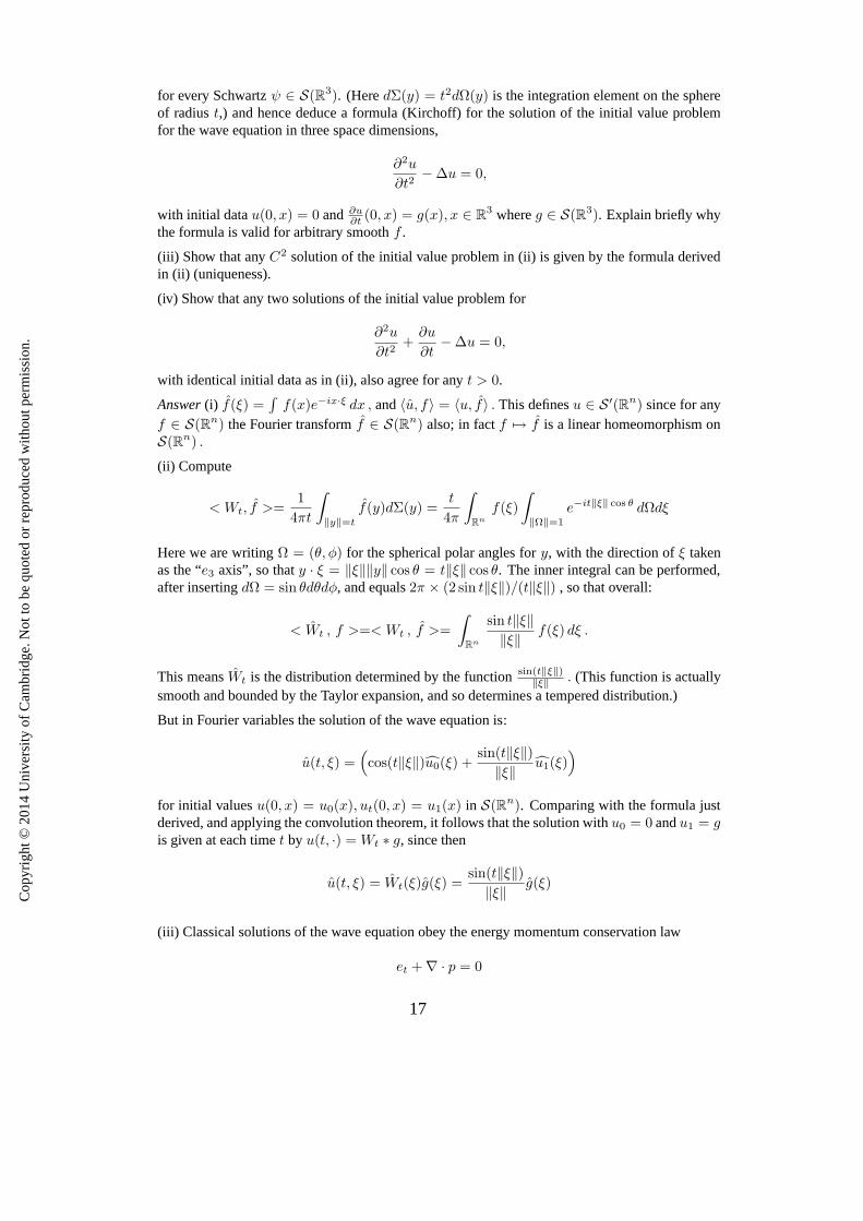
for every Schwartzψ ∈ S(R3). (HeredΣ(y) = t2dΩ(y) is the integration element on the sphereof radiust,) and hence deduce a formula (Kirchoff) for the solution of the initial value problemfor the wave equation in three space dimensions,

∂2u

∂t2− ∆u = 0,

with initial datau(0, x) = 0 and ∂u∂t (0, x) = g(x), x ∈ R

3 whereg ∈ S(R3). Explain briefly whythe formula is valid for arbitrary smoothf .

(iii) Show that anyC2 solution of the initial value problem in (ii) is given by the formula derivedin (ii) (uniqueness).

(iv) Show that any two solutions of the initial value problemfor

∂2u

∂t2+

∂u

∂t− ∆u = 0,

with identical initial data as in (ii), also agree for anyt > 0.

Answer(i) f(ξ) =∫

f(x)e−ix·ξ dx , and〈u, f〉 = 〈u, f〉 . This definesu ∈ S ′(Rn) since for anyf ∈ S(Rn) the Fourier transformf ∈ S(Rn) also; in factf 7→ f is a linear homeomorphism onS(Rn) .

(ii) Compute

< Wt, f >=1

4πt

∫

‖y‖=t

f(y)dΣ(y) =t

4π

∫

Rn

f(ξ)

∫

‖Ω‖=1

e−it‖ξ‖ cos θ dΩdξ

Here we are writingΩ = (θ, φ) for the spherical polar angles fory, with the direction ofξ takenas the “e3 axis”, so thaty · ξ = ‖ξ‖‖y‖ cos θ = t‖ξ‖ cos θ. The inner integral can be performed,after insertingdΩ = sin θdθdφ, and equals2π × (2 sin t‖ξ‖)/(t‖ξ‖) , so that overall:

< Wt , f >=< Wt , f >=

∫

Rn

sin t‖ξ‖‖ξ‖ f(ξ) dξ .

This meansWt is the distribution determined by the functionsin(t‖ξ‖)‖ξ‖ . (This function is actually

smooth and bounded by the Taylor expansion, and so determines a tempered distribution.)

But in Fourier variables the solution of the wave equation is:

u(t, ξ) =(cos(t‖ξ‖)u0(ξ) +

sin(t‖ξ‖)‖ξ‖ u1(ξ)

)

for initial valuesu(0, x) = u0(x), ut(0, x) = u1(x) in S(Rn). Comparing with the formula justderived, and applying the convolution theorem, it follows that the solution withu0 = 0 andu1 = gis given at each timet by u(t, ·) = Wt ∗ g, since then

u(t, ξ) = Wt(ξ)g(ξ) =sin(t‖ξ‖)

‖ξ‖ g(ξ)

(iii) Classical solutions of the wave equation obey the energy momentum conservation law

et + ∇ · p = 0

17

Cop

yrig

ht ©

201

4 U

nive

rsity

of C

ambr

idge

. Not

to b

e qu

oted

or

repr

oduc

ed w

ithou

t per

mis

sion

.

wheree = (u2t + |∇u|2)/2 andp = −ut∇u. Integrateet + ∇ · p = 0 over the part of the

backward light cone with vertex(t0, x0), for somet0 > 0 , which lies in the slab betweent = 0andt = t1 < t0; i.e. the region

Kt0,x0= (t, x) ∈ R

1+3 : 0 ≤ t ≤ t1, ‖x − x0‖ ≤ t0 − t .

Applying the divergence theorem, and noticing that ifν is the outward pointing normal on thesloping part of the boundary of this region, thenν · (e, p) ≥ 0 by the Cauchy-Schwarz inequality,we deduce that ∫

‖x−x0‖≤t0−t1

e(t1, x) dx ≤∫

‖x−x0‖≤t0

e(0, x) dx . (6.24)

This implies that if the initial data are zero then the solution is zero at all later times. By timereversal symmetry an identical argument implies the same thing for negative times. Applied tothe difference of two solutions this implies uniqueness (since by linearity the difference of twosolutions of the wave equation also solves the wave equation), and hence that any classicalC2

solution is given by the same formula as was derived in (ii).

(iv) Do essentially the same calculation as in (iii) but using this time that

et + ∇ · p = −u2t ≤ 0

which gives the same conclusion 6.24 for positive times. (However, since time reversal symmetryno longer holds, the argument cannot now be simply reversed to obtain the analogous inequalityfor negative times).

4. Consider acontinuousfunctiont 7→ u(t) ∈ C such that|u(t)| = 1∀t andu(t + s) = u(t)u(s) forall reals, t . Prove that there existsa ∈ R such thatu(t) = eiat. Deduce Stone’s theorem on theHilbert spaceC .

AnswerThere existsλ(t), defined mod2π, such thatu(t) = eiλ(t). By continuity there existsδ > 0 such that for|t| ∈ I = (−δ,+δ) we have|u(t)−1| < 1

2 . In this intervalI, there is a uniqueλ(t) ∈ (−π,+π) which is continuous and satisfiesu(t) = eiλ(t) andλ(t + s) = λ(t) + λ(s) fors, t, s+t all in I. LetN be any integer sufficiently large that1N ∈ I, and definea = Nλ( 1

N ). Then

the semigroup property implies thatu(mN ) = (u( 1

N ))m = eimλ( 1N

) = eia mN , for any integerm.

The value ofa thus defined is independent ofN chosen as above: indeed, ifa′, N ′ were anothersuch value we would also haveu(t) = eia′ m

N′ for all integralm. Clearly 1NN ′

∈ I, so also definingb = NN ′λ( 1

NN ′) we have by the additivity ofλ thata = b = a′. Thereforea is unique, for all

such integersN with 1N ∈ I and sou(t) = eia m

N for all suchN and allm ∈ Z. It follows fromthe density ofmN in R and the continuity ofu(t) thatu(t) = eiat for all t ∈ R .

18

Cop

yrig

ht ©

201

4 U

nive

rsity

of C

ambr

idge

. Not

to b

e qu

oted

or

repr

oduc

ed w

ithou

t per

mis

sion

.

6.5 Example sheet 41. (a) Use the change of variablesv(t, x) = etu(t, x) to obtain an “x-space” formula for the solution

to the initial value problem:

ut + u = ∆u u(0, · ) = u0(·) ∈ S(Rn).

Hence show that|u(t, x)| ≤ supx |u0(x)| and use this to deduce well-posedness in the supremumnorm (fort > 0 and allx).

If a ≤ u0(x) ≤ b for all x what can you say about the possible values ofu(t, x) for t > 0.

(b) Use the Fourier transform inx to obtain a (Fourier space) formula for the solution of:

utt − 2ut + u = ∆u u(0, · ) = u0(·) ∈ S(Rn), ut(0, ·) = u1(·) ∈ S(Rn).

2. Show that ifu ∈ C([0,∞)×Rn)∩C2((0,∞)×R

n) satisfies (i) the heat equation, (ii)u(0, x) = 0and (iii) |u(t, x)| ≤ M and |∇u(t, x)| ≤ N for someM,N thenu ≡ 0. (Hint: multiply heatequation byKt0−t(x−x0) and integrate over|x| < R, a < t < b. Apply the divergence theorem,carefully letR → ∞ and thenb → t0 anda → 0 to deduceu(t0, x0) = 0.)

3. Show that ifS(t) is a strongly continuous semigroup of contractions on a Banach spaceX withnorm‖ · ‖, then

limt→0+

‖S(t0 + t)u − S(t0)u‖ = 0 , ∀u ∈ X and∀t0 > 0 .

4. LetPu = −(pu′)′ + qu, with p andq smooth, be a Sturm-Liouville operator on the unit interval[0, 1] and assume there exist constantsm, c0 such thatp ≥ m > 0 andq ≥ c0 > 0 everywhere,and consider Dirichlet boundary conditionsu(0) = 0 = u(1). Assumeφn∞n=1 are smoothfunctions which constitute an orthonormal basis forL2([0, 1]) of eigenfunctions:Pφn = λnφn.Show that there exists a numberγ > 0 such thatλn ≥ γ for all n. Write down the solution tothe equation∂tu + Pu = 0 with initial datau0 ∈ L2([0, 1]) and show that it defines a stronglycontinuous semigroup of contractions onL2([0, 1]), and describe the large time behaviour.

5. (i) Let ∂tuj + Puj = 0 , j = 1, 2 whereP is as in (4.1) and the functionsuj have the regularityassumed in theorem 4.4.1 and satisfy Dirichlet boundary conditions:uj(x, t) = 0∀x ∈ ∂Ω, t ≥ 0.Assuming, in addition to (4.2), that

c ≥ c0 > 0 (6.25)

for some positive constantc0 prove that for all0 ≤ t ≤ T :

supx∈Ω

|u1(x, t) − u2(x, t)| ≤ e−tc0 supx∈Ω

|u1(x, 0) − u2(x, 0)|.

(ii) In the situation of part (i) with

Pu = −n∑

j,k=1

∂j(ajk∂ku) +

n∑

j=1

bj∂ju + cu , (6.26)

assuming in addition to (4.2) and (6.25) also thatajk, bj areC1 and that

n∑

j=1

∂jbj = 0 , in ΩT ,

prove that for all0 ≤ t ≤ T :∫

Ω

|u1(x, t) − u2(x, t)|2 dx ≤ e−2tc0

∫

Ω

|u1(x, 0) − u2(x, 0)|2 dx.

19

Cop

yrig

ht ©

201

4 U

nive

rsity

of C

ambr

idge

. Not

to b

e qu

oted

or

repr

oduc

ed w

ithou

t per

mis

sion

.

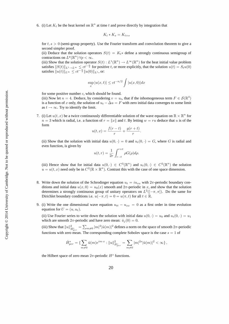
6. (i) Let Kt be the heat kernel onRn at timet and prove directly by integration that

Kt ∗ Ks = Kt+s

for t, s > 0 (semi-group property). Use the Fourier transform and convolution theorem to give asecond simpler proof.(ii) Deduce that the solution operatorsS(t) = Kt∗ define a strongly continuous semigroup ofcontractions onLp(Rn)∀p < ∞.(iii) Show that the solution operatorS(t) : L1(Rn) → L∞(Rn) for the heat initial value problemsatisfies‖S(t)‖L1→L∞ ≤ ct−

n2 for positivet, or more explicitly, that the solutionu(t) = Stu(0)

satisfies‖u(t)‖L∞ ≤ ct−n2 ‖u(0)‖L1 , or:

supx

|u(x, t)| ≤ ct−n/2

∫|u(x, 0)|dx

for some positive numberc, which should be found.(iii) Now let n = 4. Deduce, by consideringv = ut, that if the inhomogeneous termF ∈ S(R4)is a function ofx only, the solution ofut −∆u = F with zero initial data converges to some limitast → ∞. Try to identify the limit.

7. (i) Let u(t, x) be a twice continuously differentiable solution of the waveequation onR × Rn for

n = 3 which is radial, i.e. a function ofr = ‖x‖ andt. By lettingw = ru deduce thatu is of theform

u(t, x) =f(r − t)

r+

g(r + t)

r.

(ii) Show that the solution with initial datau(0, ·) = 0 andut(0, ·) = G, whereG is radial andeven function, is given by

u(t, r) =1

2r

∫ r+t

r−t

ρG(ρ)dρ.

(iii) Hence show that for initial datau(0, ·) ∈ C3(Rn) and ut(0, ·) ∈ C2(Rn) the solutionu = u(t, x) need only be inC2(R × R

n). Contrast this with the case of one space dimension.

8. Write down the solution of the Schrodinger equationut = iuxx with 2π-periodic boundary con-ditions and initial datau(x, 0) = u0(x) smooth and2π-periodic inx, and show that the solutiondetermines a strongly continuous group of unitary operators onL2([−π, π]). Do the same forDirichlet boundary conditions i.e.u(−π, t) = 0 = u(π, t) for all t ∈ R.

9. (i) Write the one dimensional wave equationutt − uxx = 0 as a first order in time evolutionequation forU = (u, ut).

(ii) Use Fourier series to write down the solution with initial datau(0, ·) = u0 andut(0, ·) = u1

which are smooth2π-periodic and have zero mean:uj(0) = 0.

(iii) Show that‖u‖2H1

per

=∑

m 6=0 |m|2|u(m)|2 defines a norm on the space of smooth2π-periodic

functions with zero mean. The corresponding complete Sobolev space is the cases = 1 of

Hsper =

∑

m 6=0

u(m)eim·x : ‖u‖2Hs

per

=∑

m 6=0

|m|2s|u(m)|2 < ∞ ,

the Hilbert space of zero mean2π-periodicHs functions.

20

Cop

yrig

ht ©

201

4 U

nive

rsity

of C

ambr

idge

. Not

to b

e qu

oted

or

repr

oduc

ed w

ithou

t per

mis

sion

.

(iv) Show that the solution defines a group of unitary operators in the Hilbert space

X = U = (u, v) : u ∈ H1per andv ∈ L2([−π, π]) .

(v) Explain the “unitary” part of your answer to (iv) in termsof the energy

E(t) =

∫ π

−π

(u2t + u2

x) dx .

(vi) Show that‖U(t)‖Hs+1per ⊕Hs

per= ‖(u0, u1)‖Hs+1

per ⊕Hsper

(preservation of regularity).

10. (a) Deduce from the finite speed of propagation result forthe wave equation (lemma 5.4.2) thata classical solution of the initial value problem,2u = 0, u(0, t) = f, ut(0, x) = g, with f, g ∈D(Rn) given is unique.

(b) The Kirchhoff formula for solutions of the wave equationn = 3 for initial datau(0, ·) =0, ut(0, ·) = g is derived using the Fourier transform wheng ∈ S(Rn). Show that the valid-ity of the formula can be extended to any smooth functiong ∈ C∞(Rn).(Hint: finite speed ofpropagation).

11. Write out and prove Stone’s theorem for the case of the finite dimensional Hilbert spaceCN (sothat each operatorU(t) is now a unitary matrix).

21