Partial Differendal Equadons inTwo Space...

(5.1)

Partial Differendal Equadons in TwoSpace Variables

INTRODUCTION

In Chapter 4 we discussed the various classifications of PDEs and describedfinite difference (FD) and finite element (FE) methods for solving parabolicPDEs in one space variable. This chapter begins by outlining the solution ofelliptic PDEs using FD and FE methods. Next, parabolic PDEs in two spacevariables are treated. The chapter is then concluded with a section on mathematical software, which includes two examples.

ELLIPTIC rOES-fiNITE DIffERENCES

Background

Let R be a bounded region in the x - y plane with boundary aR. The equation

~ [alex, y) aw] + ~ [az(x, y) aw] = d (x, y, w, aw, aw)ax ax ay ay ax ayalaz > 0

is elliptic in R (see Chapter 4 for the definition of elliptic equations), and threeproblems involving (5.1) arise depending upon the subsidiary conditions prescribed on aR:

1. Dirichlet problem:

w = f(x, y) on aR (5.2)

111

178 Partial Differential Equations in Two Space Variables

2. Neumann problem:

aw- = g(x, y) on aRan

where a/an refers to differentiation along the outward normal to aR

3. Robin problem:

awu(x, y)w + ~(x, y) an = "{(x, y) on aR

We illustrate these three problems on Laplace's equation in a square.

laplace's Equation in a Square

Laplace's equation is

(5.3)

(5.4)

o~ x ~ 1, 0 ~ Y ~ 1 (5.5)

Let the square region R, 0 ~ x ~ 1, 0 ~ y ~ 1, be covered by a grid with sidesparallel to the coordinate axis and grid spacings such that Llx = Ily = h. IfNh = 1, then the number of internal grid points is (N - 1)2. A second-orderfinite difference discretization of (5.5) at any interior node is:

1 1(IlX)2 [Ui+1,j - 2ui ,j + Ui-1,j] + (lly)2 [Ui,j+l - 2ui ,j + ui,j-d = 0 (5.6)

where

Ui,j = w(xi , y)Xi = ihYj = jh

Since Ilx = Ily, (5.6) can be written as:

Ui,j-l + Ui+1,j - 4ui ,j + Ui-1,j + Ui,j+l = 0

with an error of O(h2).

Dirichlet Problem If w = f(x, y) on aR, then

Ui,j = f(x i , Yj)

(5.7)

(5.8)

for (x;, yJ on aR. Equations (5.7) and (5.8) completely specify the discretization,and the ensuing matrix problem is

Au = f (5.9)

Elliptic PDES-Finite Differences

where

179

A

J

-[

°

-[ °

(N - 1)2 x (N - 1)2

-1

-1

1 = identity matrix,

4 -1

-1J=

J

(N - 1) x (N - 1)

(N - 1) x (N - 1)-1

-1 . 4

U = [Ul,l, ... , UN-l,l, Ul,b ... , UN-l,b ... , Ul,N-V ... , UN_l,N_d T

f = [teO, Yl) + f(xv 0), f(X2' 0), ... ,f(XN-V 0)

+ f(l, Yl), f(O, Yz), 0, ... ,0, f(l, Yz), ... ,f(O, YN-l)

+ f(xv 1), f(xv 1), f(X2' 1), ... ,f(xN-v 1) + f(l, YN-l»)T

Notice that the matrix A is block tridiagonal and that most of its elements arezero. Therefore, when solving problems of this type, a matrix-solving techniquethat takes into account the sparseness and the structure of the matrix should beused. A few of these techniques are outlined in Appendix E.

Neumann Problem Discretize (5.3) using the method of false boundaries togIVe:

or

where

gO,j = g(O, jh)

(5.10)


Combine (5.10) and (5.7) with the result

Au = 2hg (5.11)

where

K -21

-1

A= (N + 1)2 X (N + If-1

-21 K

4 -2-1 4 -1-1

K = (N + 1) x (N + 1)

-1 4-1-2 4

1 = identity matrix, (N + 1) x (N + 1)

u = [uo,o, ... , UN,O, UO,l' ... , UN,l' ... , UO,N, ... , UN,N]T

g = [2go,o, gl,O, , 2gN,o, gO,l' 0, ... , 0, gN,l' ... ,

2g0,N' gl,N, , gN-l,N, 2gN,NF

In contrast to the Dirichlet problem, the matrix A is now singular. Thus A hasonly (N + If - 1 rows or columns that are linearly independent. The solutionof (5.11) therefore involves an arbitrary constant. This is a characteristic of thesolution of a Neumann problem.

(5.12)

for 0,;:;; x,;:;; 1

for 0,;:;; y ,;:;; 1x = 01}x=

y=O}y = 1

away - <P2W = go(x),

aw- + T) w = gl(X),ay 2

Robin Problem. Consider the boundary conditions of form

awax - <hw = Jo(Y),

Elliptic PDES-Finite Differences 181

where <I> and 11 are constants and f and g are known functions. Equations (5.12)can be discretized, say by the method of false boundaries, and then included inthe discretization of (5.5). During these discretizations, it is important to maintain the same order of accuracy in the boundary discretization as with the PDEdiscretization. The resulting matrix problem will be (N + 1)2 X (N + 1)2, andits form will depend upon (5.12).

Usually, a practical problem contains a combination of the different typesof boundary conditions, and their incorporation into the discretization of thePDE can be performed as stated above for the three cases.

EXAMPLE 1

Consider a square plate Rconduction equation

{(x, y): 0 ~ x ~ 1, 0 ~ Y ~ I} with the heat

Set up the finite difference matrix problem for this equation with the followingboundary conditions:

T(x, y) = T(O, y)

T(I, y)

~; (x, 0) = 0

aT- (x, 1) = k[T(x, 1) - T2]ay

(fixed temperature)

(fixed temperature)

(insulated surface)

(heat convected away at y 1)

where Tv T2, and k are constants and T1 ~ T(x, y) ~ T2 .

SOLUTION

Impose a grid on the square region R such that Xi = ih, Yj = jh (Lix = Liy) andNh = 1. For any interior grid point

Ui,j-l + Ui+1,j - 4ui ,j + Ui-1,j + Ui,j+l = 0

where

182

y

Partial Differential Equations in Two Space Variables

0,4

0,3

0,1

aT = k(T-T: )ay 2

1,4 2,4 3,4 4,4

13 23 3.3 43

12 22 32 42T=T2

II 21 31 41

0,0 1,0 2,0

aT =0ay

3,0 4,0x

FIGURE. 5. t Grid fOil" Example t.

At the boundaries xTherefore

°and x 1 the boundary conditions are Dirichlet.

for j = 0, ... ,N

for j = 0, ... ,N

At Y = °the insulated surface gives rise to a Neumann condition that can bediscretized as

and at y

Ui,-l - Ui,l = 0,

1 the Robin condition is

for i = 1, . . . , N - 1

Ui,N-l - Ui,N+l = k[. - T]2h U"N 2 , for i = 1, . . . , N - 1

If N = 4, then the grid is as shown inFigure 5.1 and the resulting matrix problemis:

~

~n'"0,.."VI

I"T15'ii

-4 1 2 u1,o -T10

~1 -4 1 2 uz,o 0 ro

:J

1 -4 2 U3,O - TznroU>

1 -4 1 1 ul,l - T1

1 1 -4 1 1 UZ,l 01 1 -4 1 U 3,1 - Tz

1 -4 1 1 Ul,Z - T1

1 1 -4 1 1 uz,z = 01 1 -4 1 U3,Z - Tz

1 -4 1 1 u1,3 - T1

1 1 -4 1 1 UZ,3 01 1 -4 1 U3,3 -Tz

2 (4 +2hk) 1 Ul,4 - (T1 +2hkTz)

2 1 - (4+2hk) 1 UZ,4 -2hkTz

2 1 - (4 +2hk) U3,4 - (Tz+2hkTz )

-goW

j84 Partial Differential Equations in Two Space Variables

Notice how the boundary conditions are incorporated into the matrix problem.The matrix generated by the finite difference discretization is sparse, and anappropriate linear equation solver should be employed to determine the solution.Since the error is 0(h2 ), the error in the solution with N = 4 is 0(0.0625). Toobtain a smaller error, one must increase the value of N, which in turn increasesthe size of the matrix problem.

for (x, y) on aR

for (x, y) on aR

Variable Coefficients and Nonlinear Problems

Consider the following elliptic PDE:

- (P(x, y)wx)x - (P(x, y)wy)y + Tj(x, y)wo- = f(x, y)

defined on a region R with boundary aR and

awa(x, y)w + b(x, y) - = c(x, y),an

Assume that P, Px, Py, Tj, and f are continuous in Rand

P(x, y) > 0

Tj(x, y) > 0

Also, assume a, b, and c are piecewise continuous and

a(x, y) ;::", O}b(x, y) ;::",0a + b > 0

(5.13)

(5.14)

(5.15)

(5.16)

If (T = 1, then (5.13) is called a self-adjoint elliptic PDE because of the formof the derivative terms. A finite difference discretization of (5.13) for any interiornode is

-OxCP(x;, y)oxu;) - oiP(x;, yj)OyU;,j) + Tj(x;, y)ut,j = f(x;, Yj)

where

U;+1/2,j - U;-1/2,jo u· . = ----"------==""-x ',j ~x

U;,j+1/2 - U;,j-1/2OyU;,j = -"-'-'-'::'::-~-y-~-=-=

(5.17)

The resulting matrix problem will still remain in block-tridiagonal form, but if(T #. 0 or 1, then the system is nonlinear. Therefore, a Newton iteration mustbe performed. Since the matrix problem is of considerable magnitude, one wouldlike to minimize the number of Newton iterations to obtain solution. This is therationale behind the Newton-like methods of Bank and Rose [1]. Their methodstry to accelerate the convergence of the Newton method so as to minimize theamount of computational effort in obtaining solutions from large systems of


nonlinear algebraic equations. A problem of practical interest, the simulationof a two-phase, cross-flow reactor (three nonlinear coupled elliptic PDEs), wassolved in [2] using the methods of Bank and Rose, and it was shown that thesemethods significantly reduced the number of iterations required for solution [3].

Nonuniform Grids

Up to this point we have limited our discussions to uniform grids, i.e., Ax = Ay.Now let kj = yj+l - Yj and hi = Xi + 1 - Xi- Following the arguments of Varga[4], at each interior mesh point (Xi' y) for which Ui,j = w(xi, Yj), integrate (5.17)over a corresponding mesh region ri,j (a = 1):

(5.18)

By Green's theorem, any two differentiable functions sex, y) and t(x, y) definedin ri,j obey

JJ(sx - ty) dx dy = J (t dx + s dy)~. . ~..i,J I,]

(5.19)

where ari,j is the boundary of ri,j (refer to Figure 5.2). Therefore, (5.18) can bewritten as

(5.20)

hj-I hi

fiGURE 5.2 Nonuniform grid spacing (shaded area is the integration area). Adaptedfrom Richard S. Varga, Matrix Iterative Analysis, copyright © t 962, p. t 84. Reprintedby permission of Prentice-Hall, Inc., Englewood Cliffs, N. J.


The double integrals above can be approximated by

II z dx dy = A· . z· .1,J l,J

r ..loj

for any function z(x, y) such that z(x;, Yj) = Z;,j and

(h;-l + hJ(kj - 1 + k)A- . = -'-------'----'-

l,j 4

(5.21)

The line integral in (5.20) is approximated by central differences (integrationfollows arrows on Figure 5.2). For example, consider the portion of the lineintegral from (X;+l/2> Yj-lIz) to (Xi+lIZ' Yj+lIz):

where

Therefore, the complete line integral is approximated by

Using (5.23) and (5.21) on (5.20) gives

(5.22)

(5.23)

(5.24)

Elliptic PDES-Finite Differences

where

(h i - 1 + hi)(kj - 1 + kj )D'.,j. = L· . + M . + T· + B· . + 'n .. ------'----'-

I,j l,j I,j I,j 'Il,j 4

hi - 1 hik-T . = -- p. 1 ·+1 + -2 p'.+!,j.+!

j I,j 2 1- 2,j 2 2 2

181

Notice that if hi = hi - 1 = kj = kj - 1 and P(x, y) = constant, (5,24) becomesthe standard second-order accurate difference formula for (5.17). Also, noticethat if P(x, y) is discontinuous at Xi and/or Yj as in the case of inhomogeneousmedia, (5.24) is still applicable since P is not evaluated at either the horizontal(Yj) or the vertical (x;) plane. Therefore, the discretization of (5.18) at any interiornode is given by (5.24). To complete the discretization of (5.18) requires knowledge of the boundary discretization. This is discussed in the next section.

EXAMPLE 2

In Chapter 4 we discussed the annular bed reactor (see Figure 4.5) with its masscontinuity equation given by (4.46). If one now allows for axial dispersion ofmass, the mass balance for the annular bed reactor becomes

01at = [AmAn] L~ (rDrat) + [An/Am]~ (Dz at) + [AmAn] 02<tlR(f)az ReSc rar ar ReSc az az ReSc

where the notation is as in (4.46) except for

Dr = dimensionless radial dispersion coefficientDZ = dimensionless axial dispersion coefficient

At r = rsc> the core-screen interface, we assume that the convection term isequal to zero (zero velocity), thus reducing the continuity equation to

! i (rDr at) + ~ (Dz at) = 0rar ar az az


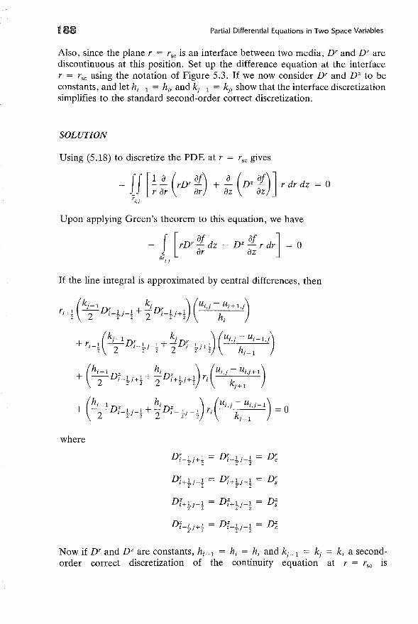
Also, since the plane r = rsc is an interface between two media, Dr and DZ arediscontinuous at this position. Set up the difference equation at the interfacer = rsc using the notation of Figure 5.3. If we now consider Dr and DZ to beconstants, and let hi- 1 = hi' and k j - 1 = k j , show that the interface discretizationsimplifies to the standard second-order correct discretization.

SOLUTION

Using (5.18) to discretize the PDE at r = rsc gives

-II [! i (rDr at) + ~ (Dz at)] r dr dz 0_ r ar ar az azr ..

'.}

Upon applying Green's theorem to this equation, we have

I [ at at]- rDr - dz - DZ - r dr = 0_ ar azar. .'.}

If the line integral is approximated by central differences, then

(h 1 h ) (u ..-U·· 1)+ ~Dz + -.!.Dz l,j I,j- - 0

. 1· 1 . 1· 1 r· -2 l-_,j-_ 2 l+-,j-_ 1 k

2 2 2 2 j-1

where

Di-l,j+l = Di-l,j-l = D~2 2 2 2

Df-£,j+£ = Df-l,j-l = D~2 2 2 2

Now if Dr and DZ are constants, hi- 1 hi = h, and k j - 1 = k j = k, a secondorder correct discretization of the continuity equation at r = rsc is


CORE SCREEN

(rj, Z j)

k j-I

(rj,zH)

r = rsc

FIGURE 5.3 Grid spacing at core-screen interface of annular bed reador.

(ri = ih, Zj = jk):

~: [(1 + ~) ui+1,j - 2ui,j + (1 - ~) U i - 1,j]

DZ+ k2 [Ui,j+1 - 2ui,j + Ui,j-1] = 0

Next, we will show that the interface discretization with the conditions statedabove simplifies to the previous equation. Since hi -1 = hi = hand kj -1 = kj = k,multiply the interface discretization equation by l/(hkri) to give

DZ+ k2 [Ui,j+1 - 2ui,j + ui,j-d 0

Notice that

ri+~ (i+ !)h 11 +-

r i ih 2i

ri+1 + ri-1 (i + !)h + (i - ~)h2 2 2r i ih

ri-1 (i - ~)h 12 1r i ih 2i


and that with these rearrangements, the previous discretization becomes thesecond-order correct discretion shown above.

Irregular Boundaries

Dirichlet Condition One method of treating the Dirichlet condition with irregular boundaries is to use unequal mesh spacings. For example, in figure SAa avertical mesh spacing from position B of f3h and a horizontal mesh spacing ofOI.h would incorporate aR into the discretization at the point B.

Another method of treating the boundary condition using a uniform meshinvolves selecting a new boundary. Referring to Figure SAa, given the curveaR, one might select the new boundary to pass through position B, that is,(xs, Ys)· Then, a zeroth-degree interpolation would be to take Us to bef(xs, Ys + f3h) or f(xs + OI.h, Ys) where w = f(x, y) on aR. The replacementof Us by f(xs, Ys + f3h) can be considered as interpolation at B by a polynomialof degree zero with value f(xs, Ys + f3h) at (xs, Ys + f3h). Hence the terminterpolation of degree zero. A more precise approximation is obtained by aninterpolation of degree one. A first-degree interpolation using positions Us andUc is:

Us - f(xs, Ys + f3h)f3h

or

Us = (f3 ~ l)UC + (f3 ~ l)f(xs, Ys + f3h)

Alternatively, we could have interpolated in the x-direction to give

Us = (01. : l)UA + (01. ~ l)f(xs + OI.h, Ys)

/3h

(5.25)

(5.26)

ilR

(0)

ilR

(b)

fiGURE 5.4 Irregular boundaries. (a) Uniform mesh with interpolation. (b) Nonuniform mesh with approximate boundary aRh'


Normal Derivative Conditions. Fortunately, in many practical applications normal derivative conditions occur only along straight lines, e.g., lines of symmetry,and often these lines are parallel to a coordinate axis. However, in the casewhere the normal derivative condition exists on an irregular boundary, it issuggested that the boundary aR be approximated by straight-line segments denoted aRh in Figure 5.4(b). In this situation the use of nonuniform grids isrequired. To implement the integration method at the boundary aRh' refer toFigure 5.5 during the following analysis. If b(xi, yJ :;f 0 in (5.14), then Ui,j isunknown. The approximation (5.22) can be used for vertical and horizontalportions of the line integral in Figure 5.5, but not on the portion denoted aRh'On aRh the normal to aRh makes an angle ewith the positive x-axis. Thus, aRhmust be parameterized by

x = Xi+1/2 - 'A sin e

and on aRh

Y = Yj-1/2 + 'A cos e

aWe' e- = Wx cos + wy sman

(5.27)

(5.28)

The portion of the line integral (Xi+1/2' Yj-1/2) to (Xi' y) in (5.20) can be writtenas

if if aw- (PWx cos e + PWy sin e) d'A = - P- d'A

o 0 an

FIGURE 5.5 Boundary point on aRh' Adapted from Richard S. Varga, Matrix IteratIveAnalysIs, © 1962, p. 184. Reprinted by permission of Prentice-Hali, Inc., EnglewoodCliffs, N. J.


or by using (5.14):

-L{PWx dy - PWy dx} = - LP [C(A) -b~A~A)W(A)] dA

= _ p . . [Ci,j - ai,jUi,j] .e (5.29)',j b· .

t,j

where

1.e = - Yh2 + k?

2 ' r 1 (path length of integration).

Notice that we have used the boundary condition together with the differentialequation to obtain a difference equation for the point (x;, y).

ELLIPTIC PDES-fINITE ELEMENTS

Background

Let us begin by illustrating finite element methods with the following ellipticPDE:

and

a2W a2 w

-2 + -2 = -f(x, y),ax ay for (x, y) in R (5.30)

W(x, y) = 0, for (x, y) on aR (5.31)

Let the bounded domain R with boundary aR be the unit square, that is, 0 :;:::; x :;:::; 1,o< Y :;:::; 1. Finite element methods find a piecewise polynomial (pp) approximation, u(x, y), to the solution of (5.30). The pp-approximation can be writtenas

m

u(x, y) = La/pix, y)j=l

(5.32)

where {<hex, y)lj = 1, ... ,m} are specified functions that satisfy the boundaryconditions and {ajlj = 1, ... , m} are as yet unknown constants.

In the collocation method the set {ajlj = 1, , m} is determined bysatisfying the PDE exactly at m points, {(Xi' Yi)li = 1, , m}, the collocationpoints in the region. The collocation problem for (5.30) using (5.32) as the ppapproximation is given by:

ACa = -f (5.33)

Elliptic PDES-Finite Elements

where

193

f = [I(x!> Yl), ... ,f(xm, Ym)]T

The solution of (5.33) then yields the vector Ol, which determines the collocationapproximation.

To formulate the Galerkin method, first multiply (5.30) by <Pi and integrateover the unit square:

II e:~ + ~:~) <Pi dx dy = - II f(x, Y)<Pi dx dyR R

i = i, ... ,m

Green's first identity for a function t is

II (at a<pi at a<pi) d d--+-- x Yax ax ay ay

R

II (aZt aZt) I at= - - + - <p. dx dy + - <p. deaxz ayz I an I

R M

(5.34)

(5.35)

where

~ = denotes differentiation in the direction of outward normalan

e = path of integration for the line integral

Since the functions <Pi satisfy the boundary condition, each <Pi is zero on aR.Therefore, applying Green's first identity to (5.34) gives

II (aw a<Pi + aw a<pi) dx dy = II f(x, y) <Pi dx dyax ax ay ay

R R

i = 1, ... ,m

For any two piecewise continuous functions 1] and <\1 denote

(1], <\1) = II 1]<\1 dx dyR

(5.36)

(5.37)

Equation (5.36) can then be written as

(V'w, V'<Pi) = (f, <Pi)'where

i = 1, ... ,m (5.38)

V' = gradient operator.


This formulation of (5.30) is called the weak form. The Galerkin method consistsin finding u(x) such that

i = 1, ... ,m (5.39)

or in matrix notation,

where

g = [gl> ... ,gmV

gi = (I, <Pi)

Next, we discuss each of these methods in further detail.

(5.40)

CollocationIn Chapter 3 we outlined the collocation procedure for BVPs and found thatone of the major considerations in implementing the method was the choice ofthe approximating space. This consideration is equally important when solvingPDEs (with the added complication of another spatial direction). The moststraightforward generalization of the basis functions from one to two spatialdimensions is obtained by considering tensor products of the basis functions forthe one-dimensional space !L?k(1T) (see Chapter 3). To describe these piecewisepolynomial functions let the region R be a rectangle with G1 ~ x ~ bv Gz ~ Y ~ b2J

where -00 < Gi ~ bi < 00 for i = 1,2. Using this region Birkhoff et al. [5] andlater Bramble and Hilbert [6,7] established and generalized interpolation resultsfor tensor products of piecewise Hermite polynomials in two space variables.To describe their results, let

(5.41)

h = max hi = max (X i + 1 - xJl~is.;;.Nx l:s:i~Nx

k = max k· = max (Yj+l - Yj)l,,;,j,,;,Ny J l,,;,j,,;,Ny

p = max {hJ k}

be the partitions in the x- and y-directions, and set 1T = 1Tl X 1T2' Denote byQ32(1T) the set of all real valued piecewise polynomial functions <Pi defined on

1T such that on each subrectangle [XiJ Xi+l] x [YjJ Yj+d of R defined by 1T, <Pi isa polynomial of degree at most 3 in each variable (x or y). Also, each <Pi'

Elliptic PDES-finite Elements 195

(a<p;)/(ax), and (a<p;)/(ay) must be piecewise continuous. A basis for !Z!2 is thetensor products of the Hermite cubic basis given in Chapter 3 and is

{V;(X)Vj(y), s;(x)Vj(Y)' v;(x)s/y), S;(X)Sj(Y)} [:1 [:1 (5.42)

where the v's and s's are listed in Table 3.2. If the basis is to satisfy the homogeneous Dirichlet conditions, then it can be written as:

i = 1,Nx + 1, j = 1, ... ,Ny + 1i=1, ,Nx +1, j=1,Ny +1i = 2, ,Nx , j = 2, ... ,Ny

(5.43)

Using this basis, Prenter and Russell [8] write the pp-approximation as:

Nx +1 N y +1 [ auu(x, y) = 2: 2: u(xb Yj)v;Vj + - (x;, Yj)S;Vj

;=1 j=1 ax (5.44)

au a2u ]+ - (x;, Y)V;Sj + -- (x;, Yj)S;Sjay ax ay

which involves 4(Nx + 1)(Ny + 1) unknown coefficients. On each subrectangle[x;, x;+d X [Yj' Yj+d there are four collocation points that are the combinationof the two Gaussian points in the x direction, and the two Gaussian points inthe Y direction, and are:

TL = (x; + ~ [1 - ~l Yj + 1[1- ~])

TT,j = (x; + ~ [1 + ~l Yj + 1[1-~])TL = (x; + ~ [1 - ~l Yj + 1[1+ ~])

Ttj = (x; + ~ [1 + ~l Yj + 1[1+ ~])

(5.45)

Collocating at these points gives 4Nx Ny equations. The remaining 4Nx + 4Ny + 4equations required to determine the unknown coefficients are supplied by theboundary conditions [37]. To obtain the boundary equations on the sides x = a1

and x = h1 differentiate the boundary conditions with respect to y. For example,if

au = y2 at x = a1 and x = h1ax

196

then


(5.46)

a2 u-- = 2y at x = a l and x = b Iax ay

Equation (5.46) applied at Ny - 1 boundary nodes (yjlj = 2, ... , Ny) gives:

auax (a v Yj) = yJ

a2uax ay (aI' y) = 2Yj

auax (b v Yj) = yJ

(5.47)

or 4Ny - 4 equations. A similar procedure at y = a2 and y = b2 is followed togive 4Nx - 4 equations. At each corner both of the above procedures are applied.For example, if

(5.48)

then

au ag- (av a2) = - (aI' a2)ay ay

Thus, the four corners supply the final 12 equations necessary to completelyspecify the unknown coefficients of (5.44).

EXAMPLE 3

Set up the colocation matrix problem for the PDE:

a2 w a2w- + - = <P °~ x ~ 1, °~ Y ~ 1ax2 ay2 '

with

w = 0, for x = 1

w= 0, for y = 1

aw0, for x = °-=

ax

aw0, for y = °-=

ay

Elliptic DPES-Finite Elements 197

where 1> is a constant. This PDE could represent the material balance of anisothermal square catalyst pellet with a zero-order reaction or fluid flow in arectangular duct under the influence of a pressure gradient. Let N x = Ny = 2.

SOLUTION

Using (5.44) as the pp-approximation requires the formulation of 36 equations.Let us begin by constructing the internal boundary node equations (refer toFigure 5.6a for node numberings):

aw (1, 2) = 0, a2w (1, 2)

ax ax ay

w(3,2)aw

0, ay (3,2) = 0

~; (2, 1) 0,a2 w-(2 1)ax ay ,

w(2, 3) = 0, aw (2, 3) 0ax

o

o

where w(i, j) w(x i, yJ At the corners

aw (1, 1) = aw (1, 1) = a2

w (1, 1) 0ax ay ax ay

aw a2 ww(l, 3) = - (1, 3) = - (1, 3) 0

ax ax ay

w(3,1) aw (3, 1) = a2

w (3, 1) 0ay ax ay

y y

,3)

(1,1)x

=0

1.0

~=oo y

w=O

V1V2 ,VI SZi'I S3 V2VZtV2SZ,V2S3

V2V2 ,V252/253 S2V2,5{>2,5253

S2V2'5252~2S, 5,v2,5?2'S3%w

VI VI' VI V2,VI~ V2V1,V2V2 ,V2~

v2v[ 1 V2V2,V2S; 52V,,52V2 ,5,A,

5 2V"S2V2'Sij, 53V,,53V2,~

1.0

ow =0ax

,2)

x(2,1) (3,1)

EI:COLLOCATION POINT

(i,j) : (x i' Yj )

(2,3)(3

EI EI EI EI

EI EI EI EI

(2,2) (3EI EI EI EI

EI EI EI EI

(1,2)

(1,3)

(0) (b)

fiGURE. 5.6 Grid for Example 3. (a) Collocation points. (b) Nonvanishing basisfunctions.

198

and


aw aww(3, 3) = - (3, 3) = - (3, 3) = 0

ax ay

This leaves 16 equations to be specified. The remaining 16 equations are thecollocation equations, four per subrectangle (see Figure 5.6a). If the aboveequations involving the boundary are incorporated in the pp-approximation,then the result is

U(x, y)

a=

where

U;,j = u(x;, Yj)

The pp-approximation is then used to collocate at the 16 collocation points.Since the basis is local, various terms of the above pp-approximation can bezero at a given collocation point. The nonvanishing terms of the pp-approximation are given in the appropriate subrectangle in Figure 5.6b. Collocating atthe 16 collocation points using the pp-approximation listed above gives thefollowing matrix problem:

where

1 = [1, ... , IV

[aUl Z aU13 auz 1

U U --'--'U --'UI,V I,Z' ay' ay' Z,V ax' z,z

auz,z auz,z aZuz,z aUZ,3 aZUZ,3ax' ay' ax ay' ay' ax ay

aU3,1 au3,z aZu3,z aZU3,3]Tax' ax' ax ay' ax ay

(for any function 1jJ)

and for the matrix A c,

-\C\C

A C =

V'IIIV1V 1V'IIIVlVZ V'I11V1SZ

V'II4VI Vl V'II4V I VZV'II4VlSZ

V'I11VZV 1V'I11SZV 1 V'IIIVZVZ V'Il1SZVZ V'I11VzSZ V'I11SzSZ

V'II4VZVl V'II4SZV l V'II4VZVZ V'II4S ZVZ V'II4VzSZ V'II4S zSZ

V'~ZIV2V2 V'~ZISZVZ V'~21VZSZ V'bszsz V'~ZIVZS3V'bSZS3

V'~Z4VZVZ V'~Z4SZVZ V'~Z4VZSZ V'~Z4S2SZ V'~Z4VZS3V'~Z4SZS3

V'11IS 3V 1

V'114S 3V :

V'~21S3VZ V'~ZIS3SZ V'bS3S3

V'~24S3V ZV'~Z4S3S2 V'~Z4S3S3


The solution of this matrix problem yields the vector a, which specifies the valuesof the function and its derivatives at the grid points.

Thus far we have discussed the construction of the collocation matrix problem using the tensor products of the Hermite cubic basis for a linear PDE. Ifone were to solve a nonlinear PDE using this basis, the procedure would be thesame as outlined above, but the ensuing matrix problem would be nonlinear.

In Chapter 3 we saw that the expected error in the pp-approximation whensolving BVPs for ODEs was dependent upon the choice of the approximatingspace, and for the Hermite cubic space, was O(h4). This analysis can be extendedto PDEs in two spatial dimensions with the result that [8]:

lu(x, y) - w(x, y)1 = O(p4)

Next, consider the tensor product basis for.!Z!'fe ('ITl) x .!Z!'fe ('ITz) where 'ITI andx y

'ITz are given in (5.41), kx is the order of the one-dimensional approximatingspace in the x-direction, and ky is the order of the one-dimensional approximatingspace in the y-direction. A basis for this space is given by the tensor productsof the B-splines as:

/

DIMX IDIMY

B;(x)B~(y) i~l j~l

where

Bf(x) = B-spline in the x-direction of order kx

B~(y) = B-spline in the y-direction or order ky

DIMX = dimension of .!Z!t

DIMY = dimension of .!Z! 'fey

The pp-approximation for this space is given by

DIMX DIMY

u(x, y) = 2: 2: (Xi,jBf(x)B~(y)i~ 1 j= 1

where (Xi,j are constants, with the result that

lu(x, y) - w(x, y)1 = O(p'!)

where

(5.49)

(5.50)

(5.51)

Galerkin

The literature on the use of Galerkin-type methods for the solution of ellipticPDEs is rather extensive and is continually expanding. The reason for this growthin use is related to the ease with which the method accommodates complicated


geometries. First, we will discuss the method for rectangles, and then treat theanalysis for irregular geometries.

Consider a region R that is a rectangle with a l ~ x ~ bl , a2 ~ Y ~ b2, with-00 < ai ~ bi < 00 for i = 1,2. A basis for the simplest approximating spaceis obtained from the tensor products of the one-dimensional basis of the space..0i(1T), i.e., the piecewise linears. If the mesh spacings in x and yare given by1TI and 1T2 of (5.41), then the tensor product basis functions wi,/x, y) are givenby

[x - Xi-I] [Y - Yj-ll Xi- l ~ x~ Xi' Yj-l ~ Y ~ Yjhi- l kj- l

[X - Xi-I] [Yj+l - Y1 Xi- l ~ X ~ Xi' Yj~Y ~Yj+lhi- l kj

Wi,j (5.52)

[Xi+l - X] [Y-Yj-l} Xi~X~Xi+h Yj-l ~ Y ~ Yjh, k j - l

[Xi+lhi- X] [Yj+lkj- Y1 Xi ~ X ~ Xi+h Yj~Y~Yj+1

with a pp-approximation of

Nx+l Ny+lu(x, y) = L L U(Xi' Yj)Wi,j

i= I j= I(5.53)

Therefore, there are (Nx + l)(Ny + 1) unknown constants u(xi , y), eachassociated with a given basis function Wi,j' Figure 5.7 illustrates the basis functionWi,j' from now on called a bilinear basis function.

EXAMPLE 4

Solve (5.30) with f(x, y) 1 using the bilinear basis with Nx = Ny = 2.

fiGURE 5.7 Bilinear basis function.


SOLUTION

The PDE is

0<;; x <;; 1, 0 <;; Y <;; 1

with

w(x, y)

The weak form of the PDE is

o on the boundary

II (aw a<Pi aw a<pi) II- -- + - -- dx dy = <Pi dx dyax ax ay ay

R R

where each <Pi satisfies the boundary conditions. Using (5.53) as the pp-approximation gives

3 3

u(x, y) = 2: 2: u(xi, Yj)Wi,ji~ 1 j~ 1

Let hi = k j = h = 0.5 as shown in Figure 5.8, and number each of the subrectangles, which from now on will be called elements. Since each Wi,j mustsatisfy the boundary conditions,

leaving the pp-approximation to be

u(x, y) = u(xz, yz)wz,z = UzWz

y

x1.0

U 1,3 U 2 ,3 U 3,3

® CDU 1,2 U2,2 U 3,2

® @

U',I U 2tl U 3,Ioo

1.0

fiGURE 5.8 Grid for Example 4. CD = element I.


Therefore, upon substituting u(x, y) for w(x, y), the weak form of the PDEbecomes

II ( awz awz awz awz) IIUz - - + Uz - - dx dy = Wz dx dyax ax ay ay

R R

or

where

II (awz awz + awz awz) dx dAzz = ax ax ay ay y

R

gz = II Wz dx dyR

This equation can be solved on a single element ei as

ei = 1, ... ,4

and then summed over all the elements to give

4 4

Azzuz = L A~2UZ = L g~; = gzei=l ej=l

In element 1:

Uzu(x, y) = hZ (1 - x)(l - y),

and

0.5 ~ x ~ 1, 0.5 ~ Y ~ 1

1W z = hZ (1 - x)(l - y)

Thus

Aiz = h14 e e [(1 - yf + (1 - x)Z] dx dy = ~)0.5 )0.5 3

and

gi = 1z f e (1 - x)(l - y) dx dy = hZ

h 0.5 )0.5 4

For element 2:

(h = 0.5)

Uzu(x, y) = hZ (1 - y)x, o~ x ~ 0.5, 0.5 ~ Y ~ 1.0

204

and

giving

and


1W z = hZ x(l - Y)

The results for each element are

Element Aei22

12'3

2 23

3 :<3

4 23

Thus, the solution is given by the sum of these results and is

Uz = i hZ = 0.09375

In the previous example we saw how the weak form of the PDE could besolved element by element. When using the bilinear basis the expected error inthe pp-approximation is

Iu(x, Y) - w(x, Y)I = O(pZ) (5.54)

(5.55)

where p is given in (5.41). As with ODEs, to increase the order of accuracy,the order of the tensor product basis functions must be increased, for example,the tensor product basis using Hermite cubics given an error of 0(p4). To illustratethe formulation of the Galerkin method using higher-order basis functions, letthe pp-approximation be given by (5.50) and reconsider (5.30) as the ellipticPDE. Equation (5.39) becomes

(V ~~x ~~y (Xi,jB~(x)B;(y), VB;';,(X)B~(Y)) = 0B;';,(X)B~(Y))

m = 1, ... , DIMX, n = 1, ... , DIMY

In matrix notation (5.55) is

Aa = g (5.56)

Elliptic DPES-Finite Elements

where

_ [- - ]Tg - gl>"" gz

gj = [(f, B:(x)B{(y)), ... , (f, B:(x)Bt>IMy(y))]T

Ap,q = (VB:(x)Br(y), VB~,(x)B~(y))

p = DIMY (m - 1) + n (1 ~ P ~ DIMX x DIMY)

q = DIMY (i - 1) + j (1 ~ q ~ DIMX x DIMY)

Equation (5.56) can be solved element by element as

No. of elements No. of elements

L Aiq<Xq = L giei=l ei=l

205

(5.57)

The solution of (5.56) or (5.57) gives the vector a, which specifies the ppapproximation u(x, y) with an error given by (5.51).

Another way of formulating the Galerkin solution to elliptic problems isthat first proposed by Courant [9]. consider a general plane polygonal region Rwith boundary aR. When the region R is not a rectangular parallelepiped, arectangular grid does not approximate R and especially aR as well as a triangulargrid, i.e., covering the region R with a finite number of arbitrary triangles. Thispoint is illustrated in Figure 5.9. Therefore, if the Galerkin method can beformulated with triangular elements, irregular regions can be handled throughthe use of triangulation. Courant developed the method for Dirichlet-type boundaryconditions and used the space of continuous functions that are linear polynomialson each triangle. To illustrate this method consider (5.30) with the pp-approximation (5.32). If there are TN vertices not on aR in the triangulation, then(5.32) becomes

TN

u(x, y) = L <Xs<Ps(x, y)s~l

(5.58)

Given a specific vertex s = e, <Xe = u(xf, Ye) with an associated basis function<l>e(x, y). Figure 5.lOa shows the vertex (xeo Ye) and the triangular elements thatcontain it, while Figure 5.10b illustrates the associated basis function. The weakform of (5.30) is

II (au a<l>s + au a<l>s) dx dy = II f(x, Y)<l>s dx dyax ax ay ay

R R

s = 1, ... , TN (5.59)

206

(0)


(b)

fiGURE 5.9 Grids on a polygonal region. (a) Rectangular grid. (b) Triangular grid.

or in matrix notation

Aa = g

where

A sq = JJ [a<ps a<pq + a<ps a<pq] dx dyax ax ay ay

R

g = [JJf(x, Y)<Pl dx dy, ... , JJf(x, y)<PTN dx dY] T

R R

(5.60)

(0) (b)

fiGURE 5.10 Linear basis function for triangular elements. (a) Vertex (xe, Ye)' (b)Basis function <Pe.


Equation (5.60) can be solved element by element (triangle by triangle) andsummed to give

2: A;~aq = 2: g;iei ej

s = 1, ... , TN, q = 1, ... , TN (5.61)

Since the PDE can be solved element by element, we need only discuss theformulation of the basis functions on a single triangle. To illustrate this formulation, first consider a general triangle with vertices (Xi' Yi), i = 1, 2, 3. Alinear interpolation Pl(x, y) of a function C(x, y) over the triangle is given by[10]:

where

3

Pl(x, y) = 2: a;(x, Y)C(Xb y;)i=l

al(x, y) = l/J(-r23 + 'll23X - ~23Y)

a2(x, y) = l/J(-r3l + 'll3lX - ~3lY)

a3(x, y) = l/J(T12 + 'll12X - ~12Y)

l/J = (twice the area of the triangle)-l

(5.62)

To construct the basis function <Pe associated with the vertex (xe, Ye) on a singletriangle set (xe, Ye) = (Xl, Yl) in (5.62). Also, since <Pe(xe> Ye) = 1 and <Pe iszero at all other vertices set C(xl, Yl) = 1, C(x2, Y2) = 0 and C(X3' Y3) = 0 in(5.62). With these substitutions, <Pe = PI(X, y) = al(x, y). We illustrate thisprocedure in the following example.

EXAMPLE 5

Solve the problem given in Example 3 with the triangulation shown in Figure5.11.

SOLUTION

From the boundary conditions


y

1.0U 1,3 U 2,3 U 3,3

® ®

CD ®U 1,2 U 2,2 U 3,2

@) ®

® CDU 2,I U 3,I

X

0 1.0

fiGURE 5.11 Triangulation for Example 5. CD = element J

Therefore, the only nonzero vertex is uz,z, which is common to elements 2, 3,4, 5, 6, and 7, and the pp-approximation is given by

u(x, y) = uz,z<Pz(x, y) = uz<Pz

Equation (5.61) becomes7 7

~ A~2Uz = ~ g~iei=2 ei=2

where

A ei = JJ (a<pz a<pz + a<pz a<pz) dx dzz ax ax ay ay y

Triangleei

Triangleei

The basis function <p~i can be constructed using (5.62) with (Xl> Yl) = (0.5,0.5)giving

Thus,

e,

Elliptic DPES-Finite Elements

and

ei

For element 2 we have the vertices

(Xl' Yl) = (0.5, 0.5)

(X2' Y2) = (1, 0.5)

(x3 , Y3) = (0.5, 0)

and

1tV = 0.25

1"23 = (1)(0) - (0.5)(0.5) = - 0.25

~23 = 1 - 0.5 = 0.5

1123 = 0.5

A~2 = II (0.25)-2[(0.5)2 + (0.5)2] dx dy = 1

2 - II 1 ] _ 0.25g2 - (0.25) [-0.25 + 0.5x - 0.5y dx dy - -6-

Likewise, the results for other elements are

Element Aei g;i22

0.252 1.0 -

6

0.50.25

3 -6

0.50.25

4 -6

0.255 0.5 -

6

0.50.25

6 -6

0.257 1.0 -

6-

Total 4.0 0.25

which gives

U2 = 0.0625

209

210

C3


c,

(a)

C2

( b)

fiGURE 5. t 2. Node positions for triangular elements. (a) Linear basis. (b) Quadraticbasis: C, = C(x" y,).

The expected error in the pp-approximation using triangular elements withlinear basis functions is O(h2

) [11], where h denotes the length of the largest sideof any triangle. As with rectangular elements, to obtain higher-order accuracy,higher-order basis functions must be used. If quadratic functions are used tointerpolate a function, C(x, Y), over a triangular element, then the interpolationis given by [10]:

where

6

L bi(x, y)C(x, y)i= 1

(5.63)

j = 1, 2, 3b/x, y) = aj(x, y)[2aj(x, y) - 1],

b4(x, y) = 4a1(x, y)a2(x, y)

bs(x, y) = 4a 1(x, y)a3(x, y)

b6(x, y) = 4aix, y)a3(x, y)

and the ai(x, y)'s are given in (5.62). Notice that the linear interpolation (5.62)requires three values of C(x, y) while the quadratic interpolation (5.63) requiressix. The positions of these values for the appropriate interpolations are shownin Figure 5.12. Interpolations of higher order have also been derived, and goodpresentations of these bases are given in [10] and [12].

Now, consider the problem of constructing a set of basis functions for anirregular region with a curved boundary. The simplest way to approximate thecurved boundary is to construct the triangulation such that the boundary isapproximated by the straight-line segements of the triangles adjacent to theboundary. This approximation is illustrated in Figure 5.9b. An alternative procedure is to allow the triangles adjacent to the boundary to have a curved sidethat is part of the boundary. A transformation of the coordinate system canthen restore the elements to the standard triangular shape, and the PDE solvedas previously outlined. If the same order polynomial is chosen for the coordinatechange as for the basis functions, then this method of incorporating the curved

Parabolic PDES in Two Space Variables 211

boundary is called the isoparametric method [10-12]. To outline the procedure,consider a triangle with one curved edge that arises at a boundary as shown inFigure 5.13a. The simplest polynomial able to describe the curved side of thetriangular element is a quadratic. Therefore, specify the basis functions for thetriangle in the Al-A2 plane to be quadratics. These basis functions are completelyspecified by their values at the six nodes shown in Figure 5.13b. Thus theisoparametric method maps the six nodes in the x-y plane onto the ACA2 plane.The PDE is solved in this coordinate system, giving U(Al> A2), which can betransformed to u(x, y).

PARABOLIC PDES IN TWO SPACE VARIABLES

In Chapter 4 we treated finite difference and finite element methods for solvingparabolic PDEs that involved one space variable and time. Next, we extend thediscussion to include two spatial dimensions.

Method of Lines

Consider the parabolic PDE

aw = D [a 2 w + a2 w]at ax2 ay2

oR

o~ t, o~ x ~ 1, (5.64)

( 0)

(O,I)

-----...~II--....-----... },.,(0,0) (1,0)

( b)

fiGURE. 5.13 C.oordinate transformation. (a) xy-plane. (b) AtAz-plane.


(5.65)

with D constant. Discretize the spatial derivatives in (5.64) using finite dif-ferences to obtain the following system of ordinary differential equations:

au·· D Da~'J = (LiX)JUi+1,j - 2ui,j + Ui-1J + (Liy)JUi,j+l - 2ui,j + Ui,j-l]

where

Ui,j = w(xiJ y)

Xi = i Lix

Yj = j Liy

Equation (5.65) is the two-dimensional analog of (4.6) and can be solved in asimilar manner. To complete the formulation requires knowledge of the subsidiary conditions. The parabolic PDE (5.64) requires boundary conditions at X = 0,x = 1, y = 0, and y = 1, and an initial condition at t = 0. As with the MOLin one spatial dimension, the two-dimensional problem incorporates the boundary conditions into the spatial discretizations while the initial condition is usedto start the IVP.

Alternatively, (5.64) could be discretized using Galerkin's method or bycollocation. For example, if (5.32) is used as the pp-approximation, then thecollocation MOL discretization is

(5.66)

i = 1, ... ,m

where (Xi> y;) designates the position of the ith collocation point. Since the MOLwas discussed in detail in Chapter 4 and since the multidimensional analogs arestraightforward extensions of the one-dimensional cases, no rigorous presentation of this technique will be given.

Alternating Direction Implicit Methods

Discretize (5.65) in time using Euler's method to give

ut,j = [~~~] [U?+l,j + U?-l,j] + [~~;] [Ui,j+l + Ui,j-l]

[2D Lit 2D Lit]

+ ui,j 1 - (LiX)2 - (Liy)Z

where

(5.67)

Parabolic PDES in Two Space Variables

For stability

[ 1 1] 1D ilt (ilX)2 + (ily)2 < 2"

If ilx = ily, then (5.68) becomes

D ilt 1--~

(ilX)2 4

213

(5.68)

(5.69)

(5.70)

which says that the restriction on the time step-size is half as large as the onedimensional analog. Thus the stable time step-size decreases with increasingdimensionality. Because of the poor stability properties common to explicitdifference methods, they are rarely used to solve multidimensional problems.Inplicit methods with their superior stability properties could be used instead ofexplicit formulas, but the resulting matrix problems are not easily solved. Another approach to the solution of multidimensional problems is to use alternatingdirection implicit (ADI) methods, which are two-step methods involving thesolution of tridiagonal sets of equations (using finite difference discretizations)along lines parallel to the x-y axes at the first-second steps, respectively.

Consider (5.64) with D = 1 where the region to be examined in (x, y, t)space is covered by a rectilinear grid with sides parallel to the axes, andh = ilx = ily. The grid points (Xi' yj' tn ) given by x = ih, Y = jh, and t = n ilt,and ui,j is the function satisfying the finite difference equation at the grid points.Define

iltT = h2

Essentially, the principle is to employ two difference equations that are used inturn over successive time-steps of ilt/2. The first equation is implicit in the xdirection, while the second is implicit in the y-direction. Thus, if Ui,j is an intermediate value at the end of the first time-step, then

or

Ui,j un. T [ 2- + O~Ui,J= 2" °XUi,jl,J

Un+ 1 U· . T [ 2- + 02Un+l]= 2" °xUi,jl,J l,J Y l,J

[1 - ! Tonti = [1 + ! TO~]Un

[1 - !To~]Un+l = [1 + !Tonti

(5.71)

(5.72)

214

where


for all i and j

These formulas were first introduced by Peaceman and Rachford [13], andproduce an approximate solution which has an associated error of O(Lit2 + h2 ).

A higher-accuracy split formula is due to Fairweather and Mitchell [14] and is

[1 - H,. - ~) 8;]ii = [1 + H,. + ~) 8~]un

[1 - ~ (,. - ~) 8~]un+l = [1 + ~ (,. + ~) 8~]ii (5.73)

with an error of O(Llt2 + h4). Both of these methods are unconditionally stable.A general discussion of ADI methods is given by Douglas and Gunn [15].

The intermediate value ii introduced in each ADI method is not necessarilyan approximation to the solution at any time level. As a result, the boundaryvalues at the intermediate level must be chosen with care. If

W(x, y, t) = g(x, y, t) (5.74)

when (x, y, t) is on the bounadry of the region for which (5.64) is specified,then for (5.72)

and for (5.73)

Ui,j = ,. ~ ~ [1 - HT - n8~]gZ:1 + ,. ; ~ [1 + HT + ~) 8~]gi,j

(5.75)

(5.76)

If g is not dependent on time, then

Ui,j = gi,j (for 5.72) (5.77)

Ui,j = (1 + ~ 8~)gi,j (for 5.73) (5.78)

A more detailed investigation of intermediate boundary values in ADI methodsis given in Fairweather and Mitchell [16].

ADI methods have also been developed for finite element methods. Douglas and Dupont [17] formulated ADI methods for parabolic problems usingGalerkin methods, as did Dendy and Fairweather [18]. The discussion of thesemethods is beyond the scope of this text, and the interested reader is referredto Chapter 6 of [11].

MATHEMATICAL SOFTWARE

As with software for the solution of parabolic PDEs in one space variable andtime, the software for solving multidimensional parabolic PDEs uses the methodof lines. Thus a computer algorithm for multidimensional parabolic PDEs based

Mathematical Software 215

(5.79)

upon the MOL must include a spatial discretization routine and a time integrator.The principal obstacle in the development of multidimensional PDE softwareis the solution of large, sparse matrices. This same problem exists for the development of elliptic PDE software.

ParabolicsThe method of lines is used exclusively in these codes. Table 5.1 lists the parabolicPDE software and outlines the type of spatial discretization and time integrationfor each code. None of the major libraries-NAG, Harwell, and IMSL-containmultidimensional parabolic PDE software, although 2DEPEP is an IMSL product distributed separately from their main library. As with one-dimensional PDEsoftware, the overwhelming choice of the time integrator for multidimensionalparabolic PDE software is the Gear algorithm. Next, we illustrate the use oftwo codes.

Consider the problem of Newtonian fluid flow in a rectangular duct. Initially, the fluid is at rest, and at time equal to zero, a pressure gradient is imposedupon the fluid that causes it to flow. The momentum balance, assuming a constantdensity and viscosity, is

av Po - PL [a 2v a2v]p-= +/-L-+-at L ax2 ay2

TABLE 5.1 Parabolic PDE Codes

Spatial Discretiza- SpatialCode tion Time Integrator Dimension Region Reference

DSS/2 Finite difference Options including 2or3 Rectangular [19]Runge-Kutta andGEARB [24]

PDETWO Finite difference GEARB [24] 2 Rectangular [20]FORSIM VI Finite difference Options including 2or3 Rectangular [21]

Runge-Kutta andGEAR [25]

DISPL Finite element; Gal- Modified version of 2 Rectangular [22]erkin with tensor GEAR [25]products of B-spli-nes for the basisfunction

2DEPEP Finite element; Gal- Crank-Nicolson or an 2 Irregular [23]erkin with quad- implicit methodratic basis functionson triangular ele-ments; curvedboundaries incor-porated by isopara-metric method

216

where


p = fluid density

Po - PL .L = pressure gradIent

J1. = fluid viscosity

V = axial fluid velocity

The situation is pictured in Figure 5.14. Let

xX=B

y=Lw

V

J1.!T=-

pB2 (5.80)

Substitution of (5.80) into (5.79) gives

aT] a 2T]-=2+-+aT a2x

The subsidiary conditions for (5.81) are

(B)2 a2T]

w a2y(5.81)

T] = 0 at T = 0 (fluid initially at rest)

T] = 0 at y=O (no slip at the wall)

T] = 0 at X=1 (no slip at the wall)

aT] = 0 at X = 0 (symmetry)ax

aT] = 0 at Y = 1 (symmetry)aY

Equation (5.81) was solved using DISPL (finite element discretization) andPDETWO (finite difference discretization). First let us discuss the numericalresults form these codes. Table 5.2 shows the affect of the mesh spacing(klY = klX = h) when solving (5.81) with PDETWO. Since the spatial discretization is accomplished using finite differences, the error associated with this

Mathematical Software 217

y

L

~~2W---<?"""'-~LUID OUT

ff------t"xFLUIDIN

fiGURE 5.14 flow In a rectangular duct.

discretization is 0(h2 ). As h is decreased, the values of 'Y] shown in Table 5.2increase slightly. For mesh spacings less than 0.05, the same results were obtainedas those shown for h = 0.05. Notice that the tolerance on the time integrationis 10-7 , so the error is dominated by the spatial discretization. When solving(5.81) with DISPL (cubic basis functions), a mesh spacing of h = 0.25 producedthe same solution as that shown in Table 5.2 (h = 0.05). This is an expectedresult since the finite element discretization is 0(h4 ).

Figure 5.15 shows the results of (5.81) for various X, Y, and 'I". In Figure5.15a the affect at the Y-position upon the velocity profile in the X-direction isillustrated. Since Y = 0 is a wall where no slip occurs, the magnitude of thevelocity at a given X-position will increase as one moves away from the wall.Figure 5.15b shows the transient behavior of the velocity profile at Y = 1.0. Asone would expect, the velocity increases for 0 ~ X < 1 as ,. increases. This trendwould continue until steady state is reached. An interesting question can nowbe asked. That is, how large must the magnitude of W be in comparison to themagnitude of B to consider the duct as two infinite parallel plates. If the ductin Figure 5.14 represents two infinite parallel plates at X = ±1, then the

BTABLE 5.2 Results of (5.81) Using PDETWO: ,. = 0.5, W= 1, Y = 1, TOL = 10- 7

'Y]

X h = 0.2 h = 0.1 h = 0.05

0.0 0.5284 0.5323 0.53330.2 0.5112 0.5149 0.51590.4 0.4575 0.4608 0.46170.6 0.3614 0.3640 0.36460.8 0.2132 0.2146 0.21501.0 0 0 0


0.6 ,.--,----,---,.--,----,

1. (b) Y = 1.0, BIW = 1.

LO08

!

0.2 0.4 0.6

X

(b)

(l) 1.00(1) 0.75(3) 0.50(4) 0.15

0.2

0.1

0.5

0.4

TJ 0.3

1.00.6 0.80.4

X

(a)

Results of (5.81).(et) 'T = 0.15, BIW =

Y

(1) 0.15(1) 0.5(3) 1.0

0.2

0.1

0.0 '--_--'--_--'-_---'L.--_--'--_~

o

0.5

0.4

0.3

TJ(2)

0.2

fiGURE 5.15

momentum balance becomes

(5.82)

with

T) = 0 at 'T = 0

T) = 0 at X= 1

aT) = 0 at X = 0axEquation (5.82) possesses an analytic solution that can be used in answering theposed question. Figure 5.16 shows the affect of the ratio B/W on the velocityprofile at various 'T. Notice that at low 'T, a B/W ratio of ~ approximates theanalytical solution of (5.82). At larger 'T this behavior is not observed. To matchthe analytical solution (five significant figures) at all 'T, it was found that thevalue of B/W must be i or less.

Mathematical Software

1.0 ,---,-----,---,----,----,

119

1.0 ,---,-----,---,---,-----,

r =0.5

Y = 1.00.8

0.6

0.4

0.2

0.8

0.6

0.4

02

(3)r= 1.0

Y =1.0

0.0 '--_...L-_--'--__"---_-"-_--'" 0.0 '---_...L-_-----'-__'--_-'-_-'"o 0.2 0.4 0.6 0.8 1.0 0 0.2 0.4 0.6 0.8 1.0

x

FIGURE. 5.16 further results of (5.81).

BIW(1) 1(2) 1/z(3) 1/4 and analytical solution of (5.82)

x

Ellipties

Table 5.3 lists the elliptic PDE software and outlines several features of eachcode. Notice that the NAG library does contain elliptic PDE software, but thisroutine is not very robust. Besides the software shown in Table 5.3, DISPL and2DEPEP contain options to solve elliptic PDEs. Next we consider a practicalproblem involving elliptic PDEs and illustrate the solution and physical implications through the use of DISPL.

The most common geometry of catalyst pellets is the finite cylinder withlength to diameter, LID, ratios from about 0.5 to 4, since they are produced byeither pelleting or by extrusion. The governing transport equations for a finitecylindrical catalyst pellet in which a first-order chemical reaction is occurringare [34]:

where

(Mass)

(Energy)

( )2 []

(Pf 1 af D a2f 'Y- + - - + - - = <p 2f exp - (t - 1)ar 2 r ar L az2 t

( )2 []

a2t 1 at D a2t 2 'Y- + - - - - = -!3<P f exp - (t - 1)ar 2 r ar L az2 t

(5.83)

r = dimensionless radial coordinate, 0 ~ r ~ 1z = dimensionless axial coordinate, 0 ~ z ~ 1

220

f=t =

'Y<P13


dimensionless concentrationdimensionless temperatureArrhenius number (dimensionless)Thiele modulus (dimensionless)Prater number (dimensionless)

with the boundary conditions

af at= 0 at r = 0ar ar

af at0 0- at zaz az

(symmetry)

(symmetry)

f = t = 1 at z = 1 and r 1 (concentration andtemperature specified atthe surface of the pellet)

Using the Prater relationship [35], which is

t = 1 + (1 - f)l3

TABLE 5.3 Elliptic POE Codes

NonlinearEquations Reference

No

No [26]No [27]No [28]No [29]No [30]

No [31]

Code

NAG(D03 chapter)

FISPACKEPDE1ITPACK/REGIONFFf9HLMHLZ/HEL-

MIT/HELSIXIHELSYM

PLTMG

ELIPTI

ELLPACK

Discretization

Finite difference(Laplace's equation

in two dimensions)Finite differenceFinite differenceFinite differenceFinite differenceFinite difference

Finite element; Galerkin with linearbasis functions ontriangular elements

ADI with finite differences; integrateto steady state

Finite difference; finite element (collocation and Galerkin)

Region

Rectangular

RectangularIrregularIrregularIrregularIrregular

Irregular

Irregular

Rectangular

Yes

Yes

[32]

[33]

Mathematical Software

TABlE. 5.4 Results of (5.84) Using DlSPLD

Jl = 0.25,13 = 0.1, 'Y = 30, - =L

221

$=1

r h = 0.5 h = 0.25

0 0.728 0.7280.25 0.745 0.7450.50 0.797 0.7970.75 0.882 0.8821.0 1.000 1.000

h = 0.50.724( -3)0.384( -1)0.1090.4141.000

$ = 2

h = 0.25

0.240( -1)0.377( -1)0.1150.4041.000

h = 0.125

0.227( -1)0.365( -1)0.1150.4041.000

reduces the system (5.83) to the single elliptic PDE:

( )2 [ ]

a2f 1 af D a2f 2 'Y13(1 - f)ar 2 + -;. ar + L az2 = <P J exp 1 + 13(1 - f)

af = 0 at r = 0ar

(5.84)

af = 0 at z = 0az

f = 1 at r = 1 and z = 1

DISPL (using cubic basis functions) produced the results given in Tables5.4 and 5.5 and Figure 5.17. In Table 5.4 the affect of the mesh spacing(h = fJ.r = fJ.z) is shown. With $ = 1 a coarse mesh spacing (h = 0.5) issufficient to give three-significant-figure accuracy. At larger values of <p a finermesh is required for a similar accuracy. As <p increases, the gradient in f becomes larger, especially near the surface of the pellet. This behavior is shownin Figure 5.17. Because of this gradient, a finer mesh is required to obtain anaccurate solution over the entire region. Alternatively, one could refine themesh in the region of the steep gradient. Finally, in Table 5.5 the isothermalresults (13 = 0) are compared with those published elsewhere [34]. As shown,DISPL produced accurate results with h = 0.25.

TABlE. 5.5 Further Results of (5.84) Using DISPLL

13 = 0.0, 'Y = 30, $ = 3, D = 1

(r, z)

(0.394, 0.285)(0.394, 0.765)(0.803, 0.285)(0.803, 0.765)

DISPL,h = 0.25

0.3370.5850.6480.756

FromReference [34]

0.3370.5850.6480.759

222 Partial Differential E.quations in Two Space Variables

1.000750.50

1.10 F=:::::::J:::::-----,---,---i

1.08

1.06

1.02

1.04

1.00 ,------,-----,---,,-----.1

0.20

0.40

060

080

0.00 ~=::::J=-_--.JL___L__--.J 1.00 ~--~--~-~--~0.00 0.25 0.50 0.75 1.00 0.00 0.25

fiGURE. 5.17 Results of (5.84): p = 0.1, 'Y = 30, <I> = 2, DIL = 1.

!(1) 0.75(2) 0.50(3) 0.00

PROBLEMS

1. Show that the finite difference discretization of

a2 w a2 w(x + 1) - + (y2 + 1) - - w = 1ax 2 ay 2

o :%; x:%; 1, 0 :%; Y :%; 1, Lix = Liy = ~

with

w(O, y) = Y

w(l, y) = y2

w(x,O) = 0

w(x, 1) = 1

is given by [36]:

Problems 223

2.* Consider a rectangular plate with an initial temperature distribution of

w(x, y, 0) = T - To = 0, °~ x ~ 2, °~ y ~ 1

°~ r ~ 1, °~ z ~ 1

3.*

If the edges x = 2, y = 0, and y = 1 are held at T = To and on the edgex = °we impose the following temperature distribution:

() {2tY for °~ Y ~ ~

w 0, Y, t = T - To = 2t(1' _ y), f 1 1or 2: ~ Y ~

solve the heat conduction equation

aw a2w a2w-=-+-at ax2 ay 2

for the temperature distribution in the plate. The analytical solution tothis problem is [22]:

w = ± i i ~ \ (e-O"! + at - 1) sin (WIT) sin (m'Trx) sin (n'TrY)'Trm~ln=ln a 2 2

where

a = 'Tr2 (:2 + n2 )

Calculate the error in the numerical solution at the mesh points.

An axially dispersed isothermal chemical reactor can be described by thefollowing material balance equation:

at = _1 [a2t + ! at] + _1_ a2t + Daz Per ar2 r ar Pea az2 at,

with

1 - t = _1_ at at zPea az

0, at = ° at r = °and r = 1ar

ataz ° a. z = 1

wheret = dimensionless concentration

r = dimensionless radial coordinate

z = dimensionless axial coordinate

Per = radial Peclet number

Pea = axial Peclet number

D a = Damkohler number (first-order reaction rate)


The boundary conditions in the axial direction arise from continuity offlux as discussed in Chapter 1 of [34]. Let Da = 0.5 and Per = 10. Solvethe material balance equation using various values of Pea' Compare yourresults to plug flow (Pea -? (0) and discuss the effects of axial dispersion.

4.* Solve Eq. (5.84) with D/L = 1, <p = 1, "y = 30, and let -0.2 ~ 13 ~ 0.2.Comment on the affect of varying 13 [13 < 0 (endothermic), 13 > 0 (exothermic)].

5.* Consider transient flow in a rectangular duct, which can be described by:

a'Y] = a + a2

'Y] + (B) 2 a2

'Y]aT aX2 w ay2

using the same notation as with Eq. (5.81) where a: is a constant. Solvethe above equation with

-(l( Comment

(a) 2(b) 4(c) 1

Eq. (5.81)Twice the pressure gradient as Eq. (5.81)Half the pressure gradient as Eq. (5.81)

How does the pressure gradient affect the time required to reach steadystate?

REFE.RENCE.S

1. Bank, R. E., and D. J. Rose, "Parameter Selection for Newton-LikeMethods Applicable to Nonlinear Partial Differential Equations: SIAM J.Numer. Anal., 17, 806 (1980).

2. Denison, K. S., C. E. Hamrin, and J. C. Diaz, "The Use of PreconditionedConjugate Gradient and Newton-Like Methods for a Two-Dimensional,Nonlinear, Steady-State, Diffusion, Reaction Problem," Comput. Chern.Eng., 6, 189 (1982).

3. Denison, K. S., private communication (1982).

4. Varga, R. S., Matrix Iterative Analysis, Prentice-Hall, Englewood Cliffs,N.J. (1962).

5. Birkhoff, G., M. H. Schultz, and R. S. Varga, "Piecewise Hermite Interpolation in One and Two Variables with Applications to Partial Differential Equations," Numer. Math., 11, 232 (1968).

6. Bramble, J. H., and S. R. Hilbert, "Bounds for a Class of Linear Functionals with Applications to Hermite Interpolation," Numer. Math., 16,362 (1971).

References 225

7. Hilbert, S. R., "A Mollifier Useful for Approximations in Sobolev Spacesand Some Applications to Approximating Solutions of Differential Equations," Math. Comput., 27, 81 (1973).

8. Prenter, P. M., and R. D. Russell, "Orthogonal Collocation for EllipticPartial Differential Equations," SIAM J. Numer. Anal., 13, 923 (1976).

9. Courant, R., "Variational Methods for the Solution of Problems of Equilibrium and Vibrations," Bull. Am. Math. Soc., 49, 1 (1943).

10. Mitchell, A. R., and R. Wait, The Finite Element Method in Partial Differential Equations, Wiley, London (1977).

11. Fairweather, G., Finite Element Galerkin Methods for Differential Equations, Marcel Dekker, New York (1978).

12. Strang, G., and G. J. Fix, An Analysis of the Finite Element Method,Prentice-Hall, Englewood Cliffs, N.J. (1973).

13. Peaceman, D. W., and H. H. Rachford, "The Numerical Solution ofParabolic and Elliptic Differential Equations," J. Soc. Ind. Appl. Math.,3, 28 (1955).

14. Mitchell, A. R., and G. Fairweather, "Improved Forms of the AlternatingDirection Methods of Douglas, Peaceman and Rachford for Solving Parabolic and Elliptic Equations," Numer. Math. 6, 285 (1964).

15. Douglas, J., and J. E. Gunn, "A General Formulation of AlternatingDirection Methods. Part I. Parabolic and Hyperbolic Problems," Numer.Math., 6, 428 (1964).

16. Fairweather, G., and A. R. Mitchell, "A New Computational Procedurefor A.D.I. Methods," SIAM J. Numer. Anal., 163 (1967).

17. Douglas, J. Jr., and T. Dupont, "Alternating Direction Galerkin Methodson Rectangles," in Numerical Solution ofPartial Differential Equations II,B. Hubbard (ed.), Academic, New York (1971).

18. Dendy, J. E. Jr., and G. Fairweather, "Alternating-Direction GalerkinMethods for Parabolic and Hyperbolic Problems on Rectangular Polygons," SIAM J. Numer. Anal., 12, 144 (1975).

19. Schiesser, W., "DSS/2-An Introduction to the Numerical Methods ofLines Integration of Partial Differential Equations," Lehigh Univ., Bethlehem, Pa. (1976).

20. Melgaard, D., and R. Sincovec, "General Software for Two DimensionalNonlinear Partial Differential Equations," ACM TOMS, 7, 106 (1981).

21. Carver, M., et aI., "The FORSIM VI Simulation Package for the Automated Solution of Arbitrarily Defined Partial Differential and/or OrdinaryDifferential Equation Systems, Rep. AECL-5821, Chalk River NuclearLab., Ontario, Canada (1978).

22. Leaf, G. K., M. Minkoff, G. D. Byrne, D. Sorensen, T. Bleakney, andJ. Saltzman, "DISPL: A Software Package for One and Two Spatially


Dimensional Kinetics-Diffusion Problems," Rep. ANL-77-12, ArgonneNational Lab., Argonne, Ill. (1977).

23. Sewell, G., "A Finite Element Program with Automatic User-ControlledMesh Grading," in Advances in Computer Methods for Partial DifferentialEquations III, R. Vishnevetsky and R. S. Stepleman (eds.), IMACS (AICA),Rutgers Univ., New Brunswick, N.J. (1979).

24. Hindmarsh, A. c., "GEARB: Solution of Ordinary Differential EquationsHaving Banded Jacobians," Lawrence Livermore Laboratory, Report UCID30059 (1975).

25. Hindmarsh, A. C., "GEAR: Ordinary Differential Equation System Solver," Lawrence Livermore Laboratory Report UCID-3000l (1974).

26. Adams, J., P. Swarztrauber, and N. Sweet, "FISHPAK: Efficient FORTRAN Subprograms for the Solution of Separable Elliptic Partial Differential Equations: Ver. 3, Nat. Center Atmospheric Res., Boulder, Colo.(1978).

27. Hornsby, J., "EPDE1-A Computer Programme for Elliptic Partial Differential Equations (Potential Problems)," Computer Center Program Library Long Write-Up D-300, CERN, Geneva (1977).

28. Kincaid, D., and R. Grimes, "Numerical Studies of Several AdapticeIterative Algorithms," Report 126, Center for Numerical Analysis, Univ.Texas, Austin (1977).

29. Houstics, E. N., and T. S. Papatheodorou, "Algorithm 543. FFT9, FastSolution of Helmholtz-Type Partial Differential Equations," ACM TOMS,5, 490 (1979).

30. Proskurowski, W., "Four FORTRAN Programs for Numerically SolvingHelmholtz's Equation in an Arbitrary Bounded Planar Region," LawrenceBerkeley Laboratory Report 7516 (1978).

31. Bank, R. E., and A. H. Sherman, "PLTMG Users' Guide," Report CNA152, Center for Numerical Analysis, Univ. Texas, Austin (1979).

32. Taylor, J. C., and J. V. Taylor, "ELIPTI-TORMAC: A Code for theSolution of General Nonlinear Elliptic Problems over 2-D Regions ofArbitrary Shape," in Advances in Computer Methods for Partial Differential Equations II, R. Vichnevetsky (ed.), IMACS (AICA), Rutgers Univ.,New Brunswick, N.J. (1977).

33. Rice, J., "ELLPACK: A Research Tool for Elliptic Partial DifferentialEquation Software," in Mathematical Software III, J. Rice (ed.), Academic, New York (1977).

34. Villadsen, J., and M. L. Michelsen, Solution of Differential Equation Modelsby Polynomial Approximation, Prentice-Hall, Englewood Cliffs, N.J. (1978).

35. Prater, C. D., "The Temperature Produced by Heat of Reaction in theInterior of Porous Particles," Chern. Eng. Sci., 8, 284 (1958).

Bibliography 227

36. Ames, W. F., Numerical Methods for Partial Differential Equations, 2nded., Academic, New York (1977).

37. Dixon, A. G., "Solution of Packed-Bed Heat-Exchanger Models by Orthogonal Collocation Using Piecewise Cubic Hermite Functions," MCRTech. Summary Report #2116, University of Wisconsin-Madison (1980).

BIBLIOGRAPHY

An overview offinite difference and finite element methods for partial differential equationsin several space variables has been given in this chapter. For additional or more detailedinformation, see the following texts:

finite Difference

Ames, W. F., Nonlinear Partial Differential Equations in Engineering, Academic, New- York (1965).

Ames, W. F. (ed.), Nonlinear Partial Differential Equations, Academic, New York (1967).

Ames, W. F., Numerical Methods for Partial Differential Equations, 2nd ed., Academic,New York (1977).

Finlayson, B. A., Nonlinear Analysis in Chemical Engineering, McGraw-Hill, New York(1980).

Mitchell, A. R., and D. F. Griffiths, The Finite Difference Method in Partial DifferentialEquations, Wiley, Chichester (1980).

Finite Element

Becker, E. B., G. F. Carey, and J. T. aden, Finite Elements: An Introduction, PrenticeHall, Englewood Cliffs, N.J. (1981).

Fairweather, G., Finite Element Galerkin Methods for Differential Equations, MarcelDekker, New York (1978).

Huebner, K. H., The Finite Element Method for Engineers, Wiley, New York (1975).

Mitchell, A. R., and D. F. Griffiths, The Finite Difference Method in Partial DifferentialEquations, Wiley, Chichester (1980). Chapter 5 discusses the Galerkin method.

Mitchell, A. R., and R. Wait, The Finite Element Method in Partial Differential Equations,Wiley, New York (1977).

Strang, G., and G. J. Fix, An Analysis of the Finite Element Method, Prentice-Hall,Englewood Cliffs, N.J. (1973).

Zienkiewicz, O. C., The Finite Element Method in Engineering Science, McGraw-Hill,New York (1971).

Partial Differendal Equadons inTwo Space...

Documents

Transcript of Partial Differendal Equadons inTwo Space...