Part II. Quantum Chemical Calculations: the Basics · Part II. Quantum Chemical Calculations: the...
24
1 Part II. Quantum Chemical Calculations: the Basics 1. Basics of the UNIX/Linus operating system Since all serious computers run UNIX/Linux operating systems, doing serious molecular modeling requires some familiarity with UNIX/Linux. There are many books and online material, including all kinds of tutorials, about UNIX and Linux. Some basic information, hints and potentially useful tips are given here. Some of the more common and useful commands are listed below. For more information on each command you can always run man [command] and this will bring up the manual page for that command. Here any syntax in [] will need some kind of input from you, for example: man [command] you will want to actually replace [command] with the shell command you want to read the man page for: man ls will give you the man page for the Linux shell command ls. Note that there must be a space between the command and whatever comes in []. ls command – is used to list files on the filesystem. mkdir command – used to make directories on the filesystem cd – is used for changing into a different directory cp – is the copy command, this shell command is used to copy files|directories from one location on the filesystem to another. mv – the Linux terminal command to move and/or rename files|directories. Like the cp command, but deletes the original source. rm –command to remove files. rmdir - command to remove a directory. Note that it must be empty. cat command- this command is used to print|view the contents of a file to the screen|terminal. grep – command used to search|find contents of a file and print|view on your terminal|screen. more and less – commands that will allow you to read output of files, unlike cat that will output the entire file at once, even if it is too large for your terminal more and less will output only as many lines as the shell you are in can output, and allow you to scroll through the file contents. ps – lists the current running processes on your system kill and killall commands – used to kill|terminate running processes top - lists top processes, useful for checking whether you or others are running jobs passwd - changes your password exit - to log off.
-
Upload
phamkhuong -
Category
Documents
-
view
223 -
download
1
Transcript of Part II. Quantum Chemical Calculations: the Basics · Part II. Quantum Chemical Calculations: the...

1
Part II. Quantum Chemical Calculations: the Basics
1. Basics of the UNIX/Linus operating system
Since all serious computers run UNIX/Linux operating systems, doing serious molecular modeling
requires some familiarity with UNIX/Linux. There are many books and online material, including
all kinds of tutorials, about UNIX and Linux. Some basic information, hints and potentially useful
tips are given here.
Some of the more common and useful commands are listed below. For more information on each
command you can always run man [command] and this will bring up the manual page for that
command. Here any syntax in [] will need some kind of input from you, for example:
man [command] you will want to actually replace [command] with the shell command you want
to read the man page for: man ls will give you the man page for the Linux shell command ls.
Note that there must be a space between the command and whatever comes in [].
ls command – is used to list files on the filesystem.
mkdir command – used to make directories on the filesystem
cd – is used for changing into a different directory
cp – is the copy command, this shell command is used to copy files|directories from one
location on the filesystem to another.
mv – the Linux terminal command to move and/or rename files|directories. Like the cp
command, but deletes the original source.
rm –command to remove files.
rmdir - command to remove a directory. Note that it must be empty.
cat command- this command is used to print|view the contents of a file to the screen|terminal.
grep – command used to search|find contents of a file and print|view on your terminal|screen.
more and less – commands that will allow you to read output of files, unlike cat that will
output the entire file at once, even if it is too large for your terminal more and less will
output only as many lines as the shell you are in can output, and allow you to scroll
through the file contents.
ps – lists the current running processes on your system
kill and killall commands – used to kill|terminate running processes
top - lists top processes, useful for checking whether you or others are running jobs
passwd - changes your password
exit - to log off.
2
Important notes and tips:
1. UNIX/Linux is case sensitive.
2. In naming files and/or directories use only alphanumeric characters (letters and numbers)
and underscore _. No special characters and absolutely no spaces! Use underscores to separate
words, e.g. this_is_my_directory_that_I_just_created. It is OK to use dots, but save that for
file extensions.
3. If you remove (delete) a file using rm command, it is gone for good. Think twice before you
delete anything.
2. Introduction into quantum chemistry calculations using Gaussian
2.1. Quick start
As the first example, we will calculate a single point energy for a water H2O molecule at HF/6-
31G(d) level. To do so, open a text editor on your PC, e.g. Notepad or Wordpad and type the
following:
%chk=water.chk
this specifies that the checkpoint file for the job will be saved as water.chk. We will see the
importance of checkpoint files later.
On a new line, type:
#T RHF/6-31G(d) Test
The line beginning with # is the so-called route section of the job. The “T” specifies the type
of the output: T for terse, P for more detailed. This is optional - no letter after # requests
standard output.
Next in route section are keywords that specify the job.
Keyword Meaning
RHF Restricted Hartree-Fock
6-31G(d) Basis set
Test Test calculation: the results will not be archived
Note that together RHF/6-31G(d) defines the model chemistry as discussed in the previous
section.
Next enter a blank line, followed by the title section, which is a one line description of the
calculation, e.g.
My first Gaussian job: water single-point energy

3
This is followed by another blank line and the molecule specification section:
0 1
O -0.464 0.177 0.0
H -0.464 1.137 0.0
H 0.441 -0.143 0.0
Here the first line gives the charge and spin multiplicity of the molecule. In our case the
charge is 0 (neutral molecule) and spin multiplicity is 1 (singlet). Note that spin multiplicity
is defined as 2s + 1, where s is the total spin. In other words, singlet means the total spin
of 0.
The remaining lines specify the Cartesian coordinates (x, y, z) of the atoms in the molecule.
Default units for coordinates are Angstroms.
End the file with another blank line. This is important: do not forget the blank lines !
All combined, you should have generated this:
%chk=water.chk
#T RHF/6-31G(d) Test
My first Gaussian job: water single-point energy
0 1
O -0.464 0.177 0.0
H -0.464 1.137 0.0
H 0.441 -0.143 0.0
Now save the file as h2o.com and exit from the editor. Use the file transfer program to transfer
the file from your PC to your directory on the Linux machine (born or oppie).
To run the calculation, simply type at the command prompt:
g09 h2o.com h2o.log &
This command means to run Gaussian 09 program with the input file h2o.com, output file
h2o.log and & means to run the job on the background. This is how you will run all your
Gaussian jobs.
All results of your calculation are in the output file h2o.log. You can open in either directly on
your Linux machine (using e.g. vi or more commands) or, if you prefer, you can transfer it back
on your PC and look at it using Notepad, Wordpad, Word etc.
Note that the checkpoint file is also present in h2o.chk your directory. This is a binary file that
you cannot read, but Gaussian can if needed. For now it is actually not needed, so delete it. In the

4
future, always save your checkpoint files, but after you are done with the calculation, delete them.
They tend to take up a lot of space.
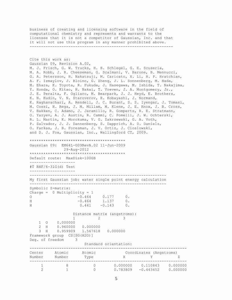
This is how the output file h2o.log looks like:
Entering Gaussian System, Link 0=g09
Input=h2o.com
Output=h2o.log
Initial command:
/gaussian/g09/l1.exe /gaussian/scratch/Gau-23178.inp -
scrdir=/gaussian/scratch/
Entering Link 1 = /gaussian/g09/l1.exe PID= 23179.
Copyright (c) 1988,1990,1992,1993,1995,1998,2003,2009, Gaussian, Inc.
All Rights Reserved.
This is part of the Gaussian(R) 09 program. It is based on
the Gaussian(R) 03 system (copyright 2003, Gaussian, Inc.),
the Gaussian(R) 98 system (copyright 1998, Gaussian, Inc.),
the Gaussian(R) 94 system (copyright 1995, Gaussian, Inc.),
the Gaussian 92(TM) system (copyright 1992, Gaussian, Inc.),
the Gaussian 90(TM) system (copyright 1990, Gaussian, Inc.),
the Gaussian 88(TM) system (copyright 1988, Gaussian, Inc.),
the Gaussian 86(TM) system (copyright 1986, Carnegie Mellon
University), and the Gaussian 82(TM) system (copyright 1983,
Carnegie Mellon University). Gaussian is a federally registered
trademark of Gaussian, Inc.
This software contains proprietary and confidential information,
including trade secrets, belonging to Gaussian, Inc.
This software is provided under written license and may be
used, copied, transmitted, or stored only in accord with that
written license.
The following legend is applicable only to US Government
contracts under FAR:
RESTRICTED RIGHTS LEGEND
Use, reproduction and disclosure by the US Government is
subject to restrictions as set forth in subparagraphs (a)
and (c) of the Commercial Computer Software - Restricted
Rights clause in FAR 52.227-19.
Gaussian, Inc.
340 Quinnipiac St., Bldg. 40, Wallingford CT 06492
---------------------------------------------------------------
Warning -- This program may not be used in any manner that
competes with the business of Gaussian, Inc. or will provide
assistance to any competitor of Gaussian, Inc. The licensee
of this program is prohibited from giving any competitor of
Gaussian, Inc. access to this program. By using this program,
the user acknowledges that Gaussian, Inc. is engaged in the
5
business of creating and licensing software in the field of
computational chemistry and represents and warrants to the
licensee that it is not a competitor of Gaussian, Inc. and that
it will not use this program in any manner prohibited above.
---------------------------------------------------------------
Cite this work as:
Gaussian 09, Revision A.02,
M. J. Frisch, G. W. Trucks, H. B. Schlegel, G. E. Scuseria,
M. A. Robb, J. R. Cheeseman, G. Scalmani, V. Barone, B. Mennucci,
G. A. Petersson, H. Nakatsuji, M. Caricato, X. Li, H. P. Hratchian,
A. F. Izmaylov, J. Bloino, G. Zheng, J. L. Sonnenberg, M. Hada,
M. Ehara, K. Toyota, R. Fukuda, J. Hasegawa, M. Ishida, T. Nakajima,
Y. Honda, O. Kitao, H. Nakai, T. Vreven, J. A. Montgomery, Jr.,
J. E. Peralta, F. Ogliaro, M. Bearpark, J. J. Heyd, E. Brothers,
K. N. Kudin, V. N. Staroverov, R. Kobayashi, J. Normand,
K. Raghavachari, A. Rendell, J. C. Burant, S. S. Iyengar, J. Tomasi,
M. Cossi, N. Rega, J. M. Millam, M. Klene, J. E. Knox, J. B. Cross,
V. Bakken, C. Adamo, J. Jaramillo, R. Gomperts, R. E. Stratmann,
O. Yazyev, A. J. Austin, R. Cammi, C. Pomelli, J. W. Ochterski,
R. L. Martin, K. Morokuma, V. G. Zakrzewski, G. A. Voth,
P. Salvador, J. J. Dannenberg, S. Dapprich, A. D. Daniels,
O. Farkas, J. B. Foresman, J. V. Ortiz, J. Cioslowski,
and D. J. Fox, Gaussian, Inc., Wallingford CT, 2009.
******************************************
Gaussian 09: EM64L-G09RevA.02 11-Jun-2009
29-Aug-2012
******************************************
Default route: MaxDisk=100GB
--------------------
#T RHF/6-31G(d) Test
--------------------
------------------------------------------------------------
My first Gaussian job: water single point energy calculation
------------------------------------------------------------
Symbolic Z-matrix:
Charge = 0 Multiplicity = 1
O -0.464 0.177 0.
H -0.464 1.137 0.
H 0.441 -0.143 0.
Distance matrix (angstroms):
1 2 3
1 O 0.000000
2 H 0.960000 0.000000
3 H 0.959909 1.567618 0.000000
Framework group CS[SG(H2O)]
Deg. of freedom 3
Standard orientation:
---------------------------------------------------------------------
Center Atomic Atomic Coordinates (Angstroms)
Number Number Type X Y Z
---------------------------------------------------------------------
1 8 0 0.000000 0.110843 0.000000
2 1 0 0.783809 -0.443452 0.000000

6
3 1 0 -0.783809 -0.443294 0.000000
---------------------------------------------------------------------
Rotational constants (GHZ): 919.1536408 408.1142629 282.6254666
19 basis functions, 36 primitive gaussians, 19 cartesian basis
functions
5 alpha electrons 5 beta electrons
nuclear repulsion energy 9.1576066717 Hartrees.
NAtoms= 3 NActive= 3 NUniq= 3 SFac= 7.50D-01 NAtFMM= 80 NAOKFM=F
Big=F
Harris functional with IExCor= 205 diagonalized for initial guess.
ExpMin= 1.61D-01 ExpMax= 5.48D+03 ExpMxC= 8.25D+02 IAcc=1 IRadAn= 1
AccDes= 0.00D+00
HarFok: IExCor= 205 AccDes= 0.00D+00 IRadAn= 1 IDoV= 1
ScaDFX= 1.000000 1.000000 1.000000 1.000000
FoFCou: FMM=F IPFlag= 0 FMFlag= 100000 FMFlg1= 0
NFxFlg= 0 DoJE=T BraDBF=F KetDBF=T FulRan=T
Omega= 0.000000 0.000000 1.000000 0.000000 0.000000 ICntrl=
500 IOpCl= 0
NMat0= 1 NMatS0= 1 NMatT0= 0 NMatD0= 1 NMtDS0= 0
NMtDT0= 0
I1Cent= 4 NGrid= 0.
Petite list used in FoFCou.
Initial guess orbital symmetries:
Occupied (A') (A') (A') (A') (A")
Virtual (A') (A') (A') (A') (A") (A') (A') (A') (A") (A')
(A") (A') (A') (A')
The electronic state of the initial guess is 1-A'.
SCF Done: E(RHF) = -76.0098709452 A.U. after 10 cycles
Convg = 0.4230D-08 -V/T = 2.0027
**********************************************************************
Population analysis using the SCF density.
**********************************************************************
Orbital symmetries:
Occupied (A') (A') (A') (A') (A")
Virtual (A') (A') (A') (A') (A') (A") (A') (A') (A") (A')
(A") (A') (A') (A')
The electronic state is 1-A'.
Alpha occ. eigenvalues -- -20.55794 -1.33616 -0.71421 -0.56030 -0.49560
Alpha virt. eigenvalues -- 0.21061 0.30391 1.04585 1.11668 1.15959
Alpha virt. eigenvalues -- 1.16928 1.38463 1.41676 2.03064 2.03552
Alpha virt. eigenvalues -- 2.07410 2.62759 2.94215 3.97815
Condensed to atoms (all electrons):
Mulliken atomic charges:
1
1 O -0.876158
2 H 0.438076
3 H 0.438082
Sum of Mulliken atomic charges = 0.00000
Mulliken charges with hydrogens summed into heavy atoms:
1
1 O 0.000000
Sum of Mulliken charges with hydrogens summed into heavy atoms = 0.00000
Electronic spatial extent (au): <R**2>= 18.9605

7
Charge= 0.0000 electrons
Dipole moment (field-independent basis, Debye):
X= -0.0001 Y= -2.1385 Z= 0.0000 Tot= 2.1385
Test job not archived.
1\1\ UNIVERSITY OF WYOMING, CHEMISTRY-BORN\SP\RHF\6-31G(d)\H2O1\JKUBEL
KA\29-Aug-2012\0\\#T RHF/6-31G(d) Test\\My first Gaussian job: water s
ingle point energy calculation\\0,1\O,0,-0.464,0.177,0.\H,0,-0.464,1.1
37,0.\H,0,0.441,-0.143,0.\\Version=EM64L-G09RevA.02\State=1-A'\HF=-76.
0098709\RMSD=4.230e-09\Dipole=0.6869663,0.4857774,0.\Quadrupole=0.2773
187,0.8269676,-1.1042863,-0.7769627,0.,0.\PG=CS [SG(H2O1)]\\@
LET US LEARN TO DREAM, GENTLEMEN, THEN PERHAPS WE SHALL
DISCOVER THE TRUTH; BUT LET US BEWARE OF PUBLISHING
OUR DREAMS ABROAD BEFORE THEY HAVE BEEN SCRUTINIZED
BY OUR VIGILANT INTELLECT ... LET US ALWAYS ALLOW
THE FRUIT TO HANG UNTIL IT IS RIPE. UNRIPE FRUIT
BRINGS EVEN THE GROWER BUT LITTLE PROFIT; IT DAMAGES
THE HEALTH OF THOSE WHO CONSUME IT; IT ENDANGERS
PARTICULARLY THE YOUTH WHO CANNOT YET DISTINGUISH
BETWEEN RIPE AND UNRIPE FRUIT.
-- KEKULE, 1890
Job cpu time: 0 days 0 hours 0 minutes 0.4 seconds.
File lengths (MBytes): RWF= 5 Int= 0 D2E= 0 Chk= 1 Scr= 1
Normal termination of Gaussian 09 at Wed Aug 29 08:54:03 2012.
The output file obviously contains a lot of information, usually a lot more than you need. It is
therefore important to know what you are looking for and to be able to locate the relevant
quantities. For example, the energy is always displayed as:
SCF Done: E(RHF) = -76.0098709452 A.U. after 10 cycles
You can also find it in the archive entry near the end, which summarizes all the results:
1\1\ UNIVERSITY OF WYOMING, CHEMISTRY-BORN\SP\RHF\6-31G(d)\H2O1\JKUBEL
KA\29-Aug-2012\0\\#T RHF/6-31G(d) Test\\My first Gaussian job: water s
ingle point energy calculation\\0,1\O,0,-0.464,0.177,0.\H,0,-0.464,1.1
37,0.\H,0,0.441,-0.143,0.\\Version=EM64L-G09RevA.02\State=1-A'\HF=-76.
0098709\RMSD=4.230e-09\Dipole=0.6869663,0.4857774,0.\Quadrupole=0.2773 187,0.8269676,-1.1042863,-0.7769627,0.,0.\PG=CS [SG(H2O1)]\\@
Be aware of units!
8
2.2. Gaussian input
Gaussian input is designed to be free-format and extremely flexible. For example, it is not case-
sensitive, and keywords and options may be shortened to a unique abbreviation. Detailed
description can be found on the Gaussian manual pages http://www.gaussian.com/g_tech/g_ur/
g09help.htm.
Gaussian input has the following basic structure. Input sections marked with an asterisk are
required in every input file.
Input Section Contents
Link 0 Commands Defines the locations of scratch files and job resource limits.
*Route Section Specifies the job type and model chemistry.
*blank line Separates the route section from the title section.
*Title Section Describes the job for the output and archive entry. *blank line
*Molecule Specification Gives the structure of the molecule to be studied. *blank line
Variables Section Specifies values for the variables used in the molecule specification. blank line
Separate input sections are separated from one another by blank lines. Note that some job types
may require additional sections not listed.
The Route Section
The first line of the route section always begins with a pound sign (#) in the first column. This
section specifies the theoretical procedure, basis set, and desired type of calculation. It may also
include other keywords. The ordering of keywords is not important. Exhaustive list of keywords
is found on Gaussian web pages http://www.gaussian.com/g_tech/g_ur/l_keywords09.htm
Some keywords require options; the following input line illustrates the possible formats for
keywords with options:
#T RHP/6-31G(d) SCF=Tight Units=(Bohr,Radian) Opt Test
Keyword with: a single option 2 options no options
The amount of spacing between items is not significant in Gaussian input. In the route section,
commas may be substituted for spaces if desired.
The route section may extend over more than one line if necessary. Only the first line need begin
with a pound sign, although any others may. The route section is terminated by a blank line.
The Title Section
The title section consists of one or more lines of descriptive information about the job. It is included
in the output and in the archive entry but is not otherwise used by Gaussian. It is terminated by a
blank line.
9
Specifying Molecular Structures
Gaussian accepts molecule specifications in several different formats:
Cartesian coordinates
Z-matrix format (internal coordinates)
Mixed internal and Cartesian coordinates
All molecule specifications require that the charge and spin multiplicity be specified (as two
integers) on the first line of this section. The charge is a positive or negative integer specifying the
total charge on the molecule. Thus, 1 or + 1 would be used for a singly-charged cation, -1
designates a singly-charged anion, and 0 represents a neutral molecule.
Spin Multiplicity
The spin multiplicity is given by the equation 2S + 1, where S is the total spin for the molecule.
Paired electrons contribute nothing to this quantity. They have a net spin of zero since an alpha
electron has a spin of +1/2 and a beta electron has a spin of -1/2 . Each unpaired electron
contributes +1/2 to S. Thus, a singlet - a system with no unpaired electrons - has a spin multiplicity
of 1, a doublet (one unpaired electron) has a spin multiplicity of 2, a triplet (two unpaired electrons
of like spin) has a spin multiplicity of 3, and so on.
Units
The units in a Z-matrix are Angstroms for lengths and degrees for angles by default; the default
units for Cartesian coordinates are Angstroms. These are also the default units for lengths and
angles used in Gaussian output. You can change them to Bohrs and/or radians by including the
Units keyword in the route section with one or both of its options: Bohr and Radian.
Cartesian Coordinate Input
Cartesian coordinate input consists of a series of lines of the form:
Atomic-symbol X-coordinate Y-coordinate Z-coordinate
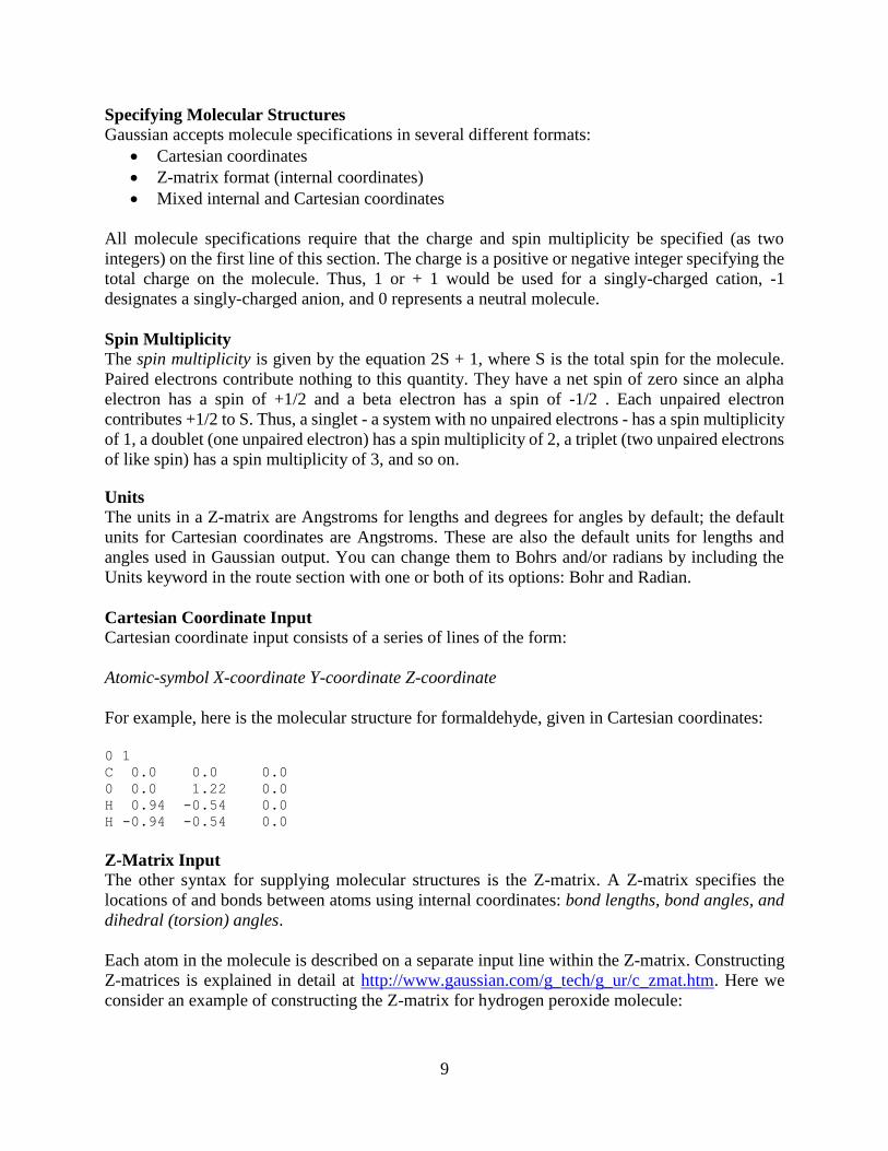
For example, here is the molecular structure for formaldehyde, given in Cartesian coordinates:
0 1
C 0.0 0.0 0.0
0 0.0 1.22 0.0
H 0.94 -0.54 0.0
H -0.94 -0.54 0.0
Z-Matrix Input
The other syntax for supplying molecular structures is the Z-matrix. A Z-matrix specifies the
locations of and bonds between atoms using internal coordinates: bond lengths, bond angles, and
dihedral (torsion) angles.
Each atom in the molecule is described on a separate input line within the Z-matrix. Constructing
Z-matrices is explained in detail at http://www.gaussian.com/g_tech/g_ur/c_zmat.htm. Here we
consider an example of constructing the Z-matrix for hydrogen peroxide molecule:
10
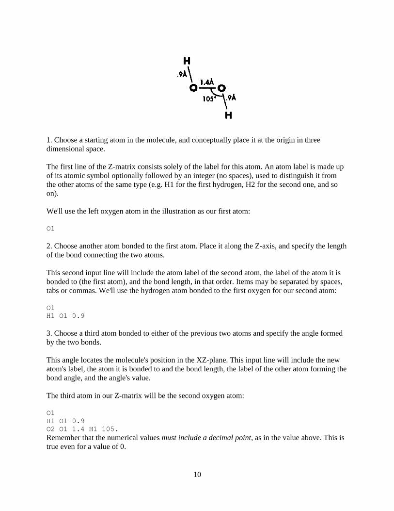
1. Choose a starting atom in the molecule, and conceptually place it at the origin in three
dimensional space.
The first line of the Z-matrix consists solely of the label for this atom. An atom label is made up
of its atomic symbol optionally followed by an integer (no spaces), used to distinguish it from
the other atoms of the same type (e.g. H1 for the first hydrogen, H2 for the second one, and so
on).
We'll use the left oxygen atom in the illustration as our first atom:
O1
2. Choose another atom bonded to the first atom. Place it along the Z-axis, and specify the length
of the bond connecting the two atoms.
This second input line will include the atom label of the second atom, the label of the atom it is
bonded to (the first atom), and the bond length, in that order. Items may be separated by spaces,
tabs or commas. We'll use the hydrogen atom bonded to the first oxygen for our second atom:
O1
H1 O1 0.9
3. Choose a third atom bonded to either of the previous two atoms and specify the angle formed
by the two bonds.
This angle locates the molecule's position in the XZ-plane. This input line will include the new
atom's label, the atom it is bonded to and the bond length, the label of the other atom forming the
bond angle, and the angle's value.
The third atom in our Z-matrix will be the second oxygen atom:
O1
H1 O1 0.9
O2 O1 1.4 H1 105.
Remember that the numerical values must include a decimal point, as in the value above. This is
true even for a value of 0.

11
4. Describe the positions of all subsequent atoms by specifying:
• Its atom label.
• An atom it is bonded to and the bond length.
• A third atom bonded to it (or to the second atom), and the value of the resulting bond
angle.
• A fourth atom bonded to either end of the previous chain, and the value of the dihedral
(torsion) angle formed by the four atoms.
Dihedral angles describe the angle the fourth atom makes with respect to the plane defined by the
first three atoms; their values range from 0 to 360 degrees, or from -180 to 180 degrees. Dihedral
angles are easy to visualize using Newman projections. The illustration shows the Newman
projection for hydrogen peroxide, looking down the O-O bond. Positive dihedral angles
correspond to clockwise rotation in the Newman projection.
The last atom to be specified is the second hydrogen. Here is the completed Z-matrix for
hydrogen peroxide:
0 1 Charge and multiplicity. O1 Oxygen atom #1.
Hl O1 0.9 Hydrogen #1, connected to oxygen #1 by a bond of 0.9 A.
O2 O1 1.4 Hl 105. Oxygen #2: O2-O1 = 1.4A: H1- O1-O2= 105°. H2 O2 0.9 O1 105. H1 120. Hydrogen #2: H2-O2 bond=0.9A: H2-O1-02 = 105°;
dihedral angle H2-O2-O1-H1 = 120°.
Using Variables in a Z-matrix
This file introduces the concept of variables within the molecule specification.
0 1 . O1 Hl O1 B1 O2 O1 B2 Hl A1 H2 O2 B1 O1 A1 H1 T1
B1=0.9
B2=1.4
A1=105.
T1=120.
Variables are simply named constants: variable names are substituted for numerical values within
the Z-matrix, and the actual values are defined in a separate section following it. The two sections
12
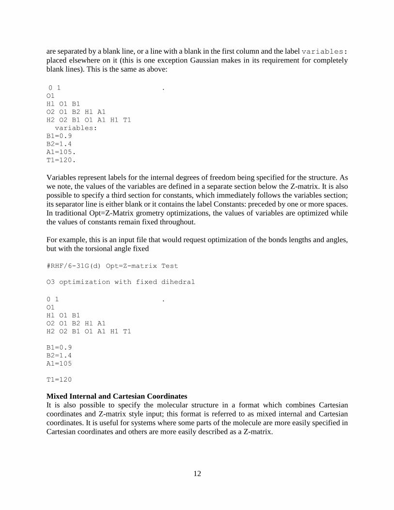
are separated by a blank line, or a line with a blank in the first column and the label variables:
placed elsewhere on it (this is one exception Gaussian makes in its requirement for completely
blank lines). This is the same as above:
0 1 . O1 Hl O1 B1 O2 O1 B2 Hl A1 H2 O2 B1 O1 A1 H1 T1
variables:
B1=0.9
B2=1.4
A1=105.
T1=120.
Variables represent labels for the internal degrees of freedom being specified for the structure. As
we note, the values of the variables are defined in a separate section below the Z-matrix. It is also
possible to specify a third section for constants, which immediately follows the variables section;
its separator line is either blank or it contains the label Constants: preceded by one or more spaces.
In traditional Opt=Z-Matrix grometry optimizations, the values of variables are optimized while
the values of constants remain fixed throughout.
For example, this is an input file that would request optimization of the bonds lengths and angles,
but with the torsional angle fixed
#RHF/6-31G(d) Opt=Z-matrix Test
O3 optimization with fixed dihedral
0 1 . O1 Hl O1 B1 O2 O1 B2 Hl A1 H2 O2 B1 O1 A1 H1 T1
B1=0.9
B2=1.4
A1=105
T1=120
Mixed Internal and Cartesian Coordinates
It is also possible to specify the molecular structure in a format which combines Cartesian
coordinates and Z-matrix style input; this format is referred to as mixed internal and Cartesian
coordinates. It is useful for systems where some parts of the molecule are more easily specified in
Cartesian coordinates and others are more easily described as a Z-matrix.

13
2.3. Building molecules with Gabedit
Obviously, it is not practical to generate input files manually for large and complex molecules. It
is much more convenient to build a molecule using some kind of a visual builder software, even
roughly optimize its structure if possible, and then save its coordinates. There are several free
programs available that can do this. We will use Gabedit, because it combines builder functionality
with viewing and animation of the results, which not many free programs out there can do.
Refer to Gabedit manual https://sites.google.com/site/allouchear/Home/gabedit/manual for
detailed description how to build molecules. Here we will do an example of N-methylacetamide.
I. Building the molecule
It is possible to draw molecules from scratch if necessary, using Insert/Change Atoms or Bonds
(the pencil symbol). Clicking generates an atom, clicking and dragging connects atoms by a
bond. Subsequent clicking on the middle of the bond changes it to a double bond, another click
to triple.
However, it is much better to start with a pre-optimized fragment. Load formamide from the
Fragment library (it can be found under Miscellaneous). It is always good to start with a
fragment, rather than generating the whole structure from scratch.
Click on Insert/Change Atoms or Bonds (the pencil symbol icon) and then on the Periodic table
icon and select Carbon. Click on the hydrogens you want to change to methyl groups. it is a good
idea to turn on number (right mouse click - Labels/Numbers) to make sure you really changed
only one atom and did not add more (with Gabedit all kinds of things can happen)
Select one of the methyl carbons by clicking on Selection of atoms icon and then dragging a
square around it. Then right click - Add/Max hydrogens will turn the carbon to a CH3 group.
Do the same for the other methyl group.
Clean (optimize) the structure. To do that, right click, select Set/Atom types using connection
types. Then right click again, select Molecular Mechanics/Optimization and click OK. Be
careful, the optimization does not always work right. Always examine the molecule and make
sure the structure is reasonable. In this case it should work.
Save the molecule (right click - Save As). It is always a good idea, in fact you may want to save
the intermediate steps during building just in case something happens so that you do not have to
start all over.
C
O
N
H
H3C
CH3
14
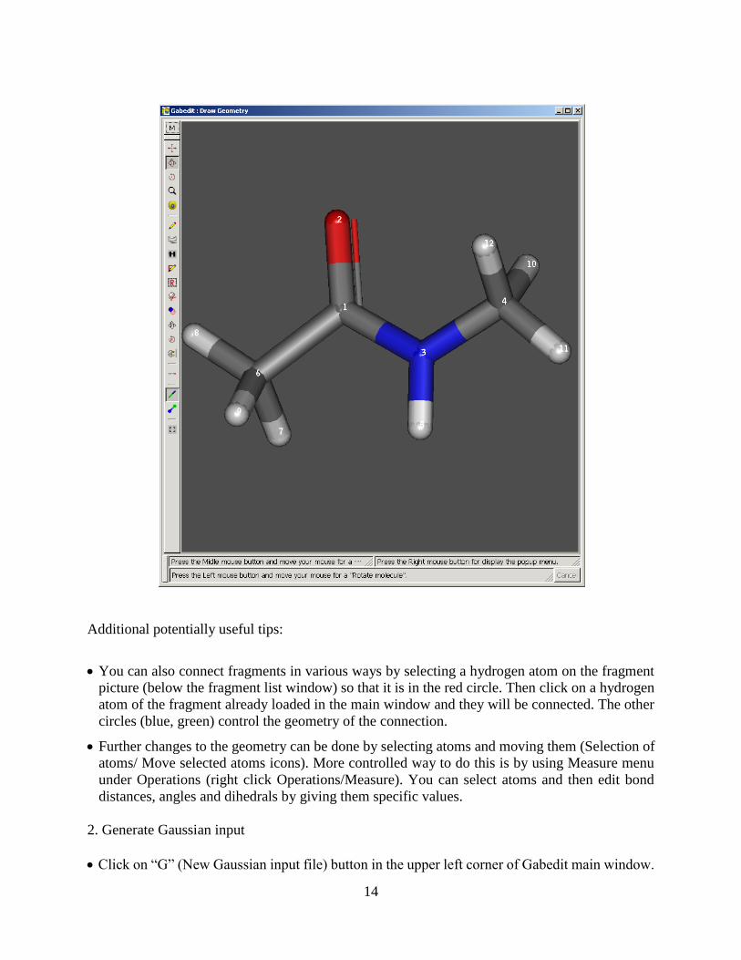
Additional potentially useful tips:
You can also connect fragments in various ways by selecting a hydrogen atom on the fragment
picture (below the fragment list window) so that it is in the red circle. Then click on a hydrogen
atom of the fragment already loaded in the main window and they will be connected. The other
circles (blue, green) control the geometry of the connection.
Further changes to the geometry can be done by selecting atoms and moving them (Selection of
atoms/ Move selected atoms icons). More controlled way to do this is by using Measure menu
under Operations (right click Operations/Measure). You can select atoms and then edit bond
distances, angles and dihedrals by giving them specific values.
2. Generate Gaussian input
Click on “G” (New Gaussian input file) button in the upper left corner of Gabedit main window.
15
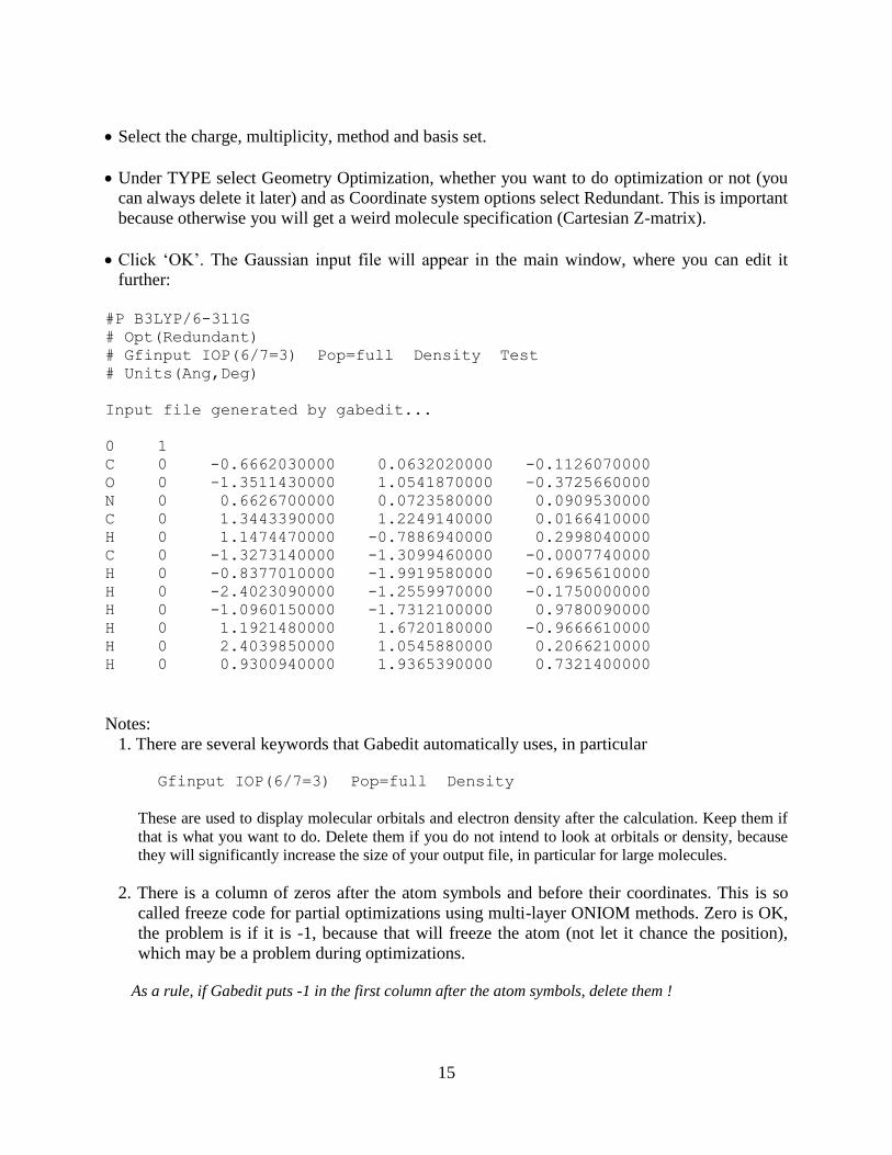
Select the charge, multiplicity, method and basis set.
Under TYPE select Geometry Optimization, whether you want to do optimization or not (you
can always delete it later) and as Coordinate system options select Redundant. This is important
because otherwise you will get a weird molecule specification (Cartesian Z-matrix).
Click ‘OK’. The Gaussian input file will appear in the main window, where you can edit it
further:
#P B3LYP/6-311G
# Opt(Redundant)
# Gfinput IOP(6/7=3) Pop=full Density Test
# Units(Ang,Deg)
Input file generated by gabedit...
0 1
C 0 -0.6662030000 0.0632020000 -0.1126070000
O 0 -1.3511430000 1.0541870000 -0.3725660000
N 0 0.6626700000 0.0723580000 0.0909530000
C 0 1.3443390000 1.2249140000 0.0166410000
H 0 1.1474470000 -0.7886940000 0.2998040000
C 0 -1.3273140000 -1.3099460000 -0.0007740000
H 0 -0.8377010000 -1.9919580000 -0.6965610000
H 0 -2.4023090000 -1.2559970000 -0.1750000000
H 0 -1.0960150000 -1.7312100000 0.9780090000
H 0 1.1921480000 1.6720180000 -0.9666610000
H 0 2.4039850000 1.0545880000 0.2066210000
H 0 0.9300940000 1.9365390000 0.7321400000
Notes:
1. There are several keywords that Gabedit automatically uses, in particular
Gfinput IOP(6/7=3) Pop=full Density
These are used to display molecular orbitals and electron density after the calculation. Keep them if
that is what you want to do. Delete them if you do not intend to look at orbitals or density, because
they will significantly increase the size of your output file, in particular for large molecules.
2. There is a column of zeros after the atom symbols and before their coordinates. This is so
called freeze code for partial optimizations using multi-layer ONIOM methods. Zero is OK,
the problem is if it is -1, because that will freeze the atom (not let it chance the position),
which may be a problem during optimizations.
As a rule, if Gabedit puts -1 in the first column after the atom symbols, delete them !
16
Edit the file at will. For example, if you do not want to optimize the structure and/or change
your mind about the method and basis set, want to add or delete keywords, change the title,
etc., just edit it in the Gabedit window.
Finally, save the file, e.g. as nma.com (File - Save As).
Now you can transfer the file and run Gaussian calculation.
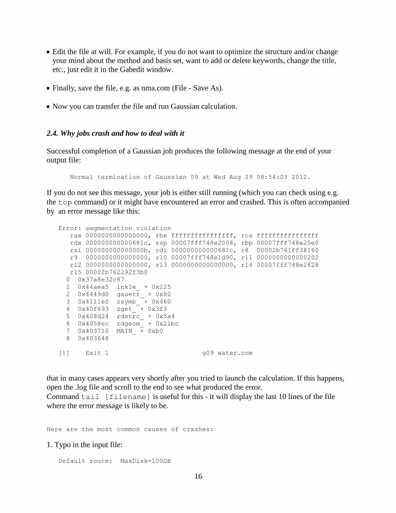
2.4. Why jobs crash and how to deal with it
Successful completion of a Gaussian job produces the following message at the end of your
output file:
Normal termination of Gaussian 09 at Wed Aug 29 08:54:03 2012.
If you do not see this message, your job is either still running (which you can check using e.g.
the top command) or it might have encountered an error and crashed. This is often accompanied
by an error message like this:
Error: segmentation violation
rax 0000000000000000, rbx ffffffffffffffff, rcx ffffffffffffffff
rdx 000000000000681c, rsp 00007fff748e2008, rbp 00007fff748e25e0
rsi 000000000000000b, rdi 000000000000681c, r8 00002b761ff38160
r9 0000000000000000, r10 00007fff748e1d90, r11 0000000000000202
r12 0000000000000000, r13 0000000000000000, r14 00007fff748e2628
r15 00002b762292f3b0
0 0x37a8e32c87
1 0x44aea5 lnk1e_ + 0x225
2 0x4449d0 gauerr_ + 0x80
3 0x4111e0 zsymb_ + 0x460
4 0x40f693 zget_ + 0x3f3
5 0x408d24 rdstrc_ + 0x5a4
6 0x4058ec rdgeom_ + 0x21bc
7 0x403710 MAIN_ + 0xb0
8 0x403648
[1] Exit 1 g09 water.com
that in many cases appears very shortly after you tried to launch the calculation. If this happens,
open the .log file and scroll to the end to see what produced the error.
Command tail [filename] is useful for this - it will display the last 10 lines of the file
where the error message is likely to be.
Here are the most common causes of crashes:
1. Typo in the input file:
Default route: MaxDisk=100GB

17
-------------------
#T RHF/6-31gd) test
-------------------
QPErr --- An ambiguous keyword was detected.
#T RHF/6-31gd) test
'
Last state="GCL"
TCursr= 486 LCursr= 12
Error termination via Lnk1e in /gaussian/g09/l1.exe at Wed Aug 29
18:36:12 2012.
Job cpu time: 0 days 0 hours 0 minutes 0.0 seconds.
File lengths (MBytes): RWF= 5 Int= 0 D2E= 0 Chk= 1 Scr= 1
2. Missing blank line:
Symbolic Z-matrix:
Charge = 0 Multiplicity = 1
O -0.464 0.177 0.
H -0.464 1.137 0.
H 0.441 -0.143 0.
End of file in ZSymb.
Error termination via Lnk1e in /gaussian/g09/l101.exe at Wed Aug 29
18:34:58 2012.
Job cpu time: 0 days 0 hours 0 minutes 0.0 seconds.
File lengths (MBytes): RWF= 5 Int= 0 D2E= 0 Chk= 1 Scr= 1
3. Badly specified molecule: atoms too close together:
Symbolic Z-matrix:
Charge = 0 Multiplicity = 1
O -0.464 0.177 0.
H -0.464 1.137 0.
H -0.441 0.143 0.
Distance matrix (angstroms):
1 2 3
1 O 0.000000
2 H 0.960000 0.000000
3 H 0.041049 0.994266 0.000000
Small interatomic distances encountered: 3 1
Problem with the distance matrix.
Error termination via Lnk1e in /gaussian/g09/l202.exe at Wed Aug 29
18:38:06 2012.
Job cpu time: 0 days 0 hours 0 minutes 0.1 seconds.
4. Missing charge/multiplicity line
%chk=water.chk
Default route: MaxDisk=100GB
--------------------
#T RHF/6-31g(d) test
--------------------

18
--------------
blah blah blah
--------------
Symbolic Z-matrix:
Charge and multiplicity card seems defective:
Charge is bogus.
WANTED AN INTEGER AS INPUT.
FOUND A STRING AS INPUT.
O -0.464 0.177 0.0
5. Wrong charge and/or multiplicity
The combination of multiplicity 1 and 9 electrons is impossible.
Error termination via Lnk1e in /gaussian/g09/l301.exe at Wed Aug 29
18:42:17 2012.
Job cpu time: 0 days 0 hours 0 minutes 0.1 seconds.
File lengths (MBytes): RWF= 5 Int= 0 D2E= 0 Chk= 1 Scr= 1
Careful: the fact that your job does not crash does not necessarily mean that spin and multiplicity
are correct - it only means that they make sense.
6. Failure of Self-Consistent Field (SCF) to converge. This could have many reasons, but in
99.99% cases it is due to bad molecular geometry:
Matrix for removal 18 Erem= -75.1396938671449 Crem= 0.000D+00
Matrix for removal 18 Erem= -75.1396938651034 Crem= 0.000D+00
Matrix for removal 9 Erem= -75.1396938680091 Crem= 0.000D+00
Rare condition: small coef for last iteration: 0.000D+00
Matrix for removal 18 Erem= -75.1396938595436 Crem= 0.000D+00
Matrix for removal 19 Erem= -75.1396938560966 Crem= 0.000D+00
Density matrix is not changing but DIIS error= 9.09D-02 CofLast= 0.00D+00.
>>>>>>>>>> Convergence criterion not met.
SCF Done: E(RHF) = -75.0970895430 A.U. after 129 cycles
Convg = 0.2526D-02 -V/T = 1.9726
Convergence failure -- run terminated.
Error termination via Lnk1e in /gaussian/g09/l502.exe at Wed Aug 29
18:40:15 2012.
Job cpu time: 0 days 0 hours 0 minutes 0.4 seconds.
File lengths (MBytes): RWF= 5 Int= 0 D2E= 0 Chk= 1 Scr= 1
In this case the starting H2O coordinates were completely wrong. Check (display) the starting
structure and make sure it’s OK.

19
2.5. Output of single point energy calculations
A single point energy calculation is a prediction of the energy and related properties for a molecule
with a specified geometric structure. The energy here is the sum of the electronic energy and
nuclear repulsion energy of the molecule at the specified nuclear configuration. This quantity is
commonly referred to as the total energy. However, more complete and accurate energy
predictions require a thermal or zero-point energy (ZPE) correction. We will get to that later.
The phrase single point means that the calculations is performed a single, fixed point on the
potential energy surface (PES) for the molecule. PES will be explored in the next chapter. The
validity of results of these calculations depends on having reasonable structures for the molecules
as input.
Single point energy calculations are performed for many purposes, including the following:
• To obtain basic information about a molecule.
• As a consistency check on a molecular geometry to be used as the starting point for an
optimization.
• To compute very accurate values for the energy and other properties for a geometry optimized
at a lower level of theory.
In addition to energy, the properties computed in single point energy calculations are:
• Molecular orbitals and electron density
• Dipole and higher multipole moments
• Atomic partial charges
• Other properties can be calculated as well using appropriate keywords, e.g. NMR shielding and
coupling constants, polarizabilities, hyperfine coupling constants etc.
As an example, we will consider a single point energy calculation for formaldehyde, using the
following input file:
#T RHF/6-31G(d) SCF=Tight Pop=Full Test
Formaldehyde Single Point
0 1
C 0.0 0.0 0.0
O 0.0 1.22 0.0
H 0.94 -0.54 0.0
H -0.94 -0.54 0.0
In this input SCF=Tight requests that the wavefunction convergence criteria be made more
stringent. The default criteria for single point energy calculations are generally accurate enough
for comparing the energies of similar molecules and for predicting properties such as molecular
orbitals and the dipole moment. SCF=VeryTight can be used to compute the energy using even
tighter SCF convergence criteria.
20
Pop=Full requests that all orbitals are displayed. If Pop=Reg was used instead, only five
highest occupied and five lowest virtual (empty) orbitals would be displayed.
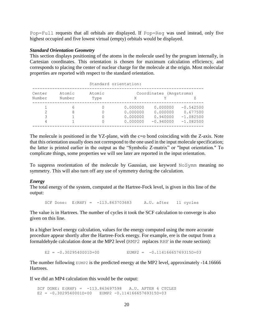
Standard Orientation Geometry
This section displays positioning of the atoms in the molecule used by the program internally, in
Cartesian coordinates. This orientation is chosen for maximum calculation efficiency, and
corresponds to placing the center of nuclear charge for the molecule at the origin. Most molecular
properties are reported with respect to the standard orientation.
Standard orientation:
---------------------------------------------------------------------
Center Atomic Atomic Coordinates (Angstroms)
Number Number Type X Y Z
---------------------------------------------------------------------
1 6 0 0.000000 0.000000 -0.542500
2 8 0 0.000000 0.000000 0.677500
3 1 0 0.000000 0.940000 -1.082500
4 1 0 0.000000 -0.940000 -1.082500
---------------------------------------------------------------------
The molecule is positioned in the YZ-plane, with the c=o bond coinciding with the Z-axis. Note
that this orientation usually does not correspond to the one used in the input molecule specification;
the latter is printed earlier in the output as the “Symbolic Z-matrix” or "Input orientation." To
complicate things, some properties we will see later are reported in the input orientation.
To suppress reorientation of the molecule by Gaussian, use keyword NoSymm meaning no
symmetry. This will also turn off any use of symmetry during the calculation.
Energy
The total energy of the system, computed at the Hartree-Fock level, is given in this line of the
output:
SCF Done: E(RHF) = -113.863703683 A.U. after 11 cycles
The value is in Hartrees. The number of cycles it took the SCF calculation to converge is also
given on this line.
In a higher level energy calculation, values for the energy computed using the more accurate
procedure appear shortly after the Hartree-Fock energy. For example, ere is the output from a
formaldehyde calculation done at the MP2 level (RMP2 replaces RHF in the route section):
E2 = -0.3029540001D+00 EUMP2 = -0.11416665769315D+03
The number following EUMP2 is the predicted energy at the MP2 level, approximately -14.16666
Hartrees.
If we did an MP4 calculation this would be the output:
SCF DONE: E(RHF) = -113.863697598 A.U. AFTER 6 CYCLES
E2 = -0.3029540001D+00 EUMP2 -0.11416665769315D+03
21
E3= -0.25563412D-02 EUMP3= -0.1141669850323D+03
E4(DQ)= -0.13383605D-02 UMP4(DQ)= -0.1141669872345D+03
E4(SDQ)= -0.31707330D-02 UMP4(SDQ)= -0.1141678953224D+03
E4(SDTQ)= -0.10020409D-01 UMP4(SDTQ)= -0.114168745328D+03
Notice that the energies for all of the lower-level methods-HF, MP2, MP3, MP4(DQ) and
MP4(SDQ)-are also given in a full MP4(SDTQ) calculation. That means if we wanted to compare
these different levels, we only need to do one calculation, not six.
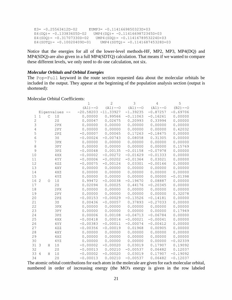
Molecular Orbitals and Orbital Energies
The Pop=Full keyword in the route section requested data about the molecular orbitals be
included in the output. They appear at the beginning of the population analysis section (output is
shortened):
Molecular Orbital Coefficients: 1 2 3 4 5 (A1)--O (A1)--O (A1)--O (A1)--O (B2)--O
Eigenvalues -- -20.58203 -11.33927 -1.39235 -0.87257 -0.69706
1 1 C 1S 0.00000 0.99566 -0.11063 -0.16261 0.00000
2 2S 0.00047 0.02675 0.20993 0.33994 0.00000
3 2PX 0.00000 0.00000 0.00000 0.00000 0.00000
4 2PY 0.00000 0.00000 0.00000 0.00000 0.42032
5 2PZ -0.00007 0.00065 0.17263 -0.18475 0.00000
6 3S -0.00024 -0.00743 0.08058 0.31305 0.00000
7 3PX 0.00000 0.00000 0.00000 0.00000 0.00000
8 3PY 0.00000 0.00000 0.00000 0.00000 0.15769
9 3PZ -0.00048 0.00135 -0.01158 -0.07978 0.00000
10 4XX -0.00002 -0.00272 -0.01629 -0.01333 0.00000
11 4YY -0.00006 -0.00202 -0.01364 0.03021 0.00000
12 4ZZ -0.00075 -0.00124 0.03301 -0.00166 0.00000
13 4XY 0.00000 0.00000 0.00000 0.00000 0.00000
14 4XZ 0.00000 0.00000 0.00000 0.00000 0.00000
15 4YZ 0.00000 0.00000 0.00000 0.00000 -0.01398
16 2 O 1S 0.99472 -0.00038 -0.19670 0.08887 0.00000
17 2S 0.02094 0.00025 0.44176 -0.20345 0.00000
18 2PX 0.00000 0.00000 0.00000 0.00000 0.00000
19 2PY 0.00000 0.00000 0.00000 0.00000 0.32078
20 2PZ -0.00153 -0.00029 -0.13526 -0.14181 0.00000
21 3S 0.00436 -0.00057 0.37893 -0.27033 0.00000
22 3PX 0.00000 0.00000 0.00000 0.00000 0.00000
23 3PY 0.00000 0.00000 0.00000 0.00000 0.17949
24 3PZ 0.00006 0.00108 -0.04713 -0.06784 0.00000
25 4XX -0.00418 0.00014 -0.00021 -0.00041 0.00000
26 4YY -0.00383 -0.00011 -0.00074 -0.00412 0.00000
27 4ZZ -0.00356 -0.00019 0.01968 0.00905 0.00000
28 4XY 0.00000 0.00000 0.00000 0.00000 0.00000
29 4XZ 0.00000 0.00000 0.00000 0.00000 0.00000
30 4YZ 0.00000 0.00000 0.00000 0.00000 -0.02339
31 3 H 1S -0.00002 -0.00020 0.03019 0.17907 0.19092
32 2S -0.00013 0.00210 -0.00537 0.06482 0.12037
33 4 H 1S -0.00002 -0.00020 0.03019 0.17907 -0.19092
34 2S -0.00013 0.00210 -0.00537 0.06482 -0.12037
The atomic orbital contributions for each atom in the molecule are given for each molecular orbital,
numbered in order of increasing energy (the MO's energy is given in the row labeled
22
EIGENVALUES preceding the orbital coefficients). The symmetry of the orbital and whether it is
an occupied orbital or a virtual (unoccupied) orbital appears immediately under the orbital number.
When comparing orbital coefficients, most important are their relative magnitudes with respect to
one another within that orbital (regardless of sign). For example, for the first-lowest energy-
molecular orbital, the carbon 2s and 2pz' the oxygen 1s, 2s, and 2pz and the 1s orbitals on both
hydrogens all have non-zero coefficients. However, the magnitude of the 1s coefficient on the
oxygen is much larger than all the others: therefore this molecular orbital essentially corresponds
to the oxygen 1s orbital. Similarly, the important component for the second molecular orbital is
the 1s orbital from the carbon atom.
The highest occupied molecular orbital (HOMO) and lowest unoccupied molecular orbital
(LUMO) may be identified by finding the point where the occupied/virtual code letter in the
symmetry designation changes from O to V. Here are the energies and symmetry designations for
the next set of molecular orbitals for formaldehyde:
6 7 8 9 10
(A1)--O (B1)--O (B2)--O (B1)--V (A1)--V
Eigenvalues -- -0.63916 -0.52290 -0.44043 0.13577 0.24838
1 1 C 1S 0.01957 0.00000 0.00000 0.00000 -0.12210
2 2S -0.06111 0.00000 0.00000 0.00000 0.14892
For formaldehyde, molecular orbital number 8 is the HOMO, and molecular orbital number 9 is
the LUMO. In this case, the energy also changes sign at the point separating the occupied from
the unoccupied orbitals.
We will see how the molecular orbitals can be visualized with Gabedit. Chemists love orbitals and
they are important in illustrating and explaining many chemistry concepts, such as bonding and
reactivity. However, it is important to remember that orbitals are only convenient abstract
mathematical constructs and not real physical observables.
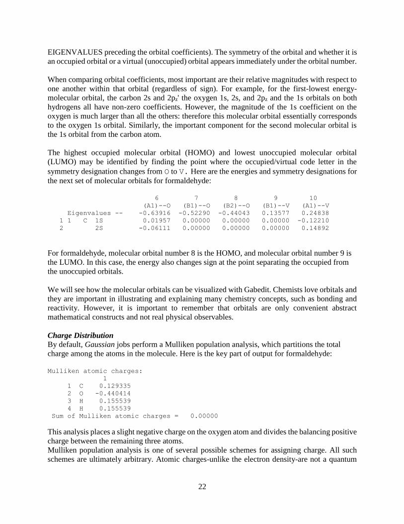
Charge Distribution
By default, Gaussian jobs perform a Mulliken population analysis, which partitions the total
charge among the atoms in the molecule. Here is the key part of output for formaldehyde:
Mulliken atomic charges:
1
1 C 0.129335
2 O -0.440414
3 H 0.155539
4 H 0.155539
Sum of Mulliken atomic charges = 0.00000
This analysis places a slight negative charge on the oxygen atom and divides the balancing positive
charge between the remaining three atoms.
Mulliken population analysis is one of several possible schemes for assigning charge. All such
schemes are ultimately arbitrary. Atomic charges-unlike the electron density-are not a quantum
23
mechanical observable, and are not unambiguously predictable from first principles. Other
methods for assigning charges to atoms will be explored later.
Dipole and Higher Multipole Moments
Gaussian also predicts dipole moments and higher multipole moments (through hexadecapole).
The dipole moment is the first derivative of the energy with respect to an applied electric field. It
is a measure of the asymmetry in the molecular charge distribution, and is given as a vector in
three dimensions. For Hartree-Fock calculations, this is equivalent to the expectation value of X,
Y, and Z, which are the quantities reported in the output.
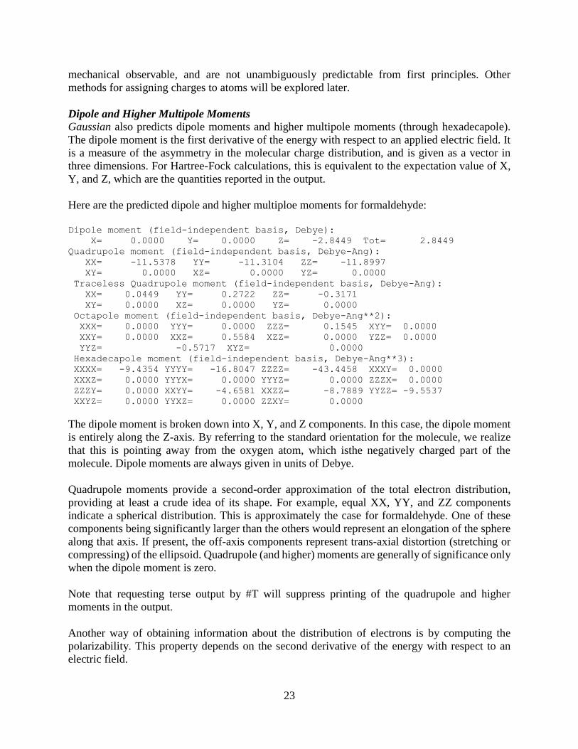
Here are the predicted dipole and higher multiploe moments for formaldehyde:
Dipole moment (field-independent basis, Debye):
X= 0.0000 Y= 0.0000 Z= -2.8449 Tot= 2.8449
Quadrupole moment (field-independent basis, Debye-Ang):
XX= -11.5378 YY= -11.3104 ZZ= -11.8997
XY= 0.0000 XZ= 0.0000 YZ= 0.0000
Traceless Quadrupole moment (field-independent basis, Debye-Ang):
XX= 0.0449 YY= 0.2722 ZZ= -0.3171
XY= 0.0000 XZ= 0.0000 YZ= 0.0000
Octapole moment (field-independent basis, Debye-Ang**2):
XXX= 0.0000 YYY= 0.0000 ZZZ= 0.1545 XYY= 0.0000
XXY= 0.0000 XXZ= 0.5584 XZZ= 0.0000 YZZ= 0.0000
YYZ= -0.5717 XYZ= 0.0000
Hexadecapole moment (field-independent basis, Debye-Ang**3):
XXXX= -9.4354 YYYY= -16.8047 ZZZZ= -43.4458 XXXY= 0.0000
XXXZ= 0.0000 YYYX= 0.0000 YYYZ= 0.0000 ZZZX= 0.0000
ZZZY= 0.0000 XXYY= -4.6581 XXZZ= -8.7889 YYZZ= -9.5537
XXYZ= 0.0000 YYXZ= 0.0000 ZZXY= 0.0000
The dipole moment is broken down into X, Y, and Z components. In this case, the dipole moment
is entirely along the Z-axis. By referring to the standard orientation for the molecule, we realize
that this is pointing away from the oxygen atom, which isthe negatively charged part of the
molecule. Dipole moments are always given in units of Debye.
Quadrupole moments provide a second-order approximation of the total electron distribution,
providing at least a crude idea of its shape. For example, equal XX, YY, and ZZ components
indicate a spherical distribution. This is approximately the case for formaldehyde. One of these
components being significantly larger than the others would represent an elongation of the sphere
along that axis. If present, the off-axis components represent trans-axial distortion (stretching or
compressing) of the ellipsoid. Quadrupole (and higher) moments are generally of significance only
when the dipole moment is zero.
Note that requesting terse output by #T will suppress printing of the quadrupole and higher
moments in the output.
Another way of obtaining information about the distribution of electrons is by computing the
polarizability. This property depends on the second derivative of the energy with respect to an
electric field.
24
CPU Time and Other Resource Usage
Gaussian jobs report the CPU time used and the sizes of their scratch files upon completion.
Here is the data for our formaldehyde job:
Job cpu time: 0 days 0 hours 0 minutes 0.4 seconds.
File lengths (MBytes): RWF= 5 Int= 0 D2E= 0 Chk= 1 Scr= 1
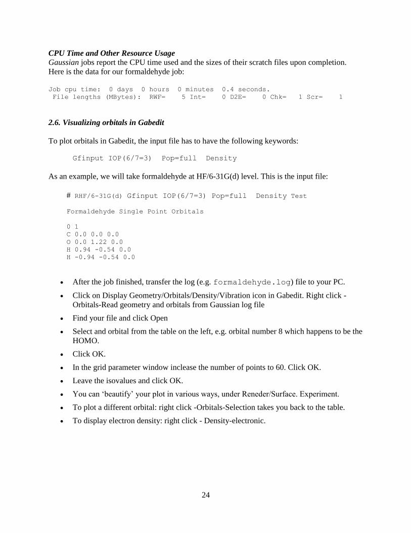
2.6. Visualizing orbitals in Gabedit
To plot orbitals in Gabedit, the input file has to have the following keywords:
Gfinput IOP(6/7=3) Pop=full Density
As an example, we will take formaldehyde at HF/6-31G(d) level. This is the input file:
# RHF/6-31G(d) Gfinput IOP(6/7=3) Pop=full Density Test
Formaldehyde Single Point Orbitals
0 1
C 0.0 0.0 0.0
O 0.0 1.22 0.0
H 0.94 -0.54 0.0
H -0.94 -0.54 0.0
After the job finished, transfer the log (e.g. formaldehyde.log) file to your PC.
Click on Display Geometry/Orbitals/Density/Vibration icon in Gabedit. Right click -
Orbitals-Read geometry and orbitals from Gaussian log file
Find your file and click Open
Select and orbital from the table on the left, e.g. orbital number 8 which happens to be the
HOMO.
Click OK.
In the grid parameter window inclease the number of points to 60. Click OK.
Leave the isovalues and click OK.
You can ‘beautify’ your plot in various ways, under Reneder/Surface. Experiment.
To plot a different orbital: right click -Orbitals-Selection takes you back to the table.
To display electron density: right click - Density-electronic.