Part IA - Vectors and Matrices - Maths Lecture Notes IA | Vectors and Matrices Based on lectures by...
70
Part IA — Vectors and Matrices Based on lectures by N. Peake Notes taken by Dexter Chua Michaelmas 2014 These notes are not endorsed by the lecturers, and I have modified them (often significantly) after lectures. They are nowhere near accurate representations of what was actually lectured, and in particular, all errors are almost surely mine. Complex numbers Review of complex numbers, including complex conjugate, inverse, modulus, argument and Argand diagram. Informal treatment of complex logarithm, n-th roots and complex powers. de Moivre’s theorem. [2] Vectors Review of elementary algebra of vectors in R 3 , including scalar product. Brief discussion of vectors in R n and C n ; scalar product and the Cauchy-Schwarz inequality. Concepts of linear span, linear independence, subspaces, basis and dimension. Suffix notation: including summation convention, δij and ε ijk . Vector product and triple product: definition and geometrical interpretation. Solution of linear vector equations. Applications of vectors to geometry, including equations of lines, planes and spheres. [5] Matrices Elementary algebra of 3 × 3 matrices, including determinants. Extension to n × n complex matrices. Trace, determinant, non-singular matrices and inverses. Matrices as linear transformations; examples of geometrical actions including rotations, reflections, dilations, shears; kernel and image. [4] Simultaneous linear equations: matrix formulation; existence and uniqueness of solu- tions, geometric interpretation; Gaussian elimination. [3] Symmetric, anti-symmetric, orthogonal, hermitian and unitary matrices. Decomposition of a general matrix into isotropic, symmetric trace-free and antisymmetric parts. [1] Eigenvalues and Eigenvectors Eigenvalues and eigenvectors; geometric significance. [2] Proof that eigenvalues of hermitian matrix are real, and that distinct eigenvalues give an orthogonal basis of eigenvectors. The effect of a general change of basis (similarity transformations). Diagonalization of general matrices: sufficient conditions; examples of matrices that cannot be diagonalized. Canonical forms for 2 × 2 matrices. [5] Discussion of quadratic forms, including change of basis. Classification of conics, cartesian and polar forms. [1] Rotation matrices and Lorentz transformations as transformation groups. [1] 1
Transcript of Part IA - Vectors and Matrices - Maths Lecture Notes IA | Vectors and Matrices Based on lectures by...

Part IA — Vectors and Matrices
Based on lectures by N. PeakeNotes taken by Dexter Chua
Michaelmas 2014
These notes are not endorsed by the lecturers, and I have modified them (oftensignificantly) after lectures. They are nowhere near accurate representations of what
was actually lectured, and in particular, all errors are almost surely mine.
Complex numbersReview of complex numbers, including complex conjugate, inverse, modulus, argumentand Argand diagram. Informal treatment of complex logarithm, n-th roots and complexpowers. de Moivre’s theorem. [2]
VectorsReview of elementary algebra of vectors in R3, including scalar product. Brief discussionof vectors in Rn and Cn; scalar product and the Cauchy-Schwarz inequality. Conceptsof linear span, linear independence, subspaces, basis and dimension.
Suffix notation: including summation convention, δij and εijk. Vector product andtriple product: definition and geometrical interpretation. Solution of linear vectorequations. Applications of vectors to geometry, including equations of lines, planes andspheres. [5]
MatricesElementary algebra of 3 × 3 matrices, including determinants. Extension to n × ncomplex matrices. Trace, determinant, non-singular matrices and inverses. Matrices aslinear transformations; examples of geometrical actions including rotations, reflections,dilations, shears; kernel and image. [4]
Simultaneous linear equations: matrix formulation; existence and uniqueness of solu-tions, geometric interpretation; Gaussian elimination. [3]
Symmetric, anti-symmetric, orthogonal, hermitian and unitary matrices. Decompositionof a general matrix into isotropic, symmetric trace-free and antisymmetric parts. [1]
Eigenvalues and EigenvectorsEigenvalues and eigenvectors; geometric significance. [2]
Proof that eigenvalues of hermitian matrix are real, and that distinct eigenvalues givean orthogonal basis of eigenvectors. The effect of a general change of basis (similaritytransformations). Diagonalization of general matrices: sufficient conditions; examplesof matrices that cannot be diagonalized. Canonical forms for 2 × 2 matrices. [5]
Discussion of quadratic forms, including change of basis. Classification of conics,cartesian and polar forms. [1]
Rotation matrices and Lorentz transformations as transformation groups. [1]
1

Contents IA Vectors and Matrices
Contents
0 Introduction 4
1 Complex numbers 51.1 Basic properties . . . . . . . . . . . . . . . . . . . . . . . . . . . . 51.2 Complex exponential function . . . . . . . . . . . . . . . . . . . . 61.3 Roots of unity . . . . . . . . . . . . . . . . . . . . . . . . . . . . . 81.4 Complex logarithm and power . . . . . . . . . . . . . . . . . . . . 81.5 De Moivre’s theorem . . . . . . . . . . . . . . . . . . . . . . . . . 81.6 Lines and circles in C . . . . . . . . . . . . . . . . . . . . . . . . 9
2 Vectors 112.1 Definition and basic properties . . . . . . . . . . . . . . . . . . . 112.2 Scalar product . . . . . . . . . . . . . . . . . . . . . . . . . . . . 11
2.2.1 Geometric picture (R2 and R3 only) . . . . . . . . . . . . 122.2.2 General algebraic definition . . . . . . . . . . . . . . . . . 12
2.3 Cauchy-Schwarz inequality . . . . . . . . . . . . . . . . . . . . . . 132.4 Vector product . . . . . . . . . . . . . . . . . . . . . . . . . . . . 142.5 Scalar triple product . . . . . . . . . . . . . . . . . . . . . . . . . 142.6 Spanning sets and bases . . . . . . . . . . . . . . . . . . . . . . . 15
2.6.1 2D space . . . . . . . . . . . . . . . . . . . . . . . . . . . 152.6.2 3D space . . . . . . . . . . . . . . . . . . . . . . . . . . . 162.6.3 Rn space . . . . . . . . . . . . . . . . . . . . . . . . . . . 162.6.4 Cn space . . . . . . . . . . . . . . . . . . . . . . . . . . . 17
2.7 Vector subspaces . . . . . . . . . . . . . . . . . . . . . . . . . . . 172.8 Suffix notation . . . . . . . . . . . . . . . . . . . . . . . . . . . . 182.9 Geometry . . . . . . . . . . . . . . . . . . . . . . . . . . . . . . . 21
2.9.1 Lines . . . . . . . . . . . . . . . . . . . . . . . . . . . . . . 212.9.2 Plane . . . . . . . . . . . . . . . . . . . . . . . . . . . . . 22
2.10 Vector equations . . . . . . . . . . . . . . . . . . . . . . . . . . . 22
3 Linear maps 243.1 Examples . . . . . . . . . . . . . . . . . . . . . . . . . . . . . . . 24
3.1.1 Rotation in R3 . . . . . . . . . . . . . . . . . . . . . . . . 243.1.2 Reflection in R3 . . . . . . . . . . . . . . . . . . . . . . . 25
3.2 Linear Maps . . . . . . . . . . . . . . . . . . . . . . . . . . . . . . 253.3 Rank and nullity . . . . . . . . . . . . . . . . . . . . . . . . . . . 263.4 Matrices . . . . . . . . . . . . . . . . . . . . . . . . . . . . . . . . 27
3.4.1 Examples . . . . . . . . . . . . . . . . . . . . . . . . . . . 283.4.2 Matrix Algebra . . . . . . . . . . . . . . . . . . . . . . . . 293.4.3 Decomposition of an n× n matrix . . . . . . . . . . . . . 303.4.4 Matrix inverse . . . . . . . . . . . . . . . . . . . . . . . . 31
3.5 Determinants . . . . . . . . . . . . . . . . . . . . . . . . . . . . . 323.5.1 Permutations . . . . . . . . . . . . . . . . . . . . . . . . . 323.5.2 Properties of determinants . . . . . . . . . . . . . . . . . 333.5.3 Minors and Cofactors . . . . . . . . . . . . . . . . . . . . 35
2

Contents IA Vectors and Matrices
4 Matrices and linear equations 384.1 Simple example, 2× 2 . . . . . . . . . . . . . . . . . . . . . . . . 384.2 Inverse of an n× n matrix . . . . . . . . . . . . . . . . . . . . . . 384.3 Homogeneous and inhomogeneous equations . . . . . . . . . . . . 39
4.3.1 Gaussian elimination . . . . . . . . . . . . . . . . . . . . . 404.4 Matrix rank . . . . . . . . . . . . . . . . . . . . . . . . . . . . . . 424.5 Homogeneous problem Ax = 0 . . . . . . . . . . . . . . . . . . . 42
4.5.1 Geometrical interpretation . . . . . . . . . . . . . . . . . . 434.5.2 Linear mapping view of Ax = 0 . . . . . . . . . . . . . . . 43
4.6 General solution of Ax = d . . . . . . . . . . . . . . . . . . . . . 43
5 Eigenvalues and eigenvectors 465.1 Preliminaries and definitions . . . . . . . . . . . . . . . . . . . . . 465.2 Linearly independent eigenvectors . . . . . . . . . . . . . . . . . . 485.3 Transformation matrices . . . . . . . . . . . . . . . . . . . . . . . 50
5.3.1 Transformation law for vectors . . . . . . . . . . . . . . . 515.3.2 Transformation law for matrix . . . . . . . . . . . . . . . 52
5.4 Similar matrices . . . . . . . . . . . . . . . . . . . . . . . . . . . 535.5 Diagonalizable matrices . . . . . . . . . . . . . . . . . . . . . . . 545.6 Canonical (Jordan normal) form . . . . . . . . . . . . . . . . . . 555.7 Cayley-Hamilton Theorem . . . . . . . . . . . . . . . . . . . . . . 575.8 Eigenvalues and eigenvectors of a Hermitian matrix . . . . . . . . 58
5.8.1 Eigenvalues and eigenvectors . . . . . . . . . . . . . . . . 585.8.2 Gram-Schmidt orthogonalization (non-examinable) . . . . 595.8.3 Unitary transformation . . . . . . . . . . . . . . . . . . . 605.8.4 Diagonalization of n× n Hermitian matrices . . . . . . . 605.8.5 Normal matrices . . . . . . . . . . . . . . . . . . . . . . . 62
6 Quadratic forms and conics 636.1 Quadrics and conics . . . . . . . . . . . . . . . . . . . . . . . . . 63
6.1.1 Quadrics . . . . . . . . . . . . . . . . . . . . . . . . . . . 636.1.2 Conic sections (n = 2) . . . . . . . . . . . . . . . . . . . . 64
6.2 Focus-directrix property . . . . . . . . . . . . . . . . . . . . . . . 65
7 Transformation groups 687.1 Groups of orthogonal matrices . . . . . . . . . . . . . . . . . . . 687.2 Length preserving matrices . . . . . . . . . . . . . . . . . . . . . 687.3 Lorentz transformations . . . . . . . . . . . . . . . . . . . . . . . 69
3

0 Introduction IA Vectors and Matrices
0 Introduction
Vectors and matrices is the language in which a lot of mathematics is writtenin. In physics, many variables such as position and momentum are expressed asvectors. Heisenberg also formulated quantum mechanics in terms of vectors andmatrices. In statistics, one might pack all the results of all experiments into asingle vector, and work with a large vector instead of many small quantities. Ingroup theory, matrices are used to represent the symmetries of space (as well asmany other groups).
So what is a vector? Vectors are very general objects, and can in theoryrepresent very complex objects. However, in this course, our focus is on vectorsin Rn or Cn. We can think of each of these as an array of n real or complexnumbers. For example, (1, 6, 4) is a vector in R3. These vectors are added in theobvious way. For example, (1, 6, 4) + (3, 5, 2) = (4, 11, 6). We can also multiplyvectors by numbers, say 2(1, 6, 4) = (2, 12, 8). Often, these vectors representpoints in an n-dimensional space.
Matrices, on the other hand, represent functions between vectors, i.e. afunction that takes in a vector and outputs another vector. These, however, arenot arbitrary functions. Instead matrices represent linear functions. These arefunctions that satisfy the equality f(λx + µy) = λf(x) + µf(y) for arbitrarynumbers λ, µ and vectors x,y. It is important to note that the function x 7→ x+cfor some constant vector c is not linear according to this definition, even thoughit might look linear.
It turns out that for each linear function from Rn to Rm, we can representthe function uniquely by an m× n array of numbers, which is what we call thematrix. Expressing a linear function as a matrix allows us to conveniently studymany of its properties, which is why we usually talk about matrices instead ofthe function itself.
4

1 Complex numbers IA Vectors and Matrices
1 Complex numbers
In R, not every polynomial equation has a solution. For example, there doesnot exist any x such that x2 + 1 = 0, since for any x, x2 is non-negative, andx2 + 1 can never be 0. To solve this problem, we introduce the “number” i thatsatisfies i2 = −1. Then i is a solution to the equation x2 + 1 = 0. Similarly, −iis also a solution to the equation.
We can add and multiply numbers with i. For example, we can obtainnumbers 3 + i or 1 + 3i. These numbers are known as complex numbers. It turnsout that by adding this single number i, every polynomial equation will have aroot. In fact, for an nth order polynomial equation, we will later see that therewill always be n roots, if we account for multiplicity. We will go into details inChapter 5.
Apart from solving equations, complex numbers have a lot of rather importantapplications. For example, they are used in electronics to represent alternatingcurrents, and form an integral part in the formulation of quantum mechanics.
1.1 Basic properties
Definition (Complex number). A complex number is a number z ∈ C of theform z = a+ ib with a, b ∈ R, where i2 = −1. We write a = Re(z) and b = Im(z).
We have
z1 ± z2 = (a1 + ib1)± (a2 + ib2)
= (a1 ± a2) + i(b1 ± b2)
z1z2 = (a1 + ib1)(a2 + ib2)
= (a1a2 − b1b2) + i(b1a2 + a1b2)
z−1 =1
a+ ib
=a− iba2 + b2
Definition (Complex conjugate). The complex conjugate of z = a+ ib is a− ib.It is written as z or z∗.
It is often helpful to visualize complex numbers in a diagram:
Definition (Argand diagram). An Argand diagram is a diagram in which a
complex number z = x+ iy is represented by a vector p =
(xy
). Addition of
vectors corresponds to vector addition and z is the reflection of z in the x-axis.
Re
Im
z1z2
z2
z1 + z2
5
1 Complex numbers IA Vectors and Matrices
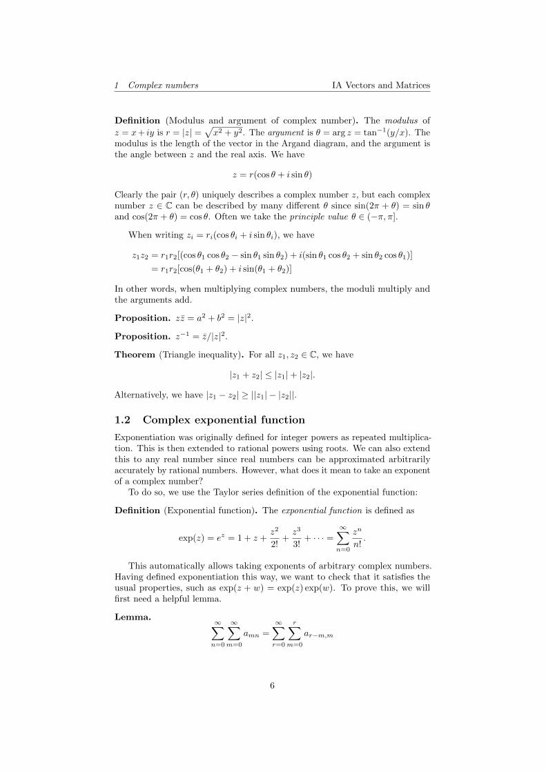
Definition (Modulus and argument of complex number). The modulus of
z = x+ iy is r = |z| =√x2 + y2. The argument is θ = arg z = tan−1(y/x). The
modulus is the length of the vector in the Argand diagram, and the argument isthe angle between z and the real axis. We have
z = r(cos θ + i sin θ)
Clearly the pair (r, θ) uniquely describes a complex number z, but each complexnumber z ∈ C can be described by many different θ since sin(2π + θ) = sin θand cos(2π + θ) = cos θ. Often we take the principle value θ ∈ (−π, π].
When writing zi = ri(cos θi + i sin θi), we have
z1z2 = r1r2[(cos θ1 cos θ2 − sin θ1 sin θ2) + i(sin θ1 cos θ2 + sin θ2 cos θ1)]
= r1r2[cos(θ1 + θ2) + i sin(θ1 + θ2)]
In other words, when multiplying complex numbers, the moduli multiply andthe arguments add.
Proposition. zz = a2 + b2 = |z|2.
Proposition. z−1 = z/|z|2.
Theorem (Triangle inequality). For all z1, z2 ∈ C, we have
|z1 + z2| ≤ |z1|+ |z2|.
Alternatively, we have |z1 − z2| ≥ ||z1| − |z2||.
1.2 Complex exponential function
Exponentiation was originally defined for integer powers as repeated multiplica-tion. This is then extended to rational powers using roots. We can also extendthis to any real number since real numbers can be approximated arbitrarilyaccurately by rational numbers. However, what does it mean to take an exponentof a complex number?
To do so, we use the Taylor series definition of the exponential function:
Definition (Exponential function). The exponential function is defined as
exp(z) = ez = 1 + z +z2
2!+z3
3!+ · · · =
∞∑n=0
zn
n!.
This automatically allows taking exponents of arbitrary complex numbers.Having defined exponentiation this way, we want to check that it satisfies theusual properties, such as exp(z + w) = exp(z) exp(w). To prove this, we willfirst need a helpful lemma.
Lemma.∞∑n=0
∞∑m=0
amn =
∞∑r=0
r∑m=0
ar−m,m
6

1 Complex numbers IA Vectors and Matrices
Proof.
∞∑n=0
∞∑m=0
amn = a00 + a01 + a02 + · · ·
+ a10 + a11 + a12 + · · ·+ a20 + a21 + a22 + · · ·= (a00) + (a10 + a01) + (a20 + a11 + a02) + · · ·
=
∞∑r=0
r∑m=0
ar−m,m
This is not exactly a rigorous proof, since we should not hand-wave aboutinfinite sums so casually. But in fact, we did not even show that the definition ofexp(z) is well defined for all numbers z, since the sum might diverge. All thesewill be done in that IA Analysis I course.
Theorem. exp(z1) exp(z2) = exp(z1 + z2)
Proof.
exp(z1) exp(z2) =
∞∑n=0
∞∑m=0
zm1m!
zn2n!
=
∞∑r=0
r∑m=0
zr−m1
(r −m)!
zm2m!
=
∞∑r=0
1
r!
r∑m=0
r!
(r −m)!m!zr−m1 zm2
=
∞∑r=0
(z1 + z2)r
r!
Again, to define the sine and cosine functions, instead of referring to “angles”(since it doesn’t make much sense to refer to complex “angles”), we again use aseries definition.
Definition (Sine and cosine functions). Define, for all z ∈ C,
sin z =
∞∑n=0
(−1)n
(2n+ 1)!z2n+1 = z − 1
3!z3 +
1
5!z5 + · · ·
cos z =
∞∑n=0
(−1)n
(2n)!z2n = 1− 1
2!z2 +
1
4!z4 + · · ·
One very important result is the relationship between exp, sin and cos.
Theorem. eiz = cos z + i sin z.
Alternatively, since sin(−z) = − sin z and cos(−z) = cos z, we have
cos z =eiz + e−iz
2,
sin z =eiz − e−iz
2i.
7
1 Complex numbers IA Vectors and Matrices
Proof.
eiz =
∞∑n=0
in
n!zn
=
∞∑n=0
i2n
(2n)!z2n +
∞∑n=0
i2n+1
(2n+ 1)!z2n+1
=
∞∑n=0
(−1)n
(2n)!z2n + i
∞∑n=0
(−1)n
(2n+ 1)!z2n+1
= cos z + i sin z
Thus we can write z = r(cos θ + i sin θ) = reiθ.
1.3 Roots of unity
Definition (Roots of unity). The nth roots of unity are the roots to the equationzn = 1 for n ∈ N. Since this is a polynomial of order n, there are n roots ofunity. In fact, the nth roots of unity are exp
(2πi kn
)for k = 0, 1, 2, 3 · · ·n− 1.
Proposition. If ω = exp(
2πin
), then 1 + ω + ω2 + · · ·+ ωn−1 = 0
Proof. Two proofs are provided:
(i) Consider the equation zn = 1. The coefficient of zn−1 is the sum ofall roots. Since the coefficient of zn−1 is 0, then the sum of all roots= 1 + ω + ω2 + · · ·+ ωn−1 = 0.
(ii) Since ωn− 1 = (ω− 1)(1 +ω+ · · ·+ωn−1) and ω 6= 1, dividing by (ω− 1),we have 1 + ω + · · ·+ ωn−1 = (ωn − 1)/(ω − 1) = 0.
1.4 Complex logarithm and power
Definition (Complex logarithm). The complex logarithm w = log z is a solutionto eω = z, i.e. ω = log z. Writing z = reiθ, we have log z = log(reiθ) = log r+ iθ.This can be multi-valued for different values of θ and, as above, we should selectthe θ that satisfies −π < θ ≤ π.
Example. log 2i = log 2 + iπ2
Definition (Complex power). The complex power zα for z, α ∈ C is defined aszα = eα log z. This, again, can be multi-valued, as zα = eα log |z|eiαθe2inπα (thereare finitely many values if α ∈ Q, infinitely many otherwise). Nevertheless, wemake zα single-valued by insisting −π < θ ≤ π.
1.5 De Moivre’s theorem
Theorem (De Moivre’s theorem).
cosnθ + i sinnθ = (cos θ + i sin θ)n.
8

1 Complex numbers IA Vectors and Matrices
Proof. First prove for the n ≥ 0 case by induction. The n = 0 case is true sinceit merely reads 1 = 1. We then have
(cos θ + i sin θ)n+1 = (cos θ + i sin θ)n(cos θ + i sin θ)
= (cosnθ + i sinnθ)(cos θ + i sin θ)
= cos(n+ 1)θ + i sin(n+ 1)θ
If n < 0, let m = −n. Then m > 0 and
(cosθ + i sin θ)−m = (cosmθ + i sinmθ)−1
=cosmθ − i sinmθ
(cosmθ + i sinmθ)(cosmθ − i sinmθ)
=cos(−mθ) + i sin(−mθ)
cos2mθ + sin2mθ
= cos(−mθ) + i sin(−mθ)= cosnθ + i sinnθ
Note that “cosnθ+ i sinnθ = einθ = (eiθ)n = (cos θ+ i sin θ)n” is not a validproof of De Moivre’s theorem, since we do not know yet that einθ = (eiθ)n. Infact, De Moivre’s theorem tells us that this is a valid rule to apply.
Example. We have cos 5θ + i sin 5θ = (cos θ + i sin θ)5. By binomial expansionof the RHS and taking real and imaginary parts, we have
cos 5θ = 5 cos θ − 20 cos3 θ + 16 cos5 θ
sin 5θ = 5 sin θ − 20 sin3 θ + 16 sin5 θ
1.6 Lines and circles in CSince complex numbers can be regarded as points on the 2D plane, we can oftenuse complex numbers to represent two dimensional objects.
Suppose that we want to represent a straight line through z0 ∈ C parallel tow ∈ C. The obvious way to do so is to let z = z0 + λw where λ can take anyreal value. However, this is not an optimal way of doing so, since we are notusing the power of complex numbers fully. This is just the same as the vectorequation for straight lines, which you may or may not know from your A levels.
Instead, we arrange the equation to give λ = z−z0w . We take the complex
conjugate of this expression to obtain λ = z−z0w . The trick here is to realize that
λ is a real number. So we must have λ = λ. This means that we must have
z − z0
w=z − z0
wzw − zw = z0w − z0w.
Theorem (Equation of straight line). The equation of a straight line throughz0 and parallel to w is given by
zw − zw = z0w − z0w.
The equation of a circle, on the other hand, is rather straightforward. Supposethat we want a circle with center c ∈ C and radius ρ ∈ R+. By definition of a
9

1 Complex numbers IA Vectors and Matrices
circle, a point z is on the circle iff its distance to c is ρ, i.e. |z− c| = ρ. Recallingthat |z|2 = zz, we obtain,
|z − c| = ρ
|z − c|2 = ρ2
(z − c)(z − c) = ρ2
zz − cz − cz = ρ2 − cc
Theorem. The general equation of a circle with center c ∈ C and radius ρ ∈ R+
can be given byzz − cz − cz = ρ2 − cc.
10

2 Vectors IA Vectors and Matrices
2 Vectors
We might have first learned vectors as arrays of numbers, and then definedaddition and multiplication in terms of the individual numbers in the vector.This however, is not what we are going to do here. The array of numbers is justa representation of the vector, instead of the vector itself.
Here, we will define vectors in terms of what they are, and then the variousoperations are defined axiomatically according to their properties.
2.1 Definition and basic properties
Definition (Vector). A vector space over R or C is a collection of vectors v ∈ V ,together with two operations: addition of two vectors and multiplication of avector with a scalar (i.e. a number from R or C, respectively).
Vector addition has to satisfy the following axioms:
(i) a + b = b + a (commutativity)
(ii) (a + b) + c = a + (b + c) (associativity)
(iii) There is a vector 0 such that a + 0 = a. (identity)
(iv) For all vectors a, there is a vector (−a) such that a + (−a) = 0 (inverse)
Scalar multiplication has to satisfy the following axioms:
(i) λ(a + b) = λa + λb.
(ii) (λ+ µ)a = λa + µa.
(iii) λ(µa) = (λµ)a.
(iv) 1a = a.
Often, vectors have a length and direction. The length is denoted by |v|. Inthis case, we can think of a vector as an “arrow” in space. Note that λa is eitherparallel (λ ≥ 0) to or anti-parallel (λ ≤ 0) to a.
Definition (Unit vector). A unit vector is a vector with length 1. We write aunit vector as v.
Example. Rn is a vector space with component-wise addition and scalar mul-tiplication. Note that the vector space R is a line, but not all lines are vectorspaces. For example, x+ y = 1 is not a vector space since it does not contain 0.
2.2 Scalar product
In a vector space, we can define the scalar product of two vectors, which returnsa scalar (i.e. a real or complex number). We will first look at the usual scalarproduct defined for Rn, and then define the scalar product axiomatically.
11
2 Vectors IA Vectors and Matrices
2.2.1 Geometric picture (R2 and R3 only)
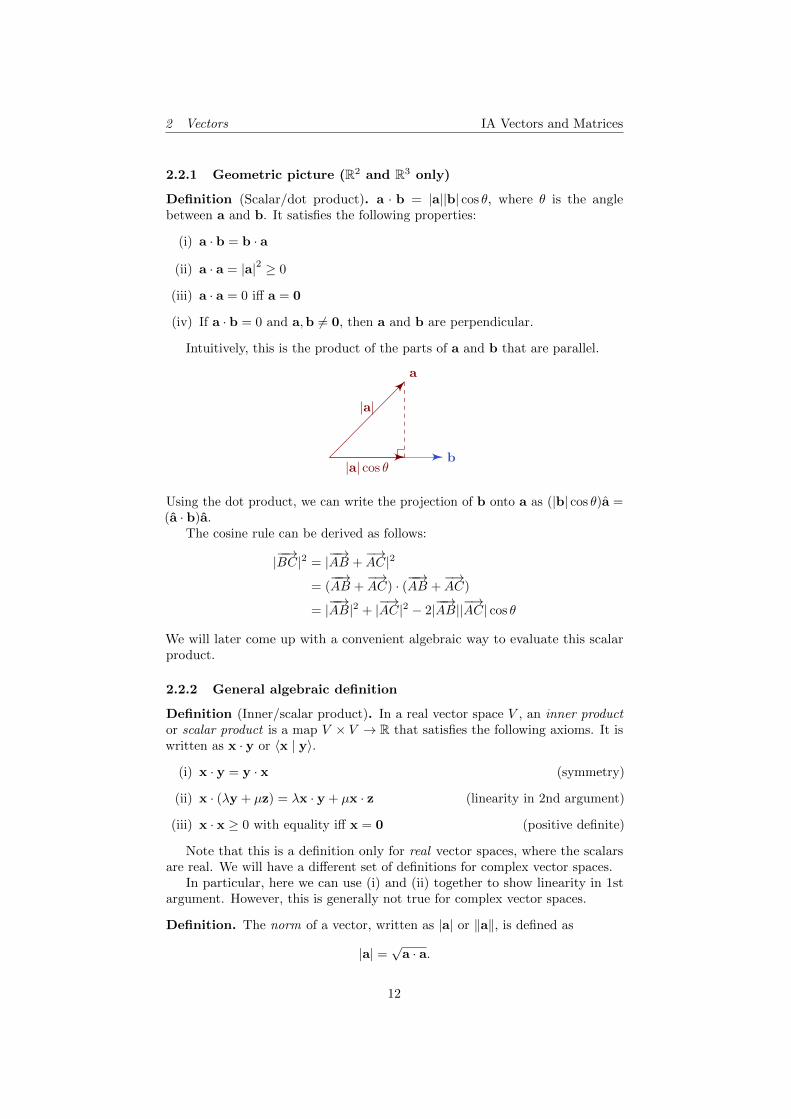
Definition (Scalar/dot product). a · b = |a||b| cos θ, where θ is the anglebetween a and b. It satisfies the following properties:
(i) a · b = b · a
(ii) a · a = |a|2 ≥ 0
(iii) a · a = 0 iff a = 0
(iv) If a · b = 0 and a,b 6= 0, then a and b are perpendicular.
Intuitively, this is the product of the parts of a and b that are parallel.
b
a
|a|
|a| cos θ
Using the dot product, we can write the projection of b onto a as (|b| cos θ)a =(a · b)a.
The cosine rule can be derived as follows:
|−−→BC|2 = |
−−→AB +
−→AC|2
= (−−→AB +
−→AC) · (
−−→AB +
−→AC)
= |−−→AB|2 + |
−→AC|2 − 2|
−−→AB||
−→AC| cos θ
We will later come up with a convenient algebraic way to evaluate this scalarproduct.
2.2.2 General algebraic definition
Definition (Inner/scalar product). In a real vector space V , an inner productor scalar product is a map V × V → R that satisfies the following axioms. It iswritten as x · y or 〈x | y〉.
(i) x · y = y · x (symmetry)
(ii) x · (λy + µz) = λx · y + µx · z (linearity in 2nd argument)
(iii) x · x ≥ 0 with equality iff x = 0 (positive definite)
Note that this is a definition only for real vector spaces, where the scalarsare real. We will have a different set of definitions for complex vector spaces.
In particular, here we can use (i) and (ii) together to show linearity in 1stargument. However, this is generally not true for complex vector spaces.
Definition. The norm of a vector, written as |a| or ‖a‖, is defined as
|a| =√
a · a.
12

2 Vectors IA Vectors and Matrices
Example. Instead of the usual Rn vector space, we can consider the set of allreal (integrable) functions as a vector space. We can define the following innerproduct:
〈f | g〉 =
∫ 1
0
f(x)g(x) dx.
2.3 Cauchy-Schwarz inequality
Theorem (Cauchy-Schwarz inequality). For all x,y ∈ Rn,
|x · y| ≤ |x||y|.
Proof. Consider the expression |x− λy|2. We must have
|x− λy|2 ≥ 0
(x− λy) · (x− λy) ≥ 0
λ2|y|2 − λ(2x · y) + |x|2 ≥ 0.
Viewing this as a quadratic in λ, we see that the quadratic is non-negative andthus cannot have 2 real roots. Thus the discriminant ∆ ≤ 0. So
4(x · y)2 ≤ 4|y|2|x|2
(x · y)2 ≤ |x|2|y|2
|x · y| ≤ |x||y|.
Note that we proved this using the axioms of the scalar product. So thisresult holds for all possible scalar products on any (real) vector space.
Example. Let x = (α, β, γ) and y = (1, 1, 1). Then by the Cauchy-Schwarzinequality, we have
α+ β + γ ≤√
3√α2 + β2 + γ2
α2 + β2 + γ2 ≥ αβ + βγ + γα,
with equality if α = β = γ.
Corollary (Triangle inequality).
|x + y| ≤ |x|+ |y|.
Proof.
|x + y|2 = (x + y) · (x + y)
= |x|2 + 2x · y + |y|2
≤ |x|2 + 2|x||y|+ |y|2
= (|x|+ |y|)2.
So
|x + y| ≤ |x|+ |y|.
13

2 Vectors IA Vectors and Matrices
2.4 Vector product
Apart from the scalar product, we can also define the vector product. However,this is defined only for R3 space, but not spaces in general.
Definition (Vector/cross product). Consider a,b ∈ R3. Define the vectorproduct
a× b = |a||b| sin θn,
where n is a unit vector perpendicular to both a and b. Since there are two(opposite) unit vectors that are perpendicular to both of them, we pick n to bethe one that is perpendicular to a,b in a right-handed sense.
a
b
a× b
The vector product satisfies the following properties:
(i) a× b = −b× a.
(ii) a× a = 0.
(iii) a× b = 0⇒ a = λb for some λ ∈ R (or b = 0).
(iv) a× (λb) = λ(a× b).
(v) a× (b + c) = a× b + a× c.
If we have a triangle OAB, its area is given by 12 |−→OA||
−−→OB| sin θ = 1
2 |−→OA×
−−→OB|.
We define the vector area as 12
−→OA×
−−→OB, which is often a helpful notion when
we want to do calculus with surfaces.There is a convenient way of calculating vector products:
Proposition.
a× b = (a1 i + a2j + a3k)× (b1 i + b2j + b3k)
= (a2b3 − a3b2)i + · · ·
=
∣∣∣∣∣∣i j ka1 a2 a3
b1 b2 b3
∣∣∣∣∣∣2.5 Scalar triple product
Definition (Scalar triple product). The scalar triple product is defined as
[a,b, c] = a · (b× c).
14

2 Vectors IA Vectors and Matrices
Proposition. If a parallelepiped has sides represented by vectors a,b, c thatform a right-handed system, then the volume of the parallelepiped is given by[a,b, c].
b
c
a
Proof. The area of the base of the parallelepiped is given by |b||c| sin θ = |b× c|.Thus the volume= |b× c||a| cosφ = |a · (b× c)|, where φ is the angle betweena and the normal to b and c. However, since a,b, c form a right-handed system,we have a · (b× c) ≥ 0. Therefore the volume is a · (b× c).
Since the order of a,b, c doesn’t affect the volume, we know that
[a,b, c] = [b, c,a] = [c,a,b] = −[b,a, c] = −[a, c,b] = −[c,b,a].
Theorem. a× (b + c) = a× b + a× c.
Proof. Let d = a× (b + c)− a× b− a× c. We have
d · d = d · [a× (b + c)]− d · (a× b)− d · (a× c)
= (b + c) · (d× a)− b · (d× a)− c · (d× a)
= 0
Thus d = 0.
2.6 Spanning sets and bases
2.6.1 2D space
Definition (Spanning set). A set of vectors {a,b} spans R2 if for all vectorsr ∈ R2, there exist some λ, µ ∈ R such that r = λa + µb.
In R2, two vectors span the space if a× b 6= 0.
Theorem. The coefficients λ, µ are unique.
Proof. Suppose that r = λa + µb = λ′a + µ′b. Take the vector product with aon both sides to get (µ− µ′)a× b = 0. Since a× b 6= 0, then µ = µ′. Similarly,λ = λ′.
Definition (Linearly independent vectors in R2). Two vectors a and b arelinearly independent if for α, β ∈ R, αa + βb = 0 iff α = β = 0. In R2, a and bare linearly independent if a× b 6= 0.
Definition (Basis of R2). A set of vectors is a basis of R2 if it spans R2 andare linearly independent.
Example. {i, j} = {(1, 0), (0, 1)} is a basis of R2. They are the standard basisof R2.
15

2 Vectors IA Vectors and Matrices
2.6.2 3D space
We can extend the above definitions of spanning set and linear independent setto R3. Here we have
Theorem. If a,b, c ∈ R3 are non-coplanar, i.e. a · (b× c) 6= 0, then they forma basis of R3.
Proof. For any r, write r = λa + µb + νc. Performing the scalar productwith b× c on both sides, one obtains r · (b× c) = λa · (b× c) + µb · (b× c) +νc · (b× c) = λ[a,b, c]. Thus λ = [r,b, c]/[a,b, c]. The values of µ and ν canbe found similarly. Thus each r can be written as a linear combination of a,band c.
By the formula derived above, it follows that if αa + βb + γc = 0, thenα = β = γ = 0. Thus they are linearly independent.
Note that while we came up with formulas for λ, µ and ν, we did not actuallyprove that these coefficients indeed work. This is rather unsatisfactory. Wecould, of course, expand everything out and show that this indeed works, butin IB Linear Algebra, we will prove a much more general result, saying that ifwe have an n-dimensional space and a set of n linear independent vectors, thenthey form a basis.
In R3, the standard basis is i, j, k, or (1, 0, 0), (0, 1, 0) and (0, 0, 1).
2.6.3 Rn space
In general, we can define
Definition (Linearly independent vectors). A set of vectors {v1,v2,v3 · · ·vm}is linearly independent if
m∑i=1
λivi = 0⇒ (∀i)λi = 0.
Definition (Spanning set). A set of vectors {u1,u2,u3 · · ·um} ⊆ Rn is aspanning set of Rn if
(∀x ∈ Rn)(∃λi)n∑i=1
λiui = x
Definition (Basis vectors). A basis of Rn is a linearly independent spanningset. The standard basis of Rn is e1 = (1, 0, 0, · · · 0), e2 = (0, 1, 0, · · · 0), · · · en =(0, 0, 0, · · · , 1).
Definition (Orthonormal basis). A basis {ei} is orthonormal if ei · ej = 0 ifi 6= j and ei · ei = 1 for all i, j.
Using the Kronecker Delta symbol, which we will define later, we can writethis condition as ei · ej = δij .
Definition (Dimension of vector space). The dimension of a vector space is thenumber of vectors in its basis. (Exercise: show that this is well-defined)
We usually denote the components of a vector x by xi. So we have x =(x1, x2, · · · , xn).
16

2 Vectors IA Vectors and Matrices
Definition (Scalar product). The scalar product of x,y ∈ Rn is defined asx · y =
∑xiyi.
The reader should check that this definition coincides with the |x||y| cos θdefinition in the case of R2 and R3.
2.6.4 Cn space
Cn is very similar to Rn, except that we have complex numbers. As a result, weneed a different definition of the scalar product. If we still defined u ·v =
∑uivi,
then if we let u = (0, i), then u · u = −1 < 0. This would be bad if we want touse the scalar product to define a norm.
Definition (Cn). Cn = {(z1, z2, · · · , zn) : zi ∈ C}. It has the same standardbasis as Rn but the scalar product is defined differently. For u,v ∈ Cn, u · v =∑u∗i vi. The scalar product has the following properties:
(i) u · v = (v · u)∗
(ii) u · (λv + µw) = λ(u · v) + µ(u ·w)
(iii) u · u ≥ 0 and u · u = 0 iff u = 0
Instead of linearity in the first argument, here we have (λu + µv) · w =λ∗u ·w + µ∗v ·w.
Example.
4∑k=1
(−i)k|x + iky|2
=∑
(−i)k〈x + iky | x + iky〉
=∑
(−i)k(〈x + iky | x〉+ ik〈x + iky | y〉)
=∑
(−i)k(〈x | x〉+ (−i)k〈y | x〉+ ik〈x | y〉+ ik(−i)k〈y | y〉)
=∑
(−i)k[(|x|2 + |y|2) + (−1)k〈y | x〉+ 〈x | y〉]
= (|x|2 + |y|2)∑
(−i)k + 〈y | x〉∑
(−1)k + 〈x | y〉∑
1
= 4〈x | y〉.
We can prove the Cauchy-Schwarz inequality for complex vector spaces usingthe same proof as the real case, except that this time we have to first multiply yby some eiθ so that x · (eiθy) is a real number. The factor of eiθ will drop off atthe end when we take the modulus signs.
2.7 Vector subspaces
Definition (Vector subspace). A vector subspace of a vector space V is a subsetof V that is also a vector space under the same operations. Both V and {0} aresubspaces of V . All others are proper subspaces.
A useful criterion is that a subset U ⊆ V is a subspace iff
(i) x,y ∈ U ⇒ (x + y) ∈ U .
17

2 Vectors IA Vectors and Matrices
(ii) x ∈ U ⇒ λx ∈ U for all scalars λ.
(iii) 0 ∈ U .
This can be more concisely written as “U is non-empty and for all x,y ∈ U ,(λx + µy) ∈ U”.
Example.
(i) If {a,b, c} is a basis of R3, then {a + c,b + c} is a basis of a 2D subspace.
Suppose x,y ∈ span{a + c,b + c}. Let
x = α1(a + c) + β1(b + c);
y = α2(a + c) + β2(b + c).
Then
λx+µy = (λα1 +µα2)(a + c) + (λβ1 +µβ2)(b + c) ∈ span{a + c,b + c}.
Thus this is a subspace of R3.
Now check that a + c,b + c is a basis. We only need to check linearindependence. If α(a + c) + β(b + c) = 0, then αa + βb + (α+ β)c = 0.Since {a,b, c} is a basis of R3, therefore a,b, c are linearly independentand α = β = 0. Therefore a + c,b + c is a basis and the subspace hasdimension 2.
(ii) Given a set of numbers αi, let U = {x ∈ Rn :∑ni=1 αixi = 0}. We show
that this is a vector subspace of Rn: Take x,y ∈ U , then consider λx +µy.We have
∑αi(λxi + µyi) = λ
∑αixi + µ
∑αiyi = 0. Thus λx + µy ∈ U .
The dimension of the subspace is n − 1 as we can freely choose xi fori = 1, · · · , n− 1 and then xn is uniquely determined by the previous xi’s.
(iii) Let W = {x ∈ Rn :∑αixi = 1}. Then
∑αi(λxi + µyi) = λ + µ 6= 1.
Therefore W is not a vector subspace.
2.8 Suffix notation
Here we are going to introduce a powerful notation that can help us simplify alot of things.
First of all, let v ∈ R3. We can write v = v1e1 + v2e2 + v3e3 = (v1, v2, v3).So in general, the ith component of v is written as vi. We can thus writevector equations in component form. For example, a = b → ai = bi orc = αa + βb → ci = αai + βbi. A vector has one free suffix, i, while a scalarhas none.
Notation (Einstein’s summation convention). Consider a sum x · y =∑xiyi.
The summation convention says that we can drop the∑
symbol and simplywrite x · y = xiyi. If suffixes are repeated once, summation is understood.
Note that i is a dummy suffix and doesn’t matter what it’s called, i.e.xiyi = xjyj = xkyk etc.
The rules of this convention are:
(i) Suffix appears once in a term: free suffix
18
2 Vectors IA Vectors and Matrices
(ii) Suffix appears twice in a term: dummy suffix and is summed over
(iii) Suffix appears three times or more: WRONG!
Example. [(a · b)c− (a · c)b]i = ajbjci − ajcjbi summing over j understood.
It is possible for an item to have more than one index. These objects areknown as tensors, which will be studied in depth in the IA Vector Calculuscourse.
Here we will define two important tensors:
Definition (Kronecker delta).
δij =
{1 i = j
0 i 6= j.
We have δ11 δ12 δ13
δ21 δ22 δ23
δ31 δ32 δ33
=
1 0 00 1 00 0 1
= I.
So the Kronecker delta represents an identity matrix.
Example.
(i) aiδi1 = a1. In general, aiδij = aj (i is dummy, j is free).
(ii) δijδjk = δik
(iii) δii = n if we are in Rn.
(iv) apδpqbq = apbp with p, q both dummy suffices and summed over.
Definition (Alternating symbol εijk). Consider rearrangements of 1, 2, 3. Wecan divide them into even and odd permutations. Even permutations include(1, 2, 3), (2, 3, 1) and (3, 1, 2). These are permutations obtained by performingtwo (or no) swaps of the elements of (1, 2, 3). (Alternatively, it is any “rotation”of (1, 2, 3))
The odd permutations are (2, 1, 3), (1, 3, 2) and (3, 2, 1). They are thepermutations obtained by one swap only.
Define
εijk =
+1 ijk is even permutation
−1 ijk is odd permutation
0 otherwise (i.e. repeated suffices)
εijk has 3 free suffices.We have ε123 = ε231 = ε312 = +1 and ε213 = ε132 = ε321 = −1. ε112 =
ε111 = · · · = 0.
We have
(i) εijkδjk = εijj = 0
(ii) If ajk = akj (i.e. aij is symmetric), then εijkajk = εijkakj = −εikjakj .Since εijkajk = εikjakj (we simply renamed dummy suffices), we haveεijkajk = 0.
19

2 Vectors IA Vectors and Matrices
Proposition. (a× b)i = εijkajbk
Proof. By expansion of formula
Theorem. εijkεipq = δjpδkq − δjqδkp
Proof. Proof by exhaustion:
RHS =
+1 if j = p and k = q
−1 if j = q and k = p
0 otherwise
LHS: Summing over i, the only non-zero terms are when j, k 6= i and p, q 6= i.If j = p and k = q, LHS is (−1)2 or (+1)2 = 1. If j = q and k = p, LHS is(+1)(−1) or (−1)(+1) = −1. All other possibilities result in 0.
Equally, we have εijkεpqk = δipδjq − δjpδiq and εijkεpjq = δipδkq − δiqδkp.
Proposition.a · (b× c) = b · (c× a)
Proof. In suffix notation, we have
a · (b× c) = ai(b× c)i = εijkbjckai = εjkibjckai = b · (c× a).
Theorem (Vector triple product).
a× (b× c) = (a · c)b− (a · b)c.
Proof.
[a× (b× c)]i = εijkaj(b× c)k= εijkεkpqajbpcq
= εijkεpqkajbpcq
= (δipδjq − δiqδjp)ajbpcq= ajbicj − ajcibj= (a · c)bi − (a · b)ci
Similarly, (a× b)× c = (a · c)b− (b · c)a.
Spherical trigonometry
Proposition. (a× b) · (b× c) = (a · a)(b · c)− (a · b)(a · c).
Proof.
LHS = (a× b)i(a× c)i
= εijkajbkεipqapcq
= (δjpδkq − δjqδkp)ajbkapcq= ajbkajck − ajbkakcj= (a · a)(b · c)− (a · b)(a · c)
20

2 Vectors IA Vectors and Matrices
Consider the unit sphere, center O, with a,b, c on the surface.
A
B C
δ(A,B) α
Suppose we are living on the surface of the sphere. So the distance from A to B isthe arc length on the sphere. We can imagine this to be along the circumferenceof the circle through A and B with center O. So the distance is ∠AOB, which weshall denote by δ(A,B). So a · b = cos∠AOB = cos δ(A,B). We obtain similarexpressions for other dot products. Similarly, we get |a× b| = sin δ(A,B).
cosα =(a× b) · (a× c)
|a× b||a× c|
=b · c− (a · b)(a · c)
|a× b||a× c|
Putting in our expressions for the dot and cross products, we obtain
cosα sin δ(A,B) sin δ(A,C) = cos δ(B,C)− cos δ(A,B) cos δ(A,C).
This is the spherical cosine rule that applies when we live on the surface of asphere. What does this spherical geometry look like?
Consider a spherical equilateral triangle. Using the spherical cosine rule,
cosα =cos δ − cos2 δ
sin2 δ= 1− 1
1 + cos δ.
Since cos δ ≤ 1, we have cosα ≤ 12 and α ≥ 60◦. Equality holds iff δ = 0, i.e. the
triangle is simply a point. So on a sphere, each angle of an equilateral triangle isgreater than 60◦, and the angle sum of a triangle is greater than 180◦.
2.9 Geometry
2.9.1 Lines
Any line through a and parallel to t can be written as
x = a + λt.
By crossing both sides of the equation with t, we have
Theorem. The equation of a straight line through a and parallel to t is
(x− a)× t = 0 or x× t = a× t.
21

2 Vectors IA Vectors and Matrices
2.9.2 Plane
To define a plane Π, we need a normal n to the plane and a fixed point b. Forany x ∈ Π, the vector x− b is contained in the plane and is thus normal to n,i.e. (x− b) · n = 0.
Theorem. The equation of a plane through b with normal n is given by
x · n = b · n.
If n = n is a unit normal, then d = x · n = b · n is the perpendicular distancefrom the origin to Π.
Alternatively, if a,b, c lie in the plane, then the equation of the plane is
(x− a) · [(b− a)× (c− a)] = 0.
Example.
(i) Consider the intersection between a line x× t = a× t with the planex · n = b · n. Cross n on the right with the line equation to obtain
(x · n)t− (t · n)x = (a× t)× n
Eliminate x · n using x · n = b · n
(t · n)x = (b · n)t− (a× t)× n
Provided t · n is non-zero, the point of intersection is
x =(b · n)t− (a× t)× n
t · n.
Exercise: what if t · n = 0?
(ii) Shortest distance between two lines. Let L1 be (x− a1)× t1 = 0 and L2
be (x− a2)× t2 = 0.
The distance of closest approach s is along a line perpendicular to both L1
and L2, i.e. the line of closest approach is perpendicular to both lines andthus parallel to t1 × t2. The distance s can then be found by projecting
a1 − a2 onto t1 × t2. Thus s =∣∣∣(a1 − a2) · t1×t2
|t1×t2|
∣∣∣.2.10 Vector equations
Example. x− (x× a)× b = c. Strategy: take the dot or cross of the equationwith suitable vectors. The equation can be expanded to form
x− (x · b)a + (a · b)x = c.
Dot this with b to obtain
x · b− (x · b)(a · b) + (a · b)(x · b) = c · bx · b = c · b.
22

2 Vectors IA Vectors and Matrices
Substituting this into the original equation, we have
x(1 + a · b) = c + (c · b)a
If (1 + a · b) is non-zero, then
x =c + (c · b)a
1 + a · b
Otherwise, when (1 + a · b) = 0, if c + (c · b)a 6= 0, then a contradiction isreached. Otherwise, x · b = c · b is the most general solution, which is a planeof solutions.
23

3 Linear maps IA Vectors and Matrices
3 Linear maps
A linear map is a special type of function between vector spaces. In fact, mostof the time, these are the only functions we actually care about. They are mapsthat satisfy the property f(λa + µb) = λf(a) + µf(b).
We will first look at two important examples of linear maps — rotations andreflections, and then study their properties formally.
3.1 Examples
3.1.1 Rotation in R3
In R3, first consider the simple cases where we rotate about the z axis by θ. Wecall this rotation R and write x′ = R(x).
Suppose that initially, x = (x, y, z) = (r cosφ, r sinφ, z). Then after arotation by θ, we get
x′ = (r cos(φ+ θ), r sin(φ+ θ), z)
= (r cosφ cos θ − r sinφ sin θ, r sinφ cos θ + r cosφ sin θ, z)
= (x cos θ − y sin θ, x sin θ + y cos θ, z).
We can represent this by a matrix R such that x′i = Rijxj . Using our formulaabove, we obtain
R =
cos θ − sin θ 0sin θ cos θ 0
0 0 1
Now consider the general case where we rotate by θ about n.
O
n
A
x
B
A′
Cx′B A
A′
C
θ
We have x′ =−−→OB +
−−→BC +
−−→CA′. We know that
−−→OB = (n · x)n−−→BC =
−−→BA cos θ
= (−−→BO +
−→OA) cos θ
= (−(n · x)n + x) cos θ
Finally, to get−→CA, we know that |
−−→CA′| = |
−−→BA′| sin θ = |
−−→BA| sin θ = |n× x| sin θ.
Also,−−→CA′ is parallel to n× x. So we must have
−−→CA′ = (n× x) sin θ.
24
3 Linear maps IA Vectors and Matrices
Thus x′ = x cos θ + (1− cos θ)(n · x)n + n× x sin θ. In components,
x′i = xi cos θ + (1− cos θ)njxjni − εijkxjnk sin θ.
We want to find an R such that x′i = Rijxj . So
Rij = δij cos θ + (1− cos θ)ninj − εijknk sin θ.
3.1.2 Reflection in R3
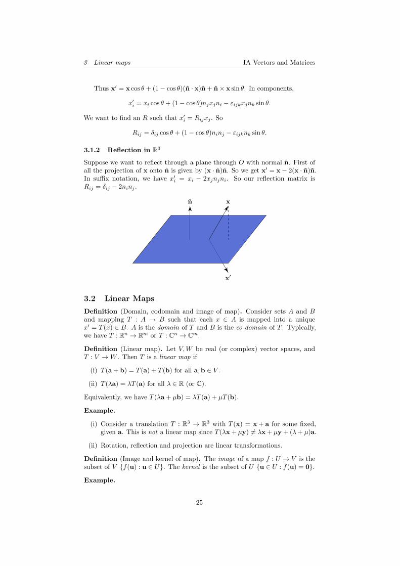
Suppose we want to reflect through a plane through O with normal n. First ofall the projection of x onto n is given by (x · n)n. So we get x′ = x− 2(x · n)n.In suffix notation, we have x′i = xi − 2xjnjni. So our reflection matrix isRij = δij − 2ninj .
x′
n x
3.2 Linear Maps
Definition (Domain, codomain and image of map). Consider sets A and Band mapping T : A → B such that each x ∈ A is mapped into a uniquex′ = T (x) ∈ B. A is the domain of T and B is the co-domain of T . Typically,we have T : Rn → Rm or T : Cn → Cm.
Definition (Linear map). Let V,W be real (or complex) vector spaces, andT : V →W . Then T is a linear map if
(i) T (a + b) = T (a) + T (b) for all a,b ∈ V .
(ii) T (λa) = λT (a) for all λ ∈ R (or C).
Equivalently, we have T (λa + µb) = λT (a) + µT (b).
Example.
(i) Consider a translation T : R3 → R3 with T (x) = x + a for some fixed,given a. This is not a linear map since T (λx + µy) 6= λx + µy + (λ+ µ)a.
(ii) Rotation, reflection and projection are linear transformations.
Definition (Image and kernel of map). The image of a map f : U → V is thesubset of V {f(u) : u ∈ U}. The kernel is the subset of U {u ∈ U : f(u) = 0}.
Example.
25
3 Linear maps IA Vectors and Matrices
(i) Consider S : R3 → R2 with S(x, y, z) = (x + y, 2x − z). Simple yettedious algebra shows that this is linear. Now consider the effect of S onthe standard basis. S(1, 0, 0) = (1, 2), S(0, 1, 0) = (1, 0) and S(0, 0, 1) =(0,−1). Clearly these are linearly dependent, but they do span the wholeof R2. We can say S(R3) = R2. So the image is R2.
Now solve S(x, y, z) = 0. We need x+ y = 0 and 2x− z = 0. Thus x =(x,−x, 2x), i.e. it is parallel to (1,−1, 2). So the set {λ(1,−1, 2) : λ ∈ R}is the kernel of S.
(ii) Consider a rotation in R3. The kernel is the zero vector and the image isR3.
(iii) Consider a projection of x onto a plane with normal n. The image is theplane itself, and the kernel is any vector parallel to n
Theorem. Consider a linear map f : U → V , where U, V are vector spaces.Then im(f) is a subspace of V , and ker(f) is a subspace of U .
Proof. Both are non-empty since f(0) = 0.If x,y ∈ im(f), then ∃a,b ∈ U such that x = f(a),y = f(b). Then
λx + µy = λf(a) + µf(b) = f(λa + µb). Now λa + µb ∈ U since U is a vectorspace, so there is an element in U that maps to λx + µy. So λx + µy ∈ im(f)and im(f) is a subspace of V .
Suppose x,y ∈ ker(f), i.e. f(x) = f(y) = 0. Then f(λx + µy) = λf(x) +µf(y) = λ0 + µ0 = 0. Therefore λx + µy ∈ ker(f).
3.3 Rank and nullity
Definition (Rank of linear map). The rank of a linear map f : U → V , denotedby r(f), is the dimension of the image of f .
Definition (Nullity of linear map). The nullity of f , denoted n(f) is thedimension of the kernel of f .
Example. For the projection onto a plane in R3, the image is the whole planeand the rank is 2. The kernel is a line so the nullity is 1.
Theorem (Rank-nullity theorem). For a linear map f : U → V ,
r(f) + n(f) = dim(U).
Proof. (Non-examinable) Write dim(U) = n and n(f) = m. If m = n, then f isthe zero map, and the proof is trivial, since r(f) = 0. Otherwise, assume m < n.
Suppose {e1, e2, · · · , em} is a basis of ker f , Extend this to a basis of thewhole of U to get {e1, e2, · · · , em, em+1, · · · , en}. To prove the theorem, weneed to prove that {f(em+1), f(em+2), · · · f(en)} is a basis of im(f).
(i) First show that it spans im(f). Take y ∈ im(f). Thus ∃x ∈ U such thaty = f(x). Then
y = f(α1e1 + α2e2 + · · ·+ αnen),
since e1, · · · en is a basis of U . Thus
y = α1f(e1) +α2f(e2) + · · ·+αmf(em) +αm+1f(em+1) + · · ·+αnf(en).
26

3 Linear maps IA Vectors and Matrices
The first m terms map to 0, since e1, · · · em is the basis of the kernel of f .Thus
y = αm+1f(em+1) + · · ·+ αnf(en).
(ii) To show that they are linearly independent, suppose
αm+1f(em+1) + · · ·+ αnf(en) = 0.
Thenf(αm+1em+1 + · · ·+ αnen) = 0.
Thus αm+1em+1 + · · ·+ αnen ∈ ker(f). Since {e1, · · · , em} span ker(f),there exist some α1, α2, · · ·αm such that
αm+1em+1 + · · ·+ αnen = α1e1 + · · ·+ αmem.
But e1 · · · en is a basis of U and are linearly independent. So αi = 0 for all i.Then the only solution to the equation αm+1f(em+1) + · · ·+ αnf(en) = 0is αi = 0, and they are linearly independent by definition.
Example. Calculate the kernel and image of f : R3 → R3, defined by f(x, y, z) =(x+ y + z, 2x− y + 5z, x+ 2z).
First find the kernel: we’ve got the system of equations:
x+ y + z = 0
2x− y + 5z = 0
x+ 2z = 0
Note that the first and second equation add to give 3x+6z = 0, which is identicalto the third. Then using the first and third equation, we have y = −x− z = z.So the kernel is any vector in the form (−2z, z, z) and is the span of (−2, 1, 1).
To find the image, extend the basis of ker(f) to a basis of the whole of R3:{(−2, 1, 1), (0, 1, 0), (0, 0, 1)}. Apply f to this basis to obtain (0, 0, 0), (1,−1, 0)and (1, 5, 2). From the proof of the rank-nullity theorem, we know that f(0, 0, 1)and f(0, 0, 1) is a basis of the image.
To get the standard form of the image, we know that the normal to the planeis parallel to (1,−1, 0)× (1, 5, 2) ‖ (1, 1,−3). Since 0 ∈ im(f), the equation ofthe plane is x+ y − 3z = 0.
3.4 Matrices
In the examples above, we have represented our linear maps by some object Rsuch that x′i = Rijxj . We call R the matrix for the linear map. In general, letα : Rn → Rm be a linear map, and x′ = α(x).
Let {ei} be a basis of Rn. Then x = xjej for some xj . Then we get
x′ = α(xjej) = xjα(ej).
So we get thatx′i = [α(ej)]ixj .
27
3 Linear maps IA Vectors and Matrices
We now define Aij = [α(ej)]i. Then x′i = Aijxj . We write
A = {Aij} =
A11 · · · A1n
... Aij...
Am1 · · · Amn
Here Aij is the entry in the ith row of the jth column. We say that A is anm× n matrix, and write x′ = Ax.
We see that the columns of the matrix are the images of the standard basisvectors under the mapping α.
Example.
3.4.1 Examples
(i) In R2, consider a reflection in a line with an angle θ to the x axis. Weknow that i 7→ cos 2θi + sin 2θj , with j 7→ − cos 2θj + sin 2θi. Then the
matrix is
(cos 2θ sin 2θsin 2θ − cos 2θ
).
(ii) In R3, as we’ve previously seen, a rotation by θ about the z axis is givenby
R =
cos θ − sin θ 0sin θ cos θ 0
0 0 1
(iii) In R3, a reflection in plane with normal n is given by Rij = δij − 2ninj .
Written as a matrix, we have1− 2n21 −2n1n2 −2n1n3
−2n2n1 1− 2n22 −2n2n3
−2n3n1 −2n3n2 1− 2n23
(iv) Dilation (“stretching”) α : R3 → R3 is given by a map (x, y, z) 7→
(λx, µy, νz) for some λ, µ, ν. The matrix isλ 0 00 µ 00 0 ν
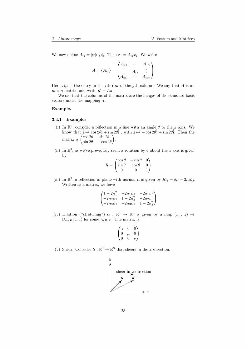
(v) Shear: Consider S : R3 → R3 that sheers in the x direction:
x
y
x x′sheer in x direction
28

3 Linear maps IA Vectors and Matrices
We have (x, y, z) 7→ (x+ λy, y, z). Then
S =
1 λ 00 1 00 0 1
3.4.2 Matrix Algebra
This part is mostly on a whole lot of definitions, saying what we can do withmatrices and classifying them into different types.
Definition (Addition of matrices). Consider two linear maps α, β : Rn → Rm.The sum of α and β is defined by
(α+ β)(x) = α(x) + β(x)
In terms of the matrix, we have
(A+B)ijxj = Aijxj +Bijxj ,
or
(A+B)ij = Aij +Bij .
Definition (Scalar multiplication of matrices). Define (λα)x = λ[α(x)]. So(λA)ij = λAij .
Definition (Matrix multiplication). Consider maps α : R` → Rn and β :Rn → Rm. The composition is βα : R` → Rm. Take x ∈ R` 7→ x′′ ∈ Rm.Then x′′ = (BA)x = Bx′, where x′ = Ax. Using suffix notation, we havex′′i = (Bx′)i = bikx
′k = BikAkjxj . But x′′i = (BA)ijxj . So
(BA)ij = BikAkj .
Generally, an m× n matrix multiplied by an n× ` matrix gives an m× ` matrix.(BA)ij is given by the ith row of B dotted with the jth column of A.
Note that the number of columns of B has to be equal to the number of rowsof A for multiplication to be defined. If ` = m as well, then both BA and ABmake sense, but AB 6= BA in general. In fact, they don’t even have to have thesame dimensions.
Also, since function composition is associative, we get A(BC) = (AB)C.
Definition (Transpose of matrix). If A is an m× n matrix, the transpose AT
is an n×m matrix defined by (AT )ij = Aji.
Proposition.
(i) (AT )T = A.
(ii) If x is a column vector
x1
x2
...xn
, xT is a row vector (x1 x2 · · ·xn).
29

3 Linear maps IA Vectors and Matrices
(iii) (AB)T = BTAT since (AB)Tij = (AB)ji = AjkBki = BkiAjk= (BT )ik(AT )kj = (BTAT )ij .
Definition (Hermitian conjugate). Define A† = (AT )∗. Similarly, (AB)† =B†A†.
Definition (Symmetric matrix). A matrix is symmetric if AT = A.
Definition (Hermitian matrix). A matrix is Hermitian if A† = A. (The diagonalof a Hermitian matrix must be real).
Definition (Anti/skew symmetric matrix). A matrix is anti-symmetric or skewsymmetric if AT = −A. The diagonals are all zero.
Definition (Skew-Hermitian matrix). A matrix is skew-Hermitian if A† = −A.The diagonals are pure imaginary.
Definition (Trace of matrix). The trace of an n× n matrix A is the sum of thediagonal. tr(A) = Aii.
Example. Consider the reflection matrix Rij = δij − 2ninj . We have tr(A) =Rii = 3− 2n · n = 3− 2 = 1.
Proposition. tr(BC) = tr(CB)
Proof. tr(BC) = BikCki = CkiBik = (CB)kk = tr(CB)
Definition (Identity matrix). I = δij .
3.4.3 Decomposition of an n× n matrix
Any n×n matrix B can be split as a sum of symmetric and antisymmetric parts.Write
Bij =1
2(Bij +Bji)︸ ︷︷ ︸
Sij
+1
2(Bij −Bji)︸ ︷︷ ︸
Aij
.
We have Sij = Sji, so S is symmetric, while Aji = −Aij , and A is antisymmetric.So B = S +A.
Furthermore , we can decompose S into an isotropic part (a scalar multipleof the identity) plus a trace-less part (i.e. sum of diagonal = 0). Write
Sij =1
ntr(S)δij︸ ︷︷ ︸
isotropic part
+ (Sij −1
ntr(S)δij)︸ ︷︷ ︸
Tij
.
We have tr(T ) = Tii = Sii − 1n tr(S)δii = tr(S)− 1
n tr(S)(n) = 0.Putting all these together,
B =1
ntr(B)I +
{1
2(B +BT )− 1
ntr(B)I
}+
1
2(B −BT ).
In three dimensions, we can write the antisymmetric part A in terms of a singlevector: we have
A =
0 a −b−a 0 cb −c 0
30

3 Linear maps IA Vectors and Matrices
and we can consider
εijkωk =
0 ω3 −ω2
−ω3 0 ω1
ω2 −ω1 0
So if we have ω = (c, b, a), then Aij = εijkωk.
This decomposition can be useful in certain physical applications. Forexample, if the matrix represents the stress of a system, different parts of thedecomposition will correspond to different types of stresses.
3.4.4 Matrix inverse
Definition (Inverse of matrix). Consider an m×n matrix A and n×m matricesB and C. If BA = I, then we say B is the left inverse of A. If AC = I, thenwe say C is the right inverse of A. If A is square (n× n), then B = B(AC) =(BA)C = C, i.e. the left and right inverses coincide. Both are denoted by A−1,the inverse of A. Therefore we have
AA−1 = A−1A = I.
Note that not all square matrices have inverses. For example, the zero matrixclearly has no inverse.
Definition (Invertible matrix). If A has an inverse, then A is invertible.
Proposition. (AB)−1 = B−1A−1
Proof. (B−1A−1)(AB) = B−1(A−1A)B = B−1B = I.
Definition (Orthogonal and unitary matrices). A real n×n matrix is orthogonalif ATA = AAT = I, i.e. AT = A−1. A complex n × n matrix is unitary ifU†U = UU† = I, i.e. U† = U−1.
Note that an orthogonal matrix A satisfies Aik(ATkj) = δij , i.e. AikAjk = δij .We can see this as saying “the scalar product of two distinct rows is 0, and thescalar product of a row with itself is 1”. Alternatively, the rows (and columns —by considering AT ) of an orthogonal matrix form an orthonormal set.
Similarly, for a unitary matrix, UikU†kj = δij , i.e. uiku
∗jk = u∗ikujk = δij . i.e.
the rows are orthonormal, using the definition of complex scalar product.
Example.
(i) The reflection in a plane is an orthogonal matrix. Since Rij = δij − 2ninj ,We have
RikRjk = (δik − 2nink)(δjk − 2njnk)
= δikδjk − 2δjknink − 2δiknjnk + 2ninknjnk
= δij − 2ninj − 2njni + 4ninj(nknk)
= δij
31

3 Linear maps IA Vectors and Matrices
(ii) The rotation is an orthogonal matrix. We could multiply out using suffixnotation, but it would be cumbersome to do so. Alternatively, denoterotation matrix by θ about n as R(θ, n). Clearly, R(θ, n)−1 = R(−θ, n).We have
Rij(−θ, n) = (cos θ)δij + ninj(1− cos θ) + εijknk sin θ
= (cos θ)δji + njni(1− cos θ)− εjiknk sin θ
= Rji(θ, n)
In other words, R(−θ, n) = R(θ, n)T . So R(θ, n)−1 = R(θ, n)T .
3.5 Determinants
Consider a linear map α : R3 → R3. The standard basis e1, e2, e3 is mapped toe′1, e
′2, e′3 with e′i = Aei. Thus the unit cube formed by e1, e2, e3 is mapped to
the parallelepiped with volume
[e′1, e′2, e′3] = εijk(e′1)i(e
′2)j(e
′3)k
= εijkAi` (e1)`︸ ︷︷ ︸δ1`
Ajm (e2)m︸ ︷︷ ︸δ2m
Akn (e3)n︸ ︷︷ ︸δ3n
= εijkAi1Aj2Ak3
We call this the determinant and write as
det(A) =
∣∣∣∣∣∣A11 A12 A13
A21 A22 A23
A31 A32 A33
∣∣∣∣∣∣3.5.1 Permutations
To define the determinant for square matrices of arbitrary size, we first have toconsider permutations.
Definition (Permutation). A permutation of a set S is a bijection ε : S → S.
Notation. Consider the set Sn of all permutations of 1, 2, 3, · · · , n. Sn containsn! elements. Consider ρ ∈ Sn with i 7→ ρ(i). We write
ρ =
(1 2 · · · nρ(1) ρ(2) · · · ρ(n)
).
Definition (Fixed point). A fixed point of ρ is a k such that ρ(k) = k. e.g. in(1 2 3 44 1 3 2
), 3 is the fixed point. By convention, we can omit the fixed point
and write as
(1 2 44 1 2
).
Definition (Disjoint permutation). Two permutations are disjoint if numbers
moved by one are fixed by the other, and vice versa. e.g.
(1 2 4 5 65 6 1 4 2
)=(
2 66 2
)(1 4 55 1 4
), and the two cycles on the right hand side are disjoint.
Disjoint permutations commute, but in general non-disjoint permutations donot.
32
3 Linear maps IA Vectors and Matrices
Definition (Transposition and k-cycle).
(2 66 2
)is a 2-cycle or a transposition,
and we can simply write (2 6).
(1 4 55 1 4
)is a 3-cycle, and we can simply write
(1 5 4). (1 is mapped to 5; 5 is mapped to 4; 4 is mapped to 1)
Proposition. Any q-cycle can be written as a product of 2-cycles.
Proof. (1 2 3 · · · n) = (1 2)(2 3)(3 4) · · · (n− 1 n).
Definition (Sign of permutation). The sign of a permutation ε(ρ) is (−1)r,where r is the number of 2-cycles when ρ is written as a product of 2-cycles. Ifε(ρ) = +1, it is an even permutation. Otherwise, it is an odd permutation. Notethat ε(ρσ) = ε(ρ)ε(σ) and ε(ρ−1) = ε(ρ).
The proof that this is well-defined can be found in IA Groups.
Definition (Levi-Civita symbol). The Levi-Civita symbol is defined by
εj1j2···jn =
+1 if j1j2j3 · · · jn is an even permutation of 1, 2, · · ·n−1 if it is an odd permutation
0 if any 2 of them are equal
Clearly, ερ(1)ρ(2)···ρ(n) = ε(ρ).
Definition (Determinant). The determinant of an n×n matrix A is defined as:
det(A) =∑σ∈Sn
ε(σ)Aσ(1)1Aσ(2)2 · · ·Aσ(n)n,
or equivalently,det(A) = εj1j2···jnAj11Aj22 · · ·Ajnn.
Proposition. ∣∣∣∣a bc d
∣∣∣∣ = ad− bc
3.5.2 Properties of determinants
Proposition. det(A) = det(AT ).
Proof. Take a single term Aσ(1)1Aσ(2)2 · · ·Aσ(n)n and let ρ be another permuta-tion in Sn. We have
Aσ(1)1Aσ(2)2 · · ·Aσ(n)n = Aσ(ρ(1))ρ(1)Aσ(ρ(2))ρ(2) · · ·Aσ(ρ(n))ρ(n)
since the right hand side is just re-ordering the order of multiplication. Chooseρ = σ−1 and note that ε(σ) = ε(ρ). Then
det(A) =∑ρ∈Sn
ε(ρ)A1σ(1)A2σ(2) · · ·Anσ(n) = det(AT ).
Proposition. If matrix B is formed by multiplying every element in a single rowof A by a scalar λ, then det(B) = λ det(A). Consequently, det(λA) = λn det(A).
33

3 Linear maps IA Vectors and Matrices
Proof. Each term in the sum is multiplied by λ, so the whole sum is multipliedby λn.
Proposition. If 2 rows (or 2 columns) of A are identical, the determinant is 0.
Proof. wlog, suppose columns 1 and 2 are the same. Then
det(A) =∑σ∈Sn
ε(σ)Aσ(1)1Aσ(2)2 · · ·Aσ(n)n.
Now write an arbitrary σ in the form σ = ρ(1 2). Then ε(σ) = ε(ρ)ε((1 2)) =−ε(ρ). So
det(A) =∑ρ∈Sn
−ε(ρ)Aρ(2)1Aρ(1)2Aρ(3)3 · · ·Aρ(n)n.
But columns 1 and 2 are identical, so Aρ(2)1 = Aρ(2)2 and Aρ(1)2 = Aρ(1)1. Sodet(A) = −det(A) and det(A) = 0.
Proposition. If 2 rows or 2 columns of a matrix are linearly dependent, thenthe determinant is zero.
Proof. Suppose in A, (column r) + λ(column s) = 0. Define
Bij =
{Aij j 6= r
Aij + λAis j = r.
Then det(B) = det(A) + λ det(matrix with column r = column s) = det(A).Then we can see that the rth column of B is all zeroes. So each term in the sumcontains one zero and det(A) = det(B) = 0.
Even if we don’t have linearly dependent rows or columns, we can still runthe exact same proof as above, and still get that det(B) = det(A). Lineardependence is only required to show that det(B) = 0. So in general, we can adda linear multiple of a column (or row) onto another column (or row) withoutchanging the determinant.
Proposition. Given a matrix A, if B is a matrix obtained by adding a multipleof a column (or row) of A to another column (or row) of A, then detA = detB.
Corollary. Swapping two rows or columns of a matrix negates the determinant.
Proof. We do the column case only. Let A = (a1 · · ·ai · · ·aj · · ·an). Then
det(a1 · · ·ai · · ·aj · · ·an) = det(a1 · · ·ai + aj · · ·aj · · ·an)
= det(a1 · · ·ai + aj · · ·aj − (ai + aj) · · ·an)
= det(a1 · · ·ai + aj · · · − ai · · ·an)
= det(a1 · · ·aj · · · − ai · · ·an)
= −det(a1 · · ·aj · · ·ai · · ·an)
Alternatively, we can prove this from the definition directly, using the fact thatthe sign of a transposition is −1 (and that the sign is multiplicative).
Proposition. det(AB) = det(A) det(B).
34

3 Linear maps IA Vectors and Matrices
Proof. First note that∑σ ε(σ)Aσ(1)ρ(1)Aσ(2)ρ(2) = ε(ρ) det(A), i.e. swapping
columns (or rows) an even/odd number of times gives a factor ±1 respectively.We can prove this by writing σ = µρ.
Now
detAB =∑σ
ε(σ)(AB)σ(1)1(AB)σ(2)2 · · · (AB)σ(n)n
=∑σ
ε(σ)
n∑k1,k2,··· ,kn
Aσ(1)k1Bk11 · · ·Aσ(n)knBknn
=∑
k1,··· ,kn
Bk11 · · ·Bknn∑σ
ε(σ)Aσ(1)k1Aσ(2)k2 · · ·Aσ(n)kn︸ ︷︷ ︸S
Now consider the many different S’s. If in S, two of k1 and kn are equal, then Sis a determinant of a matrix with two columns the same, i.e. S = 0. So we onlyhave to consider the sum over distinct kis. Thus the kis are are a permutationof 1, · · ·n, say ki = ρ(i). Then we can write
detAB =∑ρ
Bρ(1)1 · · ·Bρ(n)n
∑σ
ε(σ)Aσ(1)ρ(1) · · ·Aσ(n)ρ(n)
=∑ρ
Bρ(1)1 · · ·Bρ(n)n(ε(ρ) detA)
= detA∑ρ
ε(ρ)Bρ(1)1 · · ·Bρ(n)n
= detA detB
Corollary. If A is orthogonal, detA = ±1.
Proof.
AAT = I
detAAT = det I
detA detAT = 1
(detA)2 = 1
detA = ±1
Corollary. If U is unitary, |detU | = 1.
Proof. We have detU† = (detUT )∗ = det(U)∗. Since UU† = I, we havedet(U) det(U)∗ = 1.
Proposition. In R3, orthogonal matrices represent either a rotation (det = 1)or a reflection (det = −1).
3.5.3 Minors and Cofactors
Definition (Minor and cofactor). For an n× n matrix A, define Aij to be the(n− 1)× (n− 1) matrix in which row i and column j of A have been removed.
The minor of the ijth element of A is Mij = detAij
The cofactor of the ijth element of A is ∆ij = (−1)i+jMij .
35

3 Linear maps IA Vectors and Matrices
Notation. We use ¯ to denote a symbol which has been missed out of a naturalsequence.
Example. 1, 2, 3, 5 = 1, 2, 3, 4, 5.
The significance of these definitions is that we can use them to provide asystematic way of evaluating determinants. We will also use them to find inversesof matrices.
Theorem (Laplace expansion formula). For any particular fixed i,
detA =
n∑j=1
Aji∆ji.
Proof.
detA =
n∑ji=1
Ajii
n∑j1,··· ,ji,···jn
εj1j2···jnAj11Aj22 · · ·Ajii · · ·Ajnn
Let σ ∈ Sn be the permutation which moves ji to the ith position, and leaveeverything else in its natural order, i.e.
σ =
(1 · · · i i+ 1 i+ 2 · · · ji − 1 ji ji + 1 · · · n1 · · · ji i i+ 1 · · · ji − 2 ji − 1 ji + 1 · · · n
)if ji > i, and similarly for other cases. To perform this permutation, |i − ji|transpositions are made. So ε(σ) = (−1)i−ji .
Now consider the permutation ρ ∈ Sn
ρ =
(1 · · · · · · ji · · · nj1 · · · ji · · · · · · jn
)The composition ρσ reorders (1, · · · , n) to (j1, j2, · · · , jn). So ε(ρσ) = εj1···jn =ε(ρ)ε(σ) = (−1)i−jiεj1···ji···jn . Hence the original equation becomes
detA =
n∑ji=1
Ajii∑
j1···ji···jn
(−1)i−jiεj1···ji···jnAj11 · · ·Ajii · · ·Ajnn
=
n∑ji=1
Ajii(−1)i−jiMjii
=
n∑ji=1
Ajii∆jii
=
n∑j=1
Aji∆ji
Example. detA =
∣∣∣∣∣∣2 4 23 2 12 0 1
∣∣∣∣∣∣. We can pick the first row and have
detA = 2
∣∣∣∣2 10 1
∣∣∣∣− 4
∣∣∣∣3 12 1
∣∣∣∣+ 2
∣∣∣∣3 22 0
∣∣∣∣= 2(2− 0)− 4(3− 2) + 2(0− 4)
= −8.
36

3 Linear maps IA Vectors and Matrices
Alternatively, we can pick the second column and have
detA = −4
∣∣∣∣3 12 1
∣∣∣∣+ 2
∣∣∣∣2 22 1
∣∣∣∣− 0
∣∣∣∣2 23 1
∣∣∣∣= −4(3− 2) + 2(2− 4)− 0
= −8.
In practical terms, we use a combination of properties of determinants witha sensible choice of i to evaluate det(A).
Example. Consider
∣∣∣∣∣∣1 a a2
1 b b2
1 c c2
∣∣∣∣∣∣. Row 1 - row 2 gives
∣∣∣∣∣∣0 a− b a2 − b21 b b2
1 c c2
∣∣∣∣∣∣ = (a− b)
∣∣∣∣∣∣0 1 a+ b1 b b2
1 c c2
∣∣∣∣∣∣ .Do row 2 - row 3. We obtain
(a− b)(b− c)
∣∣∣∣∣∣0 1 a+ b0 1 b+ c1 c c2
∣∣∣∣∣∣ .Row 1 - row 2 gives
(a− b)(b− c)(a− c)
∣∣∣∣∣∣0 0 10 1 b+ c1 c c2
∣∣∣∣∣∣ = (a− b)(b− c)(a− c).
37
4 Matrices and linear equations IA Vectors and Matrices
4 Matrices and linear equations
4.1 Simple example, 2× 2
Consider the system of equations
A11x1 +A12x2 = d1 (a)
A21x1 +A22x2 = d2. (b)
We can write this as
Ax = d.
If we do (a)×A22−(b)×A12 and similarly the other way round, we obtain
(A11A22 −A12A21)x1 = A22d1 −A12d2
(A11A22 −A12A21)︸ ︷︷ ︸detA
x2 = A11d2 −A21d1
Dividing by detA and writing in matrix form, we have(x1
x2
)=
1
detA
(A22 −A12
−A21 A11
)(d1
d2
)On the other hand, given the equation Ax = d, if A−1 exists, then by multiplyingboth sides on the left by A−1, we obtain x = A−1d.
Hence, we have constructed A−1 in the 2 × 2 case, and shown that thecondition for its existence is detA 6= 0, with
A−1 =1
detA
(A22 −A12
−A21 A11
)
4.2 Inverse of an n× n matrix
For larger matrices, the formula for the inverse is similar, but slightly morecomplicated (and costly to evaluate). The key to finding the inverse is thefollowing:
Lemma.∑Aik∆jk = δij detA.
Proof. If i 6= j, then consider an n× n matrix B, which is identical to A exceptthe jth row is replaced by the ith row of A. So ∆jk of B = ∆jk of A, since ∆jk
does not depend on the elements in row j. Since B has a duplicate row, we knowthat
0 = detB =
n∑k=1
Bjk∆jk =
n∑k=1
Aik∆jk.
If i = j, then the expression is detA by the Laplace expansion formula.
Theorem. If detA 6= 0, then A−1 exists and is given by
(A−1)ij =∆ji
detA.
38

4 Matrices and linear equations IA Vectors and Matrices
Proof.
(A−1)ikAkj =∆ki
detAAkj =
δij detA
detA= δij .
So A−1A = I.
The other direction is easy to prove. If detA = 0, then it has no inverse,since for any matrix B, detAB = 0, and hence AB cannot be the identity.
Example. Consider the shear matrix Sλ =
1 λ 00 1 00 0 1
. We have detSλ = 1.
The cofactors are
∆11 = 1 ∆12 = 0 ∆13 = 0∆21 − λ ∆22 = 1 ∆23 = 0∆31 = 0 ∆32 = 0 ∆33 = 1
So S−1λ =
1 −λ 00 1 00 0 1
.
How many arithmetic operations are involved in calculating the inverse of ann× n matrix? We just count multiplication operations since they are the mosttime-consuming. Suppose that calculating detA takes fn multiplications. Thisinvolves n (n−1)× (n−1) determinants, and you need n more multiplications toput them together. So fn = nfn−1 + n. So fn = O(n!) (in fact fn ≈ (1 + e)n!).
To find the inverse, we need to calculate n2 cofactors. Each is a n − 1determinant, and each takesO((n−1)!). So the time complexity isO(n2(n−1)!) =O(n · n!).
This is incredibly slow. Hence while it is theoretically possible to solvesystems of linear equations by inverting a matrix, sane people do not do soin general. Instead, we develop certain better methods to solve the equations.In fact, the “usual” method people use to solve equations by hand only hascomplexity O(n3), which is a much better complexity.
4.3 Homogeneous and inhomogeneous equations
Consider Ax = b where A is an n× n matrix, x and b are n× 1 column vectors.
Definition (Homogeneous equation). If b = 0, then the system is homogeneous.Otherwise, it’s inhomogeneous.
Suppose detA 6= 0. Then there is a unique solution x = A−1b (x = 0 forhomogeneous).
How can we understand this result? Recall that detA 6= 0 means that thecolumns of A are linearly independent. The columns are the images of the stan-dard basis, e′i = Aei. So detA 6= 0 means that e′i are linearly independent andform a basis of Rn. Therefore the image is the whole of Rn. This automaticallyensures that b is in the image, i.e. there is a solution.
To show that there is exactly one solution, suppose x and x′ are both solutions.Then Ax = Ax′ = b. So A(x − x′) = 0. So x − x′ is in the kernel of A. Butsince the rank of A is n, by the rank-nullity theorem, the nullity is 0. So thekernel is trivial. So x− x′ = 0, i.e. x = x′.
39

4 Matrices and linear equations IA Vectors and Matrices
4.3.1 Gaussian elimination
Consider a general solution
A11x1 +A12x2 + · · ·+A1nxn = d1
A21x1 +A22x2 + · · ·+A2nxn = d2
...
Am1x1 +Am2x2 + · · ·+Amnxn = dm
So we have m equations and n unknowns.Assume A11 6= 0 (if not, we can re-order the equations). We can use the
first equation to eliminate x1 from the remaining (m− 1) equations. Then usethe second equation to eliminate x2 from the remaining (m− 2) equations (ifanything goes wrong, just re-order until things work). Repeat.
We are left with
A11x1 +A12x2 +A13x3 + · · ·+A1nxn = d1
A(2)22 x2 +A
(2)23 x3 + · · ·+A
(2)2n xn = d2
...
A(r)rr xr + · · ·+A(r)
rn xn = dr
0 = d(r)r+1
...
0 = d(r)m
Here A(i)ii 6= 0 (which we can achieve by re-ordering), and the superfix (i) refers
to the “version number” of the coefficient, e.g. A(2)22 is the second version of the
coefficient of x2 in the second row.Let’s consider the different possibilities:
(i) r < m and at least one of d(r)r+1, · · · d
(r)m 6= 0. Then a contradiction is
reached. The system is inconsistent and has no solution. We say it isoverdetermined.
Example. Consider the system
3x1 + 2x2 + x3 = 3
6x1 + 3x2 + 3x3 = 0
6x1 + 2x2 + 4x3 = 6
This becomes
3x1 + 2x2 + x3 = 3
0− x2 + x3 = −6
0− 2x2 + 2x3 = 0
40

4 Matrices and linear equations IA Vectors and Matrices
And then
3x1 + 2x2 + x3 = 3
0− x2 + x3 = −6
0 = 12
We have d(3)3 = 12 = 0 and there is no solution.
(ii) If r = n ≤ m, and all d(r)r+i = 0. Then from the nth equation, there
is a unique solution for xn = d(n)n /A
(n)nn , and hence for all xi by back
substitution. This system is determined.
Example.
2x1 + 5x2 = 2
4x1 + 3x2 = 11
This becomes
2x1 + 5x2 = 2
−7x2 = 7
So x2 = −1 and thus x1 = 7/2.
(iii) If r < n and d(r)r+i = 0, then xr+1, · · ·xn can be freely chosen, and there
are infinitely many solutions. System is under-determined. e.g.
x1 + x2 = 1
2x1 + 2x2 = 2
Which gives
x1 + x2 = 1
0 = 0
So x1 = 1− x2 is a solution for any x2.
In the n = m case, there are O(n3) operations involved, which is much less thaninverting the matrix. So this is an efficient way of solving equations.
This is also be related to the determinant. Consider the case where m = nand A is square. Since row operations do not change the determinant andswapping rows give a factor of (−1). So
detA = (−1)k
∣∣∣∣∣∣∣∣∣∣∣∣∣∣∣
A11 A12 · · · · · · · · · A1n
0 A(2)22 · · · · · · · · · A
(n)2n
......
. . ....
......
0 0 · · · A(r)rr · · · A
(n)rn
0 0 · · · 0 0 · · ·...
......
......
...
∣∣∣∣∣∣∣∣∣∣∣∣∣∣∣This determinant is an upper triangular one (all elements below diagonal are 0)and the determinant is the product of its diagonal elements.
Hence if r < n (and d(r)i = 0 for i > r), then we have case (ii) and the
detA = 0. If r = n, then detA = (−1)kA11A(2)22 · · ·A
(n)nn 6= 0.
41
4 Matrices and linear equations IA Vectors and Matrices
4.4 Matrix rank
Consider a linear map α : Rn → Rm. Recall the rank r(α) is the dimension ofthe image. Suppose that the matrix A is associated with the linear map. Wealso call r(A) the rank of A.
Recall that if the standard basis is e1, · · · en, then Ae1, · · · , Aen span theimage (but not necessarily linearly independent).
Further, Ae1, · · · , Aen are the columns of the matrix A. Hence r(A) is thenumber of linearly independent columns.
Definition (Column and row rank of linear map). The column rank of a matrixis the maximum number of linearly independent columns.
The row rank of a matrix is the maximum number of linearly independentrows.
Theorem. The column rank and row rank are equal for any m× n matrix.
Proof. Let r be the row rank of A. Write the biggest set of linearly independentrows as vT1 ,v
T2 , · · ·vTr or in component form vTk = (vk1, vk2, · · · , vkn) for k =
1, 2, · · · , r.Now denote the ith row of A as rTi = (Ai1, Ai2, · · ·Ain).Note that every row of A can be written as a linear combination of the v’s.
(If ri cannot be written as a linear combination of the v’s, then it is independentof the v’s and v is not the maximum collection of linearly independent rows)Write
rTi =
r∑k=1
CikvTk .
For some coefficients Cik with 1 ≤ i ≤ m and 1 ≤ k ≤ r.Now the elements of A are
Aij = (ri)Tj =
r∑k=1
Cik(vk)j ,
or A1j
A2j
...Amj
=
r∑k=1
vkj
C1k
C2k
...Cmk
So every column of A can be written as a linear combination of the r columnvectors ck. Then the column rank of A ≤ r, the row rank of A.
Apply the same argument to AT to see that the row rank is ≤ the columnrank.
4.5 Homogeneous problem Ax = 0
We restrict our attention to the square case, i.e. number of unknowns = numberof equations. Here A is an n× n matrix. We want to solve Ax = 0.
First of all, if detA 6= 0, then A−1 exists and x−1 = A−10 = 0, which is theunique solution. Hence if Ax = 0 with x 6= 0, then detA = 0.
42

4 Matrices and linear equations IA Vectors and Matrices
4.5.1 Geometrical interpretation
We consider a 3× 3 matrix
A =
rT1rT2rT3
Ax = 0 means that ri · x = 0 for all i. Each equation ri · x = 0 represents aplane through the origin. So the solution is the intersection of the three planes.
There are three possibilities:
(i) If detA = [r1, r2, r3] 6= 0, span{r1, r2, r3} = R3 and thus r(A) = 3. Bythe rank-nullity theorem, n(A) = 0 and the kernel is {0}. So x = 0 is theunique solution.
(ii) If detA = 0, then dim(span{r1, r2, r3}) = 1 or 2.
(a) If rank = 2, wlog assume r1, r2 are linearly independent. So x lieson the intersection of two planes x · r1 = 0 and x · r2 = 0, which isthe line {x ∈ R3 : x = λr1 × r2} (Since x lies on the intersection ofthe two planes, it has to be normal to the normals of both planes).All such points on this line also satisfy x · r3 = 0 since r3 is a linearcombination of r1 and r2. The kernel is a line, n(A) = 1.
(b) If rank = 1, then r1, r2, r3 are parallel. So x·r1 = 0⇒ x·r2 = x·r3 = 0.So all x that satisfy x · r1 = 0 are in the kernel, and the kernel now isa plane. n(A) = 2.
(We also have the trivial case where r(A) = 0, we have the zero mapping andthe kernel is R3)
4.5.2 Linear mapping view of Ax = 0
In the general case, consider a linear map α : Rn → Rn x 7→ x′ = Ax. Thekernel k(A) = {x ∈ Rn : Ax = 0} has dimension n(A).
(i) If n(A) = 0, then A(e1), A(e2), · · · , A(en) is a linearly independent set,and r(A) = n.
(ii) If n(A) > 0, then the image is not the whole of Rn. Let {ui}, i =1, · · · , n(A) be a basis of the kernel, i.e. so given any solution to Ax = 0,
x =
n(A)∑i=1
λiui for some λi. Extend {ui} to be a basis of Rn by introducing
extra vectors ui for i = n(A) + 1, · · · , n. The vectors A(ui) for i =n(A) + 1, · · · , n form a basis of the image.
4.6 General solution of Ax = d
Finally consider the general equation Ax = d, where A is an n× n matrix andx,d are n× 1 column vectors. We can separate into two main cases.
(i) det(A) 6= 0. So A−1 exists and n(A) = 0, r(A) = n. Then for any d ∈ Rn,a unique solution must exists and it is x = A−1d.
43

4 Matrices and linear equations IA Vectors and Matrices
(ii) det(A) = 0. Then A−1 does not exist, and n(A) > 0, r(A) < n. So theimage of A is not the whole of Rn.
(a) If d 6∈ imA, then there is no solution (by definition of the image)
(b) If d ∈ imA, then by definition there exists at least one x such thatAx = d. The general solution of Ax = d can be written as x = x0 +y,where x0 is a particular solution (i.e. Ax0 = d), and y is any vectorin kerA (i.e. Ay = 0). (cf. Isomorphism theorem)
If n(A) = 0, then y = 0 only, and then the solution is unique (i.e.case (i)). If n(A) > 0 , then {ui}, i = 1, · · · , n(A) is a basis of thekernel. Hence
y =
n(A)∑j=1
µjuj ,
so
x = x0 +
n(A)∑j=1
µjuj
for any µj , i.e. there are infinitely many solutions.
Example. (1 1a 1
)(x1
x2
)=
(1b
)We have detA = 1− a. If a 6= 1, then A−1 exists and
A−1 =1
1− a=
1
1− a
(1 −1−a 1
).
Then
x =1
1− a
(1− b−a+ b
).
If a = 1, then
Ax =
(x1 + x2
x1 + x2
)= (x1 + x2)
(11
).
So imA = span
{(11
)}and kerA = span
{(1−1
)}. If b 6= 1, then
(1b
)6∈ imA
and there is no solution. If b = 1, then
(1b
)∈ imA.
We find a particular solution of
(10
). So The general solution is
x =
(10
)+ λ
(1−1
).
Example. Find the general solution ofa a bb a aa b a
xyz
=
1c1
We have detA = (a− b)2(2a+ b). If a 6= b and b 6= −2a, then the inverse existsand there is a unique solution for any c. Otherwise, the possible cases are
44
4 Matrices and linear equations IA Vectors and Matrices
(i) a = b, b 6= −2a. So a 6= 0. The kernel is the plane x+ y + z = 0 which is
span
−1
10
,
−101
We extend this basis to R3 by adding
100
.
So the image is the span of
aaa
=
111
. Hence if c 6= 1, then
1c1
is not
in the image and there is no solution. If c = 1, then a particular solution
is
1a00
and the general solution is
x =
1a00
+ λ
−110
+ µ
−101
(ii) If a 6= b and b = −2a, then a 6= 0. The kernel satisfies
x+ y − 2z = 0
−2x+ y + z = 0
x− 2y + z = 0
This can be solved to give x = y = z, and the kernel is span
1
11
. We
add
100
and
001
to form a basis of R3. So the image is the span of 1−21
,
−211
.
If
1c1
is in the image, then
1c1
= λ
1−21
+ µ
−211
.
Then the only solution is µ = 0, λ = 1, c = −2. Thus there is no solution if
c 6= −2, and when c = −2, pick a particular solution
1a00
and the general
solution is
x =
1a00
+ λ
111
(iii) If a = b and b = −2a, then a = b = 0 and kerA = R3. So there is no
solution for any c.
45

5 Eigenvalues and eigenvectors IA Vectors and Matrices
5 Eigenvalues and eigenvectors
Given a matrix A, an eigenvector is a vector x that satisfies Ax = λx for someλ. We call λ the associated eigenvalue. In some sense, these vectors are notmodified by the matrix, and are just scaled up by the matrix. We will lookat the properties of eigenvectors and eigenvalues, and see their importance indiagonalizing matrices.
5.1 Preliminaries and definitions
Theorem (Fundamental theorem of algebra). Let p(z) be a polynomial of degreem ≥ 1, i.e.
p(z) =
m∑j=0
cjzj ,
where cj ∈ C and cm 6= 0.Then p(z) = 0 has precisely m (not necessarily distinct) roots in the complex
plane, accounting for multiplicity.
Note that we have the disclaimer “accounting for multiplicity”. For example,x2 − 2x + 1 = 0 has only one distinct root, 1, but we say that this root hasmultiplicity 2, and is thus counted twice. Formally, multiplicity is defined asfollows:
Definition (Multiplicity of root). The root z = ω has multiplicity k if (z − ω)k
is a factor of p(z) but (z − ω)k+1 is not.
Example. Let p(z) = z3 − z2 − z + 1 = (z − 1)2(z + 1). So p(z) = 0 has roots1, 1,−1, where z = 1 has multiplicity 2.
Definition (Eigenvector and eigenvalue). Let α : Cn → Cn be a linear mapwith associated matrix A. Then x 6= 0 is an eigenvector of A if
Ax = λx
for some λ. λ is the associated eigenvalue. This means that the direction of theeigenvector is preserved by the mapping, but is scaled up by λ.
There is a rather easy way of finding eigenvalues:
Theorem. λ is an eigenvalue of A iff
det(A− λI) = 0.
Proof. (⇒) Suppose that λ is an eigenvalue and x is the associated eigenvector.We can rearrange the equation in the definition above to
(A− λI)x = 0
and thusx ∈ ker(A− λI)
But x 6= 0. So ker(A−λI) is non-trivial and det(A−λI) = 0. The (⇐) directionis similar.
46
5 Eigenvalues and eigenvectors IA Vectors and Matrices
Definition (Characteristic equation of matrix). The characteristic equation ofA is
det(A− λI) = 0.
Definition (Characteristic polynomial of matrix). The characteristic polynomialof A is
pA(λ) = det(A− λI).
From the definition of the determinant,
pA(λ) = det(A− λI)
= εj1j2···jn(Aj11 − λδj11) · · · (Ajnn − λδjnn)
= c0 + c1λ+ · · ·+ cnλn
for some constants c0, · · · , cn. From this, we see that
(i) pA(λ) has degree n and has n roots. So an n× n matrix has n eigenvalues(accounting for multiplicity).
(ii) If A is real, then all ci ∈ R. So eigenvalues are either real or come incomplex conjugate pairs.
(iii) cn = (−1)n and cn−1 = (−1)n−1(A11 +A22 + · · ·+Ann) = (−1)n−1 tr(A).But cn−1 is the sum of roots, i.e. cn−1 = (−1)n−1(λ1 + λ2 + · · ·λn), so
tr(A) = λ1 + λ2 + · · ·+ λn.
Finally, c0 = pA(0) = det(A). Also c0 is the product of all roots, i.e.c0 = λ1λ2 · · ·λn. So
detA = λ1λ2 · · ·λn.
The kernel of the matrix A− λI is the set {x : Ax = λx}. This is a vectorsubspace because the kernel of any map is always a subspace.
Definition (Eigenspace). The eigenspace denoted by Eλ is the kernel of thematrix A− λI, i.e. the set of eigenvectors with eigenvalue λ.
Definition (Algebraic multiplicity of eigenvalue). The algebraic multiplicityM(λ) or Mλ of an eigenvalue λ is the multiplicity of λ in pA(λ) = 0. By thefundamental theorem of algebra,∑
λ
M(λ) = n.
If M(λ) > 1, then the eigenvalue is degenerate.
Definition (Geometric multiplicity of eigenvalue). The geometric multiplicitym(λ) or mλ of an eigenvalue λ is the dimension of the eigenspace, i.e. themaximum number of linearly independent eigenvectors with eigenvalue λ.
Definition (Defect of eigenvalue). The defect ∆λ of eigenvalue λ is
∆λ = M(λ)−m(λ).
It can be proven that ∆λ ≥ 0, i.e. the geometric multiplicity is never greaterthan the algebraic multiplicity.
47
5 Eigenvalues and eigenvectors IA Vectors and Matrices
5.2 Linearly independent eigenvectors
Theorem. Suppose n×n matrix A has distinct eigenvalues λ1, λ2, · · · , λn. Thenthe corresponding eigenvectors x1,x2, · · · ,xn are linearly independent.
Proof. Proof by contradiction: Suppose x1,x2, · · · ,xn are linearly dependent.Then we can find non-zero constants di for i = 1, 2, · · · , r, such that
d1x1 + d2x2 + · · ·+ drxr = 0.
Suppose that this is the shortest non-trivial linear combination that gives 0 (wemay need to re-order xi).
Now apply (A− λ1I) to the whole equation to obtain
d1(λ1 − λ1)x1 + d2(λ2 − λ1)x2 + · · ·+ dr(λr − λ1)xr = 0.
We know that the first term is 0, while the others are not (since we assumedλi 6= λj for i 6= j). So
d2(λ2 − λ1)x2 + · · ·+ dr(λr − λ1)xr = 0,
and we have found a shorter linear combination that gives 0. Contradiction.
Example.
(i) A =
(0 1−1 0
). Then pA(λ) = λ2 + 1 = 0. So λ1 = i and λ1 = −i.
To solve (A− λ1I)x = 0, we obtain(−i 1−1 −i
)(x1
x2
)= 0.
So we obtain (x1
x2
)=
(1i
)to be an eigenvector. Clearly any scalar multiple of
(1i
)is also a solution,
but still in the same eigenspace Ei = span
(1i
)Solving (A− λ2I)x = 0 gives(
x1
x2
)=
(1−i
).
So E−i = span
(1−i
).
Note that M(±i) = m(±i) = 1, so ∆±i = 0. Also note that the twoeigenvectors are linearly independent and form a basis of C2.
(ii) Consider
A =
−2 2 −32 1 −6−1 −2 0
48

5 Eigenvalues and eigenvectors IA Vectors and Matrices
Then det(A− λI) = 0 gives 45 + 21λ− λ2 − λ3. So λ1 = 5, λ2 = λ3 = −3.
The eigenvector with eigenvalue 5 is
x =
12−1
We can find that the eigenvectors with eigenvalue −3 are
x =
−2x2 + 3x3
x2
x3
for any x2, x3. This gives two linearly independent eigenvectors, say−2
10
,
301
.
So M(5) = m(5) = 1 and M(−3) = m(−3) = 2, and there is no defect forboth of them. Note that these three eigenvectors form a basis of C3.
(iii) Let
A =
−3 −1 1−1 −3 1−2 −2 0
Then 0 = pA(λ) = −(λ+ 2)4. So λ = −2,−2,−2. To find the eigenvectors,we have
(A+ 2I)x =
−1 −1 1−1 −1 1−2 −2 2
x1
x2
x3
= 0
The general solution is thus x1 + x2 − x3 = 0, and the general solution is
thus x =
x1
x2
x1 + x2
. The eigenspace E−2 = span
1
01
,
011
.
Hence M(−2) = 3 and m(−2) = 2. Thus the defect ∆−2 = 1. So theeigenvectors do not form a basis of C3.
(iv) Consider the reflection R in the plane with normal n. Clearly Rn = −n.The eigenvalue is −1 and the eigenvector is n. Then E1 = span{n}. SoM(−1) = m(−1) = 1.
If p is any vector in the plane, Rp = p. So this has an eigenvalue of 1 andeigenvectors being any vector in the plane. So M(1) = m(1) = 2.
So the eigenvectors form a basis of R3.
(v) Consider a rotation R by θ about n. Since Rn = n, we have an eigenvalueof 1 and eigenspace E1 = span{n}.We know that there are no other real eigenvalues since rotation changesthe direction of any other vector. The other eigenvalues turn out to bee±iθ. If θ 6= 0, there are 3 distinct eigenvalues and the eigenvectors form abasis of C3.
49

5 Eigenvalues and eigenvectors IA Vectors and Matrices
(vi) Consider a shear
A =
(1 µ0 1
)The characteristic equation is (1− λ)2 = 0 and λ = 1. The eigenvectors
corresponding to λ = 1 is x =
(10
). We have M(1) = 2 and m(1) = 1. So
∆1 = 1.
If n × n matrix A has n distinct eigenvalues, and hence has n linearlyindependent eigenvectors v1,v2, · · ·vn, then with respect to this eigenvectorbasis, A is diagonal.
In this basis, v1 = (1, 0, · · · , 0) etc. We know that Avi = λivi (no summation).So the image of the ith basis vector is λi times the ith basis. Since the columnsof A are simply the images of the basis,
λ1 0 · · · 00 λ2 · · · 0...
.... . .
...0 0 · · · λn
The fact that A can be diagonalized by changing the basis is an importantobservation. We will now look at how we can change bases and see how we canmake use of this.
5.3 Transformation matrices
How do the components of a vector or a matrix change when we change thebasis?
Let {e1, e2, · · · , en} and {e1, e2, · · · , en} be 2 different bases of Rn or Cn.Then we can write
ej =
n∑i=1
Pijei
i.e. Pij is the ith component of ej with respect to the basis {e1, e2, · · · , en}.Note that the sum is made as Pijei, not Pijej . This is different from the formulafor matrix multiplication.
Matrix P has as its columns the vectors ej relative to {e1, e2, · · · , en}. SoP = (e1 e2 · · · en) and
P (ei) = ei
Similarly, we can write
ei =
n∑k=1
Qkiek
with Q = (e1 e2 · · · en).Substituting this into the equation for ej , we have
ej =
n∑i=1
(n∑k=1
Qkiek
)Pij
=
n∑k=1
ek
(n∑i=1
QkiPij
)
50
5 Eigenvalues and eigenvectors IA Vectors and Matrices
But e1, e2, · · · , en are linearly independent, so this is only possible if
n∑i=1
QkiPij = δkj ,
which is just a fancy way of saying QP = I, or Q = P−1.
5.3.1 Transformation law for vectors
With respect to basis {ei}, u =∑ni=1 uiei. With respect to basis {ei}, u =∑n
i=1 uiei. Note that this is the same vector u but has different componentswith respect to different bases. Using the transformation matrix above for thebasis, we have
u =
n∑j=1
uj
n∑i=1
Pijei
=
n∑i=1
n∑j=1
Pij uj
ei
By comparison, we know that
ui =
n∑j=1
Pij uj
Theorem. Denote vector as u with respect to {ei} and u with respect to {ei}.Then
u = P u and u = P−1u
Example. Take the first basis as {e1 = (1, 0), e2 = (0, 1)} and the second as{e1 = (1, 1), e2 = (−1, 1)}.
So e1 = e1 + e2 and e2 = −e1 + e2. We have
P =
(1 −11 1
).
Then for an arbitrary vector u, we have
u = u1e1 + u2e2
= u11
2(e1 − e2) + u2
1
2(e1 + e2)
=1
2(u1 + u2)e1 +
1
2(−u1 + u2)e2.
Alternatively, using the formula above, we obtain
u = P−1u
=1
2
(1 1−1 1
)(u1
u2
)=
(12 (u1 + u2)
12 (−u1 + u2)
)Which agrees with the above direct expansion.
51

5 Eigenvalues and eigenvectors IA Vectors and Matrices
5.3.2 Transformation law for matrix
Consider a linear map α : Cn → Cn with associated n× n matrix A. We have
u′ = α(u) = Au.
Denote u and u′ as being with respect to basis {ei} (i.e. same basis in bothspaces), and u, u′ with respect to {ei}.
Using what we’ve got above, we have
u′ = Au
P u′ = AP u
u′ = P−1AP u
= Au
So
Theorem.A = P−1AP.
Example. Consider the shear Sλ =
1 λ 00 1 00 0 1
with respect to the standard
basis. Choose a new set of basis vectors by rotating by θ about the e3 axis:
e1 = cos θe1 + sin θe2
e2 = − sin θe1 + cos θe2
e3 = e3
So we have
P =
cos θ − sin θ 0sin θ cos θ 0
0 0 1
, P−1 =
cos θ sin θ 0− sin θ cos θ 0
0 0 1
Now use the basis transformation laws to obtain
Sλ =
1 + λ sin θ cos θ λ cos2 θ 0−λ sin2 θ 1− λ sin θ cos θ 0
0 0 1
Clearly this is much more complicated than our original basis. This shows thatchoosing a sensible basis is important.
More generally, given α : Cm → Cn, given x ∈ Cm, x′ ∈ Cn with x′ = Ax.We know that A is an n×m matrix.
Suppose Cm has a basis {ei} and Cn has a basis {fi}. Now change bases to{ei} and {fi}.
We know that x = P x with P being an m×m matrix, with x′ = Rx′ withR being an n× n matrix.
Combining both of these, we have
Rx′ = AP x
x′ = R−1AP x
Therefore A = R−1AP .
52
5 Eigenvalues and eigenvectors IA Vectors and Matrices
Example. Consider α : R3 → R2, with respect to the standard bases in bothspaces,
A =
(2 3 41 6 3
)Use a new basis
(21
),
(15
)in R2 and keep the standard basis in R3. The basis
change matrix in R3 is simply I, while
R =
(2 11 5
), R−1 =
1
9
(5 −1−1 2
)is the transformation matrix for R2. So
A =
(2 11 5
)(2 3 41 6 3
)I
=1
9
(5 −1−1 2
)(2 3 41 6 3
)=
(1 1 17/90 1 2/9
)
We can alternatively do it this way: we know that f1 =
(21
), f2 =
(15
)Then
we know that
e1 = e1 7→ 2f1 + f2 = f1
e2 = e2 7→ 3f1 + 6f2 = f1 + f2
e3 = e3 7→ 4f1 + 3f2 =17
9f1 +
2
9f2
and we can construct the matrix correspondingly.
5.4 Similar matrices
Definition (Similar matrices). Two n×n matrices A and B are similar if thereexists an invertible matrix P such that
B = P−1AP,
i.e. they represent the same map under different bases. Alternatively, using thelanguage from IA Groups, we say that they are in the same conjugacy class.
Proposition. Similar matrices have the following properties:
(i) Similar matrices have the same determinant.
(ii) Similar matrices have the same trace.
(iii) Similar matrices have the same characteristic polynomial.
Note that (iii) implies (i) and (ii) since the determinant and trace are thecoefficients of the characteristic polynomial
53

5 Eigenvalues and eigenvectors IA Vectors and Matrices
Proof. They are proven as follows:
(i) detB = det(P−1AP ) = (detA)(detP )−1(detP ) = detA
(ii)
trB = Bii
= P−1ij AjkPki
= AjkPkiP−1ij
= Ajk(PP−1)kj
= Ajkδkj
= Ajj
= trA
(iii)
pB(λ) = det(B − λI)
= det(P−1AP − λI)
= det(P−1AP − λP−1IP )
= det(P−1(A− λI)P )
= det(A− λI)
= pA(λ)
5.5 Diagonalizable matrices
Definition (Diagonalizable matrices). An n× n matrix A is diagonalizable ifit is similar to a diagonal matrix. We showed above that this is equivalent tosaying the eigenvectors form a basis of Cn.
The requirement that matrix A has n distinct eigenvalues is a sufficientcondition for diagonalizability as shown above. However, it is not necessary.
Consider the second example in Section 5.2,
A =
−2 2 −32 1 −6−1 −2 0
We found three linear eigenvectors
e1 =
121
, e2 =
−210
, e3 =
301
If we let
P =
1 −2 32 1 01 0 1
, P−1 =1
8
1 2 −3−2 4 61 2 5
,
then
A = P−1AP =
5 0 00 −3 00 0 −3
,
so A is diagonalizable.
54
5 Eigenvalues and eigenvectors IA Vectors and Matrices
Theorem. Let λ1, λ2, · · · , λr, with r ≤ n be the distinct eigenvalues of A. LetB1, B2, · · ·Br be the bases of the eigenspaces Eλ1
, Eλ2, · · · , Eλr
correspondingly.
Then the set B =
r⋃i=1
Bi is linearly independent.
This is similar to the proof we had for the case where the eigenvalues aredistinct. However, we are going to do it much concisely, and the actual meat ofthe proof is actually just a single line.
Proof. Write B1 = {x(1)1 ,x
(1)2 , · · ·x(1)
m(λ1)}. Then m(λ1) = dim(Eλ1), and simi-
larly for all Bi.Consider the following general linear combination of all elements in B. Con-
sider the equationr∑i=1
m(λi)∑j=1
αijx(i)j = 0.
The first sum is summing over all eigenspaces, and the second sum sums overthe basis vectors in Bi. Now apply the matrix∏
k=1,2,··· ,K,··· ,r
(A− λkI)
to the above sum, for some arbitrary K. We obtain
m(λK)∑j=1
αKj
∏k=1,2,··· ,K,··· ,r
(λK − λk)
x(K)j = 0.
Since the x(K)j are linearly independent (BK is a basis), αKj = 0 for all j. Since
K was arbitrary, all αij must be zero. So B is linearly independent.
Proposition. A is diagonalizable iff all its eigenvalues have zero defect.
5.6 Canonical (Jordan normal) form
Given a matrix A, if its eigenvalues all have non-zero defect, then we can finda basis in which it is diagonal. However, if some eigenvalue does have defect,we can still put it into an almost-diagonal form. This is known as the Jordannormal form.
Theorem. Any 2× 2 complex matrix A is similar to exactly one of(λ1 00 λ2
),
(λ 00 λ
),
(λ 10 λ
)Proof. For each case:
(i) If A has two distinct eigenvalues, then eigenvectors are linearly independent.Then we can use P formed from eigenvectors as its columns
55

5 Eigenvalues and eigenvectors IA Vectors and Matrices
(ii) If λ1 = λ2 = λ and dimEλ = 2, then write Eλ = span{u,v}, withu,v linearly independent. Now use {u,v} as a new basis of C2 and
A = P−1AP =
(λ 00 λ
)= λI
Note that since P−1AP = λI, we have A = P (λI)P−1 = λI. So A isisotropic, i.e. the same with respect to any basis.
(iii) If λ1 = λ2 = λ and dim(Eλ) = 1, then Eλ = span{v}. Now choose basisof C2 as {v,w}, where w ∈ C2 \ Eλ.
We know that Aw ∈ C2. So Aw = αv + βw. Hence, if we change basis to
{v,w}, then A = P−1AP =
(λ α0 β
).
However, A and A both have eigenvalue λ with algebraic multiplicity 2.So we must have β = λ. To make α = 1, let u = (A − λI)w. We knowu 6= 0 since w is not in the eigenspace. Then
(A− λI)u = (A− λI)2w =
(0 α0 0
)(0 α0 0
)w = 0.
So u is an eigenvector of A with eigenvalue λ.
We have u = Aw − λw. So Aw = u + λw.
Change basis to {u,w}. Then A with respect to this basis is
(λ 10 λ
).
This is a two-stage process: P sends basis to {v,w} and then matrix Qsends to basis {u,w}. So the similarity transformation is Q−1(P−1AP )Q =(PQ)−1A(PQ).
Proposition. (Without proof) The canonical form, or Jordan normal form,exists for any n× n matrix A. Specifically, there exists a similarity transformsuch that A is similar to a matrix to A that satisfies the following properties:
(i) Aαα = λα, i.e. the diagonal composes of the eigenvalues.
(ii) Aα,α+1 = 0 or 1.
(iii) Aij = 0 otherwise.
The actual theorem is actually stronger than this, and the Jordan normalform satisfies some additional properties in addition to the above. However, weshall not go into details, and this is left for the IB Linear Algebra course.
Example. Let
A =
−3 −1 1−1 −3 1−2 −2 0
The eigenvalues are −2,−2,−2 and the eigenvectors are
−110
,
101
. Pick
w =
100
. Write u = (A− λI)w =
−1 −1 1−1 −1 1−2 −2 2
100
=
−1−1−2
. Note that
56
5 Eigenvalues and eigenvectors IA Vectors and Matrices
Au = −2u. We also have Aw = u − 2w. Form a basis {u,w,v}, where v is
another eigenvector linearly independent from u, say
101
.
Now change to this basis with P =
−1 1 1−1 0 0−2 0 1
. Then the Jordan normal
form is P−1AP =
−2 1 00 −2 00 0 −2
5.7 Cayley-Hamilton Theorem
Theorem (Cayley-Hamilton theorem). Every n × n complex matrix satisfiesits own characteristic equation.
Proof. We will only prove for diagonalizable matrices here. So suppose for ourmatrix A, there is some P such that D = diag(λ1, λ2, · · · , λn) = P−1AP . Notethat
Di = (P−1AP )(P−1AP ) · · · (P−1AP ) = P−1AiP.
HencepD(D) = pD(P−1AP ) = P−1[pD(A)]P.
Since similar matrices have the same characteristic polynomial. So
pA(D) = P−1[pA(A)]P.
However, we also know that Di = diag(λi1, λi2, · · ·λin). So
pA(D) = diag(pA(λ1), pA(λ2), · · · , pA(λn)) = diag(0, 0, · · · , 0)
since the eigenvalues are roots of pA(λ) = 0. So 0 = pA(D) = P−1pA(A)P andthus pA(A) = 0.
There are a few things to note.
(i) If A−1 exists, then A−1pA(A) = A−1(c0 + c1A+ c2A2 + · · ·+ cnA
n) = 0.So c0A
−1 + c1 + c2A+ · · ·+ cnAn−1. Since A−1 exists, c0 = ±detA 6= 0.
So
A−1 =−1
c0(c1 + c2A+ · · ·+ cnA
n−1).
So we can calculate A−1 from positive powers of A.
(ii) We can define matrix exponentiation by
eA = I +A+1
2!A2 + · · ·+ 1
n!An + · · · .
It is a fact that this always converges.
57

5 Eigenvalues and eigenvectors IA Vectors and Matrices
If A is diagonalizable with P with D = P−1AP = diag(λ1, λ2, · · · , λn),then
P−1eAP = P−1IP + P−1AP +1
2!P−1A2P + · · ·
= I +D +1
2!D2 + · · ·
= diag(eλ1 , eλ2 , · · · eλn)
SoeA = P [diag(eλ1 , eλ2 , · · · , eλn)]P−1.
(iii) For 2 × 2 matrices which are similar to B =
(λ 10 λ
)We see that the
characteristic polynomial pB(z) = det(B − zI) = (λ− z)2. Then pB(B) =
(λI −B)2 =
(0 −10 0
)2
=
(0 00 0
).
Since we have proved for the diagonalizable matrices above, we now knowthat any 2× 2 matrix satisfies Cayley-Hamilton theorem.
In IB Linear Algebra, we will prove the Cayley Hamilton theorem properly forall matrices without assuming diagonalizability.
5.8 Eigenvalues and eigenvectors of a Hermitian matrix
5.8.1 Eigenvalues and eigenvectors
Theorem. The eigenvalues of a Hermitian matrix H are real.
Proof. Suppose that H has eigenvalue λ with eigenvector v 6= 0. Then
Hv = λv.
We pre-multiply by v†, a 1× n row vector, to obtain
v†Hv = λv†v (∗)
We take the Hermitian conjugate of both sides. The left hand side is
(v†Hv)† = v†H†v = v†Hv
since H is Hermitian. The right hand side is
(λv†v)† = λ∗v†v
So we havev†Hv = λ∗v†v.
From (∗), we know that λv†v = λ∗v†v. Since v 6= 0, we know that v†v =v · v 6= 0. So λ = λ∗ and λ is real.
Theorem. The eigenvectors of a Hermitian matrix H corresponding to distincteigenvalues are orthogonal.
58

5 Eigenvalues and eigenvectors IA Vectors and Matrices
Proof. Let
Hvi = λivi (i)
Hvj = λjvj . (ii)
Pre-multiply (i) by v†j to obtain
v†jHvi = λiv†jvi. (iii)
Pre-multiply (ii) by v†i and take the Hermitian conjugate to obtain
v†jHvi = λjv†jvi. (iv)
Equating (iii) and (iv) yields
λiv†jvi = λjv
†jvi.
Since λi 6= λj , we must have v†jvi = 0. So their inner product is zero and areorthogonal.
So we know that if a Hermitian matrix has n distinct eigenvalues, thenthe eigenvectors form an orthonormal basis. However, if there are degenerateeigenvalues, it is more difficult, and requires the Gram-Schmidt process.
5.8.2 Gram-Schmidt orthogonalization (non-examinable)
Suppose we have a set B = {w1,w2, · · · ,wr} of linearly independent vectors.We want to find an orthogonal set B = {v1,v2, · · · ,vr}.
Define the projection of w onto v by Pv(w) = 〈v|w〉〈v|v〉 v. Now construct B
iteratively:
(i) v1 = w1
(ii) v2 = w2 − Pv1(w)
Then we get that 〈v1 | v2〉 = 〈v1 | w2〉 −(〈v1|w2〉〈v1|v1〉
)〈v1 | v1〉 = 0
(iii) v3 = w3 − Pv1(w3)− Pv2
(w3)
(iv)...
(v) vr = wr −r−1∑j=1
Pvj (wr)
At each step, we subtract out the components of vi that belong to the spaceof {v1, · · · ,vk−1}. This ensures that all the vectors are orthogonal. Finally, wenormalize each basis vector individually to obtain an orthonormal basis.
59
5 Eigenvalues and eigenvectors IA Vectors and Matrices
5.8.3 Unitary transformation
Suppose U is the transformation between one orthonormal basis and a neworthonormal basis {u1,u2, · · · ,un}, i.e. 〈ui | uj〉 = δij . Then
U =
(u1)1 (u2)1 · · · (un)1
(u1)2 (u2)2 · · · (un)2
......
. . ....
(u1)n (u2)n · · · (un)n
Then
(U†U)ij = (U†)ikUkj
= U∗kiUkj
= (ui)∗k(uj)k
= 〈ui | uj〉= δij
So U is a unitary matrix.
5.8.4 Diagonalization of n× n Hermitian matrices
Theorem. An n× n Hermitian matrix has precisely n orthogonal eigenvectors.
Proof. (Non-examinable) Let λ1, λ2, · · · , λr be the distinct eigenvalues of H (r ≤n), with a set of corresponding orthonormal eigenvectors B = {v1,v2, · · · ,vr}.Extend to a basis of the whole of Cn
B′ = {v1,v2, · · · ,vr,w1,w2, · · · ,wn−r}
Now use Gram-Schmidt to create an orthonormal basis
B = {v1,v2, · · · ,vr,u1,u2, · · · ,un−r}.
Now write
P =
↑ ↑ ↑ ↑ ↑v1 v2 · · · vr u1 · · · un−r↓ ↓ ↓ ↓ ↓
We have shown above that this is a unitary matrix, i.e. P−1 = P †. So if wechange basis, we have
P−1HP = P †HP
=
λ1 0 · · · 0 0 0 · · · 00 λ2 · · · 0 0 0 · · · 0...
.... . .
......
.... . . 0
0 0 · · · λr 0 0 · · · 00 0 · · · 0 c11 c12 · · · c1,n−r0 0 · · · 0 c21 c22 · · · c2,n−r...
......
......
.... . .
...0 0 · · · 0 cn−r,1 cn−r,2 · · · cn−r,n−r
60

5 Eigenvalues and eigenvectors IA Vectors and Matrices
Here C is an (n− r)× (n− r) Hermitian matrix. The eigenvalues of C are alsoeigenvalues of H because det(H − λI) = det(P †HP − λI) = (λ1 − λ) · · · (λr −λ) det(C − λI). So the eigenvalues of C are the eigenvalues of H.
We can keep repeating the process on C until we finish all rows. For example,if the eigenvalues of C are all distinct, there are n− r orthonormal eigenvectorswj (for j = r + 1, · · · , n) of C. Let
Q =
11
. . .
1↑ ↑ ↑
wr+1 wr+2 · · · wn
↓ ↓ ↓
with other entries 0. (where we have a r × r identity matrix block on the topleft corner and a (n− r)× (n− r) with columns formed by wj)
Since the columns of Q are orthonormal, Q is unitary. So Q†P †HPQ =diag(λ1, λ2, · · · , λr, λr+1, · · · , λn), where the first r λs are distinct and the re-maining ones are copies of previous ones.
The n linearly-independent eigenvectors are the columns of PQ.
So it now follows that H is diagonalizable via transformation U(= PQ). Uis a unitary matrix because P and Q are. We have
D = U†HU
H = UDU†
Note that a real symmetric matrix S is a special case of Hermitian matrices. Sowe have
D = QTSQ
S = QDQT
Example. Find the orthogonal matrix which diagonalizes the following real
symmetric matrix: S =
(1 ββ 1
)with β 6= 0 ∈ R.
We find the eigenvalues by solving the characteristic equation: det(S−λI) = 0,and obtain λ = 1± β.
The corresponding eigenvectors satisfy (S − λI)x = 0, which gives x =1√2
(1±1
)We change the basis from the standard basis to
1√2
(11
),
1√2
(1−1
)(which
is just a rotation by π/4).
The transformation matrix is Q =
(1/√
2 1/√
2
1/√
2 −1/√
2
). Then we know that
S = QDQT with D = diag(1,−1)
61

5 Eigenvalues and eigenvectors IA Vectors and Matrices
5.8.5 Normal matrices
We have seen that the eigenvalues and eigenvectors of Hermitian matrices satisfysome nice properties. More generally, we can define the following:
Definition (Normal matrix). A normal matrix as a matrix that commutes withits own Hermitian conjugate, i.e.
NN† = N†N
Hermitian, real symmetric, skew-Hermitian, real anti-symmetric, orthogonal,unitary matrices are all special cases of normal matrices.
It can be shown that:
Proposition.
(i) If λ is an eigenvalue of N , then λ∗ is an eigenvalue of N†.
(ii) The eigenvectors of distinct eigenvalues are orthogonal.
(iii) A normal matrix can always be diagonalized with an orthonormal basis ofeigenvectors.
62

6 Quadratic forms and conics IA Vectors and Matrices
6 Quadratic forms and conics
We want to study quantities like x21 + x2
2 and 3x21 + 2x1x2 + 4x2
2. For example,conic sections generally take this form. The common characteristic of these isthat each term has degree 2. Consequently, we can write it in the form x†Axfor some matrix A.
Definition (Sesquilinear, Hermitian and quadratic forms). A sesquilinear formis a quantity F = x†Ax = x∗iAijxj . If A is Hermitian, then F is a Hermitianform. If A is real symmetric, then F is a quadratic form.
Theorem. Hermitian forms are real.
Proof. (x†Hx)∗ = (x†Hx)† = x†H†x = x†Hx. So (x†Hx)∗ = x†Hx and it isreal.
We know that any Hermitian matrix can be diagonalized with a unitarytransformation. So F (x) = x†Hx = x†UDU†x. Write x′ = U†x. So F =(x′)†Dx′, where D = diag(λ1, · · · , λn).
We know that x′ is the vector x relative to the eigenvector basis. So
F (x) =
n∑i=1
λi|x′i|2
The eigenvectors are known as the principal axes.
Example. Take F = 2x2 − 4xy + 5y2 = xTSx, where x =
(xy
)and S =(
2 −2−2 5
).
Note that we can always choose the matrix to be symmetric. This is sincefor any antisymmetric A, we have x†Ax = 0. So we can just take the symmetricpart.
The eigenvalues are 1, 6 with corresponding eigenvectors1√5
(21
),
1√5
(1−2
).
Now change basis with
Q =1√5
(2 11 −2
)Then x′ = QTx = 1√
5
(2x+ yx− 2y
). Then F = (x′)2 + 6(y′)2.
So F = c is an ellipse.
6.1 Quadrics and conics
6.1.1 Quadrics
Definition (Quadric). A quadric is an n-dimensional surface defined by thezero of a real quadratic polynomial, i.e.
xTAx + bTx + c = 0,
where A is a real n× n matrix, x,b are n-dimensional column vectors and c is aconstant scalar.
63

6 Quadratic forms and conics IA Vectors and Matrices
As noted in example, anti-symmetric matrix has xTAx = 0, so for any A,we can split it into symmetric and anti-symmetric parts, and just retain thesymmetric part S = (A+AT )/2. So we can have
xTSx + bTx + c = 0
with S symmetric.Since S is real and symmetric, we can diagonalize it using S = QDQT with
D diagonal. We write x′ = QTx and b′ = QTb. So we have
(x′)TDx′ + (b′)Tx′ + c = 0.
If S is invertible, i.e. with no zero eigenvalues, then write x′′ = x′ + 12D−1b′
which shifts the origin to eliminate the linear term (b′)Tx′ and finally have(dropping the prime superfixes)
xTDx = k.
So through two transformations, we have ended up with a simple quadratic form.
6.1.2 Conic sections (n = 2)
From the equation above, we obtain
λ1x21 + λ2x
22 = k.
We have the following cases:
(i) λ1λ2 > 0: we have ellipses with axes coinciding with eigenvectors of S.(We require sgn(k) = sgn(λ1, λ2), or else we would have no solutions at all)
(ii) λ1λ2 < 0: say λ1 = k/a2 > 0, λ2 = −k/b2 < 0. So we obtain
x21
a2− x2
2
b2= 1,
which is a hyperbola.
(iii) λ1λ2 = 0: Say λ2 = 0, λ1 6= 0. Note that in this case, our symmetricmatrix S is not invertible and we cannot shift our origin using as above.
From our initial equation, we have
λ1(x′1)2 + b′1x′1 + b′2x
′2 + c = 0.
We perform the coordinate transform (which is simply completing thesquare!)
x′′1 = x′1 +b′1
2λ1
x′′2 = x′2 +c
b′2− (b′1)2
4λ1b′2
to remove the x′1 and constant term. Dropping the primes, we have
λ1x21 + b2x2 = 0,
64
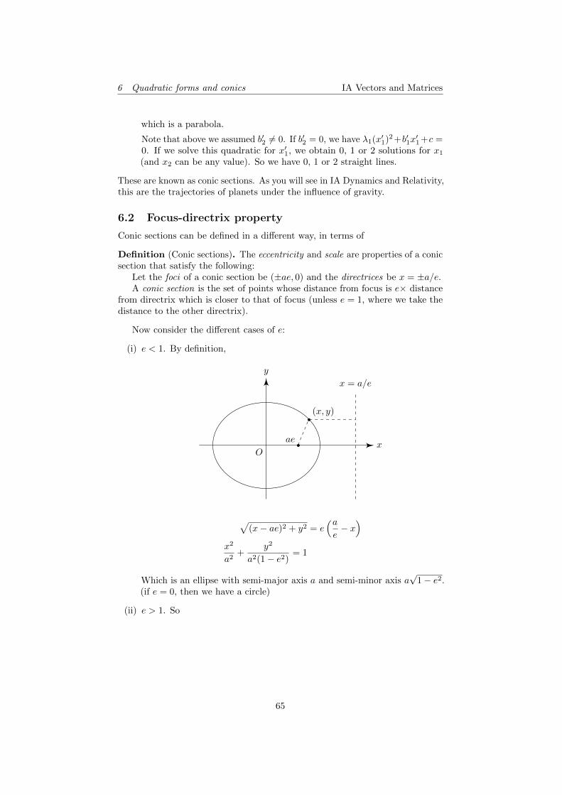
6 Quadratic forms and conics IA Vectors and Matrices
which is a parabola.
Note that above we assumed b′2 6= 0. If b′2 = 0, we have λ1(x′1)2 +b′1x′1 +c =
0. If we solve this quadratic for x′1, we obtain 0, 1 or 2 solutions for x1
(and x2 can be any value). So we have 0, 1 or 2 straight lines.
These are known as conic sections. As you will see in IA Dynamics and Relativity,this are the trajectories of planets under the influence of gravity.
6.2 Focus-directrix property
Conic sections can be defined in a different way, in terms of
Definition (Conic sections). The eccentricity and scale are properties of a conicsection that satisfy the following:
Let the foci of a conic section be (±ae, 0) and the directrices be x = ±a/e.A conic section is the set of points whose distance from focus is e× distance
from directrix which is closer to that of focus (unless e = 1, where we take thedistance to the other directrix).
Now consider the different cases of e:
(i) e < 1. By definition,
x
y
O
x = a/e
ae
(x, y)
√(x− ae)2 + y2 = e
(ae− x)
x2
a2+
y2
a2(1− e2)= 1
Which is an ellipse with semi-major axis a and semi-minor axis a√
1− e2.(if e = 0, then we have a circle)
(ii) e > 1. So
65

6 Quadratic forms and conics IA Vectors and Matrices
x
y
O
x = a/e
ae
(x, y)
√(x− ae)2 + y2 = e
(x− a
e
)x2
a2− y2
a2(e2 − 1)= 1
and we have a hyperbola.
(iii) e = 1: Then
x
y
O
x = a
a
(x, y)
√(x− a)2 + y2 = (x+ 1)
y2 = 4ax
and we have a parabola.
Conics also work in polar coordinates. We introduce a new parameter l suchthat l/e is the distance from the focus to the directrix. So
l = a|1− e2|.
66

6 Quadratic forms and conics IA Vectors and Matrices
We use polar coordinates (r, θ) centered on a focus. So the focus-directrixproperty is
r = e
(l
e− r cos θ
)r =
l
1 + e cos θ
We see that r → ∞ if θ → cos−1(−1/e), which is only possible if e ≥ 1, i.e.hyperbola or parabola. But ellipses have e < 1. So r is bounded, as expected.
67

7 Transformation groups IA Vectors and Matrices
7 Transformation groups
We have previously seen that orthogonal matrices are used to transform betweenorthonormal bases. Alternatively, we can see them as transformations of spaceitself that preserve distances, which is something we will prove shortly.
Using this as the definition of an orthogonal matrix, we see that our definitionof orthogonal matrices is dependent on our choice of the notion of distance, ormetric. In special relativity, we will need to use a different metric, which willlead to the Lorentz matrices, the matrices that conserve distances in specialrelativity. We will have a brief look at these as well.
7.1 Groups of orthogonal matrices
Proposition. The set of all n× n orthogonal matrices P forms a group undermatrix multiplication.
Proof.
0. If P,Q are orthogonal, then consider R = PQ. RRT = (PQ)(PQ)T =P (QQT )PT = PPT = I. So R is orthogonal.
1. I satisfies IIT = I. So I is orthogonal and is an identity of the group.
2. Inverse: if P is orthogonal, then P−1 = PT by definition, which is alsoorthogonal.
3. Matrix multiplication is associative since function composition is associative.
Definition (Orthogonal group). The orthogonal group O(n) is the group oforthogonal matrices.
Definition (Special orthogonal group). The special orthogonal group is thesubgroup of O(n) that consists of all orthogonal matrices with determinant 1.
In general, we can show that any matrix in O(2) is of the form(cos θ − sin θsin θ cos θ
)or
(cos θ sin θsin θ − cos θ
)
7.2 Length preserving matrices
Theorem. Let P ∈ O(n). Then the following are equivalent:
(i) P is orthogonal
(ii) |Px| = |x|
(iii) (Px)T (Py) = xTy, i.e. (Px) · (Py) = x · y.
(iv) If (v1,v2, · · · ,vn) are orthonormal, so are (Pv1, Pv2, · · · , Pvn)
(v) The columns of P are orthonormal.
Proof. We do them one by one:
68
7 Transformation groups IA Vectors and Matrices
(i) ⇒ (ii): |Px|2 = (Px)T (Px) = xTPTPx = xTx = |x|2
(ii) ⇒ (iii): |P (x + y)|2 = |x + y|2. The right hand side is
(xT + yT )(x + y) = xTx + yTy + yTx + xTy = |x|2 + |y|2 + 2xTy.
Similarly, the left hand side is
|Px + Py|2 = |Px|2 + |Py|+ 2(Px)TPy = |x|2 + |y|2 + 2(Px)TPy.
So (Px)TPy = xTy.
(iii) ⇒ (iv): (Pvi)TPvj = vTi vj = δij . So Pvi’s are also orthonormal.
(iv) ⇒ (v): Take the vi’s to be the standard basis. So the columns of P , beingPei, are orthonormal.
(v) ⇒ (i): The columns of P are orthonormal. Then (PPT )ij = PikPjk =(Pi) · (Pj) = δij , viewing Pi as the ith column of P . So PPT = I.
Therefore the set of length-preserving matrices is precisely O(n).
7.3 Lorentz transformations
Consider the Minkowski 1 + 1 dimension spacetime (i.e. 1 space dimension and1 time dimension)
Definition (Minkowski inner product). The Minkowski inner product of 2vectors x and y is
〈x | y〉 = xTJy,
where
J =
(1 00 −1
)Then 〈x | y〉 = x1y1 − x2y2.
This is to be compared to the usual Euclidean inner product of x,y ∈ R2,given by
〈x | y〉 = xTy = xT Iy = x1y1 + x2y2.
Definition (Preservation of inner product). A transformation matrix M pre-serves the Minkowski inner product if
〈x|y〉 = 〈Mx|My〉
for all x,y.
We know that xTJy = (Mx)TJMy = xTMTJMy. Since this has to betrue for all x and y, we must have
J = MTJM.
We can show that M takes the form of
Hα =
(coshα sinhαsinhα coshα
)or Kα/2 =
(coshα − sinhαsinhα − coshα
)
69

7 Transformation groups IA Vectors and Matrices
where Hα is a hyperbolic rotation, and Kα/2 is a hyperbolic reflection.This is technically all matrices that preserve the metric, since these only
include matrices with M11 > 0. In physics, these are the matrices we want, sinceM11 < 0 corresponds to inverting time, which is frowned upon.
Definition (Lorentz matrix). A Lorentz matrix or a Lorentz boost is a matrixin the form
Bv =1√
1− v2
(1 vv 1
).
Here |v| < 1, where we have chosen units in which the speed of light is equal to1. We have Bv = Htanh−1 v
Definition (Lorentz group). The Lorentz group is a group of all Lorentz matricesunder matrix multiplication.
It is easy to prove that this is a group. For the closure axiom, we haveBv1Bv2 = Bv3 , where
v3 = tanh(tanh−1 v1 + tanh−1 v2) =v1 + v2
1 + v1v2
The set of all Bv is a group of transformations which preserve the Minkowskiinner product.
70