Part 1: The 2D projective plane and it’s applications Martin Jagersand CMPUT 613 Non-Euclidean...

Part 1:Part 1:

The 2D projective plane and The 2D projective plane and it’s applicationsit’s applications

Martin JagersandMartin Jagersand

CMPUT 613Non-Euclidean Geometry

forComputer Vision

Why geometry?

X

Y

Z

HZ

Xx

=

x

y

Scene structureImage structure

= =

x

X

X

YfZ

Richard Hartley and Andrew Zisserman, Multiple View Geometry, Cambridge University Publishers, 2nd ed. 2004

2D Geometry readings: Ch1: Cursorly

Ch 2.1-4, 2.7, Ch 4.1-4.2.5, 4.4.4-4.8 cursorly

Modeling from images

Cam

era(

s)

Scene structure ImageImage

StructureWorld

model-based renderingimage-based modeling

image-based rendering

Tra

ckin

g &

SF

M

Cam

era(

s)

What 2d and 3d representations best support this process?

Euclidean Geometry?

• Is Euclidean geometry needed?Is Euclidean geometry needed? RenderingRendering: requires only model : requires only model reprojectionreprojection

RoboticsRobotics: control via image feature alignments: control via image feature alignments

•Rendering: Rendering: pixel reprojectionpixel reprojection

•Robotics: Robotics: visual servoingvisual servoing

Euclidean model needed?

Euclidean Geometry?

• Is Euclidean geometry needed?Is Euclidean geometry needed? RenderingRendering: requires model : requires model reprojectionreprojection

RoboticsRobotics: control via image feature alignments: control via image feature alignments

•Euclidean model: Euclidean model: ++ describes the real world of objects/scenes describes the real world of objects/scenes

++ quite natural for most people to work with quite natural for most people to work with (everyday relationships, angles, distances, …)(everyday relationships, angles, distances, …)

- difficult to extract from images- difficult to extract from images (camera is not a Euclidean measuring device)(camera is not a Euclidean measuring device)

x

yX

YfZ=

nonlinear…

X

Y

Z

What images don’t provide

Rendering’s inverseRendering’s inverse

lengths

depth


Multiple views…

left

right


Multiple views…

left

right

above

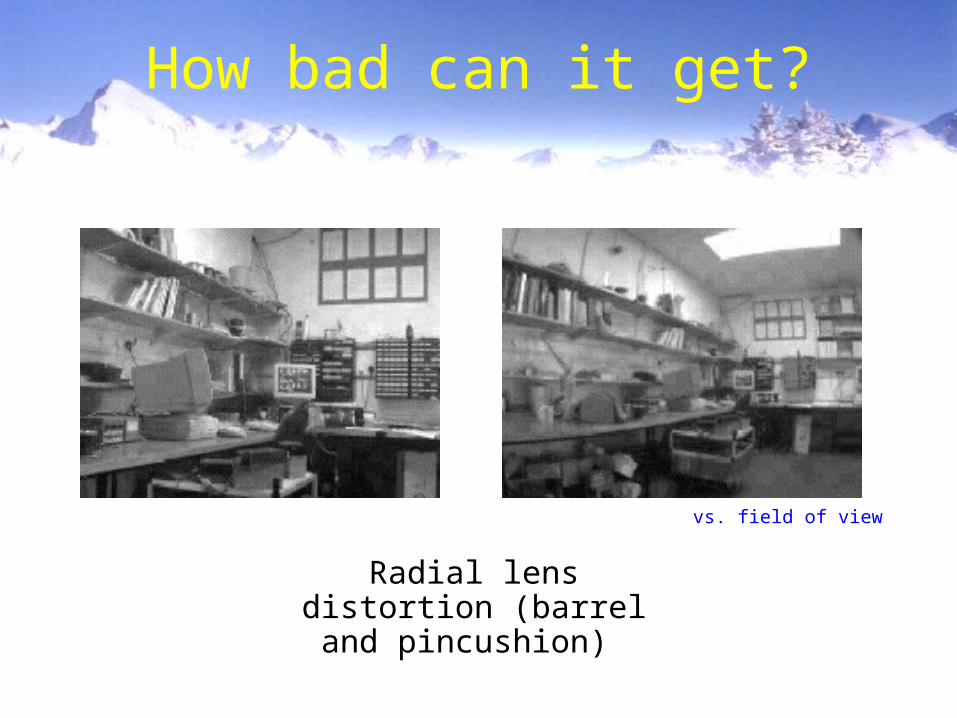
How bad can it get?

Radial lens distortion (barrel and pincushion)

vs. field of view

Correcting Lens Distortion

Distortion model

Parameter estimation

reference features

“corrected” image

Tsai ’87; Brand, Mohr, Bobet ’94

X

Y

Z

Homogeneous coordinates

X

Y

Z

s

s 0

X∞

X

Y

0

X∞ =

• Perspective imaging models 2d projective space

• Each 3D ray is a point in P2 : homogeneous coords.

• Ideal points

• P2 is R2 plus a “line at infinity” l∞

The 2D projective plane

Projective point

l∞

x

yX

Y1Z= Inhomogeneou

s equivalent

Lines

HZ • Ideal line ~ the plane parallel to the image

A

B

C

l =X=lTX = XTl = AX + BY + CZ = 0

l∞ =

0

0

1

• Projective line ~ a plane through the origin

For any 2d projective property, a dual property holds when the role of points and lines are interchanged.

Duality:

X

Y

0

X∞ =

l1 l2X =X1 X2=l

The line joining two points The point joining two lines

X

Y

Z

X

l“line at infinity

”

AX + BY + C = 0

Conics

•Conic: Conic: – Euclidean geometry: hyperbola, ellipse, parabola & degenerateEuclidean geometry: hyperbola, ellipse, parabola & degenerate– Projective geometry: equivalent under projective transformProjective geometry: equivalent under projective transform– Defined by 5 pointsDefined by 5 points

•Tangent lineTangent line

•Dual conic C*Dual conic C*

0

022

xx C

feydxcybxyaxT

fed

ecb

dba

C

2/2/

2/2/

2/2/

xl C

0* ll CT

inhomogeneous

homogeneous

Projective transformations

• Homographies, collineations, projectivitiesHomographies, collineations, projectivities

• 3x3 nonsingular H3x3 nonsingular H

3

2

1

333231

232221

131211

3

2

1

'

'

'

x

x

x

hhh

hhh

hhh

x

x

x

l0= Hà Tl

xTl = 0 x0Tl0= 0

maps P2 to P2

8 degrees of freedomdetermined by 4 corresponding points

x0= Hx• Transforming Lines?subspaces preserved:pts on line remain on line

xTHTHà Tl = 0substitution

dual transformationxTHTl0= 0

Planar Projective Warping

HZA novel view rendered via

four points with known structurexi

0= Hxii = 1. . .4

xi xi0

Planar Projective Warping

HZOriginal Top-down Facing right

Artifacts are apparent where planarity is violated...

2d Homographies

2 images of a plane

2 images from the same viewpoint (Perspectivity)

Panoramic imagingAppl: Quicktime VR, robot navigation etc.

Homographies of the world, unite!

Image mosaics

HZ

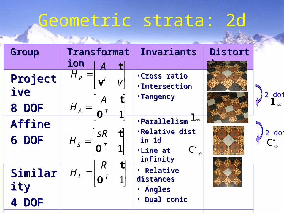
GroupGroup TransformationTransformation InvariantsInvariants DistortionDistortion

ProjectiveProjective

8 DOF8 DOF

• Cross ratioCross ratio

• IntersectionIntersection

• TangencyTangency

AffineAffine

6 DOF6 DOF

• ParallelismParallelism

• Relative dist in 1dRelative dist in 1d

• Line at infinityLine at infinity

SimilaritySimilarity

4 DOF4 DOF

• Relative distancesRelative distances

• AnglesAngles

• Dual conicDual conic

EuclideanEuclidean

3 DOF3 DOF

• LengthsLengths

• AreasAreas

Geometric strata: 2d

1TS

sRH

O

t

1TA

AH

O

t

1TE

RH

O

t

v

AH TP v

t

C*

2 dofl

2 dof

l

C*

The line at infinity

l

1

0

0

1t

0ll

TT

TT

A

AH A

HZ 2:17: The line at infinity l is a fixed line under a projective transformation H if and only if H is an

affinity

Note: But points on l can be rearranged to new points on l

Affine properties from images

Projection(Imaging)

RectificationPost-processing

Affine rectification

v1 v2

l1

l2 l4

l3

l∞21 vvl

211 llv 432 llv

APA

lll

HH

321

010

001

0,l 3321 llll T

Point transformation for Aff Rect:

Exercise: Verify

T321 lll

TT ]1,0,0[321 lllTPAH

Math tools 1:Solving Linear Systems

• If If mm == nn ( (AA is a square matrix), then we can obtain is a square matrix), then we can obtain the solution by simple inversion:the solution by simple inversion:

• If If mm >> nn, then the system is , then the system is over-constrainedover-constrained and and

AA is not invertible is not invertible – Use Matlab “\” to obtain Use Matlab “\” to obtain least-squares solutionleast-squares solution xx == A\b A\b to to Ax Ax

=b =b internally Matlab uses QR-factorization (cmput340) to solve this.internally Matlab uses QR-factorization (cmput340) to solve this. – Can also write this using pseudoinverse Can also write this using pseudoinverse AA+ + == ((AATTAA))-1-1AATT to obtain to obtain

least-squares solutionleast-squares solution xx == A A++bb

Fitting Lines

• A 2-D point A 2-D point xx = ( = (xx, , yy)) is on a line with slope is on a line with slope

mm and intercept and intercept bb if and only if if and only if yy = = mxmx + + bb • Equivalently,Equivalently,

• So the line defined by two points So the line defined by two points xx11, , xx22 is the is the

solution to the following system of equations:solution to the following system of equations:

Fitting Lines

• With more than two points, there is no guarantee With more than two points, there is no guarantee that they will all be on the same linethat they will all be on the same line

• Least-squares solution obtained from Least-squares solution obtained from pseudoinverse is line that is “closest” to all of the pseudoinverse is line that is “closest” to all of the pointspoints

courtesy ofVanderbilt U.

Example: Fitting a Line

• Suppose we have points Suppose we have points (2, 1)(2, 1), , (5, 2)(5, 2), , (7, (7, 3)3), and , and (8, 3)(8, 3)

• Then Then

and and x x == A A++b b == (0.3571, 0.2857)(0.3571, 0.2857)TT

Matlab: Matlab: x x == A\b A\b

Example: Fitting a Line

Homogeneous Systems of Equations

• Suppose we want to solve Suppose we want to solve AA x = 0x = 0• There is a trivial solution There is a trivial solution x = 0x = 0, but we don’t want , but we don’t want

this. For what other values of this. For what other values of xx is is AA xx close to close to 00??• This is satisfied by computing the This is satisfied by computing the singular value singular value

decompositiondecomposition (SVD) (SVD) A A == UDV UDVTT (a non- (a non-negative diagonal matrix between two orthogonal negative diagonal matrix between two orthogonal matrices) and taking matrices) and taking xx as the last column of as the last column of VV– Note that Matlab returns Note that Matlab returns [U, D, V] = svd(A)[U, D, V] = svd(A)

Line-Fitting as a Homogeneous System

• A 2-D homogeneous point A 2-D homogeneous point xx = ( = (xx, , yy, 1), 1)TT is on is on

the line the line ll = ( = (aa, , bb, , cc))TT only when only when

axax + + byby + + cc = 0 = 0• We can write this equation with a dot product: We can write this equation with a dot product:

x•x• ll = 0 = 0,, and hence the following system is and hence the following system is

implied for multiple points implied for multiple points xx11,, x x22, ..., , ..., xxnn::

Example: Homogeneous Line-Fitting

• Again we have 4 points, but now in homogeneous form: Again we have 4 points, but now in homogeneous form:

(2, 1, 1)(2, 1, 1), , (5, 2, 1)(5, 2, 1), , (7, 3, 1)(7, 3, 1), and , and (8, 3, 1)(8, 3, 1)• Our system is:Our system is:

• Taking the SVD of Taking the SVD of AA, we get:, we get:compare to x = (0.3571, 0.2857)T

Parameter estimation in geometric transforms

•2D homography2D homographyGiven a set of (xGiven a set of (xii,x,xii’), compute H (x’), compute H (xii’=Hx’=Hxii))

•3D to 2D camera projection3D to 2D camera projectionGiven a set of (XGiven a set of (Xii,x,xii), compute P (x), compute P (xii=PX=PXii))

•Fundamental matrixFundamental matrixGiven a set of (xGiven a set of (xii,x,xii’), compute F ’), compute F (x(xii’’TTFxFxii=0)=0)

•Trifocal tensor Trifocal tensor Given a set of (xGiven a set of (xii,x,xii’,x’,xii”), compute T”), compute T

Now

Estimating Homography Hgiven image points x

HZA novel view rendered via

four points with known structurexi

0= Hxii = 1. . .4

xi xi0

Number of measurements required

• At least as many independent equations as degrees of At least as many independent equations as degrees of freedom requiredfreedom required

• Example: Example:

Hxx'

1'

λ

333231

232221

131211

y

x

hhh

hhh

hhh

w

y

x

2 independent equations / point8 degrees of freedom

4x2≥8

Approximate solutions

•Minimal solutionMinimal solution4 points yield an exact solution for H4 points yield an exact solution for H

•More pointsMore points– No exact solution, because measurements are inexact No exact solution, because measurements are inexact

(“noise”)(“noise”)– Search for “best” according to some cost functionSearch for “best” according to some cost function– Algebraic or geometric/statistical costAlgebraic or geometric/statistical cost

Many ways to solve:

Different Cost functions => differencesDifferent Cost functions => differencesin solution in solution

•Algebraic distanceAlgebraic distance

•Geometric distanceGeometric distance

•Reprojection errorReprojection error

•ComparisonComparison

•Geometric interpretationGeometric interpretation

Gold Standard algorithm

•Cost function that is optimal for some Cost function that is optimal for some assumptionsassumptions

•Computational algorithm that minimizes it is Computational algorithm that minimizes it is called “Gold Standard” algorithm called “Gold Standard” algorithm

•Other algorithms can then be compared to itOther algorithms can then be compared to it

Estimating H: The Direct Linear Transformation (DLT) Algorithm

• xxi i =H=HXXii is an equation involving homogeneous is an equation involving homogeneous

vectors, so vectors, so HHXXii and and xxi i need only be in the same need only be in the same

direction, not strictly equaldirection, not strictly equal

• We can specify “same directionality” by using a We can specify “same directionality” by using a cross product formulation:cross product formulation:

0Hxx ii

Direct Linear Transformation(DLT)

ii Hxx 0Hxx ii

i

i

i

i

xh

xh

xh

Hx3

2

1

T

T

T

iiii

iiii

iiii

ii

yx

xw

wy

xhxh

xhxh

xhxh

Hxx12

31

23

TT

TT

TT

0

h

h

h

0xx

x0x

xx0

3

2

1

TTT

TTT

TTT

iiii

iiii

iiii

xy

xw

yw

Tiiii wyx ,,x

0hA i


• Equations are linear in Equations are linear in hh

0

h

h

h

0xx

x0x

xx0

3

2

1

TTT

TTT

TTT

iiii

iiii

iiii

xy

xw

yw

0hA i

• Only 2 out of 3 are linearly independent Only 2 out of 3 are linearly independent

(indeed, 2 eq/pt)(indeed, 2 eq/pt)

0

h

h

h

x0x

xx0

3

2

1

TTT

TTT

iiii

iiii

xw

yw

(only drop third row if wi’≠0)• Holds for any homogeneous representation, Holds for any homogeneous representation,

e.g. (e.g. (xxii’,’,yyii’,1)’,1)


•Solving for Solving for HH

0Ah 0h

A

A

A

A

4

3

2

1

size A is 8x9 or 12x9, but rank 8

Trivial solution is h=09T is not interesting

1-D null-space yields solution of interestpick for example the one with 1h


•Over-determined solutionOver-determined solution

No exact solution because of inexact measurementi.e. “noise”

0Ah 0h

A

A

A

n

2

1

Find approximate solution- Additional constraint needed to avoid 0, e.g.

- not possible, so minimize

1h Ah0Ah

DLT algorithm

ObjectiveGiven n≥4 2D to 2D point correspondences {xi↔xi’}, determine the 2D homography matrix H such that xi’=Hxi

Algorithm

(i) For each correspondence xi ↔xi’ compute Ai. Usually only two first rows needed.

(ii) Assemble n 2x9 matrices Ai into a single 2nx9 matrix A

(iii) Obtain SVD of A. Solution for h is last column of V

(iv) Determine H from h (reshape)

Inhomogeneous solution

'

'h~

''000'''

'''''000

ii

ii

iiiiiiiiii

iiiiiiiiii

xw

yw

xyxxwwwywx

yyyxwwwywx

Since h can only be computed up to scale, pick hj=1, e.g. h9=1, and solve for 8-vector

h~

Solve using Gaussian elimination (4 points) or using linear least-squares (more than 4 points)

However, if h9=0 this approach fails also poor results if h9 close to zeroTherefore, not recommended for general homographiesNote h9=H33=0 if origin is mapped to infinity

0

1

0

0

H100Hxl 0

T

Normalizing transformations

• Since DLT is not invariant to coordinate Since DLT is not invariant to coordinate transforms, what is a good choice of transforms, what is a good choice of coordinates?coordinates?e.g.e.g.– Translate centroid to originTranslate centroid to origin– Scale to a average distance to the originScale to a average distance to the origin– Independently on both imagesIndependently on both images

2

1

norm

100

2/0

2/0

T

hhw

whwOr

Normalized DLT algorithm

ObjectiveGiven n≥4 2D to 2D point correspondences {xi↔xi’}, determine the 2D homography matrix H such that xi’=Hxi

Algorithm

(i) Normalize points

(ii) Apply DLT algorithm to

(iii) Denormalize solution

,x~x~ ii inormiinormi xTx~,xTx~

norm-1

norm TH~

TH

Importance of normalization

0

h

h

h

0001

1000

3

2

1

iiiiiii

iiiiiii

xyxxxyx

yyyxyyx

~102 ~102 ~102 ~102 ~104 ~104 ~10211

orders of magnitude difference!

Degenerate configurations

x4

x1

x3

x2

x4

x1

x3

x2H? H’?

x1

x3

x2

x4

0Hxx iiConstraints: i=1,2,3,4

TlxH 4* Define:

4444* xxlxxH kT

3,2,1 ,0xlxxH 4* iii

TThen,

H* is rank-1 matrix and thus not a homography

(case A) (case B)

If H* is unique solution, then no homography mapping xi→xi’(case B)

If further solution H exist, then also αH*+βH (case A) (2-D null-space in stead of 1-D null-space)

short and long focal length

Radial Distortion

Radial Distortion

Correction of distortion

Choice of the distortion function and center

Computing the parameters of the distortion function(i) Minimize with additional unknowns(ii) Straighten lines(iii) …

Radial Distortion

Part 1: The 2D projective plane and it’s applications Martin Jagersand CMPUT 613 Non-Euclidean...

Documents

Transcript of Part 1: The 2D projective plane and it’s applications Martin Jagersand CMPUT 613 Non-Euclidean...