Parsing IKEA Objects: Fine Pose Estimation

Joseph J. Lim Hamed Pirsiavash Antonio TorralbaMassachusetts Institute of Technology

Compter Science and Artificial Intelligence Laboratory{lim,hpirsiav,torralba}@csail.mit.edu

Abstract

We address the problem of localizing and estimating thefine-pose of objects in the image with exact 3D models. Ourmain focus is to unify contributions from the 1970s with re-cent advances in object detection: use local keypoint de-tectors to find candidate poses and score global alignmentof each candidate pose to the image. Moreover, we alsoprovide a new dataset containing fine-aligned objects withtheir exactly matched 3D models, and a set of models forwidely used objects. We also evaluate our algorithm bothon object detection and fine pose estimation, and show thatour method outperforms state-of-the art algorithms.

1. IntroductionJust as a thought experiment imagine that we want to

detect and fit 3D models of IKEA furniture in the imagesas shown in Figure 1. We can find surprisingly accurate3D models of IKEA furniture, such as billy bookcase andektorp sofa, created by IKEA fans from Google 3D Ware-house and other publicly available databases. Therefore,detecting those models in images could seem to be a verysimilar task to an instance detection problem in which wehave training images of the exact instance that we want todetect. But, it is not exactly like detecting instances. In thecase of typical 3D models (including IKEA models fromGoogle Warehouse), the exact appearance of each piece isnot available, only the 3D shape is. Moreover, appearancein real images will vary significantly due to a number offactors. For instance, IKEA furniture might appear withdifferent colors and textures, and with geometric deforma-tions (as people building them might not do it perfectly) andocclusions (e.g., a chair might have a cushion on top of it).

The problem that we introduce in this paper is detect-ing and accurately fitting exact 3D models of objects to realimages, as shown in Figure 1. Detecting 3D objects in im-ages and estimating their pose was a popular topic in theearly days of computer vision [14] and has gained a renewedinterest in the last few years. The traditional approaches

3D Model Original Image Fine-pose Estimation

Figure 1. Our goal in this paper is to detect and estimate the fine-pose of an object in the image given an exact 3D model.

[12, 14] were dominated by using accurate geometric rep-resentations of 3D objects with an emphasis on viewpointinvariance. Objects would appear in almost any pose andorientation in the image. Most of the approaches were de-signed to work at instance level detection as it was expectedthat the 3D model would accurately fit the model in the im-age. Instance level detection regained interest with the in-troduction of new invariant local descriptors that dramati-cally improved the detection of interest points [17]. Thosemodels assumed knowledge about geometry and appear-ance of the instance. Having access to accurate knowledgeabout those two aspects allowed precise detections and poseestimations of the object on images even in the presence ofclutter and occlusions.

In the last few years, researchers interested in category

1

Edgemap HOG Local correspondence deteciton Image

Figure 2. Local correspondence: for each 3D interest point Xi (red, green, and blue), we train an LDA patch detector on an edgemapand use its response as part of our cost function. We compute HOG on edgemaps to ensure a real image and our model share the modality.

level detection have extended 2D constellation models to in-clude 3D information in the object representation. Many ofthese models [9, 20, 10, 6, 5, 19, 16, 7, 21] rely on gradient-based features [1, 13]. Category level detection requires themodels to be generic and flexible, as they have to deal withall the variations in shape and appearance of the instancesthat belong to the same category. Therefore, the shape rep-resentations used for those models are coarse (e.g., modeledas the constellation of a few 3D parts or planes) and the ex-pected output is at best an approximate fitting of the 3Dmodel to the image.

In this paper we introduce a detection task that is in theintersection of these two settings; it is more generic thandetecting instances, but we assume richer models than theones typically used in category level detection. In particu-lar, we assume that accurate CAD models of the objects areavailable. Hence, there is little variation on the shape of theinstances that form one category. However, there might belarge variation in the appearance, as the CAD models do notcompletely constrain the appearance of the objects placedin the real world. Although assuming that CAD models areavailable might seem to be a restrictive assumption, thereare available 3D CAD models for most man-made artifacts,used for manufacturing or virtual reality. All those mod-els could be used as training data for our system. Hence,we focus on detection and pose estimation of objects in thewild given their 3D CAD models. Our goal is to provide anaccurate localization of the object, as in the instance leveldetection problem, but dealing with some of the variabilitythat one finds in category level detection.

Our contributions are three folds: (1) Proposing a detec-tion problem that has some of the challenges of categorylevel detection while allowing for an accurate representa-tion of the object pose in the image. This problem will mo-tivate the development of better 3D object models and thealgorithms needed to find them in images. (2) We proposea novel solution that unifies contributions from the 1970s

with recent advances in object detection. (3) And we in-troduce a new dataset of 3D IKEA models obtained fromGoogle Warehouse and real images containing instances ofIKEA furniture and annotated with ground truth pose.

2. MethodsWe now propose the framework that can detect objects

and estimate their poses simultaneously by matching to oneof the 3D models in our database.

2.1. Our ModelThe core of our algorithm is to define the final score

based on multiple sources of information such as localcorrespondence, geometric distance, and global alignment.Suppose we are given the image I containing an object forwhich we want to estimate the projection matrix P with 9degrees of freedom 1. We define our cost function S withthree terms as follows:

S(P, c) = L(P, c) + wDD(P, c) + wGG(P ) (1)

where c refers to the set of correspondences, L measures er-ror in local correspondences between the 3D model and 2Dimage, D measures geometric distance between correspon-dences in 3D, and G measures the global dissimilarity in2D. Note that we designed our model to be linear in weightvectors of wD and wG. We will use this linearity later tolearn our discriminative classifier.

2.2. Local correspondence errorThe goal here is to measure the local correspondences.

Given a projection P , we find the local shape-based match-ing score between the rendered image of the CAD modeland the 2D image. Because our CAD model contains only

1We assume the image is captured by a regular pinhole camera and isnot cropped, so the the principal point is in the middle of image.

shape information, a simple distance measure on standardlocal descriptors fails to match the two images. In orderto overcome this modality difference, we compute HOG onthe edgemap of both images since it is more robust to ap-pearance change but still sensitive to the change in shape.Moreover, we see better performance by training an LDAclassifier to discriminate each keypoint from the rest of thepoints. This is equivalent to a dot product between descrip-tors in the whitened space. One advantage of using LDAis its high training speed compared to other previous HOG-template based approaches. Figure 2 illustrates this step.

More formally, our correspondence error is measured by

L(P, c) =X

i

H(�Ti �(xci)� ↵) (2)

�i = ⌃

�1(�(P (Xi))� µ) (3)

where �i is the weight learned using LDA based on thecovariance ⌃ and mean µ obtained from a large externaldataset [8], �(·) is a HOG computed on a 20⇥20 pixeledgemap patch of a given point, xci is the 2D correspond-ing point of 3D point Xi, P (·) projects a 3D point to 2Dcoordinate given pose P , and lastly H(x � ↵) binarizes xto 0 if x � ↵ or to 1 otherwise.

2.3. Geometric distance between correspondencesGiven a proposed set of correspondences c between the

CAD model and the image, it is also necessary to measure ifc is a geometrically acceptable pose based on the 3D model.For the error measure, we use euclidean distance betweenthe projection of xi and its corresponding 2D point xci ; aswell as the line distance defined in [12] between the 3D linel and its corresponding 2D line cl.

D(P,c) =X

i2V

kP (Xi)� xcik2+ (4)

X

l2L

����

cos�cl , sin�cl ,�⇢cl

� P (Xl1) P (Xl2)

1 1

� ����2

where Xl1 and Xl2 are end points of line l, and �cl and ⇢clare polar coordinate parameters of line cl.

The first term measures a pairwise distance between a 3Dinterest point Xi and its 2D corresponding point xci . Thesecond term measures the alignment error between a 3D in-terest line l and one of its corresponding 2D lines cl [12].We use the Hough transform on edges to extract 2D linesfrom I . Note that this cost does not penalize displacementalong the line. This is important because the end pointsof detected lines on I are not reliable due to occlusion andnoise in the image.

2.4. Global dissimilarityOne key improvement of our work compared to tradi-

tional works on pose estimation using a 3D model is how

we measure the global alignment. We use recently devel-oped features to measure the global alignment between ourproposal and the image:

G(P ) = [fHOG, fregion, fedge, fcorr, ftexture], (5)

The description of each feature follows:

HOG-based: While D and L from Eq 1 are designed tocapture fine local alignments, the local points are sparse andhence it is yet missing an object-scale alignment. In orderto capture edge alignment per orientation, we compute afine HOG descriptor (2x2 per cell) of edgemaps of I andthe rendered image of pose P . We use a similarity measurebased on cosine similarity between vectors .

fHOG =

�(I)T�(P )

k�(P )k2 ,�(I)T�(P )

k�(I)Mk2 ,

�(I)T�(P )

k�(I)Mkk�(P )k

�, (6)

where �(·) is a HOG descriptor and M is a mask matrixfor counting how many pixels of P fall into each cell. Wemultiply �(I) by M to normalize only within the proposedarea (by P ) without being affected by other area.

Regions: We add another alignment feature based on super-pixels. If our proposal P is a reasonable candidate, super-pixels should not cross over the object boundary, except inheavily occluded areas. To measure this spill over, we firstextract super-pixels, RI , from I using [3] and compute aratio between an area of a proposed pose, |RP |, and an areaof regions that has some overlap with RP . This ratio willcontrol the spillover effect as shown in Figure 3.

(a) Original image (b) Candidate 1 (c) Candidate 2Figure 3. Region feature: One feature to measure a fine align-ment is the ratio between areas of a proposed pose (yellow) andregions overlapped with the proposed pose. (a) is an original im-age I , and (b) shows an example to encourage, while (c) shows anexample to penalize.

fregion =

"P|RP\RI |>0.1|RP | |RP |

|RI |

#(7)

Texture boundary: The goal of this feature is to captureappearance by measuring how well our proposed pose sep-arates object boundary. In other words, we would like to

measure the alignment between the boundary of our pro-posed pose P and the texture boundary of I . For this pur-pose, we use a well-known texture classification feature,Local Binary Pattern (LBP) [15].

We compute histograms of LBP on inner boundary andouter boundary of proposed pose P . We define an innerboundary region by extruding the proposed object maskfollowed by subtracting the mask, and an outer boundaryby diluting the proposed object mask. Essentially, the his-tograms will encode the texture patterns of near-inner/outerpixels along the proposed pose P ’s boundary. Hence, alarge change in these two histograms indicates a largetexture pattern change, and it is ideal if the LBP histogramdifference along the proposed pose’s boundary is large.This feature will discourage the object boundary aligningwith contours with small texture change (such as contourswithin an object or contours due to illumination).

Edges: We extract edges [11] from the image to measuretheir alignment with the edgemap of estimated pose. Weused a modified Chamfer distance from Satkin, et. al. [18].

fedge =

1

|R|X

a2R

min(min

b2Ika� bk, ⌧),

1

|I|X

b2I

min(min

a2Rkb� ak, ⌧)

�(8)

where we use ⌧ 2 {10, 25, 50,1} to control the influenceof outlier edges.

Number of correspondences: fcorr is a binary vector,where the i’th dimension indicates if there are more than igood correspondences between the 3D model and the 2Dimage under pose P . Good correspondences are the oneswith local correspondence error (in Eq 2) below a threshold.

2.5. Optimization & Learning

Algorithm 1 Pose set {P} searchFor each initial seed pose,while less than n different candidates found do

Choose a random 3D interest point and its 2D corre-spondence (this determines a displacement)for i = 1 to 5 do

Choose a random local correspondence agreeingwith correspondences selected (over i�1 iterations)

end forEstimate parameters by solving least squaresFind all correspondences agreeing with this solutionEstimate parameters using all correspondences

end while

Our cost function S(P, c) from Eq 1 with G(P ) is a non-convex function and is not easy to solve directly. Hence,we first simplify the optimization by quantizing the spaceof solutions. Because our L(P, c) is 1 if any local corre-spondence score is below the threshold, we first find all setsof correspondences for which all local correspondences areabove the threshold. Then, we find the pose P that mini-mizes L(P, c) + wD

(P, c). Finally, we optimize the costfunction in the discrete space by evaluating all candidates.

We use RANSAC in populating a set of candidates byoptimizing L(P, c). Our RANSAC procedure is shown inAlg 1. We then minimize L(P, c) + wDD(P, c) by esti-mating pose P for each found correspondence c. Givena set of correspondences c, we estimate pose P using theLevenberg-Marquardt algorithm minimizing D(P, c).

We again leverage the discretized space from Alg 1 inorder to learn weights for Eq 1. For the subset of {(P, c)}in the training set, we extract the geometric distance andglobal alignment features,

⇥D(P, c), G(P )

⇤, and the binary

labels based on the distance from the ground truth (definedin Eq 9) . Then, we learn the weights using a linear SVMclassifier.

3. Evaluation3.1. Dataset

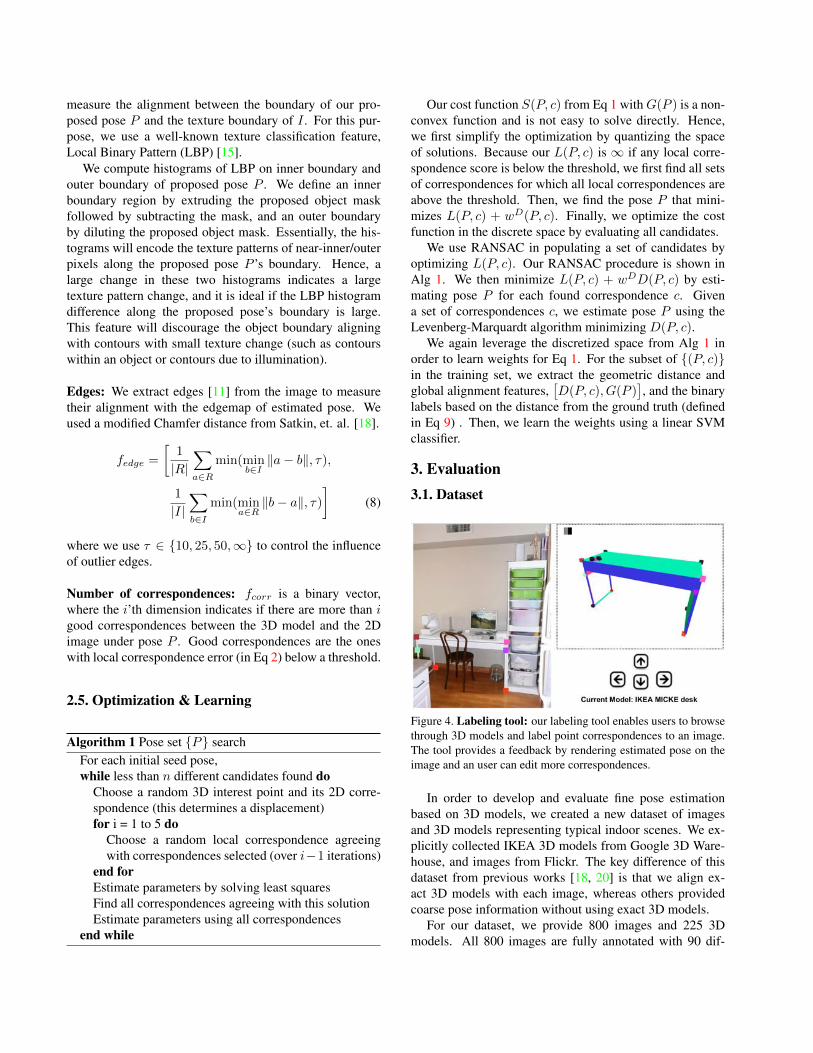
Figure 4. Labeling tool: our labeling tool enables users to browsethrough 3D models and label point correspondences to an image.The tool provides a feedback by rendering estimated pose on theimage and an user can edit more correspondences.

In order to develop and evaluate fine pose estimationbased on 3D models, we created a new dataset of imagesand 3D models representing typical indoor scenes. We ex-plicitly collected IKEA 3D models from Google 3D Ware-house, and images from Flickr. The key difference of thisdataset from previous works [18, 20] is that we align ex-act 3D models with each image, whereas others providedcoarse pose information without using exact 3D models.

For our dataset, we provide 800 images and 225 3Dmodels. All 800 images are fully annotated with 90 dif-

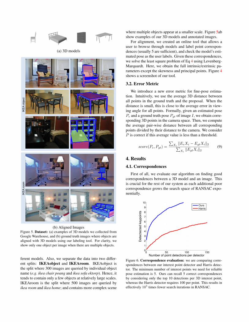
(a) 3D models

IKE

A ob

ject

IK

EA

room

(b) Aligned ImagesFigure 5. Dataset: (a) examples of 3D models we collected fromGoogle Warehouse, and (b) ground truth images where objects arealigned with 3D models using our labeling tool. For clarity, weshow only one object per image when there are multiple objects.

ferent models. Also, we separate the data into two differ-ent splits: IKEAobject and IKEAroom. IKEAobject isthe split where 300 images are queried by individual objectname (e.g. ikea chair poang and ikea sofa ektorp). Hence, ittends to contain only a few objects at relatively large scales.IKEAroom is the split where 500 images are queried byikea room and ikea home; and contains more complex scene

where multiple objects appear at a smaller scale. Figure 5abshow examples of our 3D models and annotated images.

For alignment, we created an online tool that allows auser to browse through models and label point correspon-dences (usually 5 are sufficient), and check the model’s esti-mated pose as the user labels. Given these correspondences,we solve the least square problem of Eq 4 using Levenberg-Marquardt. Here, we obtain the full intrinsic/extrinsic pa-rameters except the skewness and principal points. Figure 4shows a screenshot of our tool.

3.2. Error MetricWe introduce a new error metric for fine-pose estima-

tion. Intuitively, we use the average 3D distance betweenall points in the ground truth and the proposal. When thedistance is small, this is close to the average error in view-ing angle for all points. Formally, given an estimated posePe and a ground truth pose Pgt of image I , we obtain corre-sponding 3D points in the camera space. Then, we computethe average pair-wise distance between all correspondingpoints divided by their distance to the camera. We considerP is correct if this average value is less than a threshold.

score(Pe, Pgt) =

PXi

kEeXi � EgtXik2PXi

kEgtXik2(9)

4. Results4.1. Correspondences

First of all, we evaluate our algorithm on finding goodcorrespondences between a 3D model and an image. Thisis crucial for the rest of our system as each additional poorcorrespondence grows the search space of RANSAC expo-nentially.

0 50 100 1500

1

2

3

4

5

6

7

8

9

10

Number of point detections per detector

Dete

ctect

ed k

eyp

oin

ts

OursHarris

Figure 6. Correspondence evaluation: we are comparing corre-spondences between our interest point detector and Harris detec-tor. The minimum number of interest points we need for reliablepose estimation is 5. Ours can recall 5 correct correspondencesby considering only the top 10 detections per 3D interest point,whereas the Harris detector requires 100 per point. This results ineffectively 105 times fewer search iterations in RANSAC.

Figure 6 shows our evaluation. We compare Harris cor-ner detectors against our detector based on LDA classifiers.On average, to capture 5 correct correspondences with ourmethod, each interest point has to consider only its top 10matched candidates. In contrast, using the Harris corner de-tector, one needs to consider about 100 candidates. Thishelps finding good candidates in the RANSAC algorithm.

4.2. Initial Poses

101

102

103

0

0.1

0.2

0.3

0.4

0.5

0.6

0.7

0.8

0.9

1

Candidates per Image

Re

call

Figure 7. RANSAC evaluation: we evaluated how many posecandidates per image we need in order to obtain a certain recall.We need only about 2000 candidates in order to have 0.9 recall.This allows us to perform a computationally expensive feature ex-traction on only a small number of candidates.

In order for us to find the pose P minimizing S(P, c),we need to ensure that our set of poses {(P, c)} minimiz-ing L(P, c) + D(P, c) contains at least one correct pose.The recall of our full model is upper bonded by that of thisset. Figure 7 shows a semi-log plot of recall vs minimumnumber of top candidates required per image. Consideringthe top 2000 candidate poses (shown with a red line) fromRANSAC, we can obtain 0.9 recall. In other words, thelater optimization, where feature extraction is computation-ally heavy, can run with only the top 2000 candidate posesand still have a recall 0.9.

4.3. Final Pose EstimationTable 1 shows the evaluation of our method with various

sets of features as well as two state-of-the-art object detec-tors: Deformable part models [4] and Exemplar LDA [8] inIKEAobject database.

For both [4] and [8], we trained detectors using the codeprovided by the authors. The training set contains renderedimages (examples are shown in Figure 5b) in order to covervarious poses (which are not possible to cover with real im-ages). Note the low performances of [4] and [8]. We believethere are two major issues: (1) they are trained with a verylarge number of mixtures. If there are some mixtures with

high false positive rates, then the whole system can breakdown, and (2) they are trained with rendered images due totheir requirement of images for each different mixture. Hav-ing a different modality can result in a poor performance.

Our average precision (AP) is computed based on ourerror metric (Eq. 9). We score each pose estimation P asa true detection if its normalized 3D space distance to theground truth is within the threshold; and for the rest, we pre-cisely follow a standard bounding box criterion [2]. Here,we would like to emphasize that this is a much harder taskthan a typical bounding box detection task. Hence, low APin the range of 0-0.02 should not be misleading.

D + L, based on RANSAC, has a low performance byitself. Though it is true that the top candidates generallycontain a correct pose (as shown in Figure 7), it is clear thatscores based only on local correspondences (D and L) arenot robust to false positives, despite high recall.

We also evaluated two other features based on HOG andRegion features. Adding these two features greatly boostsperformance. HOG and Region features were added forcapturing global shape similarity. Our full method takesabout 12 minutes on a single core for each image and model.

Figure 8. Corner cases: these two images illustrate cases whichare incorrect under our pose estimation criteria, but are still correctunder standard bounding box detection criterion.

Also, we compared our method against [4, 8] on a detec-tion task as shown in Table 2. For our method, we ran thesame full pipeline and extracted bounding boxes from theestimated poses. For the detection task, we trained [4, 8]with real images, because there exist enough real images totrain a small number of mixtures. We train/test on 10 dif-ferent random splits. Because our method is designed forcapturing a fine alignment, we measured at two differentthresholds on bounding box intersection over union. One isthe standard threshold of 0.5 and the other one is a higherthreshold of 0.8. As the table shows, our method does notfluctuate much with a threshold change, whereas both [8]and [4] suffer and drop performances significantly. Figure8 shows several detection examples where pose estimationis incorrect, but still bounding box estimation is correct witha threshold of 0.5.

Lastly, Figure 9 shows our qualitative results. We firstshow our pose predictions by drawing blue outlines, andpredicted normal directions. To show that our algorithm ob-tained an accurate pose alignment, we also render different

(a) Image (b) Our result (c) Normal map (d) Novel view

Figure 9. Final results: we show qualitative results of our method. (b) shows our estimated pose, (c) shows a normal direction, and (d)shows a synthesized novel view by rotating along y-axis. First 4 rows are correct estimations and last 2 rows are incorrect. Note that anerror on the 5th row is misaligning a bookcase by 1 shelf. Near symmetry and repetition cause this type of top false positives.

chair bookcase sofa table bed bookcase desk bookcase bed bookcase stoolpoang billy1 ektorp lack malm1 billy2 expedit billy3 malm2 billy4 poang mean

DPM 0.02 0.27 0.08 0.22 0.24 0.35 0.09 0.18 0.66 0.11 0.76 0.27ELDA 0.29 0.24 0.35 0.14 0.06 0.77 0.03 0.20 0.60 0.41 0.13 0.29D+L 0.045 0.014 0.071 0.011 0.007 0.069 0.008 0.587 0.038 0.264 0.003 0.10

D+L+HOG 4.48 2.91 0.17 5.56 0.64 9.70 0.12 5.05 15.39 7.72 0.79 4.78D+L+H+Region 17.16 11.35 2.43 7.24 2.37 17.18 1.23 7.70 14.24 9.08 3.42 8.49

Full 18.76 15.77 4.43 11.27 6.12 20.62 6.87 7.71 14.56 15.09 7.20 11.67Table 1. AP Performances on Pose Estimation: we evaluate our pose estimation performance at a fine scale in the IKEAobject database.As we introduce more features, the performance significantly improves. Note that DPM and ELDA are trained using rendered images.

chair bookcase sofa table bed bookcase desk bookcase bed bookcase stoolpoang billy1 ektorp lack malm1 billy2 expedit billy3 malm2 billy4 poang mean

LDA @ 0.5 15.02 5.22 8.91 1.59 15.46 3.08 37.62 34.52 1.85 46.92 0.37 15.51DPM @ 0.5 27.46 24.28 12.14 10.75 3.41 13.54 46.13 34.22 0.95 0.12 0.53 15.78Ours @ 0.5 23.17 24.21 6.27 13.93 27.12 26.33 18.42 23.84 22.34 32.19 8.16 20.54LDA @ 0.8 4.71 0.62 7.49 1.24 3.52 0.11 18.76 21.73 1.27 7.09 0.17 6.06DPM @ 0.8 7.78 0.56 10.13 0.01 1.25 0.00 35.03 12.73 0.00 0.00 0.44 6.18Ours @ 0.8 21.74 18.55 5.24 11.93 11.42 25.87 8.99 10.24 18.14 17.92 7.38 14.31

Table 2. AP Performances on Detection: we evaluate our method on detection against [4] and [8] at two different bounding boxintersection over union thresholds (0.5 and 0.8) in the IKEAobject database. The gap between our method and [4] becomes significantlylarger as we increase the threshold; which suggests that our method is better at fine detection.

novel views with a simple texture mapping.

5. ConclusionWe have introduced a novel problem and model of

estimating fine-pose of objects in the image with exact3D models, combining traditionally used and recentlydeveloped techniques. Moreover, we also provide a newdataset of images fine-aligned with exactly matched 3Dmodels, as well as a set of 3D models for widely usedobjects. We believe our approach can extend further tomore generic object classes, and enable the community totry more ambitious goals such as accurate 3D contextualmodeling and full 3D room parsing.

Acknowledgements: This work is funded by ONRMURI N000141010933. We also thank Phillip Isola andAditya Khosla for important suggestions and discussion.

References[1] N. Dalal and B. Triggs. Histograms of oriented gradients for human

detection. In CVPR, 2005. 2[2] M. Everingham, L. Van Gool, C. K. I. Williams, J. Winn, and

A. Zisserman. The PASCAL Visual Object Classes Challenge 2007(VOC2007) Results. 6

[3] P. Felzenszwalb and D. Huttenlocher. Efficient graph-based imagesegmentation. IJCV, 59(2):167–181, 2004. 3

[4] P. F. Felzenszwalb, R. B. Girshick, and D. McAllester. Discrimina-tively trained deformable part models, release 4. 6, 8

[5] S. Fidler, S. J. Dickinson, and R. Urtasun. 3d object detection andviewpoint estimation with a deformable 3d cuboid model. In NIPS,2012. 2

[6] M. Fisher and P. Hanrahan. Context-based search for 3d models.ACM Trans. Graph., 29(6), Dec. 2010. 2

[7] S. Gupta, P. Arbelaez, and J. Malik. Perceptual organization andrecognition of indoor scenes from RGB-D images. In CVPR, 2013.2

[8] B. Hariharan, J. Malik, and D. Ramanan. Discriminative decorrela-tion for clustering and classification. In ECCV, 2012. 3, 6, 8

[9] M. Hejrati and D. Ramanan. Analyzing 3d objects in cluttered im-ages. In NIPS, 2012. 2

[10] P. Henry, M. Krainin, E. Herbst, X. Ren, and D. Fox. Rgbd mapping:Using depth cameras for dense 3d modeling of indoor environments.In RGB-D: Advanced Reasoning with Depth Cameras Workshop inconjunction with RSS, 2010. 2

[11] J. J. Lim, C. L. Zitnick, and P. Dollar. Sketch tokens: A learnedmid-level representation for contour and object detection. In CVPR,2013. 4

[12] D. Lowe. Fitting parameterized three-dimensional models to images.PAMI, 1991. 1, 3

[13] D. G. Lowe. Distinctive image features from scale-invariant key-points. IJCV, 2004. 2

[14] J. L. Mundy. Object recognition in the geometric era: A retrospec-tive. In Toward CategoryLevel Object Recognition, volume 4170 ofLecture Notes in Computer Science, pages 3–29. Springer, 2006. 1

[15] T. Ojala, M. Pietikinen, and T. Menp. Multiresolution gray-scaleand rotation invariant texture classification with local binary patterns.PAMI, 2002. 4

[16] B. Pepik, P. Gehler, M. Stark, and B. Schiele. 3d2pm - 3d deformablepart models. In ECCV, 2012. 2

[17] F. Rothganger, S. Lazebnik, C. Schmid, and J. Ponce. 3d object mod-eling and recognition using local affine-invariant image descriptorsand multi-view spatial constraints. IJCV, 66:2006, 2006. 1

[18] S. Satkin, J. Lin, and M. Hebert. Data-driven scene understandingfrom 3D models. In BMVC, 2012. 4

[19] Y. Xiang and S. Savarese. Estimating the aspect layout of objectcategories. In CVPR, 2012. 2

[20] J. Xiao, B. Russell, and A. Torralba. Localizing 3d cuboids in single-view images. In NIPS. 2012. 2, 4

[21] Y. Zhao and S.-C. Zhu. Image parsing via stochastic scene grammar.In NIPS, 2011. 2