Parfor for MATLAB - People - Department of Scientific …jburkardt/presentations/... · ·...
101
Parfor for MATLAB Summer Seminar ISC5939 .......... John Burkardt Department of Scientific Computing Florida State University http://people.sc.fsu.edu/∼jburkardt/presentations/. . . . . . parfor 2012 fsu.pdf 24/26 July 2012 1 / 101
Transcript of Parfor for MATLAB - People - Department of Scientific …jburkardt/presentations/... · ·...
Parfor for MATLAB
Summer SeminarISC5939..........
John BurkardtDepartment of Scientific Computing
Florida State Universityhttp://people.sc.fsu.edu/∼jburkardt/presentations/. . .
. . . parfor 2012 fsu.pdf
24/26 July 2012
1 / 101
MATLAB Parallel Computing
Introduction
QUAD Example (PARFOR)
MD Example
PRIME Example
ODE Example
SPMD: Single Program, Multiple Data
QUAD Example (SPMD)
DISTANCE Example
CONTRAST Example
CONTRAST2: Messages
Conclusion
2 / 101

INTRO: Parallel MATLAB on Your Desktop
Parallel MATLAB is an extension of MATLAB that takes advantage ofmulticore desktop machines and clusters.
The Parallel Computing Toolbox or PCT runs on a desktop, and cantake advantage of up to 12 cores there.
The user can:
type in commands that will be executed in parallel, OR
call an M-file that will run in parallel, OR
submit an M-file to be executed in “batch” (not interactively).
3 / 101
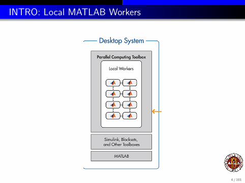
INTRO: Local MATLAB Workers
4 / 101
INTRO: Parallel MATLAB on a Cluster
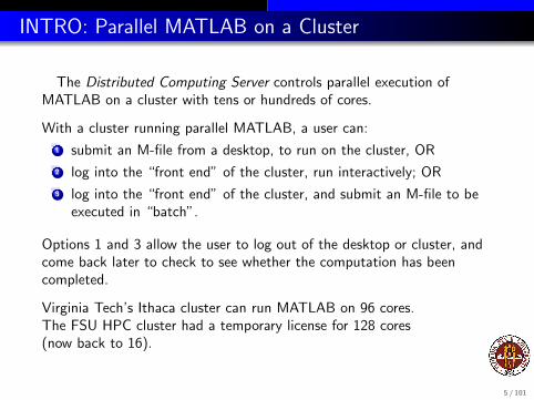
The Distributed Computing Server controls parallel execution ofMATLAB on a cluster with tens or hundreds of cores.
With a cluster running parallel MATLAB, a user can:
1 submit an M-file from a desktop, to run on the cluster, OR
2 log into the “front end” of the cluster, run interactively; OR
3 log into the “front end” of the cluster, and submit an M-file to beexecuted in “batch”.
Options 1 and 3 allow the user to log out of the desktop or cluster, andcome back later to check to see whether the computation has beencompleted.
Virginia Tech’s Ithaca cluster can run MATLAB on 96 cores.The FSU HPC cluster had a temporary license for 128 cores(now back to 16).
5 / 101

INTRO: Local and Remote MATLAB Workers
6 / 101

INTRO: PARFOR and SPMD (and TASK)
There are several ways to write a parallel MATLAB program:
some for loops can be made into parallel parfor loops;
the spmd statement synchronizes cooperating processors;
the task statement submits a program many times with differentinput, as in a Monte Carlo calculation; all the outputs can beanalyzed together at the end.
parfor is a way to run FOR loops in parallel, similar to OpenMP.
spmd allows you to design almost any kind of parallel computation; it ispowerful, but requires rethinking the program and data. It is similar toMPI.
We won’t have time to talk about the task statement.
7 / 101
INTRO: Execution
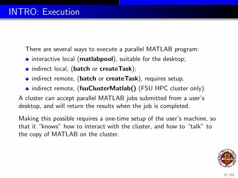
There are several ways to execute a parallel MATLAB program:
interactive local (matlabpool), suitable for the desktop;
indirect local, (batch or createTask);
indirect remote, (batch or createTask), requires setup.
indirect remote, (fsuClusterMatlab() (FSU HPC cluster only).
A cluster can accept parallel MATLAB jobs submitted from a user’sdesktop, and will return the results when the job is completed.
Making this possible requires a one-time setup of the user’s machine, sothat it “knows” how to interact with the cluster, and how to “talk” tothe copy of MATLAB on the cluster.
8 / 101
MATLAB Parallel Computing
Introduction
QUAD Example (PARFOR)
MD Example
PRIME Example
ODE Example
SPMD: Single Program, Multiple Data
QUAD Example (SPMD)
DISTANCE Example
CONTRAST Example
CONTRAST2: Messages
Conclusion
9 / 101
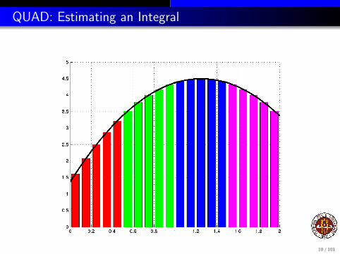
QUAD: Estimating an Integral
10 / 101

QUAD: The QUAD FUN Function
function q = quad_fun ( n, a, b )
q = 0.0;w = ( b - a ) / n;
for i = 1 : nx = ( ( n - i ) * a + ( i - 1 ) * b ) / ( n - 1 );fx = bessely ( 4.5, x );q = q + w * fx;
end
returnend
11 / 101

QUAD: Comments
The function quad fun estimates the integral of a particular functionover the interval [a, b].
It does this by evaluating the function at n evenly spaced points,multiplying each value by the weight (b − a)/n.
These quantities can be regarded as the areas of little rectangles that lieunder the curve, and their sum is an estimate for the total area under thecurve from a to b.
We could compute these subareas in any order we want.
We could even compute the subareas at the same time, assuming there issome method to save the partial results and add them together in anorganized way.
12 / 101

QUAD: The Parallel QUAD FUN Function
function q = quad_fun ( n, a, b )
q = 0.0;w = ( b - a ) / n;
parfor i = 1 : nx = ( ( n - i ) * a + ( i - 1 ) * b ) / ( n - 1 );fx = bessely ( 4.5, x );q = q + w * fx;
end
returnend
http://people.sc.fsu.edu/∼jburkardt/m src/quad parfor/quad parfor.html
13 / 101
QUAD: Comments
The parallel version of quad fun does the same calculations.
The parfor statement changes how this program does the calculations. Itasserts that all the iterations of the loop are independent, and can bedone in any order, or in parallel.
Execution begins with a single processor, the client. When a parfor loopis encountered, the client is helped by a “pool” of workers.
Each worker is assigned some iterations of the loop. Once the loop iscompleted, the client resumes control of the execution.
MATLAB ensures that the results are the same whether the program isexecuted sequentially, or with the help of workers.
The user can wait until execution time to specify how many workers areactually available.
14 / 101
QUAD: What Do You Need For Parallel MATLAB?
1 Your machine should have multiple processors or cores:
On a PC: Start :: Settings :: Control Panel :: SystemOn a Mac: Apple Menu :: About this Mac :: More Info...On Linux: System Menu :: About this Computer
2 Your MATLAB must be version 2008a or later:
Go to the HELP menu, and choose About Matlab.
3 You must have the Parallel Computing Toolbox (PCT):
To list all your toolboxes, type the MATLAB command ver.
Machines in DSL 400B have 2 processors; machines in DSL 152 have 8.They all have a recent copy of MATLAB with the PCT.
15 / 101
QUAD: Interactive Execution with MATLABPOOL
Workers are gathered using the matlabpool command.
To run quad fun.m in parallel on your desktop, type:
n = 10000; a = 0; b = 1;matlabpool open local 4q = quad_fun ( n, a, b );matlabpool close
The word local is choosing the local configuration, that is, the coresassigned to be workers will be on the local machine.
The value ”4” is the number of workers you are asking for. It can be upto 12 on a local machine. It does not have to match the number of coresyou have.
16 / 101
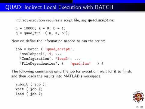
QUAD: Indirect Local Execution with BATCH
Indirect execution requires a script file, say quad script.m:
n = 10000; a = 0; b = 1;q = quad_fun ( n, a, b );
Now we define the information needed to run the script:
job = batch ( ’quad_script’,’matlabpool’, 4, ...’Configuration’, ’local’, ...’FileDependencies’, { ’quad_fun’ } )
The following commands send the job for execution, wait for it to finish,and then loads the results into MATLAB’s workspace:
submit ( job );wait ( job );load ( job );
17 / 101

QUAD: Indirect Remote Execution with BATCH
The batch command can send your job anywhere, and get the resultsback, if you have set up an account on the remote machine, and havedefined a configuration on your desktop that describes how to access theremote machine.
For example, at Virginia Tech, a desktop computer can send a batch jobto the cluster, requesting 32 cores:
job = batch ( ’quad_script’, ...’matlabpool’, 32, ...’Configuration’, ’ithaca_2011b’, ...’FileDependencies’, { ’quad_fun’ } )
You submit the job, wait for it, and load the data the same way as for alocal batch job.
18 / 101

MATLAB Parallel Computing
Introduction
QUAD Example (PARFOR)
MD Example
PRIME Example
ODE Example
SPMD: Single Program, Multiple Data
QUAD Example (SPMD)
DISTANCE Example
CONTRAST Example
CONTRAST2: Messages
Conclusion
19 / 101
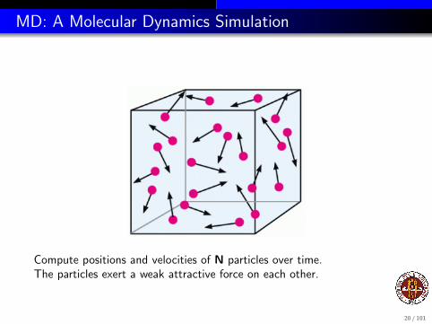
MD: A Molecular Dynamics Simulation
Compute positions and velocities of N particles over time.The particles exert a weak attractive force on each other.
20 / 101

MD: The Molecular Dynamics Example
How do you prepare a program to run in parallel?
The MD program runs a simple molecular dynamics simulation.
There are N molecules being simulated.
The program runs a long time; a parallel version would run faster.
There are many for loops in the program that we might replace byparfor, but it is a mistake to try to parallelize everything!
MATLAB has a profile command that can report where the CPU timewas spent - which is where we should try to parallelize.
21 / 101
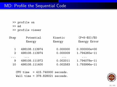
MD: Profile the Sequential Code
>> profile on>> md>> profile viewer
Step Potential Kinetic (P+K-E0)/E0Energy Energy Energy Error
1 498108.113974 0.000000 0.000000e+002 498108.113974 0.000009 1.794265e-11
... ... ... ...9 498108.111972 0.002011 1.794078e-1110 498108.111400 0.002583 1.793996e-11
CPU time = 415.740000 seconds.Wall time = 378.828021 seconds.
22 / 101
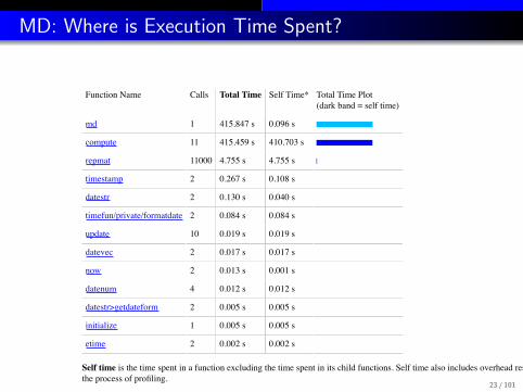
MD: Where is Execution Time Spent?This is a static copy of a profile report
Home
Profile SummaryGenerated 27-Apr-2009 15:37:30 using cpu time.
Function Name Calls Total Time Self Time* Total Time Plot
(dark band = self time)
md 1 415.847 s 0.096 s
compute 11 415.459 s 410.703 s
repmat 11000 4.755 s 4.755 s
timestamp 2 0.267 s 0.108 s
datestr 2 0.130 s 0.040 s
timefun/private/formatdate 2 0.084 s 0.084 s
update 10 0.019 s 0.019 s
datevec 2 0.017 s 0.017 s
now 2 0.013 s 0.001 s
datenum 4 0.012 s 0.012 s
datestr>getdateform 2 0.005 s 0.005 s
initialize 1 0.005 s 0.005 s
etime 2 0.002 s 0.002 s
Self time is the time spent in a function excluding the time spent in its child functions. Self time also includes overhead resulting from
the process of profiling.
Profile Summary file://localhost/Users/burkardt/public_html/m_src/md/md_profile.txt/file0.html
1 of 1 4/27/09 3:39 PM
23 / 101
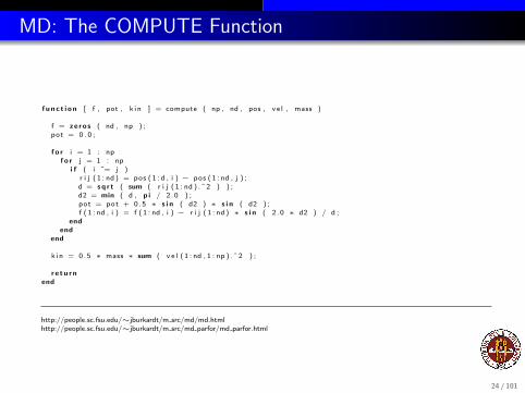
MD: The COMPUTE Function
f u n c t i o n [ f , pot , k i n ] = compute ( np , nd , pos , v e l , mass )
f = z e r o s ( nd , np ) ;pot = 0 . 0 ;
f o r i = 1 : npf o r j = 1 : np
i f ( i ˜= j )r i j ( 1 : nd ) = pos ( 1 : d , i ) − pos ( 1 : nd , j ) ;d = s q r t ( sum ( r i j ( 1 : nd ) . ˆ 2 ) ) ;d2 = min ( d , p i / 2 .0 ) ;pot = pot + 0 .5 ∗ s i n ( d2 ) ∗ s i n ( d2 ) ;f ( 1 : nd , i ) = f ( 1 : nd , i ) − r i j ( 1 : nd ) ∗ s i n ( 2 . 0 ∗ d2 ) / d ;
endend
end
k i n = 0 .5 ∗ mass ∗ sum ( v e l ( 1 : nd , 1 : np ) . ˆ 2 ) ;
r e t u r nend
http://people.sc.fsu.edu/∼jburkardt/m src/md/md.htmlhttp://people.sc.fsu.edu/∼jburkardt/m src/md parfor/md parfor.html
24 / 101

MD: Can We Use PARFOR?
The compute function fills the force vector f(i) using a for loop.
Iteration i computes the force on particle i, determining the distance toeach particle j, squaring, truncating, taking the sine.
The computation for each particle is “independent”; nothing computed inone iteration is needed by, nor affects, the computation in anotheriteration. We could compute each value on a separate worker, at thesame time.
The MATLAB command parfor will distribute the iterations of this loopacross the available workers.
Tricky question: Could we parallelize the j loop instead?
Tricky question: Could we parallelize both loops?
25 / 101

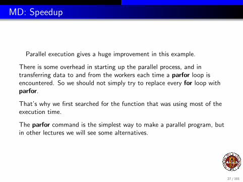
MD: Speedup
Replacing “for i” by “parfor i”, here is our speedup:
26 / 101
MD: Speedup
Parallel execution gives a huge improvement in this example.
There is some overhead in starting up the parallel process, and intransferring data to and from the workers each time a parfor loop isencountered. So we should not simply try to replace every for loop withparfor.
That’s why we first searched for the function that was using most of theexecution time.
The parfor command is the simplest way to make a parallel program, butin other lectures we will see some alternatives.
27 / 101

MD: PARFOR is Particular
We were only able to parallelize the loop because the iterations wereindependent, that is, the results did not depend on the order in which theiterations were carried out.
In fact, to use MATLAB’s parfor in this case requires some extraconditions, which are discussed in the PCT User’s Guide. Briefly, parforis usable when vectors and arrays that are modified in the calculation canbe divided up into distinct slices, so that each slice is only needed for oneiteration.
This is a stronger requirement than independence of order!
Trick question: Why was the scalar value POT acceptable?
28 / 101
MATLAB Parallel Computing
Introduction
QUAD Example (PARFOR)
MD Example
PRIME Example
ODE Example
SPMD: Single Program, Multiple Data
QUAD Example (SPMD)
DISTANCE Example
CONTRAST Example
CONTRAST2: Messages
Conclusion
29 / 101
PRIME: The Prime Number Example
For our next example, we want a simple computation involving a loopwhich we can set up to run for a long time.
We’ll choose a program that determines how many prime numbers thereare between 1 and N.
If we want the program to run longer, we increase the variable N.Doubling N multiplies the run time roughly by 4.
30 / 101
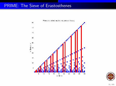
PRIME: The Sieve of Erastosthenes
31 / 101
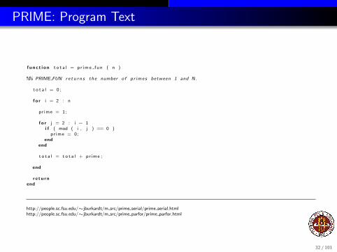
PRIME: Program Text
f u n c t i o n t o t a l = p r ime fun ( n )
%% PRIME FUN r e t u r n s the number o f p r imes between 1 and N.
t o t a l = 0 ;
f o r i = 2 : n
pr ime = 1 ;
f o r j = 2 : i − 1i f ( mod ( i , j ) == 0 )
pr ime = 0 ;end
end
t o t a l = t o t a l + pr ime ;
end
r e t u r nend
http://people.sc.fsu.edu/∼jburkardt/m src/prime serial/prime serial.htmlhttp://people.sc.fsu.edu/∼jburkardt/m src/prime parfor/prime parfor.html
32 / 101

PRIME: We can run this in parallel
We can parallelize the loop whose index is i, replacing for by parfor.The computations for different values of i are independent.
There is one variable that is not independent of the loops, namely total.This is simply computing a running sum (a reduction variable), and weonly care about the final result. MATLAB is smart enough to be able tohandle this summation in parallel.
To make the program parallel, we replace for by parfor. That’s all!
33 / 101
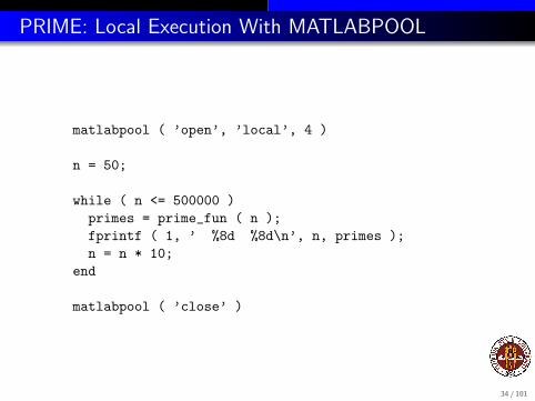
PRIME: Local Execution With MATLABPOOL
matlabpool ( ’open’, ’local’, 4 )
n = 50;
while ( n <= 500000 )primes = prime_fun ( n );fprintf ( 1, ’ %8d %8d\n’, n, primes );n = n * 10;
end
matlabpool ( ’close’ )
34 / 101

PRIME: Timing
PRIME_PARFOR_RUNRun PRIME_PARFOR with 0, 1, 2, and 4 workers.Time is measured in seconds.
N 1+0 1+1 1+2 1+4
50 0.067 0.179 0.176 0.278500 0.008 0.023 0.027 0.0325000 0.100 0.142 0.097 0.06150000 7.694 9.811 5.351 2.719
500000 609.764 826.534 432.233 222.284
35 / 101

PRIME: Timing Comments
There are many thoughts that come to mind from these results!
Why does 500 take less time than 50? (It doesn’t, really).
How can ”1+1” take longer than ”1+0”?(It does, but it’s probably not as bad as it looks!)
This data suggests two conclusions:
Parallelism doesn’t pay until your problem is big enough;
AND
Parallelism doesn’t pay until you have a decent number of workers.
36 / 101

MATLAB Parallel Computing
Introduction
QUAD Example (PARFOR)
MD Example
PRIME Example
ODE Example
SPMD: Single Program, Multiple Data
QUAD Example (SPMD)
DISTANCE Example
CONTRAST Example
CONTRAST2: Messages
Conclusion
37 / 101
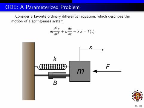
ODE: A Parameterized Problem
Consider a favorite ordinary differential equation, which describes themotion of a spring-mass system:
md2x
dt2+ b
dx
dt+ k x = f (t)
38 / 101

ODE: A Parameterized Problem
Solutions of this equation describe oscillatory behavior; x(t) swingsback and forth, in a pattern determined by the parameters m, b, k, f andthe initial conditions.
Each choice of parameters defines a solution, and let us suppose that thequantity of interest is the maximum deflection xmax that occurs for eachsolution.
We may wish to investigate the influence of b and k on this quantity,leaving m fixed and f zero.
So our computation might involve creating a plot of xmax(b, k).
39 / 101

ODE: Each Solution has a Maximum Value
40 / 101
ODE: A Parameterized Problem
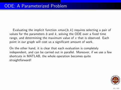
Evaluating the implicit function xmax(b, k) requires selecting a pair ofvalues for the parameters b and k , solving the ODE over a fixed timerange, and determining the maximum value of x that is observed. Eachpoint in our graph will cost us a significant amount of work.
On the other hand, it is clear that each evaluation is completelyindependent, and can be carried out in parallel. Moreover, if we use a fewshortcuts in MATLAB, the whole operation becomes quitestraightforward!
41 / 101
ODE: The Function
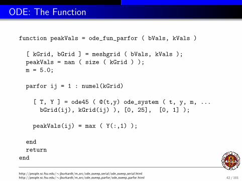
function peakVals = ode_fun_parfor ( bVals, kVals )
[ kGrid, bGrid ] = meshgrid ( bVals, kVals );peakVals = nan ( size ( kGrid ) );m = 5.0;
parfor ij = 1 : numel(kGrid)
[ T, Y ] = ode45 ( @(t,y) ode_system ( t, y, m, ...bGrid(ij), kGrid(ij) ), [0, 25], [0, 1] );
peakVals(ij) = max ( Y(:,1) );
endreturn
end
http://people.sc.fsu.edu/∼jburkardt/m src/ode sweep serial/ode sweep serial.htmlhttp://people.sc.fsu.edu/∼jburkardt/m src/ode sweep parfor/ode sweep parfor.html 42 / 101

ODE: The Script
If we want to use the batch (indirect or remote execution) option, thenwe need to call the function using a script. We’ll call this“ode script batch.m”
bVals = 0.1 : 0.05 : 5;kVals = 1.5 : 0.05 : 5;
peakVals = ode_fun_parfor ( bVals, kVals );
43 / 101

ODE: Plot the Results
The script ode display.m calls surf for a 3D plot.
Our parameter arrays bVals and kVals are X and Y, while the computedarray peakVals plays the role of Z.
figure;
surf ( bVals, kVals, peakVals, ...’EdgeColor’, ’Interp’, ’FaceColor’, ’Interp’ );
title ( ’Results of ODE Parameter Sweep’ )xlabel ( ’Damping B’ );ylabel ( ’Stiffness K’ );zlabel ( ’Peak Displacement’ );view ( 50, 30 )
44 / 101

ODE: Interactive Execution
Using the interactive option, we set up the input, get the workers, andcall the function:
bVals = 0.1 : 0.05 : 5;kVals = 1.5 : 0.05 : 5;
matlabpool open local 4
peakVals = ode_fun_parfor ( bVals, kVals );
matlabpool close
ode_display <-- Don’t need parallel option here.
45 / 101
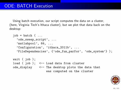
ODE: BATCH Execution
Using batch execution, our script computes the data on a cluster,(here, Virginia Tech’s Ithaca cluster), but we plot that data back on thedesktop:
job = batch ( ...’ode_sweep_script’, ...’matlabpool’, 64, ...’Configuration’, ’ithaca_2011b’, ...’FileDependencies’, {’ode_fun_parfor’, ’ode_system’} );
wait ( job );load ( job ); <-- Load data from clusterode_display <-- The desktop plots the data that
was computed on the cluster
46 / 101

ODE: A Parameterized Problem
47 / 101
MATLAB Parallel Computing - End of Part 1
48 / 101

MATLAB Parallel Computing
Introduction
QUAD Example (PARFOR)
MD Example
PRIME Example
ODE Example
SPMD: Single Program, Multiple Data
QUAD Example (SPMD)
DISTANCE Example
CONTRAST Example
CONTRAST2: Messages
Conclusion
49 / 101

SPMD: Single Program, Multiple Data
The SPMD command is like a very simplified version of MPI. There isone client process, supervising workers who cooperate on a singleprogram. Each worker (sometimes also called a “lab”) has an identifier,knows how many workers there are total, and can determine its behaviorbased on that ID.
each worker runs on a separate core (ideally);
each worker uses separate workspace;
a common program is used;
workers meet at synchronization points;
the client program can examine or modify data on any worker;
any two workers can communicate directly via messages.
50 / 101
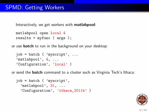
SPMD: Getting Workers
Interactively, we get workers with matlabpool:
matlabpool open local 4results = myfunc ( args );
or use batch to run in the background on your desktop:
job = batch ( ’myscript’, ...’matlabpool’, 4, ...’Configuration’, ’local’ )
or send the batch command to a cluster such as Virginia Tech’s Ithaca:
job = batch ( ’myscript’,’matlabpool’, 31, ...’Configuration’, ’ithaca_2011b’ )
51 / 101
SPMD: The SPMD Environment
MATLAB sets up one special worker called the client.
MATLAB sets up the requested number of workers, each with a copy ofthe program. Each worker “knows” it’s a worker, and has access to twospecial functions:
numlabs(), the number of workers;
labindex(), a unique identifier between 1 and numlabs().
The empty parentheses are usually dropped, but remember, these arefunctions, not variables!
If the client calls these functions, they both return the value 1! That’sbecause when the client is running, the workers are not. The client coulddetermine the number of workers available by
n = matlabpool ( ’size’ )
52 / 101
SPMD: The SPMD Command
The client and the workers share a single program in which somecommands are delimited within blocks opening with spmd and closingwith end.
The client executes commands up to the first spmd block, when itpauses. The workers execute the code in the block. Once they finish, theclient resumes execution.
The client and each worker have separate workspaces, but it is possiblefor them to communicate and trade information.
The value of variables defined in the “client program” can be referencedby the workers, but not changed.
Variables defined by the workers can be referenced or changedby the client, but a special syntax is used to do this.
53 / 101
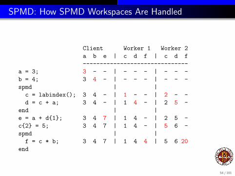
SPMD: How SPMD Workspaces Are Handled
Client Worker 1 Worker 2a b e | c d f | c d f-------------------------------
a = 3; 3 - - | - - - | - - -b = 4; 3 4 - | - - - | - - -spmd | |c = labindex(); 3 4 - | 1 - - | 2 - -d = c + a; 3 4 - | 1 4 - | 2 5 -
end | |e = a + d{1}; 3 4 7 | 1 4 - | 2 5 -c{2} = 5; 3 4 7 | 1 4 - | 5 6 -spmd | |f = c * b; 3 4 7 | 1 4 4 | 5 6 20
end
54 / 101
SPMD: When is Workspace Preserved?
A program can contain several spmd blocks. When execution of oneblock is completed, the workers pause, but they do not disappear andtheir workspace remains intact. A variable set in one spmd block will stillhave that value if another spmd block is encountered.
You can imagine the client and workers simply alternate execution.
In MATLAB, variables defined in a function “disappear” once thefunction is exited. The same thing is true, in the same way, for aMATLAB program that calls a function containing spmd blocks. Whileinside the function, worker data is preserved from one block to another,but when the function is completed, the worker data defined theredisappears, just as regular MATLAB data does.
55 / 101
MATLAB Parallel Computing
Introduction
QUAD Example (PARFOR)
MD Example
PRIME Example
ODE Example
SPMD: Single Program, Multiple Data
QUAD Example (SPMD)
DISTANCE Example
CONTRAST Example
CONTRAST2: Messages
Conclusion
56 / 101

QUAD SPMD: The Trapezoid Rule
Area of one trapezoid = average height * base.
57 / 101
QUAD SPMD: The Trapezoid Rule
To estimate the area under a curve using one trapezoid, we write∫ b
a
f (x) dx ≈ (1
2f (a) +
1
2f (b)) ∗ (b − a)
We can improve this estimate by using n − 1 trapezoids defined byequally spaced points x1 through xn:∫ b
a
f (x) dx ≈ (1
2f (x1) + f (x2) + ... + f (xn−1) +
1
2f (xn)) ∗ b − a
n − 1
If we have several workers available, then each one can get a part of theinterval to work on, and compute a trapezoid estimate there. By addingthe estimates, we get an approximate to the integral of the function overthe whole interval.
58 / 101
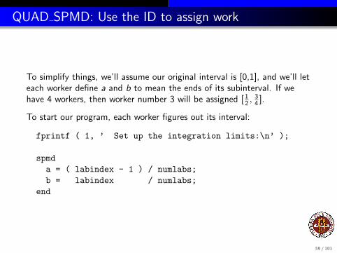
QUAD SPMD: Use the ID to assign work
To simplify things, we’ll assume our original interval is [0,1], and we’ll leteach worker define a and b to mean the ends of its subinterval. If wehave 4 workers, then worker number 3 will be assigned [ 1
2 , 34 ].
To start our program, each worker figures out its interval:
fprintf ( 1, ’ Set up the integration limits:\n’ );
spmda = ( labindex - 1 ) / numlabs;b = labindex / numlabs;
end
59 / 101
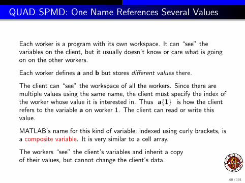
QUAD SPMD: One Name References Several Values
Each worker is a program with its own workspace. It can “see” thevariables on the client, but it usually doesn’t know or care what is goingon on the other workers.
Each worker defines a and b but stores different values there.
The client can “see” the workspace of all the workers. Since there aremultiple values using the same name, the client must specify the index ofthe worker whose value it is interested in. Thus a{1} is how the clientrefers to the variable a on worker 1. The client can read or write thisvalue.
MATLAB’s name for this kind of variable, indexed using curly brackets, isa composite variable. It is very similar to a cell array.
The workers “see” the client’s variables and inherit a copyof their values, but cannot change the client’s data.
60 / 101
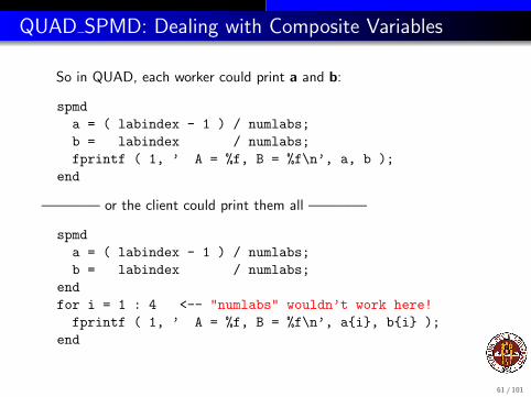
QUAD SPMD: Dealing with Composite Variables
So in QUAD, each worker could print a and b:
spmda = ( labindex - 1 ) / numlabs;b = labindex / numlabs;fprintf ( 1, ’ A = %f, B = %f\n’, a, b );
end
———— or the client could print them all ————
spmda = ( labindex - 1 ) / numlabs;b = labindex / numlabs;
endfor i = 1 : 4 <-- "numlabs" wouldn’t work here!fprintf ( 1, ’ A = %f, B = %f\n’, a{i}, b{i} );
end
61 / 101
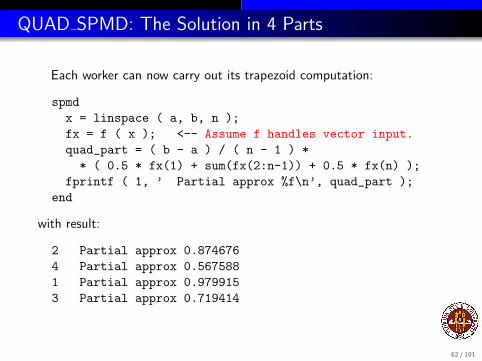
QUAD SPMD: The Solution in 4 Parts
Each worker can now carry out its trapezoid computation:
spmdx = linspace ( a, b, n );fx = f ( x ); <-- Assume f handles vector input.quad_part = ( b - a ) / ( n - 1 ) ** ( 0.5 * fx(1) + sum(fx(2:n-1)) + 0.5 * fx(n) );
fprintf ( 1, ’ Partial approx %f\n’, quad_part );end
with result:
2 Partial approx 0.8746764 Partial approx 0.5675881 Partial approx 0.9799153 Partial approx 0.719414
62 / 101
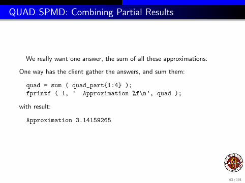
QUAD SPMD: Combining Partial Results
We really want one answer, the sum of all these approximations.
One way has the client gather the answers, and sum them:
quad = sum ( quad_part{1:4} );fprintf ( 1, ’ Approximation %f\n’, quad );
with result:
Approximation 3.14159265
63 / 101
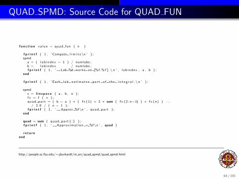
QUAD SPMD: Source Code for QUAD FUN
f u n c t i o n v a l u e = quad fun ( n )
f p r i n t f ( 1 , ’ Compute l i m i t s\n ’ ) ;spmd
a = ( l a b i n d e x − 1 ) / numlabs ;b = l a b i n d e x / numlabs ;f p r i n t f ( 1 , ’ Lab %d works on [%f ,% f ] .\ n ’ , l a b i nd e x , a , b ) ;
end
f p r i n t f ( 1 , ’ Each l a b e s t ima t e s pa r t o f the i n t e g r a l .\n ’ ) ;
spmdx = l i n s p a c e ( a , b , n ) ;f x = f ( x ) ;quad pa r t = ( b − a ) ∗ ( f x (1 ) + 2 ∗ sum ( f x ( 2 : n−1) ) + f x ( n ) ) . . .
/ 2 . 0 / ( n − 1 ) ;f p r i n t f ( 1 , ’ Approx %f\n ’ , quad pa r t ) ;
end
quad = sum ( quad pa r t{:} ) ;f p r i n t f ( 1 , ’ Approx imat ion = %f\n ’ , quad )
r e t u r nend
http://people.sc.fsu.edu/∼jburkardt/m src/quad spmd/quad spmd.html
64 / 101

MATLAB Parallel Computing
Introduction
QUAD Example (PARFOR)
MD Example
PRIME Example
ODE Example
SPMD: Single Program, Multiple Data
QUAD Example (SPMD)
DISTANCE Example
CONTRAST Example
CONTRAST2: Messages
Conclusion
65 / 101
DISTANCE: A Classic Problem
Anyone doing highway traveling is familiar with the difficulty ofdetermining the shortest route between points A and B. From a map, it’seasy to see the distance between neighboring cities, but often the bestroute takes a lot of searching.
A graph is the abstract version of a network of cities. Some cities areconnected, and we know the length of the roads between them. Thecities are often called nodes or vertices and the roads are links or edges.Whereas cities are described by maps, we will describe our abstractgraphs using a one-hop distance matrix, which is simply the length of thedirect road between two cities, if it exists.
66 / 101

DISTANCE: An Intercity Map
Here is an example map with the intercity highway distances:
67 / 101

DISTANCE: An Intercity One-Hop Distance Matrix
Supposing we live in city A, our question is, “What is the shortestpossible distance from A to each city on the map?”
Instead of a map, we use a “one-hop distance” matrix OHD[I][J]:
A B C D E FA 0 40 15 ∞ ∞ ∞B 40 0 20 10 25 6C 15 20 0 100 ∞ ∞D ∞ 10 100 0 ∞ ∞E ∞ 25 ∞ ∞ 0 8F ∞ 6 ∞ ∞ 8 0
where ∞ means there’s no direct route between the two cities.
68 / 101

DISTANCE: The Shortest Distance
The map makes it clear that it’s possible to reach every city from city A;we just have to take trips that are longer than “one hop”. In fact, in thiscrazy world, it might also be possible to reach a city faster by taking twohops rather than the direct route. (Look at how to get from city A tocity B, for instance!)
We want to use the information in the map or the matrix to come upwith a distance vector, that is, a record of the shortest possible distancefrom city A to all other cities.
A method for doing this is known as Dijkstra’s algorithm.
69 / 101
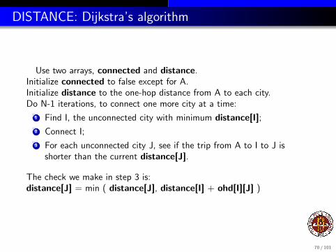
DISTANCE: Dijkstra’s algorithm
Use two arrays, connected and distance.Initialize connected to false except for A.Initialize distance to the one-hop distance from A to each city.Do N-1 iterations, to connect one more city at a time:
1 Find I, the unconnected city with minimum distance[I];
2 Connect I;
3 For each unconnected city J, see if the trip from A to I to J isshorter than the current distance[J].
The check we make in step 3 is:distance[J] = min ( distance[J], distance[I] + ohd[I][J] )
70 / 101

DISTANCE: A Sequential Code
connected(1) = 1;connected(2:n) = 0;
distance(1:n) = ohd(1,1:n);
for step = 2 : n
[ md, mv ] = find_nearest ( n, distance, connected );
connected(mv) = 1;
distance = update_distance ( nv, mv, connected, ...ohd, distance );
end
http://people.sc.fsu.edu/∼jburkardt/m src/dijkstra/dijkstra.html
71 / 101

DISTANCE: Parallelization Concerns
Although the program includes a loop, it is not a parallelizable loop!Each iteration relies on the results of the previous one.
However, let us assume we have a very large number of cities to dealwith. Two operations are expensive and parallelizable:
find nearest searches all nodes for the nearest unconnected one;
update distance checks the distance of each unconnected node tosee if it can be reduced.
These operations can be parallelized by using SPMD statements in whicheach worker carries out the operation for a subset of the nodes. Theclient will need to be careful to properly combine the results from theseoperations!
72 / 101
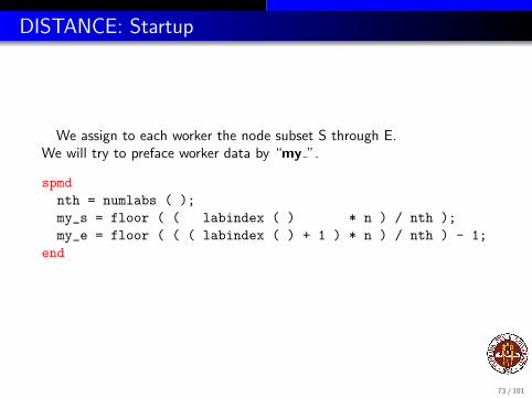
DISTANCE: Startup
We assign to each worker the node subset S through E.We will try to preface worker data by “my ”.
spmdnth = numlabs ( );my_s = floor ( ( labindex ( ) * n ) / nth );my_e = floor ( ( ( labindex ( ) + 1 ) * n ) / nth ) - 1;
end
73 / 101

DISTANCE: FIND NEAREST
Each worker uses find nearest to search its range of cities for thenearest unconnected one.
But now each worker returns an answer. The answer we want is the nodethat corresponds to the smallest distance returned by all the workers, andthat means the client must make this determination.
74 / 101
DISTANCE: FIND NEAREST
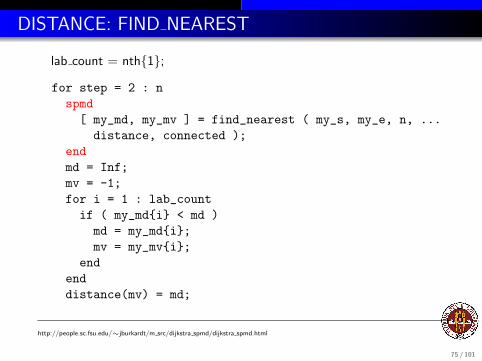
lab count = nth{1};
for step = 2 : nspmd[ my_md, my_mv ] = find_nearest ( my_s, my_e, n, ...distance, connected );
endmd = Inf;mv = -1;for i = 1 : lab_countif ( my_md{i} < md )md = my_md{i};mv = my_mv{i};
endenddistance(mv) = md;
http://people.sc.fsu.edu/∼jburkardt/m src/dijkstra spmd/dijkstra spmd.html
75 / 101

DISTANCE: UPDATE DISTANCE
We have found the nearest unconnected city.
We need to connect it.
Now that we know the minimum distance to this city, we need to checkwhether this decreases our estimated minimum distances to other cities.
76 / 101

DISTANCE: UPDATE DISTANCE
connected(mv) = 1;
spmdmy_distance = update_distance ( my_s, my_e, n, mv, ...connected, ohd, distance );
end
distance = [];for i = 1 : lab_countdistance = [ distance, my_distance{:} ];
end
end
http://people.sc.fsu.edu/∼jburkardt/m src/dijkstra spmd/dijkstra spmd.html
77 / 101
DISTANCE: Comments
This example shows SPMD workers interacting with the client.
It’s easy to divide up the work here. The difficulties come when theworkers return their partial results, and the client must assemble theminto the desired answer.
In one case, the client must find the minimum from a small number ofsuggested values.
In the second, the client must rebuild the distance array from theindividual pieces updated by the workers.
Workers are not allowed to modify client data. This keeps the client datafrom being corrupted, at the cost of requiring the client to manage allsuch changes.
78 / 101
MATLAB Parallel Computing
Introduction
QUAD Example
MD Example
PRIME Example
ODE Example
SPMD: Single Program, Multiple Data
QUAD Example (SPMD)
DISTANCE Example
CONTRAST Example
CONTRAST2: Messages
Conclusion
79 / 101
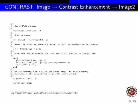
CONTRAST: Image → Contrast Enhancement → Image2
%% Get 4 SPMD worke r s .%
mat labpoo l open l o c a l 4%% Read an image .%
x = imread ( ’ s u r f s u p . t i f ’ ) ;%% Since the image i s b l a c k and white , i t w i l l be d i s t r i b u t e d by columns .%
xd = d i s t r i b u t e d ( x ) ;%% Have each worker enhance the c o n t r a s t i n i t s p o r t i o n o f the p i c t u r e .%
spmdx l = ge tLo c a lPa r t ( xd ) ;x l = n l f i l t e r ( x l , [ 3 , 3 ] , @ad j u s tCon t r a s t ) ;x l = u i n t 8 ( x l ) ;
end%% We are work ing wi th a b l a c k and wh i t e image , so we can s imp l y% conca t ena t e the s ubma t r i c e s to ge t the whole o b j e c t .%
xf spmd = [ x l{:} ] ;
mat l abpoo l c l o s e
http://people.sc.fsu.edu/∼jburkardt/m src/contrast spmd/contrast spmd.html
80 / 101

CONTRAST: Image → Contrast Enhancement → Image2
When a filtering operation is done on the client, we get picture 2. Thesame operation, divided among 4 workers, gives us picture 3. What wentwrong?
81 / 101

CONTRAST: Image → Contrast Enhancement → Image2
Each pixel has had its contrast enhanced. That is, we compute theaverage over a 3x3 neighborhood, and then increase the differencebetween the center pixel and this average. Doing this for each pixelsharpens the contrast.
+-----+-----+-----+| P11 | P12 | P13 |+-----+-----+-----+| P21 | P22 | P23 |+-----+-----+-----+| P31 | P32 | P33 |+-----+-----+-----+
P22 <- C * P22 + ( 1 - C ) * Average
82 / 101
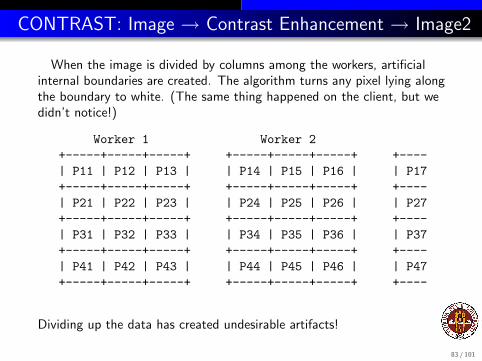
CONTRAST: Image → Contrast Enhancement → Image2
When the image is divided by columns among the workers, artificialinternal boundaries are created. The algorithm turns any pixel lying alongthe boundary to white. (The same thing happened on the client, but wedidn’t notice!)
Worker 1 Worker 2+-----+-----+-----+ +-----+-----+-----+ +----| P11 | P12 | P13 | | P14 | P15 | P16 | | P17+-----+-----+-----+ +-----+-----+-----+ +----| P21 | P22 | P23 | | P24 | P25 | P26 | | P27+-----+-----+-----+ +-----+-----+-----+ +----| P31 | P32 | P33 | | P34 | P35 | P36 | | P37+-----+-----+-----+ +-----+-----+-----+ +----| P41 | P42 | P43 | | P44 | P45 | P46 | | P47+-----+-----+-----+ +-----+-----+-----+ +----
Dividing up the data has created undesirable artifacts!
83 / 101
CONTRAST: Image → Contrast Enhancement → Image2
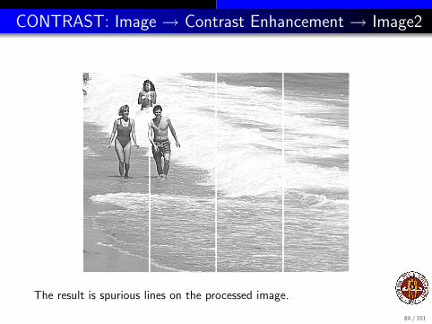
The result is spurious lines on the processed image.
84 / 101

MATLAB Parallel Computing
Introduction
QUAD Example (PARFOR)
MD Example
PRIME Example
ODE Example
SPMD: Single Program, Multiple Data
QUAD Example (SPMD)
DISTANCE Example
CONTRAST Example
CONTRAST2: Messages
Conclusion
85 / 101

CONTRAST2: Workers Need to Communicate
The spurious lines would disappear if each worker could just be allowedto peek at the last column of data from the previous worker, and the firstcolumn of data from the next worker.
Just as in MPI, MATLAB includes commands that allow workers toexchange data.
The command we would like to use is labSendReceive() which controlsthe simultaneous transmission of data from all the workers.
data_received = labSendReceive ( to, from, data_sent );
86 / 101
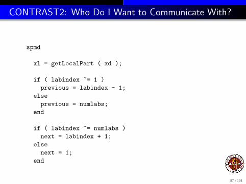
CONTRAST2: Who Do I Want to Communicate With?
spmd
xl = getLocalPart ( xd );
if ( labindex ~= 1 )previous = labindex - 1;
elseprevious = numlabs;
end
if ( labindex ~= numlabs )next = labindex + 1;
elsenext = 1;
end
87 / 101
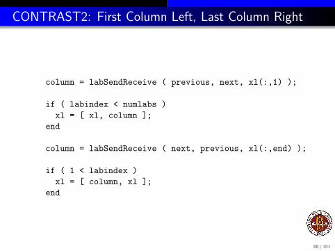
CONTRAST2: First Column Left, Last Column Right
column = labSendReceive ( previous, next, xl(:,1) );
if ( labindex < numlabs )xl = [ xl, column ];
end
column = labSendReceive ( next, previous, xl(:,end) );
if ( 1 < labindex )xl = [ column, xl ];
end
88 / 101

CONTRAST2: Filter, then Discard Extra Columns
xl = nlfilter ( xl, [3,3], @enhance_contrast );
if ( labindex < numlabs )xl = xl(:,1:end-1);
end
if ( 1 < labindex )xl = xl(:,2:end);
end
xl = uint8 ( xl );
end
http://people.sc.fsu.edu/∼jburkardt/m src/contrast2 spmd/contrast2 spmd.html
89 / 101

CONTRAST2: Image → Enhancement → Image2
Four SPMD workers operated on columns of this image.Communication was allowed using labSendReceive.
90 / 101
CONTRAST2: The Heat Equation
Image processing was used to illustrate this example, but consider thatthe contrast enhancement operation updates values by comparing themto their neighbors.
The same operation applies in the heat equation, except that highcontrasts (hot spots) tend to average out (cool off)!
In a simple explicit method for a time dependent 2D heat equation, werepeatedly update each value by combining it with its north, south, eastand west neighbors.
So we could do the same kind of parallel computation, dividing thegeometry into strip, and avoiding artificial boundary effects by havingneighboring SPMD workers exchange “boundary” data.
91 / 101

CONTRAST2: The Heat Equation
The ”east” neighbor lies in the neighboring processor, so its value mustbe received by message in order for the computation to proceed.
92 / 101
CONTRAST2: The Heat Equation
So now it’s time to modify the image processing code to solve the heatequation.
But just for fun, let’s use our black and white image as the initialcondition! Black is cold, white is hot.
In contrast to the contrast example, the heat equation tends to smoothout differences. So let’s watch our happy beach memories fade away ...in parallel ... and with no artificial boundary seams.
93 / 101

CONTRAST2: The Heat Equation, Step 0
94 / 101

CONTRAST2: The Heat Equation, Step 10
95 / 101

CONTRAST2: The Heat Equation, Step 20
96 / 101

CONTRAST2: The Heat Equation, Step 40
97 / 101
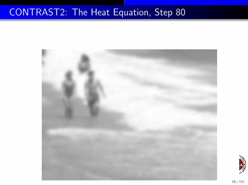
CONTRAST2: The Heat Equation, Step 80
98 / 101

MATLAB Parallel Computing
Introduction
QUAD Example (PARFOR)
MD Example
PRIME Example
ODE Example
SPMD: Single Program, Multiple Data
QUAD Example (SPMD)
DISTANCE Example
CONTRAST Example
CONTRAST2: Messages
Conclusion
99 / 101
Conclusion: A Parallel Version of MATLAB
MATLAB’s Parallel Computing Toolbox allows programmers to takeadvantage of parallel architecture (multiple cores, cluster computers) andparallel programming techniques, to solve big problems efficiently.
MATLAB controls the programming environment; that makes it possibleto send jobs to a remote computer system without the pain of logging in,transferring files, running the program and bringing back the results.MATLAB automates all this for you.
Moreover, when you use the parfor command, MATLAB automaticallydetermines from the form of your loop which variables are to be shared,or private, or are reduction variables; in OpenMP you must recognize anddeclare all these facts yourself.
100 / 101

CONCLUSION: Where is it?
MATLAB Parallel Computing Toolbox User’s Guide 6.0,http://www.mathworks.com/help/pdf doc/distcomp/distcomp.pdf
Gaurav Sharma, Jos Martin,MATLAB: A Language for Parallel Computing,International Journal of Parallel Programming,Volume 37, Number 1, pages 3-36, February 2009.
http://people.sc.fsu.edu/∼jburkardt/presentations/...sem 2012 parfor.pdf (these slides)
http://people.sc.fsu.edu/∼jburkardt/m src/m src.html
quad parformd parforprime parforode sweep parforquad spmddijkstra spmdcontrast spmdcontrast2 spmd
101 / 101