Pareto Monte Carlo Tree Searchfor Multi-Objective Informative Planning

Weizhe Chen, Lantao Liu

Abstract—In many environmental monitoring scenarios, thesampling robot needs to simultaneously explore the environmentand exploit features of interest with limited time. We presentan anytime multi-objective informative planning method calledPareto Monte Carlo tree search which allows the robot tohandle potentially competing objectives such as exploration versusexploitation. The method produces optimized decision solutions forthe robot based on its knowledge (estimation) of the environmentstate, leading to better adaptation to environmental dynamics. Weprovide algorithmic analysis on the critical tree node selection stepand show that the number of times choosing sub-optimal nodesis logarithmically bounded and the search result converges to theoptimal choices at a polynomial rate.

I. INTRODUCTION

There is an increasing need that mobile robots are tasked togather information from our environment. Navigating robots tocollect samples with the largest amount of information is calledinformative planning [4, 21, 25]. The basic idea is to maximizeinformation gain using information-theoretic methods, wherethe information gain (or informativeness) is calculated fromthe estimation uncertainty based on some prediction modelssuch as the set of Gaussian systems. Informative planning ischallenging due to the large and complex searching space. Suchproblems have been shown to be NP-hard [26] or PSPACE-hard [23] depending on the form of objective functions and thecorresponding searching space.

Existing informative planning work is heavily built uponinformation-theoretic framework. The produced solutions tendto guide the robot to explore the uncertain or unknown areas andreduce the estimation uncertainty (e.g., the entropy or mutualinformation based efforts). Aside from the estimation uncer-tainty, there are many other estimation properties that we areinterested in. For example, when monitoring some biologicalactivity in a lake, scientists are interested in areas with highconcentration – known as hotspots – of biological activity [20].Similarly, plume tracking is useful for detection and descriptionof oil spills, thermal vents, and harmful algal blooms [29].In these tasks, the robot needs to explore the environmentto discover hotspots first, and then visit different areas withdiffering effort (frequency) to obtain the most valuable samplesand catch up with the (possibly) spatiotemporal environmentaldynamics.

Since exploration and exploitation cannot be achieved si-multaneously most of the time, different planning objectivesmay lead to distinct motion trajectories. The problem falls

W. Chen and L. Liu are with the School of Informatics, Computing, andEngineering at Indiana University, Bloomington, IN 47408, USA. E-mail:{chenweiz, lantao}@iu.edu.

(a) Bathymetry (b) Example trajectory

Fig. 1. Illustrative multi-objective informative planning trajectory for modelingthe Bathymetry of New Zealand’s Exclusive Economic Zone. The goal is toexplore the environment while visiting areas with high value and variabilitymore frequently. (Source: NIWA)

within the spectrum of multi-objective optimization in whichthe optima are not unique. In fact, continua of optimal solutionsare possible. The goal is to find the Pareto optimal set, or socalled Pareto front. The solutions in the Pareto optimal setcannot be improved for any objective without hurting otherobjectives. A straightforward solution to the multi-objectiveproblem is to convert it into a single-objective problem bylinear scalarization (weighted sum of objectives is one ofthe linear scalarization method). However, linear scalarizationmight be impossible, infeasible, or undesirable for the followingreasons. First of all, objectives might be conflicting. Takingalgal bloom monitoring as an example, high-concentration areasand the areas with high temporal variability (i.e., spreadingdynamics) are both important. We expect the robot to visitthese areas more frequently, but these two types of areas arenot necessarily in the same direction. Furthermore, the weightsamong different objectives are hard to determine in the linearscalarization approaches. Last but not least, linear scalarizationbased approaches fail to discover the solutions in the non-convex regions of the Pareto front.

This paper presents the following contributions:

• Different from existing informative planning approacheswhere information-seeking is the main objective, we pro-pose a new generic planning method that optimizes overmultiple (possibly) competing objectives and constraints.

• We incorporate the Pareto optimization into the MonteCarlo tree search process and further design an anytimeand non-myopic planner for in-situ decision-making.

• We provide in-depth algorithmic analysis which revealsbounding and converging behaviors of the search process.

• We perform thorough simulation evaluations with bothsynthetic and real-world data. Our results show that therobot exhibits desired composite behaviors which are

arX

iv:2

111.

0182

5v1

[cs

.RO

] 2

Nov

202

1

optimized from corresponding hybrid objectives.

II. RELATED WORK

Informative planning maximizes the collected information(informativeness) by exploring (partially) unknown environ-ment during its sampling process [4, 17]. Comparing withthe lawnmower based sweeping style sampling mechanismwhich focuses on spatial resolution, the informative planningmethod tends to achieve the spatial coverage quickly withthe least estimation uncertainty [25]. Due to these reasons,the information planning has been widely used for the spa-tiotemporal environmental monitoring. To explore and learnthe environment model, a commonly-used approach in spatialstatistics is the Gaussian Process Regression [22]. Built on thelearned environmental model, path and motion control can becarried out which is a critical ability for autonomous robotsoperating in unstructured environments [9, 16].

Representative informative planning approaches include, e.g.,algorithms based on a recursive-greedy style [21, 25] where theinformativeness is generalized as submodular function and asequential-allocation mechanism is designed in order to obtainsubsequent waypoints. This recursive-greedy framework hasbeen extended later by incorporating obstacle avoidance anddiminishing returns [4]. In addition, a differential entropy basedframework [17] was proposed where a batch of waypoints canbe obtained through dynamic programming. Recent work alsoreveals that online informative planning is possible [18]. Thesampling data is thinned based on their contributions learnedby a sparse variant of Gaussian Process. There are also methodsoptimizing over complex routing constraints (e.g., see [27, 31]).

Pareto optimization has been used in designing motion plan-ners to optimize over the length of a path and the probabilityof collisions [6]. Recently, a sampling based method has alsobeen proposed to generate Pareto-optimal trajectories for multi-objective motion planning [15]. In addition, multi-robot coor-dination also benefits from multi-objective optimization. Thegoals of different robots are simultaneously optimized [8, 14].To balance the operation cost and the travel discomfort expe-rienced by users, the multi-objective fleet routing algorithmscompute the Pareto-optimal fleet operation plans [5].

Related work also includes the multi-objective reinforce-ment learning [24]. Particularly, the prior work multi-objectiveMonte Carlo tree search (MO-MCTS) is closely relevant toour method [30]. Unfortunately, MO-MCTS is computationallyprohibitive and cannot be used for online planning framework.Vast computational resources are needed in order to maintaina global Pareto optimal set with all the best solutions obtainedso far. In contrast, we develop a framework that maintainsa local approximate Pareto optimal set in each node whichcan be processed in a much faster way. Our approach is alsoflexible and adaptive with regards to capturing environmentalvariabilities of different stages.

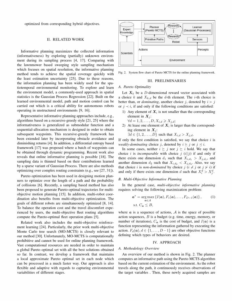
Fig. 2. System flow chart of Pareto MCTS for the online planning framework.

III. PRELIMINARIES

A. Pareto Optimality

Let Xk be a D-dimensional reward vector associated witha choice k and Xk,d be the d-th element. The i-th choice isbetter than, or dominating, another choice j, denoted by i � jor j ≺ i, if and only if the following conditions are satisfied:

1) Any element of Xi is not smaller than the correspondingelement in Xj :∀d = 1, 2, . . . , D,Xi,d > Xj,d;

2) At lease one element of Xi is larger than the correspond-ing element in Xj :∃d ∈ {1, 2, . . . , D} such that Xi,d > Xj,d.

If only the first condition is satisfied, we say that choice i isweakly-dominating choice j, denoted by i � j or j � i.

In some cases, neither i � j nor j � i hold. We say thatchoice i is incomparable with choice j (i||j) if and only ifthere exists one dimension d1 such that Xi,d1 > Xj,d1 , andanother dimension d2 such that Xi,d2

< Xj,d2. Also, we say

that choice i is non-dominated by choice j (i ⊀ j or j � i) ifand only if there exists one dimension d such that Xd

i > Xdj .

B. Multi-Objective Informative Planning

In the general case, multi-objective informative planningrequires solving the following maximization problem:

a∗ = arg maxa∈A

{I(a), F1(a), . . . , FD−1(a)} , (1)

s.t. Ca ≤ B,

where a is a sequence of actions, A is the space of possibleaction sequences, B is a budget (e.g. time, energy, memory, ornumber of iterations), Ca is the cost of budget, and I(a) is afunction representing the information gathered by executing theaction. Fd(a), d ∈ {1, . . . , D−1} are other objective functionsdefining which types of behaviors are desired.

IV. APPROACH

A. Methodology Overview

An overview of our method is shown in Fig. 2. The plannercomputes an informative path using the Pareto MCTS algorithmbased on the current estimation of the environment. As the robottravels along the path, it continuously receives observations ofthe target variables . Then, these newly acquired samples are

Fig. 3. Illustration of main steps of Pareto Monte Carlo tree search (Pareto MCTS).

used to refine its estimation of the environment, which in turninfluences the planning in the next round.

The specific form of rewards depend on the applications.For example, in the informative planning problem, the rewardscan be defined as the reduced amount of estimation entropy,accumulated amount of mutual information, etc. In hotspotexploration and exploitation task, the reward of a given path canbe defined as the sum of rewards of all sampling points alongthe path. Pareto MCTS searches for the optimal actions forcurrent state until a given time budget is exhausted. The inputsof Pareto MCTS are a set of available primitive paths at everypossible state and the robot’s current knowledge (estimation) ofthe world. It is worth noting that, the multi-objective frameworkalso allows us to incorporate prior knowledge, as illustrated onthe left side of Fig. 2.

B. Pareto Monte Carlo Tree Search

The proposed Pareto Monte Carlo tree search (Pareto MCTS)is a planning method for finding Pareto optimal decisions withina given horizon. The tree is built incrementally in order toexpand the most promising subtrees first. This is done by takingadvantage of the information gathered in previous steps. Eachnode in the search tree represents a state of the domain (in ourcontext it is a location to be sampled), and the edges representactions leading to subsequent states.

The framework of Pareto MCTS is outlined in Fig. 3. In eachiteration, it can be broken down into four main steps:

1) Selection: starting at the root node, a child node selec-tion policy (described later on) is applied recursively todescend through the tree until an expandable node withunvisited (unexpanded) children is encountered.

2) Expansion: an action is chosen from the aforementionedexpandable node. A child node is constructed accordingto this action and connected to the expandable node.

3) Simulation: a simulation is run from the new node basedon the predefined default policy. In our case, the defaultpolicy chooses a random action from all available actions.The reward vector of this simulation is then returned.

4) Backpropagation: the obtained reward is backed up orbackpropagated to each visited node in the selection andexpansion steps to update the attributes in those nodes.In our algorithm, each node stores the number of times ithas been visited and the cumulative reward obtained by

simulations starting from this node.These steps are repeated until the maximum number of itera-tions is reached or a given time limit is exceeded.

The most challenging part of designing Pareto MCTS is theselection step. We want to select the most promising nodeto expand first in order to improve the searching efficiency.However, which node is the most promising is unknown so thatthe algorithm needs to estimate it. Therefore, in the selectionstep, one must balance exploitation of the recently discoveredmost promising child node and exploration of alternativeswhich may turn out to be a superior choice at later time.

In the case of scalar reward, the most promising node issimply the one with highest expected reward. However, thereward is herein a vector corresponding to multiple objectives.In the context of multi-objective optimization, the optima areno longer unique. Instead, there is a set of optimal choices,each of which is considered equally best. Below we define thePareto optimal node set. The nodes in the Pareto optimal setare incomparable to each other and will not be dominated byany other nodes.

Definition 1 (Pareto Optimal Node Set). Given a set of nodesV , a subset P∗ ⊂ V is the Pareto optimal node set, in terms ofexpected reward, if and only if{

∀v∗i ∈ P∗ and ∀vj ∈ V, v∗i ⊀ vj ,

∀v∗i , v∗j ∈ P∗, v∗i ||v∗j .

We treat the node selection problem as a multi-objectivemulti-armed bandit problem. As shown in Alg. 1, the ParetoUpper Confidence Bound (Pareto UCB) for each child nodeis first computed according to Eq. (2). Then an approximatePareto optimal set is built using the resulting Pareto UCBvectors (see the green nodes in Fig. 3). Finally, the best childnode is chosen from the Pareto optimal set uniformly at random.Note that the reason for choosing the best child randomlyis that the Pareto optimal solutions are considered equallyoptimal if no preference information is given. However, ifdomain knowledge is available or preference is specified, onecan choose the most preferable child from the Pareto optimalset. For example, in the environmental monitoring task, onemight expect the robot to explore the environment in the earlystage to identify some important areas and spend more effortexploiting these areas in the later stage. In such case, we can

choose the Pareto optimal node with highest information gainin the beginning because the information gain based planningtends to cover the space quickly. Other types of rewards canbe chosen later to concentrate on examining the details locally.

Note that this is different from weighting different objectivesand solve a single-objective problem, because choosing apreferred solution from a given set of optimal solutions is ofteneasier than determining the quantitative relationship amongdifferent objectives. For instance, it is difficult to quantify howmuch the information gain is more important than exploitinghigh-value areas in the hotspot monitoring task. However, givenseveral choices, we may pick the most informative choice inthe very beginning, and another one with highest target valuerelated reward in a later stage.

Algorithm 1: Pareto MCTS

1 Function Search(s0)2 create root node v0 with state s03 while within computational budget do4 vexpandable ← Selection(v0)5 vnew ← Expansion(vexpandable)6 RewardVector← Simulation (vnew.s)7 Backpropagation(vnew,RewardVector)

8 return MostVisitedChild(v0)

9 Function Selection(v)10 while v is fully expanded do11 v ← ParetoBestChild(v)

12 return v

13 Function ParetoBestChild(v)14 compute Pareto UCB for each child k:

U(k) =vk.X

vk.n+

√4 lnn+ lnD

2vk.n(2)

15 build approximate Pareto optimal node set v.Pbased on U(k)

16 choose a child vbest from v.P uniformly at random17 return vbest

18 Note: We use v.attribute to represent a node attribute ofv. In Eq. (2), vk.X is the cumulative reward of thek-th child of node v, vk.n is the number of times thatthe k-th child has been visited, and D is the numberof objectives. Some standard components, such asSimulation, Expansion, and Backpropagation, are notshown due to the lack of space.

C. Algorithm Analysis

As mentioned earlier, the node selection is the most criticalstep and almost determines the performance of the entireframework. Thus, here we spend effort analyzing this stepto better understand its important properties. Although some(potentially) sub-optimal nodes may be selected inevitably, we

show that the number of times choosing a sub-optimal node canbe bounded logarithmically in Pareto MCTS. In addition, wewant to know whether this anytime algorithm will converge tothe optimal solution if enough time is given and whether a goodsolution can be returned if it is stopped midway. To answer thisquestion, we show that the searching result of Pareto MCTSconverges to the Pareto optimal choices at a polynomial rate.

Problem 1 (Node Selection). Consider a node v with K childnodes in a Pareto Monte Carlo search tree. At decision stepn, a D-dimensional random reward Xk,nk will be returnedafter selecting child vk. Successive selections of child vk yieldrewards Xk,1,Xk,2, . . . , which are drawn from an unknowndistribution with unknown expected reward µk. A policy is analgorithm that chooses a child node based on the sequence ofpast selections and obtained rewards. The goal of a policy isto minimize the number of times choosing a sub-optimal node.

In Pareto MCTS, node selection only happens after allchild nodes have been expanded. In other words, there is aninitialization step in which each node has been selected once.For easy reference, we summarize the node selection policybelow.

Policy 1. Given a node selection problem as Problem 1, chooseeach child node once in the first K steps. After that, build anapproximate Pareto optimal node set based on the followingupper confidence bound vector:

U(k) = Xk,nk +

√4 lnn+ lnD

2nk, (3)

where K is the number of child nodes, nk is the number oftimes child k has been selected so far, Xk,nk is the averagereward obtained from child k, D is the number of dimensionsof the reward, and n =

∑Kk=1 nk.

In the following proof, we shall use the concept of mostdominant optimal node originated from the ε-dominance con-cept [12] of multi-objective optimization. Intuitively, the mostdominant optimal node of a given node is the one in the(estimated) Pareto optimal set which is the “farthest away” fromthe given node.

Definition 2 (Most Dominant Optimal Node). Given a nodevk and a node set V such that ∀vk′ ∈ V, vk′ � vk. For allvk′ ∈ V , there exists exactly one minimum positive constantεk′ such that

εk′ = min{ε|∃d ∈ {1, 2, . . . , D} s.t. µ′k,d + ε > µk,d}.

Let the index of the maximum εk′ be k∗,

k∗ = arg maxk′

εk′ ,

then the most dominant optimal node is vk∗ .

Throughout the paper, symbols related to the most dominantoptimal node will be indexed by a star(∗). As in [11], we allowthe expected average rewards to drift as a function of time andour main assumption is that it will converge pointwise. Here weintroduce two assumptions so that the later proof can exploit.

Assumption 1 (Convergence of Expected Average Rewards).The expectations of the average rewards E[Xk,nk ] convergepointwise to the limit µk for all child nodes:

µk = limnk→∞

E[Xk,nk ]. (4)

For a sub-optimal node vk and its most dominant optimalnode vk∗ from P∗, we define ∆k = µ∗ − µk to denote theirdifference.

Assumption 2. Fix 1 ≤ k ≤ K and 1 ≤ d ≤ D. Let {Fk,t,d}tbe a filtration such that {Xk,t,d}t is {Fk,t,d}-adapted andXk,t,d is conditionally independent of Fk,t+1,d,Fk,t+2,d, . . .given Fk,t−1,d.

For the sake of simplifying the notation, we define µk,nk =E[Xk,nk ] and δk,nk = µk,nk −µk as the residual for the drift.Clearly, limnk→∞ δk,nk = 0. By definition, ∀ξ > 0, ∃N0(ξ)such that ∀nk ≥ N0(ξ), ∀d ∈ {1, 2, . . . , D}, |δk,nk,d| ≤ξ∆k,d/2. We present the first theorem below.

Theorem 1. Consider Policy 1 applied to the node selectionProblem 1. Suppose Assumption 1 is satisfied. Let Tk(n) denotethe number of times child node vk has been selected in the firstn steps. If child node vk is a sub-optimal node (i.e. vk 6∈ P∗),then E[Tk(n)] is logarithmically bounded:

E[Tk(n)] ≤ 8 lnn+ 2 lnD

(1− ξ)2(mink,d

∆k,d)2+N0(ξ) + 1 +

π2

3. (5)

Proof: Proof is provided in Appendix A.The following lemma gives a lower bound on the number of

times each child node being selected.

Lemma 1. There exists positive constant ρ such that∀k, n, Tk(n) ≥ dρ log(n)e.

The upcoming lemma states that the average reward willconcentrate around its expectation after enough node selectionsteps.

Lemma 2 (Tail Inequality). Fix arbitrary η > 0 and let σ =

9√

2 ln(2/η)n . There exists N1(η) such that ∀n ≥ N1(η),∀d ∈

{1, . . . , D}, the following bounds hold true:

P(Xn,d ≥ E[Xn,d] + σ) ≤ η, (6)P(Xn,d ≤ E[Xn,d]− σ) ≤ η. (7)

Correctness of Lemma 1 and Lemma 2 is provided in [11].

Theorem 2 (Convergence of Failure Probability). Consider thenode selection policy described in Algorithm 1 applied to theroot node. Let It be the selected child node and P∗ be thePareto optimal node set. Then,

P(It 6∈ P∗) ≤ Ct− ρ2

(mink,d

∆k,d

36

)2

, (8)

with some constant C. In particular, it holds thatlimt→∞ P(It 6∈ P∗) = 0

Proof: Proof is provided in Appendix B.

(a) (b)

Fig. 4. (a) Environment with hotspots used as ground truth. The heat maprepresents level of interest. (b) Primitive paths for a robot.

Theorem 2 shows that, at the root node, the probability ofchoosing a child node (and corresponding action) which is notin the Pareto optimal set converges to zero at a polynomial rateas the number of node selection grows.

V. EXPERIMENTS

To thoroughly evaluate our framework, we have compareddifferent methods in extensive simulations using both syntheticdata and real-world data, where the basic scenario is the hotspotmonitoring task via informative planning for a robot. The idealbehavior for the robot is to first explore the environment todiscover the hotspots and then exploit these important areasto collect more valuable samples. This is a bi-objective taskalthough our algorithm is suitable for multi-objective tasks ingeneral. We choose this scenario for comparison (and illustra-tion) purpose, since one of the comparing methods can onlyhandle bi-objective case. In addition, hotspot monitoring taskcan be easily visualized for interpretation.

We have compared our algorithm with two other baselinemethods. The first method is the Monte Carlo tree search withinformation-theoretic objective, which has been successfullyapplied to planetary exploration mission [1], environment ex-ploration [2, 7], and monitoring spatiotemporal process [19].We called the method information MCTS. The second methodis a upper confidence bound based online planner [28] whichbalances exploration and exploitation in a near-optimal mannerwith appealing no-regret properties. However, when choosingan optimal trajectory, only the primitive paths of current stateare considered in their model. For comparison, we modify andextend this model to MCTS by using the upper confidencebound (see section IV of [28]) as the reward function of MCTS,which is called UCB MCTS.

Rewards: As for the reward function, we choose variancereduction as the information-theoretic objective as in [3, 10].The other reward is devised as adding up the predicted valuesof samples along the path, which encourages the robot to visithigh-value areas more frequently.

Metrics: In the informative planning context, our goal isto minimize the root mean square error (RMSE) between theestimated environmental state (using GP prediction) and theground truth. However, in our hotspot monitoring task, we aremore concerned with the modeling errors in high-value areasthan the entire environment. Therefore, a hotspot RMSE is

(a) (b) (c) (d) (e) (f)

Fig. 5. The arrow represents the robot. (a)(c)(e) The line shows the resulting path of each algorithm with the underlying environment as the background.(b)(d)(f) Robot’s estimation of the target value and collected samples. Red represents high value and blue indicates low value. (a)(b) Information MCTS. (c)(d)UCB MCTS. (e)(f) Pareto MCTS.

(a) (b)

(c) (d)

Fig. 6. The resulting error of the three algorithm in the synthetic problem.(a) Root mean square error. (b) Mean absolute error. (c) Hotspot root meansquare error. (d) Hotspot mean absolute error.

employed for better evaluating the “exploitation” performance.We classify the areas with target values higher than the medianas hotspots and calculate the RMSE within these hotspots.In addition, larger errors in unimportant areas are acceptablein this task and RMSE tends to penalize larger errors in auniform way. Therefore, we also evaluate the methods usingmean absolute error (MAE). Similarly, we introduced hotspotMAE to highlight algorithms’ performance in the importantareas. Last but not least, the percentage of samples in hotspotsmeasures the quality of the collected data. Ideally, the robotshould locate the important areas as soon as possible and gathermore valuable samples in these areas. Also, if there are multiplehotpots, the robot should visit as many hotspots as possibleinstead of getting stuck in one specific area.

A. Synthetic Problems

The robot is tasked to monitor several hotspots in an un-known 10 km × 10 km environment, illustrated in Fig. 4a.

The hotspots to be monitored are specified by three Gaussiansources with random placement and parameters. At each posi-tion, the robot has 15 Dubins paths [13] as its primitive paths.Fig. 4b illustrates an example of available primitive paths.

(a) (b)

Fig. 7. (a) CDOM raw data of Gulf of Mexico. (b) A cropped region nearLouisiana Wetlands.

Fig. 5 shows the the ground truth and prediction with therobot’s path and collected samples. As expected, the informa-tion MCTS tends to cover the whole space and collect thesamples uniformly, because less information will be gainedfrom a point once it has been observed. On the contrary,UCB MCTS spent a small amount of effort exploring theenvironment during the initial phase in order to reduce theuncertainty of the hotspot estimation. After that, it tends togreedily wander around the high-value areas. This phenomenonis consistent with the behavior of the UCB algorithm in themulti-armed bandit problem in which the best machine willbe played much more times than sub-optimal machines. Wenoticed that the bias term in UCB-replanning [28] also increaseswith the mission time, which means that, given enough time,the robot will still try to explore other areas. However, in ourexperiments, the task duration could not be set too long due tothe scalability of the GP. Pareto MCTS simultaneously optimizeall the objectives. As a result, more samples can be found inthe upper hotspot (see Fig. 5f and Fig. 5d).

Fig. 6 presents the global error and hotspot error. The differ-ence between the global error and the hotspot error is negligiblebecause the most important variability is concentrated in thehotspot areas. We notice that, in the first 200 samples, theperformance of Pareto MCTS is inferior to other two methods.In fact, this is because Pareto MCTS has not yet discovered anyparticular hotspot in the initial exploration phase. Once it findsthe a hotspot and starts exploiting that hotspot, the error curve

(a) (b)

(c) (d)

(e) (f)

Fig. 8. The resulting path, collected samples, and prediction of each algorithmin the chromophoric dissolved organic material monitoring problem. Blue andred correspond to low and high value, respectively. The arrow represents therobot and the crosses are the sampled data. (a) Path and the ground truth ofinformation MCTS. (b) Collected samples and the estimated hotspot map frominformation MCTS. (c) Path and the ground truth of UCB MCTS. (d) Collectedsamples and estimation of UCB MCTS. (e) Path and the ground truth of ParetoMCTS. (f) Collected samples and estimation of Pareto MCTS.

drops drastically, surpassing the other two methods at about 300samples. This property is consistent with our motivation. It isalso obvious that our method in general has the steepest errorreduction rate, which is particularly important in monitoringhighly dynamic environment.

B. Chromophoric Dissolved Organic Material Monitoring

We now demonstrate our proposed approach using the chro-mophoric dissolved organic material (CDOM) data at the Gulfof Mexico, provided by National Oceanic and AtmosphericAdministration (NOAA). The concentration of CDOM has asignificant effect on biological activity in aquatic systems. Veryhigh concentrations of CDOM can affect photosynthesis andinhibit the growth of phytoplanktons. Fig. 7a is the raw data

(a) (b)

Fig. 9. The root mean square error and mean absolute error of the threealgorithms in the chromophoric dissolved organic material monitoring problem.(a) Root mean square error. (b) Mean absolute error. The blue line is visuallyoverlapped with the green line. They are separated after zooming in, but thedifference is negligible.

Fig. 10. Percentage of hotspot samples of the three algorithms in thechromophoric dissolved organic material monitoring problem.

of CDOM. We have cropped a smaller region with a highervariability of the target value (Fig. 7b). Due to the scalabilityissue of the GP, the raw data (300×300 grids) is down-sampledto (30× 30).

Fig. 8 reveals similar sample distribution patterns as in thesynthetic data. Specifically, the information MCTS featuresgood spatial coverage. UCB MCTS prefers to stay at thehotspot with highest target value after a rough exploration ofthe environment. Pareto MCTS tends to compromise betweenhotspot searching and hotspot close examination. As a result,it exhibits interesting winding paths in some important areas(see Fig. 8f). This allows the robot to collect more samples inthose areas without losing too much information gain.

In this experiment, we also show how to incorporate priorknowledge in the Pareto MCTS. In robotic environmental mon-itoring, the robot needs to explore the environment extensivelyin the early stage. To this end, we always choose the mostinformative action from the Pareto optimal set at the beginning(first 400 samples), which makes Pareto MCTS degenerateto information MCTS. As shown in Fig. 9, the root meansquare error of information MCTS (blue line) and that of ParetoMCTS (green line) visually overlap. This implies that there isalmost no loss in global modeling error. At the same time, thepercentage of samples collected from hotspots has increased.Fig. 10 shows the percentage of hotspot samples. These resultsvalidate the benefits of multi-objective informative planning andPareto MCTS.

VI. CONCLUSIONThis paper presents a Pareto multi-objective optimization

based informative planning approach. We show that the search-ing result of Pareto MCTS converges to the Pareto optimalactions at a polynomial rate, and the number of times choosinga sub-optimal node in the course of tree search has a logarithmicbound. Our method allows the robot to adapt to the targetenvironment and adjust its concentrations on environmentalexploration versus exploitation based on its knowledge (estima-tion) of the environment. We validate our approach in a hotspotmonitoring task using real-world data and the results reveal thatour algorithm enables the robot to explore the environmentand, at the same time, visit hotspots of high interests morefrequently.

APPENDIXA. Proof to Theorem 1

Let variable It be the index of the selected child node atdecision step t and 1{·} be a Boolean predicate function. Letthe bias term in Eq. (3) be ct,s =

√4 ln t+lnD

2s . Then ∀l >0 and l ∈ Z+, for any sub-optimal node vk, we have the upperbound Tk(n).

Tk(n) =l +

n∑t=K+1

1{It = k}

≤l +

n∑t=K+1

1{It = k, Tk(t− 1) ≥ l}

≤l +

n∑t=K+1

1{X∗Tj(t−1) + ct−1,T∗(t−1)

� Xk,Tk(t−1) + ct−1,Tk(t−1), Tk(t− 1) ≥ l}

≤l +

∞∑t=1

t−1∑s=1

t−1∑sk=l

1{X∗s + ct,s � Xk,sk + ct,sk}

X∗s + ct,s � Xk,sk + ct,sk implies that at least one of thefollowing must hold:

X∗s � µ∗s − ct,s (9)Xk,sk ⊀ µk,sk − ct,s (10)µ∗s � µk,s + 2ct,sk (11)

Otherwise, If Eq. (9), (10) are false, then Eq. (11) is true.We bound the probability of events Eq. (9) (10) using

Chernoff-Hoeffding Bound and Union Bound.

P(X∗s � µ∗s − ct,s)=P((X∗s,1 < µ∗s,1 − ct,s) ∨ · · · ∨ (X∗s,D < µ∗s,D − ct,s)

)≤

D∑d=1

P(X∗s,d < µ∗s,d − ct,s

)(Union Bound)

≤D∑d=1

1

Dt−4 = t−4 (Chernoff-Hoeffding Bound)

Similarly, P(Xi,sk ⊀ µi,sk − ct,s) ≤ t−4Let

l = max

⌈

8 ln t+ 2 lnD

(1− ξ)2 mink,d

∆2k,d

⌉, N0(ξ)

.

Since sk,d ≥ l0, (11) is false.Therefore, plugging the above results into the bound on

Tk(n) and taking expectations of both sides, we get

E[Tk(n)] ≤⌈

8 ln t+ 2 lnD

(1− ξ)2 mink,d

∆2k,d

⌉+N0(ξ) +

∞∑t=1

t−1∑s=1

t−1∑sk=l(

P(X∗s � µ∗s − ct,s) + P(Xk,sk ⊀ µk,sk − ct,s))

≤ 8 ln t+ 2 lnD

(1− ξ)2 mind

∆2k,d

+N0(ξ) + 1 +π2

3,

which concludes the proof.

B. Proof to Theorem 2

Let k be the index of a sub-optimal node. Then P(It 6∈ P∗) ≤∑vk 6∈P∗ P

(Xk,Tk(t) ⊀ X∗T∗(t)

). Note that Xk,Tk(t) ⊀ X∗T∗(t)

implies

Xk,Tk(t) ⊀ µk +∆k

2, (12)

orX∗T∗(t) � µ

∗ +∆k

2. (13)

Otherwise, suppose Eq. (12) and (13) do not hold, we haveXk,Tk(t) ≺ X∗T∗(t) which yields a contradiction. Hence,

P(Xk,Tk(t) ⊀ X

∗T∗(t)

)≤P(Xk,Tk(t) ⊀ µk +

∆k

2)︸ ︷︷ ︸

first term

+P(X∗T∗(t) � µ∗ +

∆k

2)︸ ︷︷ ︸

second term

.

Here we show how to bound the first term:

P(Xk,Tk(t) ⊀ µk +∆k

2)

≤D∑d=1

P(Xk,Tk(t),d > µk,d +∆k,d

2) (Union Bound)

≤D∑d=1

P(Xk,Tk(t),d ≥ µk,Tk(t),d − |δk,Tk(t),d|︸ ︷︷ ︸converges to 0

+∆k,d

2)

≤D∑d=1

P(Xk,Tk(t),d ≥ µk,Tk(t),d +∆k,d

4)

≤D∑d=1

constant(1

t)

ρ2

(mink,d

∆k,d

36

)2

(Lemma 2)

The last step makes use of Lemma 1 and Lemma 2.The second term can be bounded in a similar way. Finally,

an integration of the bounds shows that the failure probabilityconverges to 0 at a polynomial rate as the number of selectiongoes to infinity.

REFERENCES

[1] Akash Arora, Robert Fitch, and Salah Sukkarieh. Anapproach to autonomous science by modeling geologicalknowledge in a bayesian framework. In IEEE/RSJ In-ternational Conference on Intelligent Robots and Systems(IROS), pages 3803–3810. IEEE, 2017.

[2] Graeme Best, Oliver M Cliff, Timothy Patten, Ram-gopal R Mettu, and Robert Fitch. Dec-mcts: Decentralizedplanning for multi-robot active perception. The Inter-national Journal of Robotics Research, 38(2-3):316–337,2019.

[3] Jonathan Binney and Gaurav S Sukhatme. Branch andbound for informative path planning. In IEEE Inter-national Conference on Robotics and Automation, pages2147–2154. IEEE, 2012.

[4] Jonathan Binney, Andreas Krause, and Gaurav S.Sukhatme. Optimizing waypoints for monitoring spa-tiotemporal phenomena. International Journal onRobotics Research (IJRR), 32(8):873–888, 2013.

[5] Michal Cap and Javier Alonso-Mora. Multi-objectiveanalysis of ridesharing in automated mobility-on-demand.In Robotics: Science and Systems, 2018.

[6] Shushman Choudhury, Christopher M Dellin, and Sid-dhartha S Srinivasa. Pareto-optimal search over config-uration space beliefs for anytime motion planning. InIEEE/RSJ International Conference on Intelligent Robotsand Systems (IROS), pages 3742–3749. IEEE, 2016.

[7] Micah Corah and Nathan Michael. Efficient online multi-robot exploration via distributed sequential greedy assign-ment. In Proceedings of robotics: science and systems,2017.

[8] Robert Ghrist, Jason M O’Kane, and Steven M LaValle.Pareto optimal coordination on roadmaps. In Algorithmicfoundations of robotics VI, pages 171–186. Springer,2004.

[9] Carlos Ernesto Guestrin. Planning Under Uncertainty inComplex Structured Environments. PhD thesis, Stanford,CA, USA, 2003. AAI3104233.

[10] Geoffrey A Hollinger and Gaurav S Sukhatme. Sampling-based robotic information gathering algorithms. TheInternational Journal of Robotics Research, 33(9):1271–1287, 2014.

[11] Levente Kocsis and Csaba Szepesvari. Bandit basedmonte-carlo planning. In European conference on ma-chine learning, pages 282–293. Springer, 2006.

[12] Joshua B Kollat, Patrick M Reed, and Joseph R Kasprzyk.A new epsilon-dominance hierarchical bayesian optimiza-tion algorithm for large multiobjective monitoring networkdesign problems. Advances in Water Resources, 31(5):828–845, 2008.

[13] Steven M LaValle. Planning algorithms. Cambridgeuniversity press, 2006.

[14] Steven M LaValle and Seth A Hutchinson. Optimalmotion planning for multiple robots having independentgoals. IEEE Transactions on Robotics and Automation,

14(6):912–925, 1998.[15] Jeongseok Lee, Daqing Yi, and Siddhartha S Srinivasa.

Sampling of pareto-optimal trajectories using progressiveobjective evaluation in multi-objective motion planning. InIEEE/RSJ International Conference on Intelligent Robotsand Systems (IROS), pages 1–9. IEEE, 2018.

[16] Naomi E Leonard, Derek A Paley, Russ E Davis, David MFratantoni, Francois Lekien, and Fumin Zhang. Coordi-nated control of an underwater glider fleet in an adaptiveocean sampling field experiment in monterey bay. Journalof Field Robotics, 27(6):718–740, 2010.

[17] Kian Hsiang Low. Multi-robot Adaptive Exploration andMapping for Environmental Sensing Applications. PhDthesis, Carnegie Mellon University, Pittsburgh, PA, USA,2009.

[18] Kai-Chieh Ma, Lantao Liu, Hordur K Heidarsson, andGaurav S Sukhatme. Data-driven learning and planningfor environmental sampling. Journal of Field Robotics,35(5):643–661, 2018.

[19] Roman Marchant, Fabio Ramos, Scott Sanner, et al. Se-quential bayesian optimisation for spatial-temporal moni-toring. In UAI, pages 553–562, 2014.

[20] Seth McCammon and Geoffrey A Hollinger. Topologicalhotspot identification for informative path planning witha marine robot. In IEEE International Conference onRobotics and Automation (ICRA), pages 1–9. IEEE, 2018.

[21] Alexandra Meliou, Andreas Krause, Carlos Guestrin, andJoseph M. Hellerstein. Nonmyopic informative pathplanning in spatio-temporal models. In Proceedings ofNational Conference on Artificial Intelligence (AAAI),pages 602–607, 2007.

[22] Carl Edward Rasmussen and Christopher K. I. Williams.Gaussian Processes for Machine Learning. The MITPress, 2005.

[23] John H Reif. Complexity of the mover’s problem and gen-eralizations. In 20th Annual Symposium on Foundationsof Computer Science, pages 421–427, 1979.

[24] Diederik M Roijers, Peter Vamplew, Shimon Whiteson,and Richard Dazeley. A survey of multi-objective sequen-tial decision-making. Journal of Artificial IntelligenceResearch, 48:67–113, 2013.

[25] Amarjeet Singh, Andreas Krause, Carlos Guestrin,William Kaiser, and Maxim Batalin. Efficient planningof informative paths for multiple robots. In Proceedingsof the 20th International Joint Conference on ArtificalIntelligence, pages 2204–2211, 2007.

[26] Amarjeet Singh, Andreas Krause, Carlos Guestrin, andWilliam J Kaiser. Efficient informative sensing using mul-tiple robots. Journal of Artificial Intelligence Research,34:707–755, 2009.

[27] Daniel E Soltero, Mac Schwager, and Daniela Rus. Gener-ating informative paths for persistent sensing in unknownenvironments. In 2012 IEEE/RSJ International Confer-ence on Intelligent Robots and Systems, pages 2172–2179.IEEE, 2012.

[28] Wen Sun, Niteesh Sood, Debadeepta Dey, Gireeja Ranade,Siddharth Prakash, and Ashish Kapoor. No-regret replan-ning under uncertainty. In IEEE International Conferenceon Robotics and Automation (ICRA), pages 6420–6427.IEEE, 2017.

[29] Sara Susca, Francesco Bullo, and Sonia Martinez. Moni-toring environmental boundaries with a robotic sensor net-work. IEEE Transactions on Control Systems Technology,16(2):288–296, 2008.

[30] Weijia Wang and Michele Sebag. Multi-objective monte-carlo tree search. In Asian conference on machine learn-ing, volume 25, pages 507–522, 2012.

[31] Jingjin Yu, Mac Schwager, and Daniela Rus. Correlatedorienteering problem and its application to informativepath planning for persistent monitoring tasks. In IEEE/RSJInternational Conference on Intelligent Robots and Sys-tems, pages 342–349. IEEE, 2014.