ParCrunchFlow: an efficient, parallel reactive transport...

AUTHOR'S PROOF JrnlID 10596 ArtID 9475 Proof#1 - 20/03/2015

UNCORRECTEDPROOF

Comput GeosciDOI 10.1007/s10596-015-9475-x

ORIGINAL PAPER1

ParCrunchFlow: an efficient, parallel reactive transportsimulation tool for physically and chemically heterogeneoussaturated subsurface environments

2

3

4

James J. Beisman1 · Reed M. Maxwell1 · Alexis K. Navarre-Sitchler1 ·Carl I. Steefel2 · Sergi Molins2

5

6

Received: 27 May 2014 / Accepted: 27 February 20157© Springer International Publishing Switzerland 20158

Abstract Understanding the interactions between physical,9

geochemical, and biological processes in the shallow sub-10

surface is integral to the development of effective contam-11

ination remediation techniques, or the accurate quantifica-12

tion of nutrient fluxes and biogeochemical cycling. Hydrol-13

ogy has a primary control on the behavior of shallow subsur-14

face environments and must be realistically represented if15

we hope to accurately model these systems. ParCrunchFlow16

is a new parallel reactive transport model that was created17

by coupling a multicomponent geochemical code (Crunch-18

Flow) with a parallel hydrologic model (ParFlow). These19

models are coupled in an explicit operator-splitting manner.20

ParCrunchFlow can simulate three-dimensional multicom-21

ponent reactive transport in highly resolved, field-scale sys-22

tems by taking advantage of ParFlow’s efficient parallelism23

and robust hydrologic abilities, and CrunchFlow’s extensive24

geochemical abilities. Here, the development of ParCrunch-25

Flow is described and two simple verification simulations26

are presented. The parallel performance is evaluated and27

shows that ParCrunchFlow has the ability to simulate very28

large problems. A series of simulations involving the biolog-29

ically mediated reduction of nitrate in a floodplain aquifer30

were conducted. These floodplain simulations show that this31

code enables us to represent more realistically the variabil-32

ity in chemical concentrations observed in many field-scale

Q1

33

! James J. [email protected]

1 Colorado School of Mines,Golden, CO 80401 USA

2 Lawrence Berkeley National Laboratory,Berkeley, CA 94720 USA

systems. The numerical formulation implemented in Par- 34

CrunchFlow minimizes numerical dispersion and allows the 35

use of higher-order explicit advection schemes. The effects 36

that numerical dispersion can have on finely resolved, field- 37

scale reactive transport simulations have been evaluated. 38

The smooth gradients produced by the first-order scheme 39

create an artificial mixing effect, which decreases the spatial 40

variance in solute concentrations and leads to an increase 41

in overall reaction rates. The work presented here is the 42

first step in a larger effort to couple these models in a 43

transient, variably saturated surface-subsurface framework, 44

with additional geochemical abilities. 45

Keywords Parallel reactive transport · Subsurface nutrient 46

cycling · Biogeochemical reactions 47

1 Introduction 48

Subsurface hydrogeochemical systems are an extremely 49

complex component of the terrestrial environment and 50

play host to a multitude of interacting processes. Dynamic 51

coupled relationships between physical, geochemical, and 52

microbial processes dictate the behavior of these systems. 53

Parameterizations of these processes exhibit strong scale 54

dependence, limiting our ability to extrapolate laboratory 55

results to field scales or other conditions [1–4]. Addition- 56

ally, high levels of spatial variability are often observed 57

in the physical and biogeochemical properties of natural 58

subsurface environments, limiting the ability of analytical 59

solutions or simple models to adequately describe these 60

systems. Developing a thorough understanding of how 61

these coupled physical, chemical, and microbiological pro- 62

cesses interact at field scales is integral to the development 63

of effective contamination remediation techniques, or the 64

mailto:[email protected]


UNCORRECTEDPROOF

Comput Geosci

accurate quantification of nutrient fluxes and biogeochemi-65

cal cycling. Reactive transport modeling has been presented66

as a research approach that can help to integrate and eval-67

uate the effects of these coupled processes in subsurface68

environments [5–7].69

Natural variability in subsurface porous materials leads70

to spatial and temporal heterogeneities in both the physi-71

cal properties [8–10] and the biogeochemical properties [11,72

12] of an aquifer. These heterogeneities heavily influence73

important subsurface reactions [13]. Chemical transport in74

natural systems does not behave according to the trans-75

port laws established for homogeneous systems [7, 14–16].76

In the non-uniform flow fields of natural systems, flow77

tends to preferentially move through continuous pathways78

of higher-permeability material, effectively isolating low-79

permeability portions of the subsurface from the bulk of the80

solute flux [17]. In addition to the complexities involved81

in representing hydrogeochemical systems due to hetero-82

geneities, a mixture of equilibrium and kinetic pathways is83

often required to adequately describe natural systems [18].84

In these systems, multiple reaction pathways to the same85

endpoint commonly exist, and the rate laws and thermo-86

dynamic relationships that describe these pathways involve87

multiple chemical species and are often nonlinear [17].88

The complex nature of these systems necessitates a mod-89

eling approach that can represent heterogeneities in both90

the physical and biogeochemical properties of the subsur-91

face at a fine scale, while incorporating multiple kinetic92

and equilibrium reaction paths. To further our understand-93

ing of the interacting and competing processes involved94

in field-scale reactive transport, we have developed the95

parallel reactive transport code ParCrunchFlow. This code96

is a coupling of the parallel groundwater code ParFlow97

and the multicomponent geochemical code CrunchFlow.98

Hydrologic conditions are thought to have a primary con-99

trol on effective reaction rates in field systems [19–22].100

By taking advantage of ParFlow’s robust ability to rep-101

resent domain heterogeneities and complex flow [23–25],102

ParCrunchFlow is better able to represent the interactions103

that occur between realistic, non-uniform flow fields and104

biogeochemical processes. Field-scale reactive transport105

simulations are inherently computationally expensive, as106

domain resolutions must be fine enough to capture small-107

scale heterogeneities and processes such as fingering, and108

the number of chemical components can be quite large.109

ParCrunchFlow can simulate these extremely large prob-110

lems by taking advantage of the efficient parallelism built111

into ParFlow. This is the first step of a larger project to112

create a code tailored for field-scale, high-resolution, sur-113

face to shallow subsurface reactive transport simulations.114

ParCrunchFlow can currently represent reactive transport115

in isothermal, fully saturated, steady-state systems and can116

incorporate many simultaneous reaction pathways. In the117

following sections, we present the details of this coupling, 118

verify the code, and evaluate ParCrunchFlow’s parallel per- 119

formance. A series of simulations involving interactions 120

between solid-phase organic carbon, aqueous oxygen, and 121

nitrogen in a floodplain aquifer are then presented. Finally, 122

we examine the influence that the accuracy of the advec- 123

tion scheme can have in highly resolved systems with a high 124

degree of heterogeneity. 125

2 Model description, governing equations, 126

numerical formulation, and model structure 127

2.1 Model description 128

The following section describes the components of the cou- 129

pled model ParCrunchFlow, the mathematical basis of the 130

model, and the coupling details and program structure. 131

2.1.1 ParFlow 132

ParFlow is a parallel three-dimensional integrated hydro- 133

logic model [26–28]. While ParFlow solves the subsurface 134

flow equations for either transient, variably saturated con- 135

ditions or steady-state, saturated flow conditions, here, the 136

steady-state, saturated version of ParFlow is used, and fur- 137

ther discussion is limited to the processes represented by 138

this version of the model. ParFlow uses a parallel multigrid- 139

preconditioned conjugate gradient method to solve isother- 140

mal, single-phase, steady-state, saturated flow fields [26]. 141

This method provides a computationally accurate and effi- 142

cient solution of hydraulic head in the subsurface. ParFlow 143

employs a domain decomposition method to allow paral- 144

lel computation and has excellent parallel scalability. The 145

ability to take advantage of many processors allows the 146

representation of large domains with finely resolved hetero- 147

geneities. Several geostatistical tools are built into ParFlow, 148

providing a convenient means of stochastic simulation. Two 149

explicit schemes are available to represent solute advection; 150

a first-order accurate upwind scheme and a second-order 151

accurate Godunov scheme. The second-order scheme is an 152

upwind biased, three-dimensional extension of the unsplit 153

Godunov scheme presented in [29]. To control spurious 154

oscillations near concentration fronts, a bilinear slope lim- 155

iter is employed in the x-y plane and a one-dimensional 156

limiter is used in the z dimension. 157

2.1.2 CrunchFlow 158

CrunchFlow is a multicomponent reactive flow and trans- 159

port code [6, 30, 31]. CrunchFlow operates on the con- 160

tinuum assumption and can simulate geochemical pro- 161

cesses from the Darcy scale to field scales. This code 162


UNCORRECTEDPROOF

Comput Geosci

solves systems of chemical reactions with mixed kinetic-163

equilibrium control. The reactions that can be repre-164

sented include kinetically controlled heterogeneous mineral165

dissolution/precipitation reactions, kinetically controlled166

homogenous reactions, and equilibrium-controlled homo-167

geneous reactions. Biologically mediated reactions can be168

represented with rate laws based on Monod-type formula-169

tions, where the rate of reaction is dependent on the presence170

of electron donors and/or acceptors. Two sets of solvers171

are incorporated into CrunchFlow, a global implicit method172

that solves the transport and reaction terms simultaneously173

and an operator-splitting method that solves the transport174

and reaction terms separately. Here, the operator-splitting175

method is used, and further discussion will be limited176

to the processes represented with this solver. CrunchFlow177

can simulate a wide range of important geochemical pro-178

cesses, including but not limited to reactive contaminant179

transport, chemical weathering, carbon sequestration, and180

biogeochemical cycling [22, 32–35].181

2.1.3 The coupled model ParCrunchFlow182

The coupled model ParCrunchFlow was created by com-183

bining the ParFlow steady-state saturated groundwater flow184

and transport solver with the reaction solver from Crunch-185

Flow’s operator-splitting subroutine. This coupling was186

accomplished via the sequential non-iterative approach187

(SNIA) [36–39], whereby the reaction terms in Crunch-188

Flow’s operator-splitting solver were linked to ParFlow’s189

advection formulation. This code can simulate isothermal,190

single-phase reactive solute transport under steady-state191

saturated conditions in complex domains. The current reac-192

tion capabilities of this code include kinetically controlled193

solid-aqueous reactions, kinetically controlled aqueous-194

aqueous reactions, and equilibrium-controlled aqueous-195

aqueous reactions. Equilibrium-controlled solid-aqueous196

reactions may also be simulated by using a fast kinetic197

rate constant. ParCrunchFlow allows a parallel imple-198

mentation of CrunchFlow’s robust geochemical abilities199

coupled with ParFlow’s flow and domain representation200

abilities.201

2.2 Governing equations202

Steady-state, fully saturated groundwater flow is described203

by204

∇ · (K∇h) − q = 0 (1)

where Kis the saturated hydraulic conductivity tensor205

(m s−1), h represents the hydraulic gradient (−), and q is206

a general source/sink term (m s−1). The saturated hydraulic207

conductivity tensor is diagonal and anisotropic K can be208

represented. The velocity of water moving through a flow 209

field described by Eq. 1 is shown here. 210

V = ∇ · (K∇h)

φ(2)

where V is the velocity vector (m s−1) and φ is the porosity 211

of the medium (−). The governing differential equation for 212

advection and reaction in a single-phase system is 213

∂Ci

∂t+ ∇ · (V Ci) − Ri = 0 (i = 1, n) (3)

where Ci is the concentration of species i in solution 214

(mol kgw−1), V is flow velocity, Ri is the total reaction rate 215

of species i in solution (mol kgw−1 s−1), and n is the total 216

number of aqueous species. Note that dispersion and dif- 217

fusion are not represented. This equation is a statement of 218

mass conservation in an advective flow (no diffusion) and 219

incorporates reaction terms. 220

The general formulation for conservation of solute mass 221

given by Eq. 3 makes no assumptions of equilibrium 222

between chemical species. However, if we model a sys- 223

tem where various chemical species are assumed to be in 224

equilibrium with each other, we may reduce the number 225

of independent concentrations in the system and therefore 226

reduce the number of species that must be solved for. This 227

leads to a partitioning of the system into Nc primary and 228

Nx secondary chemical species. The assumption of chemi- 229

cal equilibrium between the primary and secondary species 230

allows us to utilize mass action laws to describe the con- 231

centrations of the secondary species, Xj (mol kgw−1),

Q2

232

233

Xj = K−1j γ −1

j

Nc!

i=1

(γiCi)vij (j = 1, Nx) (4)

where Kj is the thermodynamic equilibrium constant for 234

secondary species j , and γi and γj are the activity coeffi- 235

cients for primary species i and secondary species j . The 236

concentrations of the primary species can then be repre- 237

sented as the free concentration plus the concentration of 238

any associated secondary species [5, 36, 40, 41] 239

Ui = Ci +Nx"

j=1

vijXj (i = 1, Nc) (5)

where Ui is the total concentration of primary species i, 240

Ci is the free concentration of primary species i, Xj are 241

the concentrations of the secondary species that contribute, 242

via equilibrium reactions, to primary species i, and vij are 243

the stoichiometric coefficients of the equilibrium reactions. 244

The governing differential equation can then be expressed 245

in terms of the total concentrations of the primary species 246

∂Ui

∂t+ ∇ · (V Ui) − Ri = 0 (i = 1, Nc) (6)


UNCORRECTEDPROOF

Comput Geosci

This technique offers increased computational efficiency for247

systems with large numbers of reactions that are assumed248

to be at equilibrium by reducing the number of species that249

must be solved for. The reaction term Ri is comprised of250

heterogeneous mineral dissolution/precipitation reactions,251

Rmini , and homogeneous aqueous reactions, R

aqi252

Ri = Rmini + R

aqi (7)

The solid-phase reaction term Rmini can be defined as253

the sum of all the mineral reactions that involve primary254

species i255

Rmini = −

Nm"

m=1

vmrm (8)

where Nm is the number of mineral reactions that affect pri-256

mary species i, rm is the rate of dissolution or precipitation257

of mineral m, and vm is the stoichiometric coefficient of258

the dissolution reaction for 1 mol of mineral m. The aque-259

ous reaction term, Raqi , takes a form similar to the mineral260

reaction term261

Raqi = −

Nk"

k=1

vkrk (9)

where Nk is the number of kinetic aqueous reactions that262

affect primary species i, rk is the rate of reaction k, and vk263

is the stoichiometric coefficient of reaction k.264

2.3 Kinetic rate laws265

Two types of kinetic rate laws are defined for both mineral266

and aqueous reactions. The first is based on transition state267

theory [42–44]. In the formulation employed here, the rate268

of a given reaction is a function of the ion activity product,269

Q =Ns!

i=1

γ s (10)

where Ns is the number of species involved in the reaction270

and γ s are the activities of the species raised to their sto-271

ichiometric coefficients. For heterogeneous reactions, this272

form of transition state theory takes the form273

R = AmKme

#−EarT

$ !ani

%1 − Qm

Keq

&(11)

where Am is the surface area of mineral m (m2), Km is the274

intrinsic rate constant (mol m−2 s−1), Ea is the activation275

energy, r is the gas constant, T is the temperature in degrees276

kelvin, Qm is the ion activity product of the mineral reac-277

tion, Keq is the thermodynamic equilibrium constant, and278

the product'

ani represents the inhibition or catalysis of279

the reaction by species in solution raised to the power of n.280

For homogeneous aqueous reactions, this rate law takes the 281

form 282

R = ks

!ani

%1 − Qs

Keq

&(12)

where ks is the intrinsic rate constant (mol kgw−1 s−1), and 283

Qs is the ion activity product for the homogeneous reaction. 284

Note that this form does not currently include a temperature 285

dependence. The second type of rate law used here is Monod 286

kinetic theory, which takes the same form for homogenous 287

and heterogeneous reactions. The Monod formulation cal- 288

culates reaction rates based on the concentrations of electron 289

donors and/or acceptors 290

R = kmax

(Ci

Ci + Khalf

)(13)

where Kmax is the maximum reaction rate (mol kgw−1 s−1), 291

Ci is the concentration of the electron donor or accep- 292

tor (mol kgw−1), and Khalf is the half-saturation constant 293

(mol kgw−1). The Monod formulation employed here also 294

accounts for the inhibition of the reaction in the presence of 295

certain species 296

R = kmax

(Ci

Ci + Khalf

)(Kin

Cin + Kin

)(14)

where Kin is the inhibition constant (mol kgw−1), and Cin 297

is the concentration of the inhibiting species (mol kgw−1). 298

The Monod laws presented here assume that biomass con- 299

centrations are constant. Note that all of the rate laws 300

presented here are written in terms of free species con- 301

centrations, Ci , while the transport equation is written in 302

terms of primary species concentrations, Ui . Therefore, a 303

speciation calculation is required to compute the rates. 304

2.4 Numerical formulation 305

Equations 4 and 5 allow the governing equation for advec- 306

tive reactive transport (3) to be solved in terms of the 307

total concentrations of the primary species (6). We employ 308

an operator-splitting method to approximate (6), where 309

the advection terms and reaction terms are decoupled and 310

solved for separately. Within each timestep, the advection 311

calculations are carried out first, followed by the reac- 312

tion calculations. We use ParFlow to calculate the advec- 313

tion terms via a first-order explicit upwind scheme or a 314

second-order explicit Godunov scheme. After the transport 315

calculations are complete, we use CrunchFlow to calcu- 316

late the reaction terms. For a system with Nc primary 317

species, the reaction terms are represented by Nc ordinary 318

differential equations. Within each individual grid cell, this 319

system of equations is solved numerically with the Newton- 320

Raphson iterative method. When solving the reaction sys- 321

tem, CrunchFlow first calculates the secondary species and 322


UNCORRECTEDPROOF

Comput Geosci

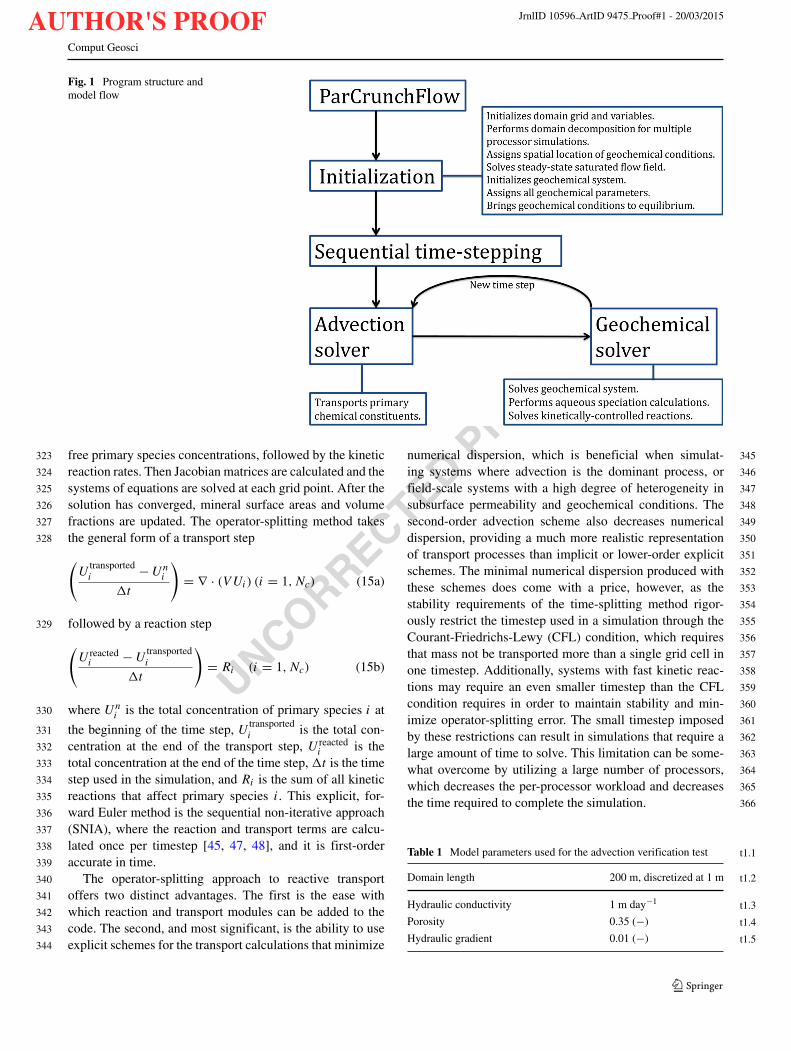
Fig. 1 Program structure andmodel flow

free primary species concentrations, followed by the kinetic323

reaction rates. Then Jacobian matrices are calculated and the324

systems of equations are solved at each grid point. After the325

solution has converged, mineral surface areas and volume326

fractions are updated. The operator-splitting method takes327

the general form of a transport step328

*U

transportedi − Un

i

$t

+

= ∇ · (V Ui) (i = 1, Nc) (15a)

followed by a reaction step329

*U reacted

i − Utransportedi

$t

+

= Ri (i = 1, Nc) (15b)

where Uni is the total concentration of primary species i at330

the beginning of the time step, Utransportedi is the total con-331

centration at the end of the transport step, U reactedi is the332

total concentration at the end of the time step, $t is the time333

step used in the simulation, and Ri is the sum of all kinetic334

reactions that affect primary species i. This explicit, for-335

ward Euler method is the sequential non-iterative approach336

(SNIA), where the reaction and transport terms are calcu-337

lated once per timestep [45, 47, 48], and it is first-order338

accurate in time.339

The operator-splitting approach to reactive transport340

offers two distinct advantages. The first is the ease with341

which reaction and transport modules can be added to the342

code. The second, and most significant, is the ability to use343

explicit schemes for the transport calculations that minimize344

numerical dispersion, which is beneficial when simulat- 345

ing systems where advection is the dominant process, or 346

field-scale systems with a high degree of heterogeneity in 347

subsurface permeability and geochemical conditions. The 348

second-order advection scheme also decreases numerical 349

dispersion, providing a much more realistic representation 350

of transport processes than implicit or lower-order explicit 351

schemes. The minimal numerical dispersion produced with 352

these schemes does come with a price, however, as the 353

stability requirements of the time-splitting method rigor- 354

ously restrict the timestep used in a simulation through the 355

Courant-Friedrichs-Lewy (CFL) condition, which requires 356

that mass not be transported more than a single grid cell in 357

one timestep. Additionally, systems with fast kinetic reac- 358

tions may require an even smaller timestep than the CFL 359

condition requires in order to maintain stability and min- 360

imize operator-splitting error. The small timestep imposed 361

by these restrictions can result in simulations that require a 362

large amount of time to solve. This limitation can be some- 363

what overcome by utilizing a large number of processors, 364

which decreases the per-processor workload and decreases 365

the time required to complete the simulation. 366

Table 1 Model parameters used for the advection verification test t1.1

t1.2Domain length 200 m, discretized at 1 m

t1.3Hydraulic conductivity 1 m day−1

t1.4Porosity 0.35 (−)

t1.5Hydraulic gradient 0.01 (−)


UNCORRECTEDPROOF

Comput Geosci

Table 2 Domain parametersand chemistry of the inletsolution used for thegeochemical verification test

t2.1Domain length 200 m

t2.2Hydraulic conductivity 1 m day−1



t2.5Organic carbon (s) 10 % by volume, 1000 m2 surface area per m3 porous media

t2.6Temperature 25 ◦C

t2.7pH 7.0

t2.8HCO−3 1.0e−5 mol kgw−1

t2.9O2(aq) 1.0e−2 mol kgw−1

t2.10F− 1.0e−3 mol kgw−1

2.5 Model structure367

Figure 1 shows a general schematic of ParCrunchFlow’s368

program structure. During the course of a simulation,369

ParCrunchFlow first creates the domain grid, assigning all370

the hydrological parameters and concentrations of mobile371

and immobile species in the domain. The domain grid is372

then decomposed into a number of subgrids for parallel373

computation. The number of subgrids that the domain is374

decomposed into is a function of how many processes the375

simulation is assigned to (e.g., if the simulation is assigned376

to four processes, the domain will be decomposed into377

four subgrids). The geochemical system is initialized by378

assigning values to the necessary parameters and bringing379

all non-kinetic reactions to equilibrium. Then the satu-380

rated, steady-state flow field is solved for the pressure in381

each compute cell. After the problem has been initialized,382

the model sequentially steps through time, where, within383

each time step, the concentrations of the primary species384

are transported, and then the set of reaction equations are385

solved.386

Global knowledge of the problem is limited to ParFlow,387

which performs all tasks related to parallelization, such as388

domain decomposition, message passing, and I/O. ParFlow389

is written primarily in C and CrunchFlow is written entirely390

in Fortran90. CrunchFlow is called a Fortran subroutine391

from ParFlow and has knowledge of only the local subgrid392

on which it is working. There is no parallel communication393

for the CrunchFlow subroutine. This is possible because the394

geochemical processes are local to each grid cell and do not395

require boundary conditions or interprocessor communica-396

tion. ParCrunchFlow requires the specification of external397

pressure and geochemical boundary conditions, and spa-398

tially distributed permeability, porosity, and geochemical399

conditions.400

3 Model verification 401

Two simple test problems were developed to ensure that 402

the numerical formulation implemented in ParCrunchFlow 403

correctly represents the governing equations. 404

3.1 Advection 405

This test was designed to show that ParCrunchFlow accu- 406

rately represents the advection of a concentration front 407

with a sharp gradient. A simple tracer test was used to 408

evaluate the advection formulation. Here, the concentra- 409

tion front predicted by the second-order advection scheme 410

in ParCrunchFlow is compared to an analytical solution to 411

the problem. A non-reactive tracer was introduced into a 412

domain with one-dimensional flow. The parameters used in 413

this test are listed in Table 1. The average linear velocity of 414

the groundwater in the domain is 2.86×10−2 m day−1. The 415

CFL limit for this test was set to 0.4, resulting in a timestep 416

of approximately 14 days. 417

3.2 Geochemistry 418

The second test problem was designed to verify ParCrunch- 419

Flow’s kinetic and equilibrium reaction solution technique. 420

Here, we model a simple reaction network under one- 421

dimensional flow conditions with both ParCrunchFlow and 422

a stand-alone version of CrunchFlow, which has been ver- 423

ified extensively, and compare the results. This is a simple 424

test involving one heterogeneous reaction between solid- 425

phase organic carbon and aqueous oxygen, and one equi- 426

librium reaction where fluoride complexes with H+ to form 427

hydrofluoric acid. The organic carbon reaction produces 428

excess H+, decreasing the pH, which drives the conversion 429

of F− to HF. The flow and geochemical parameters used 430

Table 3 Reactions consideredin the geochemical verificationtest

t3.1Reaction Keq Rate Dependence

t3.2C(s) + O2(aq) + H2O ↔ HCO−3 + H+ 1061.28 10−7.9 mol kgw−1 s−1 O2 1.0

t3.3H+ + F− ↔ HF(aq) 103.168 Equilibrium


UNCORRECTEDPROOF

Comput Geosci

for this test are listed in Table 2, and the reactions that are431

considered are shown in Table 3.432

Figure 2 shows the comparison between the analytical433

solution to the problem and the tracer front as calculated434

by ParCrunchFlow at 3500 days, when the tracer front435

is located at 100 m. The numerical simulation provides436

a close approximation of the analytical solution, and the437

integrated mass represented by the area under each curve438

is nearly identical, with a total difference of less than439

0.001 %. Figure 3 shows a comparison of the steady-state440

concentrations calculated by CrunchFlow to those produced441

by ParCrunchFlow. Oxygen concentrations toward the end442

of the domain exhibit the largest discrepancy, where Par-443

CrunchFlow produces slightly higher concentrations than444

CrunchFlow. Nevertheless, the solutions produced by the445

two codes are almost identical, and the maximum differ-446

ence in oxygen concentration is less than 3 %. The results447

of these verification tests help demonstrate that the coupling448

was performed correctly and that ParCrunchFlow correctly449

represents the governing Eq. 3.450

4 Parallel performance451

Modeling complex field-scale reactive transport is compu-452

tationally expensive and often requires the use of high-453

performance computing facilities [48–51]. A primary goal454

of this work is to develop a reactive transport simula-455

tion platform that is capable of representing the complex456

Fig. 2 Verification of ParCrunchFlow’s advection scheme. Shownhere are the analytical solution to the problemand the location of thetracer front as predicted by ParCrunchFlow at T = 3500 days

Fig. 3 Results of the geochemical verification test. Shown here are thesteady-state concentrations as calculated by ParCrunchFlow (markers)and a stand-alone version of CrunchFlow (lines). The results from thetwo models are almost identical

interactions between realistic, non-uniform flow fields and 457

biogeochemical processes in large domains. Therefore, it is 458

important for this code to possess excellent parallel scalabil- 459

ity so that we may efficiently utilize many CPU cores. Many 460

studies have previously demonstrated the parallel scalabil- 461

ity of ParFlow [26–28, 52, 53], which provides the parallel 462

framework used here. However, ParCrunchFlow introduces 463

more updates to global data structures, potential load bal- 464

ancing issues if some nodes converge more slowly than 465

others, and potential algorithmic inefficiencies, and must 466

be evaluated. In order to assess ParCrunchFlow’s ability 467

to efficiently take advantage of parallel infrastructure for 468

large-scale simulation, a parallel scaling study has been 469

conducted. 470

The performance of parallel codes is typically deter- 471

mined through strong and weak scaling [54]. In a general 472

sense, strong scaling is a measure of how much the simu- 473

lation time will decrease as processor count increases, and 474

weak scaling is a measure of how efficiently a code can 475

solve problems of increasing size. Here, both strong and 476

weak scaling studies have been conducted to evaluate Par- 477

CrunchFlow’s performance, and are detailed below. These 478

simulations were carried out with one process per processor 479

on the Colorado School of Mines high-performance com- 480

puting platform BlueM.1 The partition of the machine that 481

was used is based on the IBM iDataplex platform, with 482

1https://hpc.mines.edu/bluem/

https://hpc.mines.edu/bluem/


UNCORRECTEDPROOF

Comput Geosci

Table 4 List of parametersused in the strong parallelscaling study

t4.1Hydraulic conductivity 1.0 m day−1


t4.3Hydraulic gradient (x-direction) 0.2 (−)

t4.4Domain size 120 m × 120 m × 120 m, discretized at 1 m

t4.5Simulation duration 1200 days

144 compute nodes, each containing 8 2-core Intel x86483

SandyBridge processors and 64 GB of memory.484

4.1 Strong scaling485

Strong parallel scaling is a measure of how solution time486

varies with the number of processes for a problem of fixed487

total size. A problem of fixed size is simulated on an488

increasing number of processes, and the corresponding time489

required for the code to solve the problem is measured.490

For strong parallel scaling, performance is gauged through491

relative speedup, which is a measure of how solver time492

decreases as process count increases493

S = T1

T (p)(16)

where T1 is the simulation time using one process, T (p)494

is the simulation time as a function of process count, and495

p is the number of processes. Ideal speedup, the speedup496

associated with perfect parallel performance, is given by the497

number of processes employed in the simulation498

Sideal = p (17)

The ratio of the relative speedup to the ideal speedup is the499

relative strong parallel efficiency500

Estrong = S

Sideal= T1

T (p)∗ p(18)

For perfect parallel efficiency, the simulation time will501

decrease linearly with the number processes used, and502

Estrong = 1.503

The parameters used in the strong scaling study are504

summarized in Table 4. Permeability is homogeneously505

distributed throughout the domain, and a hydraulic gradi-506

ent is present in the positive x-direction, producing one-507

dimensional flow in a three-dimensional domain. These508

simulations consider five degrees of freedom (dof) per com-509

pute cell, with five primary species (O2(aq), HCO−3 , H+,510

NO−3 , NH+

4 ), two aqueous equilibrium reactions, and one511

heterogeneous reaction. One kinetic and two equilibrium 512

reactions are considered (Table 5). The domain contains 513

1.73 million compute cells, for a total of 8.64 million dof. 514

The problem was simulated on 1, 2, 4, 8, 16, 64, 125, and 515

216 processes. 516

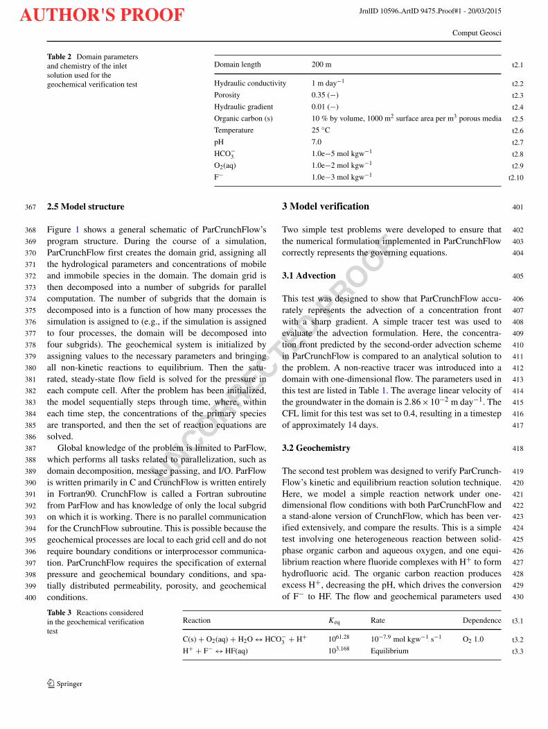
Figure 4 illustrates the strong parallel scaling perfor- 517

mance of this code. The measured relative speedup as 518

process count increases is nearly ideal from one to 125 519

processes (Fig. 4a). The solve time decreases significantly, 520

from 10.25 h with one process to 7.19 min with 125 pro- 521

cesses. Although the strong scaling displayed here is quite 522

good from one to 125 processes, it breaks down some- 523

where between 125 and 216 processes, which corresponds 524

to 69,000 and 40,000 dof per process, respectively (Fig. 4b). 525

This decrease in parallel performance can be attributed 526

to an increase in communication overhead as process count 527

increases; as pincreases, the domain is decomposed into an 528

increasing number of subgrid regions, the number of dof 529

per process decreases, and interprocessor communication 530

requirements increase. Strong parallel scaling performance 531

is not just a function of algorithmic or numerical or hard- 532

ware efficiency but also depends on the size of the problem 533

being simulated. The size of the problem used in this study 534

was chosen to avoid memory contention issues when the 535

process count was one, i.e., the problem size was based on 536

the resources available on BlueM. Had we chosen a base 537

process count larger than one, and used a problem of larger 538

size, we would see ideal strong scaling behavior at higher 539

process counts. Overall, ParCrunchFlow’s strong parallel 540

scaling is nearly ideal when the number of dof per process 541

is greater than 69,000, and illustrates the ability and limita- 542

tions of this code to decrease the time required to solve a 543

given problem by increasing the number of processors used. 544

4.2 Weak scaling 545

Weak parallel scaling is a measure of how the solution time 546

varies with the number of processes for a fixed problem 547

Table 5 Reactions consideredin the parallel scaling studies t5.1Reaction Keq Rate

t5.2C(s) + O2(aq) + H2O ↔ HCO−3 + H+ 1061.28 10−7.0 mol kgw−1 s−1

t5.3NO−3 + 2H+ + H2O ↔ NH+

4 + 2O2(aq) 10−41.27 Equilibrium

t5.4NH+4 ↔ NH3 + H+ 109.241 Equilibrium


UNCORRECTEDPROOF

Comput Geosci

Fig. 4 Time to solve versus process count in the strong scaling study (a) and relative strong parallel efficiency versus process count (b). Thenumber of degrees of freedom per process is plotted on the secondary axis

size per process. A unit problem of size n unknowns is548

simulated on one process, and both the problem size and549

number of processes are increased linearly. The number550

of unknowns per process stays constant. For weak parallel551

scaling, performance is represented by relative weak parallel552

efficiency:553

Eweak = T (n, 1)

T (np, p)(19)

where T is the simulation time as a function of problem size554

and process count, n is the problem size in unknowns, and555

p is the number of processes. For perfect parallel efficiency,556

the simulation time will remain constant, and Eweak = 1.557

The parameters used in the weak scaling study are listed558

in Table 6. The unit problem size was fixed at 500,000559

compute cells per process. Permeability is homogeneously560

distributed throughout the domain, and a hydraulic gradi-561

ent is present in the x-direction, producing one-dimensional562

flow in a three-dimensional domain. The geochemical sys-563

tem used here is the same as in the strong scaling study564

(Table 5), with five primary chemical species, two aqueous565

equilibrium reactions, and one kinetic heterogeneous reac- 566

tion, resulting in 2.5 million dof per process. The total 567

problem size was increased by distributing the unit prob- 568

lem in the y dimension proportionally to the number of 569

processes used, i.e., when the process count is one, the 570

dimensions of the domain are 50 m × 100 m × 100 m, 571

and when the process count is four, the dimensions of the 572

domain are 50 m × 400 m × 100 m. These simulations scale 573

up to 2048 cores, which equates to 1.024 billion compute 574

cells and 5.12 billion total dof. 575

The total wall clock time ranged from 1495 to 1885 s 576

for problem sizes ranging from 2.5 million total dof (p = 577

1) to 5.12 billion total dof (p = 2048) in the weak 578

parallel efficiency study (Fig. 5). Relative weak parallel effi- 579

ciency decreases as p increases, to a final value of 0.8 at 580

2048 cores. Weak parallel efficiency is nearly perfect up 581

to 16 processes. As the process count increases from 16 to 582

32, and the simulation requires the use of multiple com- 583

pute nodes, we observe a decrease in efficiency, which is 584

almost certainly a result of hardware inefficiencies as intern- 585

odal communication comes into play. All further decreases 586

Table 6 List of parametersused in the weak parallelscaling study

t6.1Hydraulic conductivity 0.5 m day−1


t6.3Hydraulic gradient (x-direction) 1.0 (−)

t6.4Unit problem size 50 m × 100 m × 100 m, discretized at 1 m

t6.5Simulation duration 50 days


UNCORRECTEDPROOF

Comput Geosci

Fig. 5 A plot of weak parallel scaling efficiency versus process count

in efficiency are most likely due to a mixture of hard-587

ware, numerical, and algorithmic inefficiencies. Overall, the588

weak scaling performance exhibited here is excellent, and589

the decrease in efficiency observed as the process count590

increases is very small considering the large number of pro-591

cesses and dof employed in this test. This test demonstrates592

ParCrunchFlow’s ability to represent large, field-scale sys-593

tems at reasonably high resolution, by leveraging massively594

parallel architecture. Although the maximum number of595

processes used in the weak scaling study was 2048, prior596

studies on the scalability of ParFlow [52, 53], which pro-597

vides the parallel framework for ParCrunchFlow, give rea-598

son to believe that ParCrunchFlow will scale relatively well599

up to 16,384 processes.600

5 Floodplain simulations601

ParCrunchFlow was used to conduct a series of simula-602

tions that investigate important interactions between bio-603

geochemical reactions and transport processes in subsurface604

systems. These simulations take place in a hypothetical605

floodplain aquifer with similarities to the U.S. Department606

of Energy-funded study site in Rifle, CO [55–57], and607

consider interactions between solid-phase organic carbon,608

aqueous oxygen, and nitrogen. Spatially variable nitrogen609

reduction has been observed at the Rifle site [58], pro-610

viding a good test case for the numerical simulation of a611

relevant problem. Three simulations were conducted with612

varying representations of physical and chemical hetero-613

geneity. Specifically, the distributions of saturated hydraulic614

and solid-phase organic carbon were varied between the 615

three simulations. Simulation 1 has constant permeability 616

throughout the domain, producing one-dimensional flow 617

conditions. Simulations 2 and 3 take place in a hetero- 618

geneous domain more representative of subsurface con- 619

ditions (Fig. 6) in a typical floodplain aquifer, where 620

higher-permeability alluvium is interspersed with lenses of 621

low-permeability channel deposits. The solid-phase organic 622

carbon is homogeneously distributed throughout the model 623

domain in simulations 1 and 2, and is only located in the 624

low-permeability lenses in simulation 3. The parameters 625

used in these simulations are summarized in Table 7. All 626

three simulations take place in a fully saturated, rectilinear 627

200 m × 200 m × 40 m domain, discretized at 1 m × 628

1 m × 0.1 m in the x, y, and z dimensions, respectively, 629

for a total of 16 million compute cells. The duration of these 630

simulations is 3600 days. 631

Although the distribution of solid-phase organic carbon 632

varies between simulations, the domain-averaged initial vol- 633

ume fraction is the same, 0.04(−), for all simulations. Sim- 634

ilarly for the permeability, the domain-averaged hydraulic 635

conductivity in all simulations is 0.852 m day−1. All other 636

parameters used in these simulations are constant between 637

simulations. The domain for simulations 2 and 3 (Fig. 6), 638

used to characterize the distribution of permeability and 639

solid-phase organic carbon in these simulations, was created 640

with the geostatistical software T-PROGS [59] and repre- 641

sents a realistic distribution of high- and low-permeability 642

zones in a typical floodplain aquifer. 643

The initial geochemical conditions and reactions con- 644

sidered here are listed in Tables 8 and 9, respectively. 645

A solution with 0.13 nmol kgw−1 aqueous oxygen and 646

1.0 mmol kgw−1 nitrate (inlet solution) is introduced into 647

the domain (floodplain condition) along the boundary at 648

x = 0 (northwest boundary in Fig. 7), where it gener- 649

ally flows in the positive x-direction (southeast boundary 650

in Fig. 7) and reacts with the solid-phase organic carbon, 651

which we model as an oxidative dissolution reaction using 652

Fig. 6 The model domain used in simulations 2 and 3. This domainrepresents a hypothetical floodplain aquifer, where red corresponds toareas of high permeability and blue represents low-permeability lenses


UNCORRECTEDPROOF

Comput Geosci

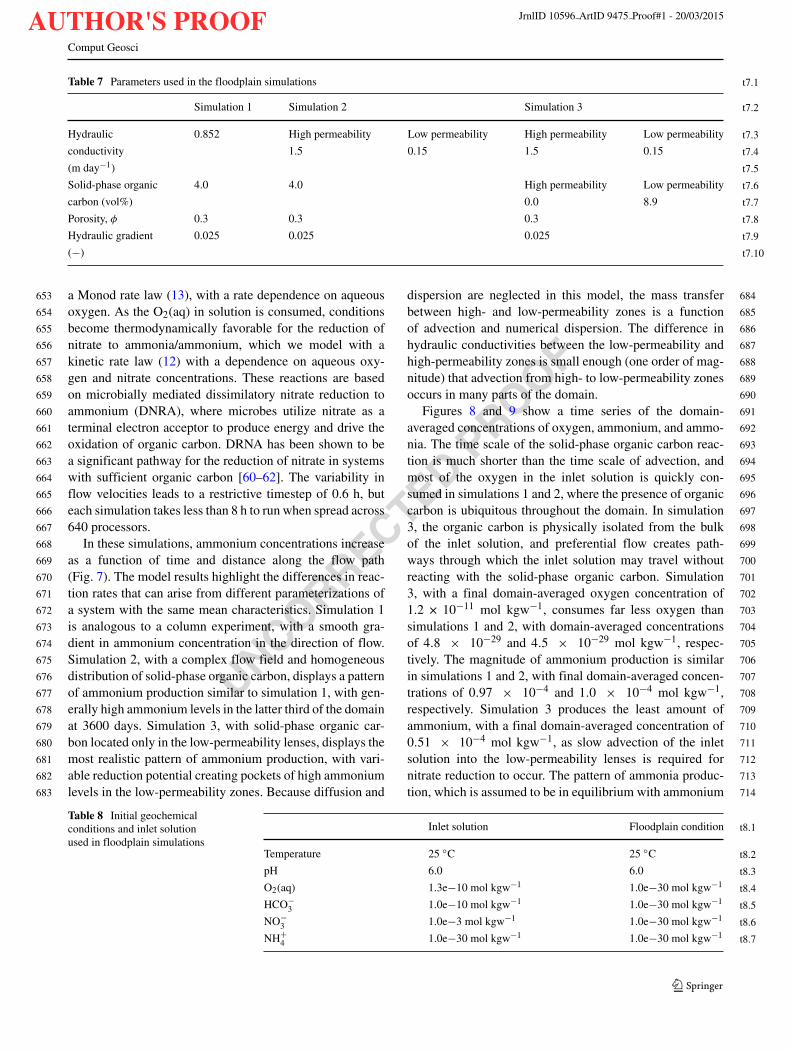
Table 7 Parameters used in the floodplain simulations t7.1

t7.2Simulation 1 Simulation 2 Simulation 3

t7.3Hydraulic 0.852 High permeability Low permeability High permeability Low permeability

t7.4conductivity 1.5 0.15 1.5 0.15

t7.5(m day−1)

t7.6Solid-phase organic 4.0 4.0 High permeability Low permeability

t7.7carbon (vol%) 0.0 8.9

t7.8Porosity, φ 0.3 0.3 0.3

t7.9Hydraulic gradient 0.025 0.025 0.025

t7.10(−)

a Monod rate law (13), with a rate dependence on aqueous653

oxygen. As the O2(aq) in solution is consumed, conditions654

become thermodynamically favorable for the reduction of655

nitrate to ammonia/ammonium, which we model with a656

kinetic rate law (12) with a dependence on aqueous oxy-657

gen and nitrate concentrations. These reactions are based658

on microbially mediated dissimilatory nitrate reduction to659

ammonium (DNRA), where microbes utilize nitrate as a660

terminal electron acceptor to produce energy and drive the661

oxidation of organic carbon. DRNA has been shown to be662

a significant pathway for the reduction of nitrate in systems663

with sufficient organic carbon [60–62]. The variability in664

flow velocities leads to a restrictive timestep of 0.6 h, but665

each simulation takes less than 8 h to run when spread across666

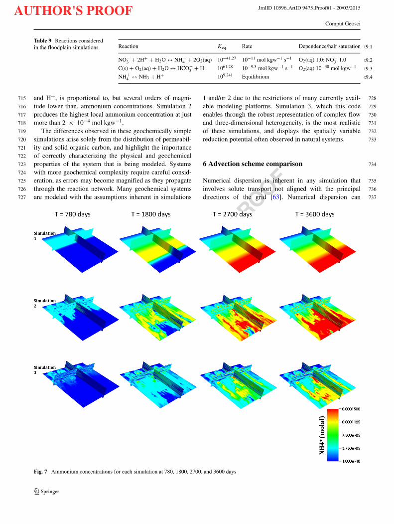
640 processors.667

In these simulations, ammonium concentrations increase668

as a function of time and distance along the flow path669

(Fig. 7). The model results highlight the differences in reac-670

tion rates that can arise from different parameterizations of671

a system with the same mean characteristics. Simulation 1672

is analogous to a column experiment, with a smooth gra-673

dient in ammonium concentration in the direction of flow.674

Simulation 2, with a complex flow field and homogeneous675

distribution of solid-phase organic carbon, displays a pattern676

of ammonium production similar to simulation 1, with gen-677

erally high ammonium levels in the latter third of the domain678

at 3600 days. Simulation 3, with solid-phase organic car-679

bon located only in the low-permeability lenses, displays the680

most realistic pattern of ammonium production, with vari-681

able reduction potential creating pockets of high ammonium682

levels in the low-permeability zones. Because diffusion and683

dispersion are neglected in this model, the mass transfer 684

between high- and low-permeability zones is a function 685

of advection and numerical dispersion. The difference in 686

hydraulic conductivities between the low-permeability and 687

high-permeability zones is small enough (one order of mag- 688

nitude) that advection from high- to low-permeability zones 689

occurs in many parts of the domain. 690

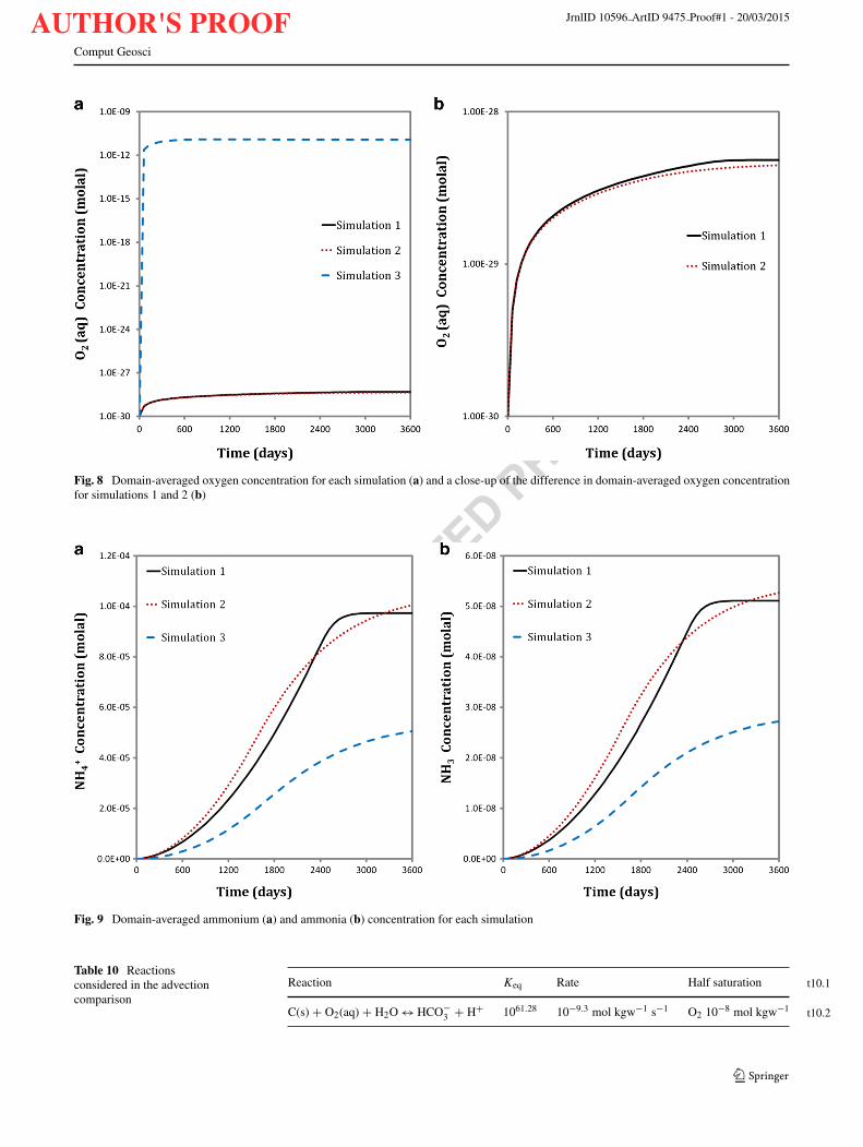
Figures 8 and 9 show a time series of the domain- 691

averaged concentrations of oxygen, ammonium, and ammo- 692

nia. The time scale of the solid-phase organic carbon reac- 693

tion is much shorter than the time scale of advection, and 694

most of the oxygen in the inlet solution is quickly con- 695

sumed in simulations 1 and 2, where the presence of organic 696

carbon is ubiquitous throughout the domain. In simulation 697

3, the organic carbon is physically isolated from the bulk 698

of the inlet solution, and preferential flow creates path- 699

ways through which the inlet solution may travel without 700

reacting with the solid-phase organic carbon. Simulation 701

3, with a final domain-averaged oxygen concentration of 702

1.2 × 10−11 mol kgw−1, consumes far less oxygen than 703

simulations 1 and 2, with domain-averaged concentrations 704

of 4.8 × 10−29 and 4.5 × 10−29 mol kgw−1, respec- 705

tively. The magnitude of ammonium production is similar 706

in simulations 1 and 2, with final domain-averaged concen- 707

trations of 0.97 × 10−4 and 1.0 × 10−4 mol kgw−1, 708

respectively. Simulation 3 produces the least amount of 709

ammonium, with a final domain-averaged concentration of 710

0.51 × 10−4 mol kgw−1, as slow advection of the inlet 711

solution into the low-permeability lenses is required for 712

nitrate reduction to occur. The pattern of ammonia produc- 713

tion, which is assumed to be in equilibrium with ammonium 714

Table 8 Initial geochemicalconditions and inlet solutionused in floodplain simulations

t8.1Inlet solution Floodplain condition

t8.2Temperature 25 ◦C 25 ◦C

t8.3pH 6.0 6.0

t8.4O2(aq) 1.3e−10 mol kgw−1 1.0e−30 mol kgw−1

t8.5HCO−3 1.0e−10 mol kgw−1 1.0e−30 mol kgw−1

t8.6NO−3 1.0e−3 mol kgw−1 1.0e−30 mol kgw−1

t8.7NH+4 1.0e−30 mol kgw−1 1.0e−30 mol kgw−1


UNCORRECTEDPROOF

Comput Geosci

Table 9 Reactions consideredin the floodplain simulations t9.1Reaction Keq Rate Dependence/half saturation

t9.2NO−3 + 2H+ + H2O ↔ NH+

4 + 2O2(aq) 10−41.27 10−11 mol kgw−1 s−1 O2(aq) 1.0; NO−3 1.0

t9.3C(s) + O2(aq) + H2O ↔ HCO−3 + H+ 1061.28 10−9.3 mol kgw−1 s−1 O2(aq) 10−30 mol kgw−1

t9.4NH+4 ↔ NH3 + H+ 109.241 Equilibrium

and H+, is proportional to, but several orders of magni-715

tude lower than, ammonium concentrations. Simulation 2716

produces the highest local ammonium concentration at just717

more than 2 × 10−4 mol kgw−1.718

The differences observed in these geochemically simple719

simulations arise solely from the distribution of permeabil-720

ity and solid organic carbon, and highlight the importance721

of correctly characterizing the physical and geochemical722

properties of the system that is being modeled. Systems723

with more geochemical complexity require careful consid-724

eration, as errors may become magnified as they propagate725

through the reaction network. Many geochemical systems726

are modeled with the assumptions inherent in simulations727

1 and/or 2 due to the restrictions of many currently avail- 728

able modeling platforms. Simulation 3, which this code 729

enables through the robust representation of complex flow 730

and three-dimensional heterogeneity, is the most realistic 731

of these simulations, and displays the spatially variable 732

reduction potential often observed in natural systems. 733

6 Advection scheme comparison 734

Numerical dispersion is inherent in any simulation that 735

involves solute transport not aligned with the principal 736

directions of the grid [63]. Numerical dispersion can 737

Fig. 7 Ammonium concentrations for each simulation at 780, 1800, 2700, and 3600 days


UNCORRECTEDPROOF

Comput Geosci

Fig. 8 Domain-averaged oxygen concentration for each simulation (a) and a close-up of the difference in domain-averaged oxygen concentrationfor simulations 1 and 2 (b)

Fig. 9 Domain-averaged ammonium (a) and ammonia (b) concentration for each simulation

Table 10 Reactionsconsidered in the advectioncomparison

t10.1Reaction Keq Rate Half saturation

t10.2C(s) + O2(aq) + H2O ↔ HCO−3 + H+ 1061.28 10−9.3 mol kgw−1 s−1 O2 10−8 mol kgw−1


UNCORRECTEDPROOF

Comput Geosci

Table 11 Parameters used forthe advection schemecomparison

t11.1High permeability Low permeability

t11.2Hydraulic conductivity 1.5 m day−1 0.05 m day−1

t11.3Solid-phase organic carbon 0 % by volume 10 % by volume



Table 12 Initial geochemicalconditions and inlet solutionused in the advectioncomparison

t12.1Inlet solution High permeability Low permeability

t12.2Temperature 25 ◦C 25 ◦C 25 ◦C

t12.3pH 6.0 6.0 6.0

t12.4O2(aq) 1.0e−6 mol kgw−1 1.0e−6 mol kgw−1 1.0e−30 mol kgw−1

t12.5HCO−3 1.0e−10 mol kgw−1 1.0e−10 mol kgw−1 1.0e−30 mol kgw−1

Fig. 10 A visual comparison of steady-state (T = 2280 days) oxygen concentrations for the first-order simulation (a) and the second-ordersimulation (b)

Fig. 11 Comparison of steady-state oxygen concentrations in a slice of the domain (z = 26 m) for the first-order simulation (a) and the second-order simulation (b)


UNCORRECTEDPROOF

Comput Geosci

influence concentration gradients and can have a significant738

impact on these large, field-scale reactive transport sim-739

ulations. The operator-splitting approach implemented in740

ParCrunchFlow provides the ability to use explicit advec-741

tion schemes, which can minimize numerical dispersion and742

more accurately represent systems with high degrees of het-743

erogeneity. Two simulations were conducted to quantify the744

effect that numerical dispersion can have on reaction rates745

in large, field-scale systems. These simulations are identi-746

cal aside from the advection scheme; one uses first-order747

upwinding and the other uses the second-order Godunov748

scheme. The same hypothetical floodplain domain that was749

used in the previous set of simulations (Fig. 6) is used750

here. The domain is constructed in a manner similar to751

simulation 3, with complex flow and solid-phase organic752

carbon located in the low-permeability zones. Here, we also753

model the biodegradation of solid organic carbon. This reac-754

tion (Table 10) is represented with a Monod rate law (13),755

in which reaction progress depends on the concentration of756

aqueous oxygen. The parameters and geochemical condi-757

tions used in these simulations are listed in Tables 11 and 12.758

The high-permeability zone of the domain was initialized759

with a solution identical to the inlet solution, to decrease the760

time required to reach steady-state conditions. The domain761

is 200 m × 200 m × 40 m, discretized at 1 m × 1 m × 0.1 m762

in the x, y, and z dimensions, respectively, for a total of 16763

million compute cells. The duration of these simulations is764

2280 days.765

The second-order scheme produces much sharper gradi-766

ents in aqueous oxygen concentrations and a more stratified767

system than the first-order scheme, where numerical dis-768

persion creates a smearing effect (Figs. 10 and 11). The769

first-order scheme results in more consumption of aqueous770

oxygen than the second-order scheme (Fig. 12). As the sim-771

ulation progresses, the discrepancy between the first- and772

second-order simulations increases. By the end of the sim-773

ulations, the domain-averaged oxygen concentration in the774

second-order case is 7.8 % larger than in the first-order775

case. Perhaps a better metric of the consumption of oxy-776

gen within the system is provided by an examination of the777

O2(aq) flux out of the domain (Fig. 13). Examining the out-778

going flux of aqueous oxygen allows an evaluation of the779

cumulative effects of numerical dispersion, after they have780

propagated through the length of the domain. The smooth781

gradients in solute concentration produced by the first-order782

scheme lead to a greater consumption, and lower outgoing783

flux of aqueous oxygen than do the sharp gradients pro-784

duced by the second-order scheme. The magnitude of the785

difference in steady-state oxygen flux is quite large; at a786

time of 2280 days, the second-order simulation produces787

a flux (0.0108 mol day−1) that is 25 % larger than the788

first-order flux (0.00865 mol day−1).789

Fig. 12 Domain-averaged oxygen concentrations for each simulation

The numerical dispersion produced by the first-order 790

scheme feeds back to the reaction rates as well. Figure 14 791

presents a comparison of the steady-state reaction rates in a 792

slice of the domain (z = 26 m), and Fig. 15 shows the distri- 793

bution of the non-zero reaction rates in each simulation. The 794

smooth gradients in oxygen concentrations produced with 795

Fig. 13 A semi-log plot of oxygen flux out of the domain for eachsimulation. The second-order flux is 25 % larger than the first-orderflux at late times


UNCORRECTEDPROOF

Comput Geosci

Fig. 14 Comparison of steady-state (T = 2280 days) reaction rates in a slice of the domain (z = 26 m) for the first-order simulation (a) and thesecond-order simulation (b)

the first-order scheme lead to a larger number of compute796

cells in which reaction progress occurs. These simulations797

contain approximately 7.2 million cells that contain solid798

organic carbon. At 2280 days, reactions occur in 58 % of799

those cells in the first-order simulation and 22 % of those800

cells in the second-order simulation. Although the number801

of cells in which reactions occur is almost three times higher802

in the first-order case, the distribution of rates in the second-803

order case is skewed toward larger values. The total amount804

of reaction represented by the distributions of rates shown 805

in Fig. 15 is similar, with less than a 2 % difference in the 806

total reaction occurring at 2280 days. This is evident when 807

examining a time series of domain-averaged reaction rates 808

(Fig. 16). 809

The differences observed in these simulations are entirely 810

due to the accuracy of the advection scheme. The smooth 811

gradients that the first-order scheme produces create an arti- 812

ficial mixing effect, which decreases the spatial variance 813

Fig. 15 The distribution of steady-state (T = 2280 days) reaction rates from the first-order (a) and second-order (b) simulations. The ratesshown here are rates of dissolution and are therefore positive. Only non-zero reaction rates are included


UNCORRECTEDPROOF

Comput Geosci

Fig. 16 The domain-averaged reaction rates for each simulation. Thereaction rates from the first-order case are slightly higher than those ofthe second-order case throughout the simulation

in concentrations and leads to an increase in overall reac-814

tion rates. The second-order scheme is less dispersive and815

produces localized zones of high reaction rates. The dif-816

ferences in domain-averaged reaction rates are small, but817

the cumulative effect, after propagating through the domain,818

results in a 25 % larger oxygen flux out of the system in the819

second-order simulation.820

These differences highlight the potential importance of821

using a higher-order advection scheme to represent field-822

scale systems. Increases in either the size of a simulation823

or the degree of the physical and/or chemical heterogeneity824

within a simulation may increase susceptibility to the neg-825

ative effects of numerical dispersion. As simulations grow826

larger, the error induced by numerical dispersion propa-827

gates through the domain, increasing with the length scale828

over which it operates. As the degree of heterogeneity829

increases, sharper gradients in solute concentrations arise,830

which lower-order schemes tend to smooth out. When simu-831

lating systems with both physical and chemical heterogene-832

ity, where many reactions tend to occur in small localized833

pockets, a higher-order advection scheme may be necessary834

to accurately represent the reaction dynamics.835

7 Discussion836

The transport scheme used here does not consider diffusion837

or dispersion terms. The authors feel that neglecting these838

terms is appropriate in some of the high Peclet number field-839

scale systems that this code was designed to represent. In840

these advection-dominated systems, the numerical disper- 841

sion inherent in the Eulerian discretization of the advection 842

equation will typically be of more consequence than the 843

physical processes themselves. However, numerical disper- 844

sion is grid size dependent, and oftentimes the grid size 845

cannot be tuned to provide the desired dispersive effect. For 846

certain problems, this is a shortcoming, and ParCrunchFlow 847

may provide a poor approximation of the system. To remedy 848

this situation, velocity-dependent physical dispersion will 849

be included in the next version of ParCrunchFlow. 850

ParCrunchFlow’s ability to finely resolve physical and 851

geochemical heterogeneities in large, field-scale systems 852

has implications for the numerical upscaling of effective 853

reaction rates in natural systems. The level of detail that can 854

be represented with this model allows us to explore the inter- 855

play between complex flow fields and variable distributions 856

of reactive solid phases in more detail than was previ- 857

ously possible. The minimal numerical dispersion produced 858

with the second-order advection scheme allows the repre- 859

sentation of sharp concentration gradients that result from 860

physical and geochemical heterogeneities, which provides 861

an opportunity to study reaction dynamics in a more realis- 862

tic numerical setting. The next iteration of ParCrunchFlow 863

will include a physically based linkage to surface flows, and 864

will be able to simulate areas of geochemical importance, 865

such as the hyporheic zone and the capillary fringe. 866

8 Conclusions 867

We have developed the parallel reactive transport code 868

ParCrunchFlow by coupling the parallel hydrologic code 869

ParFlow with the geochemical code CrunchFlow. Par- 870

CrunchFlow takes an operator-splitting approach to reac- 871

tive transport, where the reaction and transport terms are 872

decoupled and solved for separately. ParCrunchFlow allows 873

for numerical simulation of complex, heterogeneous sub- 874

surface environments where hydrological, chemical, and 875

microbial processes interact. The ability of this model to 876

represent sharp gradients in advancing concentration fronts 877

and solve systems with kinetically and thermodynamically 878

controlled reactions has been verified. ParCrunchFlow’s 879

excellent parallel scaling has been demonstrated, showing 880

that this platform is capable of representing highly resolved, 881

field-scale systems with a large number of unknowns. A 882

series of simulations involving the biologically mediated 883

reduction of nitrate in a floodplain aquifer were conducted. 884

These floodplain simulations show that this code enables 885

us to more realistically represent the variability in chem- 886

ical concentrations observed in many field-scale systems. 887

The numerical formulation implemented in ParCrunch- 888

Flow minimizes numerical dispersion and allows the use 889

of higher-order explicit advection schemes. The effects that 890


UNCORRECTEDPROOF

Comput Geosci

numerical dispersion can have on finely resolved, field-891

scale reactive transport simulations have been evaluated.892

The smooth gradients that the first-order scheme produces893

create an artificial mixing effect, which decreases the spatial894

variance in solute concentrations and leads to an increase895

in overall reaction rates. At the current time, we have896

completed enough of the model coupling to begin simula-897

tions. The development of ParCrunchFlow is ongoing, and898

the work presented here represents the first step toward899

creating a reactive transport model capable of simulat-900

ing the interactions that occur between complex, surface-901

subsurface flow and biogeochemical processes. Future902

work will include incorporating ParFlow’s transient, vari-903

ably saturated surface-subsurface flow solver, adding a904

capability to treat physical dispersion, including Crunch-905

Flow’s subroutines for ion exchange, surface complexation,906

and precipitation/dissolution-induced permeability-porosity907

feedbacks, and potentially coupling ParCrunchFlow to a908

land surface model (Common Land Model).909

Acknowledgments This material is based upon work supported as910part of the Subsurface Science Scientific Focus Area at Lawrence911Berkeley National Laboratory funded by the U.S. Department of912Energy, Office of Science, Office of Biological and Environmental913Research under Award Number DE-AC02-05CH11231.914

References915

1. Li, L., Peters, C.A., Celia, M.A.: Upscaling geochemical reac-916tion rates using pore-scale network modeling. Adv. Water Resour.91729(9), 1351–1370 (2006)918

2. White, A.F., Brantley, S.L.: The effect of time on the weathering of919silicate minerals: why do weathering rates differ in the laboratory920and field. Chem. Geol. 202(3), 479–506 (2003)921

3. Maher, K., Steefel, C.I., DePaolo, D.J., Viani, B.E.: The mineral922dissolution rate conundrum: insights from reactive transport mod-923eling of U isotopes and pore fluid chemistry in marine sediments.924Geochim. Cosmochim. Acta. 70(2), 337–363 (2006)925

4. Navarre-Sitchler, A., Brantley, S.: Basalt weathering across scales.926Earth Planet. Sci. Lett. 261(1), 321–334 (2007)927

5. Lichtner, P.C.: Continuum model for simultaneous chemical reac-928tions and mass transport in hydrothermal systems. Geochim.929Cosmochim. Acta. 49(3), 779–800 (1985)930

6. Steefel, C.I., Lasaga, A.C.: A coupled model for transport of mul-931tiple chemical species and kinetic precipitation/dissolution reac-932tions with application to reactive flow in single phase hydrother-933mal systems. Am. J. Sci. 294(5), 529–592 (1994)934

7. Steefel, C.I., DePaolo, D.J., Lichtner, P.C.: Reactive transport935modeling: an essential tool and a new research approach for the936Earth sciences. Earth. Planet. Sci. Lett. 240(3), 539–558 (2005)937

8. Dagan, G.: Statistical theory of groundwater flow and transport:938pore to laboratory, laboratory to formation, and formation to939regional scale. Water Resour. Res. 22(9S), 120S–134S (1986)940

9. Dagan, G.: The significance of heterogeneity of evolving scales to941transport in porous formations. Water Resour. Res. 30(12), 3327–9423336 (1994)943

10. Cushman, J.H.: Dynamics of Fluids in Hierarchical Porous Media.944Academic Press Inc. Ltd., London (1990)945

11. Gutierrez, J.L., Jones, C.G.: Physical ecosystem engineers as 946agents of biogeochemical heterogeneity. Bioscience 56(3), 227– 947236 (2006) 948

12. Zhou, J., Xia, B., Huang, H., Palumbo, A.V., Tiedje, J.M.: Micro- 949bial diversity and heterogeneity in sandy subsurface soils. Appl. 950Environ. Microbiol. 70(3), 1723–1734 (2004) 951

13. Englert, A., Hubbard, S., Williams, K., Li, L., Steefel, C.: Feed- 952backs between hydrological heterogeneity and bioremediation 953induced biogeochemical transformations. Environ. Sci. Technol. 95443(14), 5197–5204 (2009) 955

14. Neuman, S.P., Zhang, Y.K.: A quasi-linear theory of non-Fickian 956and Fickian subsurface dispersion: 1. Theoretical analysis with 957application to isotropic media. Water Resour. Res. 26(5), 887–902 958(1990) 959

15. Li, L., Steefel, C.I., Yang, L.: Scale dependence of mineral 960dissolution rates within single pores and fractures. Geochim. 961Cosmochim. Acta. 72(2), 360–377 (2008) 962

16. Navarre-Sitchler, A., Steefel, C.I., Yang, L., Tomutsa, L., Brantley, 963S.L.: Evolution of porosity and diffusivity associated with chem- 964ical weathering of a basalt clast. J. Geophys. Res. (Earth Surf.) 965114(F2) (2009) 966

17. Yabusaki, S.B., Steefel, C.I., Wood, B.: Multidimensional, multi- 967component, subsurface reactive transport in nonuniform velocity 968fields: code verification using an advective reactive streamtube 969approach. J. Contam. Hydrol. 30(3), 299–331 (1998) 970

18. Steefel, C.I.: New directions in hydrogeochemical transport mod- 971eling: incorporating multiple kinetic and equilibrium reaction 972pathways. In: Lawrence Livermore National Lab., CA (US) 973(2000) 974

19. Velbel, M.A.: Constancy of silicate-mineral weathering-rate ratios 975between natural and experimental weathering: implications for 976hydrologic control of differences in absolute rates. Chem. Geol. 977105(1), 89–99 (1993) 978

20. Clow, D., Drever, J.: Weathering rates as a function of flow 979through an alpine soil. Chem. Geol. 132(1), 131–141 (1996) 980

21. Maher, K.: The dependence of chemical weathering rates on fluid 981residence time. Earth Planet. Sci. Lett. 294(1), 101–110 (2010) 982

22. Navarre-Sitchler, A., Steefel, C.I., Sak, P.B., Brantley, S.L.: A 983reactive-transport model for weathering rind formation on basalt. 984Geochim. Cosmochim. Acta. 75(23), 7644–7667 (2011) 985

23. Siirila, E.R., Maxwell, R.M.: Evaluating effective reaction rates 986of kinetically driven solutes in large-scale, statistically anisotropic 987media: human health risk implications. Water Resour. Res. 48(4) 988(2012) 989

24. Frei, S., Fleckenstein, J., Kollet, S., Maxwell, R.: Patterns and 990dynamics of river–aquifer exchange with variably-saturated flow 991using a fully-coupled model. J. Hydrology 375(3), 383–393 992(2009) 993

25. Maxwell, R.M., Kollet, S.J.: Quantifying the effects of three- 994dimensional subsurface heterogeneity on Hortonian runoff pro- 995cesses using a coupled numerical, stochastic approach. Adv. Water 996Resour. 31(5), 807–817 (2008) 997

26. Ashby, S.F., Falgout, R.D.: A parallel multigrid preconditioned 998conjugate gradient algorithm for groundwater flow simulations. 999Nucl. Sci. Eng. 124(1), 145–159 (1996) 1000

27. Jones, J.E., Woodward, C.S.: Newton–Krylov-multigrid solvers 1001for large-scale, highly heterogeneous, variably saturated flow 1002problems. Adv. Water Resour. 24(7), 763–774 (2001) 1003

28. Kollet, S.J., Maxwell, R.M.: Integrated surface–groundwater flow 1004modeling: a free-surface overland flow boundary condition in a 1005parallel groundwater flow model. Adv. Water Resour. 29(7), 945– 1006958 (2006) 1007

29. Bell, J.B., Dawson, C.N., Shubin, G.R.: An unsplit, higher order 1008Godunov method for scalar conservation laws in multiple dimen- 1009sions. J. Comput. Phys. 74(1), 1–24 (1988) 1010


UNCORRECTEDPROOF

Comput Geosci

30. Steefel, C., Yabusaki, S.: OS3D/GIMRT, software for1011multicomponent-multidimensional reactive transport. User man-1012ual and programmer’s guide, PNL-11166. Pacific Northwest1013National Laboratory, Richland, WA 99352 (1996)1014

31. Steefel, C.I., Appelo, C.A.J., Arora, B., Jacques, D., Kalbacher, T.,1015Kolditz, O., Lagneau, V., Lichtner, P.C., Mayer, K.U., Meeussen,1016J.C.L., Molins, S., Moulton, D., Parkhurst, D.L., Shao, H.,1017Simunek, J., Spycher, N., Yabusaki, S.B., Yeh, G.T.: Reactive1018transport codes for subsurface environmental simulation. Submit-1019ted to Computational Geosciences (Submitted 2014)1020

32. Maher, K., Steefel, C.I., White, A.F., Stonestrom, D.A.: The role1021of reaction affinity and secondary minerals in regulating chemical1022weathering rates at the Santa Cruz Soil Chronosequence, Califor-1023nia. Geochim. Cosmochim. Acta. 73(10), 2804–2831 (2009)1024

33. Atchley, A.L., Maxwell, R.M., Navarre-Sitchler, A.K.: Using1025streamlines to simulate stochastic reactive transport in hetero-1026geneous aquifers: kinetic metal release and transport in CO21027impacted drinking water aquifers. Adv. Water Resour. 52, 93–1061028(2013)1029

34. Chang, H.-s., Um, W., Rod, K., Serne, R.J., Thompson, A., Per-1030drial, N., Steefel, C.I., Chorover, J.: Strontium and cesium release1031mechanisms during unsaturated flow through waste-weathered1032Hanford sediments. Environ. Sci. Technol. 45(20), 8313–83201033(2011)1034

35. Wanner, C., Eggenberger, U., Mader, U.: A chromate-1035contaminated site in southern Switzerland–part 2: reactive1036transport modeling to optimize remediation options. Appl.1037Geochem. 27(3), 655–662 (2012)1038

36. Yeh, G., Tripathi, V.: A critical evaluation of recent developments1039in hydrogeochemical transport models of reactive multichemical1040components. Water Resour. Res. 25(1), 93–108 (1989)1041

37. Walter, A., Frind, E., Blowes, D., Ptacek, C., Molson, J.: Modeling1042of multicomponent reactive transport in groundwater: 1. Model1043development and evaluation. Water Resour. Res. 30(11), 3137–10443148 (1994)1045

38. Steefel, C.I., MacQuarrie, K.T.: Approaches to modeling of reac-1046tive transport in porous media. Rev. Mineral. Geochem. 34(1), 85–1047129 (1996)1048

39. Maxwell, R., Putti, M., Meyerhoff, S., Delfs, J.-O., Ferguson, I.,1049Ivanov, V., Kim, J., Kolditz, O., Kollet, S., Kumar, M., Lopez,1050S., Niu, J., Paniconi, C., Park, Y.-J., Phanikumar, M., Shen, C.,1051Sudicky, E., Sulis, M.: Surface-subsurface model intercompari-1052son: a first set of benchmark results to diagnose integrated hydrol-1053ogy and feedbacks. Water Resour. Res. 50, 1531–1549 (2014).1054doi:10.1002/2013WR0137251055

40. Reed, M.H.: Calculation of multicomponent chemical equilibria1056and reaction processes in systems involving minerals, gases and1057an aqueous phase. Geochim. Cosmochim. Acta 46(4), 513–5281058(1982)1059

41. Kirkner, D.J., Reeves, H.: Multicomponent mass transport with1060homogeneous and heterogeneous chemical reactions: effect of the1061chemistry on the choice of numerical algorithm: 1. Theory. Water1062Resour. Res. 24(10), 1719–1729 (1988)1063

42. Lasaga, A.C.: Rate laws of chemical reactions. Rev. Mineralology1064Geochemistry 8 (1981)1065

43. Lasaga, A.C.: Chemical kinetics of water-rock interactions. J.1066Geophys. Res. (Solid Earth) 89(B6), 4009–4025 (1984)1067

44. Aagaard, P., Helgeson, H.C.: Thermodynamic and kinetic con-1068straints on reaction rates among minerals and aqueous solutions;1069I, theoretical considerations. Am. J. Sci. 282(3), 237–285 (1982)1070

45. Strang, G.: On the construction and comparison of difference1071schemes. SIAM J. Numer. Anal. 5(3), 506–517 (1968)1072

46. Valocchi, A.J., Malmstead, M.: Accuracy of operator splitting1073for advection-dispersion-reaction problems. Water Resour. Res.107428(5), 1471–1476 (1992)1075

47. Kanney, J.F., Miller, C.T., Kelley, C.: Convergence of itera- 1076tive split-operator approaches for approximating nonlinear reac- 1077tive transport problems. Adv. Water Resour. 26(3), 247–261 1078(2003) 1079

48. Navarre-Sitchler, A.K., Maxwell, R.M., Siirila, E.R., Hammond, 1080G.E., Lichtner, P.C.: Elucidating geochemical response of shal- 1081low heterogeneous aquifers to CO< sub> 2< / sub> leakage 1082using high-performance computing: implications for monitoring 1083of CO<sub> 2< /sub> sequestration. Adv. Water Resour. 53, 108445–55 (2013) 1085

49. Hammond, G., Lichtner, P., Mills, R.: Evaluating the performance 1086of parallel subsurface simulators: an illustrative example with 1087PFLOTRAN. Water Resour. Res. (2014) 1088

50. Hammond, G.E., Lichtner, P.C.: Field-scale model for the nat- 1089ural attenuation of uranium at the Hanford 300 Area using 1090high-performance computing. Water Resour. Res. 46(9) (2010) 1091

51. Hammond, G., Lichtner, P., Lu, C.: Subsurface multiphase flow 1092and multicomponent reactive transport modeling using high- 1093performance computing. In: Journal of Physics: Conference Series 10942007, vol. 1, p. 012025. IOP Publishing 1095

52. Kollet, S.J., Maxwell, R.M., Woodward, C.S., Smith, S., Van- 1096derborght, J., Vereecken, H., Simmer, C.: Proof of concept of 1097regional scale hydrologic simulations at hydrologic resolution uti- 1098lizing massively parallel computer resources. Water Resour. Res. 109946(4) (2010) 1100

53. Maxwell, R.M.: A terrain-following grid transform and precon- 1101ditioner for parallel, large-scale, integrated hydrologic modeling. 1102Adv. Water Resour. 53, 109–117 (2013) 1103

54. Knoll, D.A., Keyes, D.E.: Jacobian-free Newton–Krylov methods: 1104a survey of approaches and applications. J. Comput. Phys. 193(2), 1105357–397 (2004) 1106

55. Li, L., Steefel, C.I., Kowalsky, M.B., Englert, A., Hubbard, S.S.: 1107Effects of physical and geochemical heterogeneities on mineral 1108transformation and biomass accumulation during biostimulation 1109experiments at Rifle, Colorado. J. Contam. Hydrol. 112(1), 45–63 1110(2010) 1111

56. Hyun, S.P., Fox, P.M., Davis, J.A., Campbell, K.M., Hayes, K.F., 1112Long, P.E.: Surface complexation modeling of U (VI) adsorption 1113by aquifer sediments from a former mill tailings site at Rifle, 1114Colorado. Environ. Sci. Technol. 43(24), 9368–9373 (2009) 1115

57. N’Guessan, A.L., Vrionis, H.A., Resch, C.T., Long, P.E., Lovley, 1116D.R.: Sustained removal of uranium from contaminated ground- 1117water following stimulation of dissimilatory metal reduction. 1118Environ. Sci. Technol. 42(8), 2999–3004 (2008) 1119

58. Mouser, P.J., N’Guessan, A.L., Elifantz, H., Holmes, D.E., 1120Williams, K.H., Wilkins, M.J., Long, P.E., Lovley, D.R.: Influence 1121of heterogeneous ammonium availability on bacterial community 1122structure and the expression of nitrogen fixation and ammo- 1123nium transporter genes during in situ bioremediation of uranium- 1124contaminated groundwater. Environ. Sci. Technol. 43(12), 4386– 11254392 (2009) 1126

59. Carle, S.F.: T-PROGS: Transition probability geostatistical soft- 1127ware. University of California, Davis (1999) 1128

60. Smith, M.S.: Dissimilatory reduction of NO2- to NH4+ and N2O 1129by a soil Citrobacter sp. Appl. Environ. Microbiol. 43(4), 854–860 1130(1982) 1131

61. Caskey, W.H., Tiedje, J.M.: Evidence for clostridia as agents of 1132dissimilatory reduction of nitrate to ammonium in soils. Soil Sci. 1133Soc. Am. J. 43(5), 931–936 (1979) 1134

62. Kaspar, H.F., Tiedje, J.M., Firestone, R.B.: Denitrification and dis- 1135similatory nitrate reduction to ammonium in digested sludge. Can. 1136J. Microbiol. 27(9), 878–885 (1981) 1137

63. Cirpka, O.A., Frind, E.O., Helmig, R.: Numerical simulation 1138of biodegradation controlled by transverse mixing. J. Contam. 1139Hydrol. 40(2), 159–182 (1999) 1140

ParCrunchFlow: an efficient, parallel reactive transport...

Documents

Transcript of ParCrunchFlow: an efficient, parallel reactive transport...