Parametrized Complexity of Virtual Network Embeddings ... · Parametrized Complexity of Virtual...

Public Review for

Parametrized Complexity of VirtualNetwork Embeddings: Dynamic & Linear

Programming ApproximationsM. Rost, E. Dohne, S. Schmid

Network virtualization requires e�cient mapping of virtual networks onto

the physical network. Unfortunately, this problem is NP-complete, and solv-

ing it approximately also poses serious computational challenges. Existing

solutions tend to be heuristics that do not provide formal performance guar-

antees.

Matthias Rost, Elias Dohne, and Stefan Schmid explore a parameterized-

complexity approach and first consider the Valid Mapping Problem (VMP)

that asks for a valid minimal-cost mapping of a virtual network onto the phys-

ical network. Specifically, the authors consider the virtual-network treewidth

as a parameter that captures closeness of the virtual-network graph to a tree.

While virtual networks typically have bounded treewidth, the paper develops

a DynVMP algorithm that decomposes the virtual-network graph into trees

and applies dynamic programming to solve VMP starting from the leaves

of the tree decomposition. The computational complexity of the solution

belongs to the XP class, and DynVMP runs in polynomial time for virtual

networks with bounded treewidth. Then, using a Fully Polynomial-Time Ap-

proximation Scheme (FPTAS) for minimum-cost Latency-Constrained Short-

est Paths (LCSP), the paper adapts DynVMP to support latency constraints.

Based on their successful solution for VMP, the authors tackle the Virtual

Network Embedding Problem (VNEP) where the virtual-network mapping

should be not only valid but also feasible with respect to capacity con-

straints. In particular, Rost, Dohne, and Schmid extend their previous

column-generation linear-programming approximation for the o✏ine VNEP

and generalize the solution for an arbitrary virtual-network graph. Again, the

proposed solution runs in polynomial time for virtual networks with bounded

treewidth and is adapted to accommodate latency constraints.

Supplementing the theoretical results on achieved runtime and solution-

quality guarantees, the paper experimentally evaluates its approach against

existing heuristics. First, the evaluation assesses the treewidth of random

graphs and shows that their tree decomposition can be done on the order

of seconds. Then, the paper examines the runtime and performance of its

solution for the o✏ine VNEP with four ViNE-heuristic variants.

Public review written bySergey Gorinsky

IMDEA Networks Institute, Spain

ACM SIGCOMM Computer Communication Review Volume 49 Issue 1, January 2019

Parametrized Complexity of Virtual Network Embeddings:Dynamic & Linear Programming ApproximationsMatthias Rost

TU Berlin, [email protected]

Elias DöhneTU Berlin, Germany

[email protected]

Stefan SchmidUniversity of Vienna, [email protected]

ABSTRACTThis paper makes the case for a parametrized complexity approachto tackle the fundamental but notoriously hard Virtual NetworkEmbedding Problem. In particular, we show that the structure ofthe to-be-embedded virtual network requests can be exploited to-ward fast (i.e.,fixed-parameter tractable) approximation algorithms,using dynamic as well as linear programming algorithms.

Our approach does provide formal guarantees on the runtimeand solution quality and can safeguard also latency constraints.Using extensive computational experiments we demonstrate thepractical relevance of our novel approach.

CCS CONCEPTS•Networks→Network resources allocation; •Theory of com-putation → Fixed parameter tractability;

KEYWORDSVirtual Network Embedding, Approximation, Fixed-ParameterTractability, Dynamic Programming, Linear Programming

1 INTRODUCTIONThe Virtual Network Embedding Problem (VNEP) captures theessence of many resource allocation problems in networks [5]:Given are a substrate network, representing the physical infras-tructure, and a virtual request graph, representing a customer’sworkload; the task is to map each virtual request node to a phys-ical substrate node and to realize each virtual request edge as apath in the substrate connecting the respective servers while safe-guarding, among others, capacity constraints. The VNEP has at-tracted much interest over the last years and is closely related toother embedding problems, e.g., the embedding of service functionchains [8], virtual clusters [1], or virtual datacenters [13]. Indeed,in all of these cases a request topology is to be embedded in theprovider’s physical substrate network. Figure 1 gives an example.

Alas, the VNEP is algorithmically very challenging: it isNP-complete and inapproximable under any objective [10]. Evenmore, the VNEP remains NP-complete in the absence of capac-ity constraints. Concretely, given restrictions on the mapping ofrequest nodes and edges, the respective Valid Mapping Problem(VMP) asking to determine a valid mapping respecting only thegiven restrictions, is NP-complete, even for planar and degree-bounded request graphs. However, the VMP is not only an elemen-tary problem, solving the VMP was recently also shown to be ofcrucial importance for the development of approximations for theVNEP: to approximate the offline variant of the VNEP using ran-domized rounding the computation of (convex combinations of)valid mappings using Linear Programming (LP) is necessary [11].

A B

CD

AC B

D

1

11

1

6

Request Graph Gr

Embedding 1/2

1/2 1/2

1/2

2/3

1/3

1 4

3 1

2/2 4/5

0/0 1/13/3

Substrate Network GS

Figure 1: Exemplary embedding of a request on a substrate.The numbers represent demands and allocations/capacities.

Contributions. This paper initiates the study of a parametrizedcomplexity approach to solve the fundamental Valid MappingProblem, which in turn leads to novel solutions for the VNEP.The motivation behind a parametrized complexity approach isthat many NP-hard problems become polynomial-time tractablewhen considering input parameters beyond the input size: theparametrized complexity classes F PT and XP contain prob-lems that can be solved in time O (2poly(k ) · poly( |X |)) andO ( |X |poly(k ) + poly( |X |)) for a problem instanceX with parameterk , respectively [6]. We employ the treewidth of the request graphas parametrization, which measures the closeness of the requestgraph to a tree [2] and derive a number of new results:(1) We develop the dynamic programming algorithm

DynVMP to solve the VMP, which runs in XP-timeO (npoly(k )S · poly(nS · nr )), where nS and nr denote thenumber of substrate and request nodes, respectively, and kdenotes the treewidth of the request graph. Thus, for graphsof bounded treewidth DynVMP runs in polynomial-time.

(2) Based on Linear Programming duality, we show that theDynVMP algorithm can be used as separation oracle and de-rive an efficient column generation approach for solving LinearProgramming relaxations of the VNEP. Accordingly, the previ-ous (polynomial-time) approximation result of [11] for cactusgraphs is generalized to graphs of bounded treewidth, whileyielding XP-approximations for all other graph classes.

(3) For the VNEP with per-edge latency constraints, we derive anovel approximation result based on computing approximatelatency-observing mappings using the DynVMP algorithm.

(4) To demonstrate the applicability of our approach in practice,we study the treewidth of random graphs, and evaluate ran-domized rounding heuristics with state-of-the-art heuristics.

Novelty & RelatedWork. TheVNEP has receivedmuch attentionover the last years and we refer to the survey [5] for an overview.Most existing works consider heuristics which do not provide anyformal performance guarantees.

Much less is known about polynomial-time approximation al-gorithms. Even et al. [4] present an approximation algorithm forlinear chain requests. A first more general approximation of the


offline VNEP (cf. Definition 2.5) was recently proven for the classof cactus request graphs [11], i.e. graphs in which cycles intersectin at most a single node. In particular, it was shown that the pre-viously known Multi-Commodity Flow (MCF) LP formulation [3]yields invalid mappings. Hence, the integrality gap of the MCF for-mulation is unbounded, rendering it useless for approximations.Accordingly, a novel LP formulation was proposed which alwaysreturns valid mappings, but grows in size compared to the MCF LP.

In this paper, we present a parametrized column genera-tion approach to compute optimal LP solutions for arbitrary re-quest graphs based on dynamic programming. Leveraging thisparametrized complexity perspective, we not only generalize thepreviously known approximation to arbitrary graphs, but also ob-tain approximations for the VNEP under latency constraints. Weare not aware of any VNEP approximations respecting latencies.

Structure. Section 2 introduces our formal model, and Section 3presents the idea of decomposing requests into trees. Our dynamicprogram is given in Section 4 and our approximations in Section 5.In Section 6 rounding heuristics are discussed. Our evaluation ispresented in Section 7. We conclude our work in Section 8.2 FORMAL MODELWithin this section theVNEP and theVMP are formally introduced.As latency constraints play an important role in Service FunctionChaining [8], we (optionally) incorporate these here.

Substrate Network. We refer to the physical network as sub-strate network and model it as directed graph GS = (VS ,ES ). Ca-pacities of the substrate are given via the function dS : GS → R≥0.The capacity dS (u) of node u ∈ VS may represent the number of(virtual) CPUs while the capacity dS (u,v ) of edge (u,v ) ∈ ES rep-resents the available bandwidth.We denote byPS the set of all sim-ple paths in GS . Each substrate element x ∈ GS may be attributedwith costs cS (x ) ∈ R≥0 for using it (per unit capacity). Substrateedges may be attributed with latencies via lS : ES → R≥0.

Request Graphs. A request is similarly modeled as di-rected graph Gr = (Vr ,Er ) together with node and edge de-mands dr : Gr → R≥0. Per edge latency bounds are given bylr : Er → R≥0, when latencies are considered. Each request r ∈ Rmay be attributed with a profit br ∈ R≥0 that the provider obtainswhen embedding the request, subject to the following restrictions.

Mapping Restrictions. Virtual nodes and edges can only bemapped on substrate nodes and edges of sufficient capacity. Fur-thermore, the customer or provider may restrict the mapping ofrequest nodes i ∈ Vr and edges (i, j ) ∈ Er by providing sets offorbidden substrate nodes V i

S ⊆ VS and edges Ei, jS ⊆ ES . The

set V iS may for example include substrate nodes too distant to

the customer or servers not suited to host the functionality of re-quest node i . Similarly, the set Ei, jS contains edges which mustbe avoided due to security or other technical policies. Accord-ingly, we denote the set of suitable substrate nodes for i ∈ Vr byV r,iS = {u ∈ VS \ V

iS | dS (u) ≥ dr (i )} while the set of suitable

substrate edges for (i, j ) ∈ Er is denoted by Er,i, jS = {(u,v ) ∈ES \ E

i, jS | dS (u,v ) ≥ dr (i, j )}. The maximal demand dmax (r ,x ) of

any request element for a single substrate resource x ∈ GS is de-fined as dmax (r ,u) = max({0} ∪ {dr (i ) | i ∈ Vr : u ∈ V r,i

S }) and

dmax (r ,u,v ) = max({0} ∪ {dr (i, j ) | (i, j ) ∈ Er : (u,v ) ∈ Er,i, jS }) forsubstrate nodes u ∈ VS and edges (u,v ) ∈ ES , respectively.

Problem Definitions. According to the above introduction ofmapping restrictions, a valid mapping is defined as follows.

Definition 2.1 (Valid Mapping). A valid mapping of request r ∈R to the substrate GS is a tuple mr = (mV

r ,mEr ) of functions that

map nodes and edges, respectively, s.t. the following holds:• The function mV

r : Vr → VS maps virtual nodes validly to sub-strate nodes, such thatmV

r (i ) ∈ V r,iS holds for i ∈ Vr .

• The function mEr : Er → PS maps virtual edges (i, j ) ∈ Er to

valid simple paths in GS connecting mVr (i ) to mV

r (j ), such thatmEr (i, j ) ⊆ Er,i, jS holds for (i, j ) ∈ Er .

• When latencies are considered !(u,v )∈mE

r (i, j ) lS (u,v ) ≤ lr (i, j )must hold for (i, j ) ∈ Er .

The set of all valid mappings of request r is denoted byMr . !Hence, a valid mapping enforces the validity of each single vir-

tual element with respect to mapping restrictions and resource ca-pacities. Cumulative resource allocations are defined as follows:

Definition 2.2 (Allocations). We denote by A(mr ,x ) ∈ R≥0 theresource allocation induced by the valid mapping mr = (mV

r ,mEr )

on substrate element x ∈ GS . For u ∈ VS and (u,v ) ∈ ES thefollowing holds, respectively: A(mr ,u) =

!i ∈Vr :mV

r (i )=u dr (i ) andA(mr ,u,v ) =

!(i, j )∈Er :(u,v )∈mE

r (i, j ) dr (i, j ). We denote the maxi-mal allocation that a valid mapping may impose on a substrateresource x ∈ GS by Amax (r ,x ) = maxmr ∈Mr A(mr ,x ) . !

A set of mappings is feasible if it respects resource capacities:

Definition 2.3 (Feasible Embedding). A set of mappings {mr }r ∈Rover a set of requests R is feasible, if and only if !r ∈R A(mr ,x ) ≤dS (x ) holds for x ∈ GS . A single mapping mr is feasible, if thisholds for the singleton set {mr }. !

The online and offline VNEP are defined as follows:

Definition 2.4 (Online Virtual Network Embedding Problem). Theonline VNEP asks for a feasible embeddingmr of a single requestr minimizing the cost c (mr ) =

!x ∈GS cS (x ) · A(mr ,x ). !

Definition 2.5 (Offline Virtual Network Embedding Problem). Theoffline VNEP asks for a feasible embedding {mr }r ∈R′ of a subsetof requests R ′ ⊆ R maximizing the profit !r ∈R′ br . !

As the feasibility of an embedding implies the validity of therespective mappings, the computation of valid mappings is a pre-requisite for both VNEP variants. We also introduce the (online)Valid Mapping Problem as follows:

Definition 2.6 (Valid Mapping Problem (VMP)). Given a request r ,theVMP asks for finding the validmappingmr minimizing the costfunction c (mr ) =

!x ∈GS cS (x ) · A(mr ,x ). !

We note that when request demands are small compared to thesubstrate capacities, the online VNEP reduces to the VMP:

Observation 2.7. Given a request for which any valid mappingmr ∈ Mr is feasible, i.e. Amax (r ,x ) ≤ dS (x ) holds for all substrateresources x ∈ GS , then the online VNEP reduces to the VMP: an opti-mal solution to the VMP is an optimal solution to the VNEP.


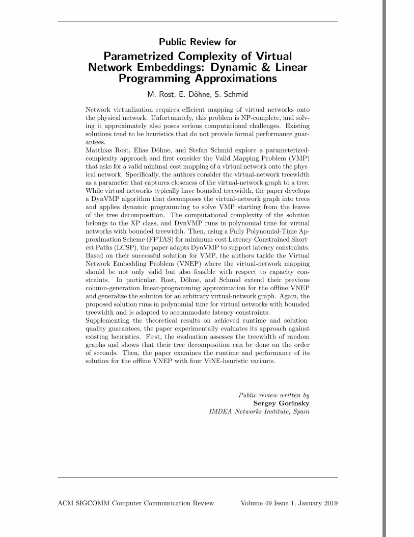
3 REQUEST GRAPH TREE DECOMPOSITIONSIn the following, we revisit the notion of tree decompositions [2, 6]and apply it to request graphs. Tree decompositions are used to rep-resent arbitrary graphs as trees (cf. Figure 2). The definition of treedecompositions ensures that (i) all nodes and edges of the requestgraph are covered while (ii) preserving crucial structural informa-tion of the original graph. Combinatorial optimization problems asthe VMP can then be solved on this tree representation by usingdynamic programming [6]. As tree decompositions are defined forundirected graphs, we consider undirected request graphs:

Definition 3.1 (Undirected Request Graph Gr ). For a requestgraph Gr = (Vr ,Er ) its undirected interpretation Gr = (Vr ,Er ) isgiven by Er = {{i, j}|(i, j ) ∈ Er } on the original node set Vr . !

Note that directed, antiparallel edges (i, j ), (j, i ) ∈ Er of the orig-inal request graph are accordingly represented using only a singleundirected edge {i, j} ∈ Er . Tree decompositions, here concerningthe request graphs, are then defined as follows [6].

Definition 3.2 (Tree Decomposition Tr = (Tr ,Br )). Given anundirected request Gr = (Vr ,Er ), a tree decomposition of Gr isa pair Tr = (Tr ,Br ) consisting of an undirected treeTr = (VT ,ET )and a family Br = {Bt }t ∈VT of subsets Bt ⊆ VT , also referred to asthe node bags, for which the following conditions hold:(1) For all request nodes i ∈ Vr , the set V−1T (i ) = {t ∈ VT | i ∈ Bt }

of tree nodes containing node i is connected in Tr .(2) Each request node and each (undirected) request edge is con-

tained in at least one of the bags: ∀i ∈ Vr . ∃t ∈ VT : i ∈ Bt and∀{i, j} ∈ Er . ∃t ∈ VT : {i, j} ⊆ Bt hold. !The treewidth is then defined as follows (cf. [6]):Definition 3.3 (Width of a Tree Decomposition and Treewidth).

The width tw(Tr ) ∈ N equals the maximal bag size minus one, i.e.tw(Tr ) = maxt ∈VT |Bt | − 1. The treewidth of an undirected graphequals the minimal width among all tree decompositions. !

Finding tree decompositions of minimal width is itself a chal-lenging optimization problem and known to beNP-hard [6]. How-ever, if the treewidth of a graph G is known to be k ∈ N, the prob-lem of finding a tree decomposition is fixed-parameter tractable.Several important graph classes (including many request topolo-gies usually considered in the literature) are known to have smalltreewidths (cf. Table 1). The example requests of Figure 2, a servicechain [8] and a virtual cluster [1], have treewidths 1 and 2 respec-tively, as the service chain is outerplanar and the virtual cluster isa tree. However, even if a request graph does not belong to a graphclass of bounded treewidth, recent exact algorithms can computeoptimal tree decompositions in a matter of seconds (see Section 7).

A tree decomposition naturally groups request nodes togetherinto node bags. As the size of each bag is bounded for graphs

Graph Class tw Descriptiontrees 1 connected graph without cyclecacti 2 cycles intersect only in a single node

series-parallel 2 source-terminal graphs; generated us-ing parallel and serial composition

(1-)outerplanar 2 planar graph; nodes lie on outer facek-outerplanar k + 1 planar graph; removal of outer face

nodes yields (k − 1)-outplanar graphTable 1: Graph Classes of Bounded Treewidth [2]

Internet

LB1 LB2Cache

FW

NAT

VM1

VM5

VM4VM3

VM2

Customer

Backend1 Backend2

Tree Tr

Bags Br

Graph Gr

Figure 2: Depicted are two exemplary virtual network re-quest graphs together with corresponding tree decomposi-tions: a load-balancing service chain and a virtual clusterwith 5 VMs. The covering node bags are depicted in the mid-dle, while the resulting trees are depicted on the bottom. Thewidths of the decompositions are 2 (left) and 1 (right).of bounded treewidth, this allows to perform more complex op-erations on the whole bag in polynomial-time. In particular, in-stead of mapping single virtual nodes, we will consider the jointmappings of all request nodes contained in the bags. While thenumber of mapping possibilities grows exponentially in the nodebag’s size, it is polynomial for graphs of bounded treewidth. Con-cretely, the number of mapping possibilities for a node bag Btequals "

i ∈Bt |Vr,iS | ∈ O ( |VS |tw(Tr )+1). We mathematically repre-

sent the space of node bag mappings as follows. We denoteby M (Bt ) = [Bt → VS ] the set of all functions from Bt to VS ,i.e. mV

t ∈ M (Bt ) maps all virtual nodes of Bt . Given a spe-cific bag mapping mV

t ∈M (Bt ), a cost-optimal valid mappingof the subgraph Gr [Bt ] = (Bt ,Er [Bt ]) induced by Bt , i.e.Er [Bt ] = {(i, j ) ∈ Er | i, j ∈ Bt }, is computable in polynomial-time:

Lemma 3.4 (Computation of optimal induced mappings).Given a node bag mapping mV

t ∈ M (Bt ), one can check in timeO (poly( |Bt |· |GS |)) if a valid edgemapping extensionmE

t exists, suchthat mt = (mV

t ,mEt ) is a valid mapping of the induced subgraph

Gr [Bt ]. Furthermore, if such an induced valid mapping exists, theleast cost one can be computed in time O (poly( |Bt | · |GS |)).

Proof. The validity of the given node mapping mVt can be

checked by testing whether mVt (i ) ∈ V r,i

S holds for each virtualnode i ∈ Bt . As the node mappings are fixed, one can compute ashortest valid path for each edge (i, j ) ∈ Er [Bt ] by applying e.g.Dijkstra’s algorithm, albeit only considering substrate edges con-tained in Er,i, jS . If valid paths exist for all induced edges Er [Bt ]under the node mappingmV

t , a cost-optimal edge mappingmEt is

obtained and otherwise no valid mapping can exist. !Besides this, we employ the following facts for our algorithm.Fact 3.5 ([6]). Let N (t ) ⊆ VT denote the neighboring tree nodes

of t ∈ VT . For any tree node t ∈ VT and any pair t1, t2 ∈ N (t ) ofneighbors of t with t1 ! t2, the following holds: (Bt1 ∩ Bt2 ) \ Bt = ∅.

Fact 3.6 ([6]). Any tree decomposition can be transformed into asmall one for which Bt1 ! Bt2 holds for all t1, t2 ∈ VT with t1 ! t2.For any small tree decomposition |VT | = |Br | ≤ |Vr | holds.

The first fact states that node bags separate neighboring nodebags from each other, while the second allows to bound the size ofthe tree |VT | by the number of original request nodes |Vr |.


The following additional notation will be used throughout thiswork. We employ Bt1∩t2 to denote the intersection of the corre-sponding node bags, i.e. Bt1∩t2 = Bt1 ∩Bt2 . Given a node bag map-pingmV

t , we denote by ⦉mVt |V ′r ⦊ : V ′r → VS the restriction ofmV

tto a subset V ′r ⊆ Bt , such that ⦉mV

t |V ′r ⦊(i ) =mVt (i ) for i ∈ V ′r .

4 DYNAMIC PROGRAM DynVMPWe now present the XP-algorithm DynVMP for solving the VMP.We first consider the VMP without latency constraints and after-wards present a minor extension to cater for latencies. The algo-rithm uses the tree decomposition Tr of the request graph and ap-plies dynamic programming: starting from the leaves of the tree de-composition, (partial) cost-optimal valid mappings are constructedbottom-up. This is facilitated by Lemma 3.4. Starting at the leaves,these cost-optimal valid mappings are combined in a bottom-upfashion. Concretely, the algorithm stores for each tree node t ∈ VTand each node bag mapping mV

t ∈ M (Bt ) the optimal mappingcosts in the table C[t][mV

t ] (infinite costs indicate infeasibility) to-gether with the node mappings in tableM[t][mV

t ] (see Lines 2-4).The nodes of the tree decomposition are then traversed bottom-

up (post-order traversal). Considering a specific tree node t ∈ VTwith node bag Bt , all node bagmappingsmV

t ∈M (Bt ) are enumer-ated (Line 7). Only if the induced mapping is valid, the mapping isconsidered and otherwise the corresponding cost C[t][mV

t ] staysinfinite (indicating invalidity). Considering leaves, the (induced)mapping costs of locally valid mappings can be readily computedusing Lemma 3.4 by the InducedCost function. For nodes hav-ing children, the current mapping mV

t is sought to be extendedas cheaply as possible. To this end, all suitable child mappingsmVtc ∈ M (Btc ) agreeing with the current mapping mV

t are con-sidered and according to the cost-optimal one the mapping tableM[t][mV

t ] is updated. Importantly, the different children will neverset a mapping of a virtual node i ∈ Vr twice by Fact 3.5: a requestnode i is either contained in only a single child bag or in multi-ple; however, if it is contained in multiple bags, then it must becontained in Bt . Accordingly, if i ∈ Bt holds, then the mappingof i is already explicitly set bymV

t and the child mappings cannotdisagree on the mapping of i , as only matching mappings wereselected in Line 12. Only if for all children valid mappings exist,the cost is updated and otherwise the mapping is considered tobe invalid (cf. Lines 23 and 24). Having processed the whole tree,the optimal valid mapping is retrieved at the root node tr or ⊥ isreturned to indicate that none exists.

Theorem 4.1. The DynVMP algorithm correctly determineswhether a valid mapping exists and if so, returns a cost-optimal one.Its runtime is bounded by O ( |Vr |3 · |VS |2·tw(Tr )+3).

Proof. By the above description of the algorithm, the algorithmreturns an optimal valid mapping, if one exists. With respect tothe runtime, we first note that |VT | ≤ |Vr | holds when consideringsmall tree decompositions (cf. Fact 3.6). The pre-computation ofall shortest valid paths can be implemented in time O ( |Vr |2 · |VS |3)by applying Dijkstra’s algorithm for each of the O ( |Vr |2) requestedges for each potential substrate start node. On the other hand,the runtime of the Lines 12 to 22 dominate the main algorithm’sruntime. Here, for each of the at most |Vr | tree nodes at most|VS |tw(Tr )+1 manymappingsmV

t are considered, for which again at

Algorithm 1: DynVMP: Computing Optimal Valid MappingsInput : substrate GS , request Gr , tree decomposition TrOutput :valid mapping of minimal cost or ⊥ if none exists

1 PrecomputeShortestValidPaths(Gr ,GS)2 foreach t ∈ VT do // initialize tables

3 foreachmVt ∈M (Bt ) do

4 C[t][mVt ]← ∞ andM[t][mV

t ]← (i 0→ ⊥ | i ∈ Vr \ Bt )

5 set QT ← PostOrderTraversal(Tr , tr )6 for t ∈ QT do // traverse tree in post-order

7 formVt ∈M (Bt ) do // consider node bag mappings

8 if InducedMappingLocallyValid(mVt ) then

9 set children_valid ← True10 for (t , tc) ∈ δ+ (t ) do // find best child mapping mV

tc11 set mV

tc ← ⊥

12 for#

mVtc ∈M (Btc ) with

⦉mVtc |Btc∩t⦊ = ⦉mV

t |Btc∩t⦊

$do

13 if mVtc = ⊥ or C[tc][mV

tc ] < C[tc][mVtc ] then

14 mVtc ←mV

tc

15 if mVtc ! ⊥ then // if valid mapping exists

16 for i ∈ Vr \ Bt do // as mVt fixes Bt mapping

17 if i ∈ Btc then // as mVtc maps i

18 M[t][mVt ](i ) ← mV

tc (i )

19 else if M[tc][mVtc ](i ) ! ⊥ then

20 M[t][mVt ](i ) ← M[tc][mV

tc ](i )21 else // induced valid mapping cannot exist

22 set children_valid ← False and exit for-loop

23 if children_valid then24 C[t][mV

t ]← InducedCost(mVt ∪M[t][mV

t ])

25 choose mVtr∈M (Btr ) s.t. c ← C[tr ][m

Vtr] is minimal

26 if c < ∞ then return InducedMapping(mVtr∪M[tr ][mV

tr])

27 else return ⊥

most |Vr | · |VS |tw(Tr )+1 many mappings of its children must be con-sidered while adapting the mappings in Lines 17 to 20 may againtake O ( |Vr |) time, yielding the claimed overall runtime. !

Lastly, we show that the DynVMP algorithm can be used toapproximate the cost of valid mappings under latency constraints.While computing minimum-cost latency-constrained shortestpaths (LCSP) is itself an NP-hard problem, a fully polynomial-time approximation scheme (FPTAS) exists:

Theorem 4.2 (LCSP FPTAS, Lorenz & Raz [9]). For any ε ′ > 0,a (1 + ε ′)-optimal path satisfying the latency bound can be computedin O

%|ES | · |VS | · (log log |VS | + 1/ε ′)

&= timeLCSP (ε ′).

The FPTAS for the LCSP can be used in the DynVMP algorithmto compute approximate latency respecting valid paths in Line 1.As each computed path is (1 + ε ′)-optimal, the resulting mappingis also (1 + ε ′)-optimal and we obtain the following result:

Theorem 4.3. Using the LCSP FPTAS, the DynVMP algorithmfinds a (1 + ε ′)-optimal valid mapping, if one exists. Its runtime isbounded by O ( |Vr |2 · ( |Vr | · |VS |2·tw(Tr )+2 + timeLCSP (ε ′))).


5 XP-APPROXIMATIONS FOR THE VNEPWe now present a novel Linear Programming (LP) approach forthe VNEP that allows us to generalize the previously obtained ap-proximation result for the offline VNEP of [11]. Our approach alsoenables the first approximations under latency constraints.

Concretely, in [11] it was shown that approximations can be ob-tained if the fractional offline VNEP can be solved. In the fractionalvariant several valid mappings can be selected and weighed to ob-tain a convex combination of mappings. The LP Formulation 1 nat-urally models this by enumerating all valid mappings. Using ran-domized rounding (see Algorithm 2), the following was obtained:

Theorem 5.1 (VNEP Approximation for Cacti [11]). Algo-rithm 2 returns an (α , β,γ )-approximate solution for the VNEP ofat least an α = 1/3 fraction of the optimal profit, and allocationson nodes and edges within factors of β and γ of the original capaci-ties, respectively, with high probability, where β ,γ ≥ 1 are defined as

β =1 + ε ·'2 · ∆(VS ) · log( |VS |) and γ=1 + ε ·

'2 · ∆(ES ) · log( |ES |)

with ∆(X ) = maxx ∈X!r ∈R:dmax (r,x )>0 (Amax (r ,x )/dmax (r ,x ))2

being the maximal sum of squared maximal allocation-to-capacityratios over the resource setX and the maximum demand-to-capacityratio ε = maxr ∈R,x ∈GS dmax (r ,x )/dS (x ).

In the following, we show how the LP Formulation 1 canbe solved efficiently for arbitrary request graphs by using theDynVMP algorithm. While the primal formulation uses exponen-tially many variables, its dual (cf. Formulation 2) uses a polynomialnumber of variables λ (corresponding to Constraint 2) and µ (cor-responding to Constraint 3) while employing exponentially manyconstraints. However, it is known that such LP formulations canbe solved in polynomial-time, as long as violated constraints canbe identified in polynomial-time by a ‘separation oracle’ [7].

Considering the case without latencies first, Constraints 6 canbe separated using DynVMP as follows. First, we interpret the µvariables as resource costs cS,µ : GS → R≥0 with cS,µ (x ) = µx .Accordingly, the mapping cost cS,µ (mr ) of a valid mapping mrequals !

x ∈GS µx · A(mr ,x ), i.e. the second term of the left-handside of Constraint 6. Accordingly, the DynVMP algorithm can beused to compute cost-optimal mappings mr for each request r ∈ R.If cS,µ (mr ) ≥ br − λr holds, all valid mappings of request r satisfyConstraint 6. On the other hand, if cS,µ (mr ) < br − λr holds, thenthe constraint corresponding to the mapping mr is added to theLinear Program 2. By initializing λ = µ = 0 and iteratively sepa-rating the violated constraints as long as one exists, an optimal LPsolution can be computed. For practical applications, the follow-ing lemma is helpful in terminating the separation process once asolution of sufficient quality has been found:

Lemma 5.2. Let µ, λ be the dual variables of a primal LP solutionand let ϵ > 0. If cS,µ (mr ) · (1 + ϵ ) ≥ br − λr holds for allmr ∈Mrand each r ∈ R , then the primal LP solution is (1 + ϵ )-optimal.

Proof. This follows fromweak duality [7], as scaling the µ vari-ables by a factor of (1 + ϵ ) yields a feasible dual solution whileincreasing the objective by at most a factor (1 + ϵ ). !

As the separation of violated constraints equals the introductionof new variables (‘columns’) in the primal, this approach is gener-ally referred to as ‘column generation’. As the runtime of these ap-proaches is polynomially bounded in the runtime of the separationoracle [7], the following XP-result is obtained.

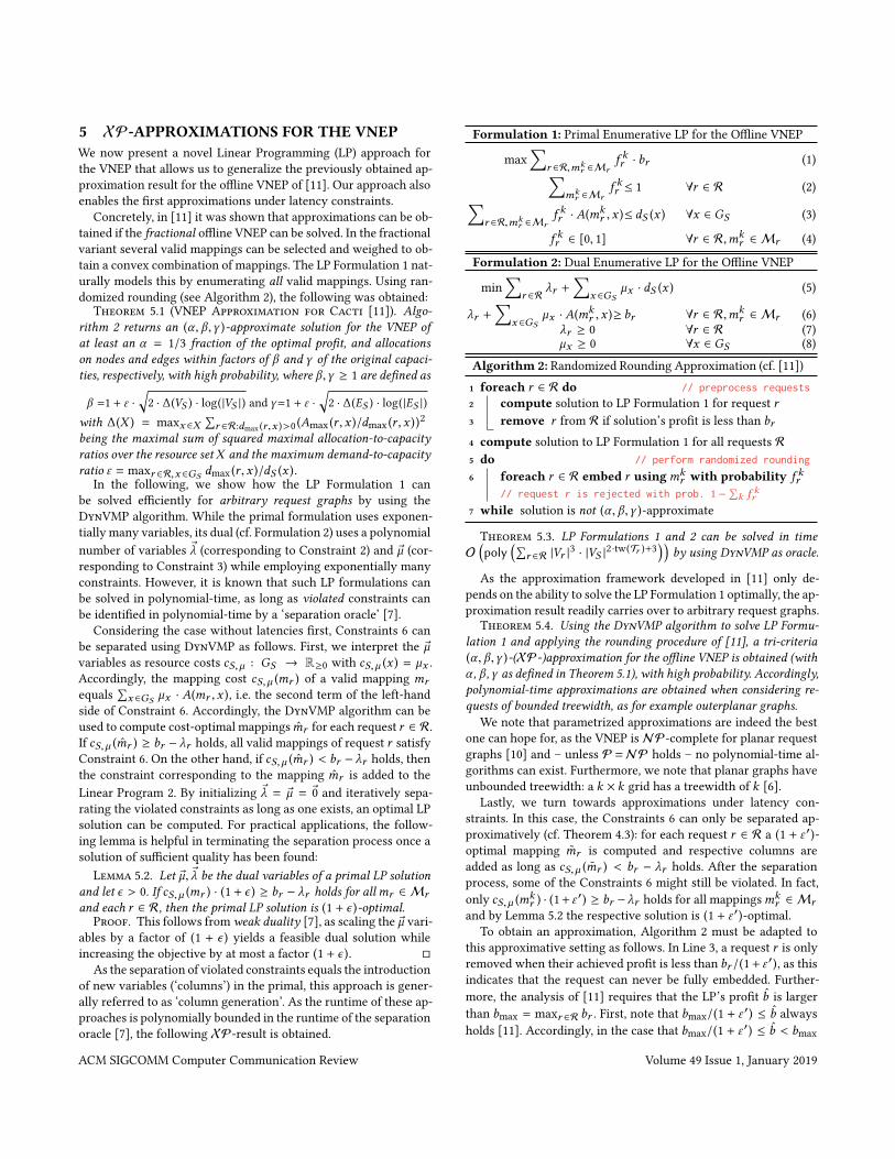
Formulation 1: Primal Enumerative LP for the Offline VNEP

max(

r ∈R,mkr ∈Mr

f kr · br (1)(

mkr ∈Mr

f kr ≤ 1 ∀r ∈ R (2)(

r ∈R,mkr ∈Mr

f kr · A(mkr ,x )≤ dS (x ) ∀x ∈ GS (3)

f kr ∈ [0, 1] ∀r ∈ R,mkr ∈Mr (4)

Formulation 2: Dual Enumerative LP for the Offline VNEP

min(

r ∈R λr +(

x ∈GSµx · dS (x ) (5)

λr +(

x ∈GSµx · A(mk

r ,x )≥ br ∀r ∈ R,mkr ∈Mr (6)

λr ≥ 0 ∀r ∈ R (7)µx ≥ 0 ∀x ∈ GS (8)

Algorithm 2: Randomized Rounding Approximation (cf. [11])1 foreach r ∈ R do // preprocess requests

2 compute solution to LP Formulation 1 for request r3 remove r from R if solution’s profit is less than br4 compute solution to LP Formulation 1 for all requests R5 do // perform randomized rounding

6 foreach r ∈ R embed r usingmkr with probability f kr

// request r is rejected with prob. 1 −!k f kr

7 while solution is not (α , β ,γ )-approximate

Theorem 5.3. LP Formulations 1 and 2 can be solved in timeO

%poly

%!r ∈R |Vr |3 · |VS |2·tw(Tr )+3

&&by using DynVMP as oracle.

As the approximation framework developed in [11] only de-pends on the ability to solve the LP Formulation 1 optimally, the ap-proximation result readily carries over to arbitrary request graphs.

Theorem 5.4. Using the DynVMP algorithm to solve LP Formu-lation 1 and applying the rounding procedure of [11], a tri-criteria(α , β ,γ )-(XP-)approximation for the offline VNEP is obtained (withα , β ,γ as defined in Theorem 5.1), with high probability. Accordingly,polynomial-time approximations are obtained when considering re-quests of bounded treewidth, as for example outerplanar graphs.

We note that parametrized approximations are indeed the bestone can hope for, as the VNEP isNP-complete for planar requestgraphs [10] and – unless P =NP holds – no polynomial-time al-gorithms can exist. Furthermore, we note that planar graphs haveunbounded treewidth: a k × k grid has a treewidth of k [6].

Lastly, we turn towards approximations under latency con-straints. In this case, the Constraints 6 can only be separated ap-proximatively (cf. Theorem 4.3): for each request r ∈ R a (1 + ε ′)-optimal mapping mr is computed and respective columns areadded as long as cS,µ (mr ) < br − λr holds. After the separationprocess, some of the Constraints 6 might still be violated. In fact,only cS,µ (mk

r ) · (1+ ε ′) ≥ br −λr holds for all mappingsmkr ∈Mr

and by Lemma 5.2 the respective solution is (1 + ε ′)-optimal.To obtain an approximation, Algorithm 2 must be adapted to

this approximative setting as follows. In Line 3, a request r is onlyremoved when their achieved profit is less than br /(1+ ε ′), as thisindicates that the request can never be fully embedded. Further-more, the analysis of [11] requires that the LP’s profit b is largerthan bmax = maxr ∈R br . First, note that bmax/(1 + ε ′) ≤ b alwaysholds [11]. Accordingly, in the case that bmax/(1 + ε ′) ≤ b < bmax


holds, an additional profit of bmax−b must be ensured. This can beachieved by adding a fractional embedding of the request rmax ∈ Rhaving the largest profit. In particular, given the initial LP compu-tation for rmax of Line 2, the returned solution can be scaled to fullyembed rmax while exceeding capacities by at most a factor (1+ ε ′).Adding a (bmax − b)/bmax ≤ ε ′/(1+ ε ′) fraction of this embeddingto LP solution of Line 4, the condition b ≥ bmax holds while the LPsolution exceeds capacities by at most a factor (1 + ε ′). Roundingthis solution as before, the following approximation is obtained:

Theorem 5.5. For the offline VNEP with latency constraints,a tri-criteria (α/(1 + ε ′), β + ε ′,γ + ε ′)-(XP-)approximation is ob-tained for any ε ′ > 0 and α , β , γ as defined in Theorem 5.1,with high probability. The runtime of the algorithm lies inO

%poly

%!r ∈R |Vr |2 ·

%|Vr | · |VS |2·tw(Tr )+2 + timeLCSP (ε ′)

&&&.

6 RANDOMIZED ROUNDING HEURISTICSThe approximations come at the cost of violating resource capac-ities. However, randomized rounding can be easily adapted to ob-tain XP-heuristics not violating resource capacities. In [11] a firstheuristic was proposed, which works as Algorithm 2 but discardsselected mappings whose addition would exceed capacities.

As an improvement over this heuristic and facilitated by the col-umn generation approach, we propose a novel rounding heuris-tic that a priori removes mappings whose addition would lead toresource violations and recomputes the LP before applying therounding (see Algorithm 3). Therefore, the addition of any roundedmapping is feasible while also better guiding the rounding processby providing currently optimal rounding probabilities. Specifically,in Lines 4 and 5 first all infeasible mappings are ‘removed’ by set-ting the respective LP variables to 0. To reflect made rounding de-cisions in the LP, either the respective mapping variable is set to 1(Line 9), or all mappings of a rejected request are disabled (Line 11).

Besides this novel rounding heuristic, we also consider differentorders to round request mappings in: randomized (R) as proposedin [11], and either sorting the requests in descending fashion bytheir static (S) profits or their actual achieved profit (A) in the LP.Algorithm 3: Heuristical Rounding with LP Recomputation1 compute solution to LP 1 (using column generation)2 set sol← ∅ and R ′ ← R3 foreach r ∈ R do4 foreach r ′ ∈ R ′ and eachmk

r ′ ∈Mr ′ do5 if sol ∪ {mk

r } is infeasible then set f kr ′ = 06 resolve Linear Program (without column generation)7 choose mr ←mk

r with probability f kr8 if mr ! ∅ then9 set sol← sol∪ {mr } and f kr = 1 // accept request r

10 else11 set f kr = 0 for allmk

r ∈Mr // reject request r

12 R ′ ← R \ {r }13 return sol

7 EVALUATIONIn this section we present two types of evaluation to validate ourapproach. Firstly, we present a study of the treewidth of random

5 15 25 35 451uPEer of 1odes

10 %20 %30 %40 %50 %60 %70 %80 %90 %

Edge

3ro

EaEi

lity

Average 7reewidth

1

2 3 4 6 10

20

40

0 5 10 15 20 25 30 35 40 457reewidth

10−1

100

101

5unt

ime

[s]

DecRmpRsitiRn 5untimepercentiles

99% - 100%75% - 99%25% - 75%1% - 25%0% - 1%

mediDn

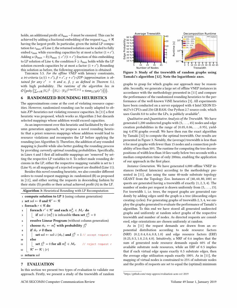
Figure 3: Study of the treewidth of random graphs usingTamaki’s algorithm [12]. Note the logarithmic axes.

graphs to grasp for which graphs our approach may be reason-able. Secondly, we generate a large set of offline VNEP instances inaccordance with the methodology presented in [11] and comparethe performance of the randomized rounding heuristics to the per-formance of the well-known ViNE heuristics [3]. All experimentshave been conducted on a server equipped with 4 Intel XEON E5-4627v3 CPUs and 256 GB RAM. Our Python 2.7 source code, whichuses Gurobi 8.0 to solve the LPs, is publicly available1.

Qualitative and Quantitative Analysis of the Treewidth. We havegenerated 1,200 undirected graphs with {5, . . . , 45} nodes and edgecreation probabilities in the range of {0.05, 0.06, . . . , 0.95}, yield-ing 4.47M graphs overall. We have then run the exact algorithmby Tamaki [12] to compute the optimal treewidth. Our results arepresented in Figure 3. Notably, the (average) treewidth is less than6 for most graphs with fewer than 15 nodes and a connection prob-ability of less than 50%. The runtime for computing the tree decom-positions of width less than 10 lies vastly below two seconds with amedian computation time of only 200ms, enabling the applicationof our approach in the first place.

Instance Generation. We have generated 6,000 offline VNEP in-stances (without latencies) according to the methodology pre-sented in [11], also using the same 40-node substrate topologyGÉANT from the Topology Zoo. Instances of {40, 60, 80, 100} re-quests are generated having a treewidth of exactly {1, 2, 3, 4}. Thenumber of nodes per request is drawn uniformly from {5, . . . , 15}.For treewidth 1, i.e. trees, the request graphs are generated ran-domly by adding edges until the graph is a tree (discarding edgescreating cycles). For generating graphs of treewidth 2, 3, 4, we em-ploy the graphs generated to evaluate the performance of Tamaki’salgorithm. To this end we have stored all generated undirectedgraphs and uniformly at random select graphs of the respectivetreewidth and number of nodes. As directed requests are consid-ered, edge orientations are chosen uniformly at random.

As in [11] the request demands are drawn from an ex-ponential distribution according to node resource factors(NRF) {0.2, 0.4, 0.6, 0.8, 1.0} and edge resource factors (ERF){0.25, 0.5, 1.0, 2.0, 4.0}. Intuitively, a NRF of 0.6 implies that thesum of generated node resource demands equals 60% of theavailable substrate node resources, while an ERF of 0.5 impliesthat if each virtual edge spans exactly 0.5 substrate edges, thenthe average edge utilization equals exactly 100%. As in [11], themapping of virtual nodes is constrained to 25% of substrate nodesand the profits of requests are set to equal the (optimal) minimum

1https://github.com/vnep-approx/evaluation-acm-ccr-2019


https://github.com/vnep-approx/evaluation-acm-ccr-2019

0

20

40

60

80

100

PURf

LW / /

P 8%

[%]

C / C /DHW. RDnd.

WL1((VL1()

R 6 A R 6 A1R RHcRPS. RHcRPS.

RR HHuULVWLcV

EHVWPHDn

PHUfRUPDncH Rf AlgRULWhP VDULDnWV

40 60 80 1001uPEeU RI 5equesWs

0.25

0.5

1.0

2.0

4.0

(dge

5es

RuUF

e )a

FWRU

5el. IPpURv.: (55EesW - :L1(EesW)//P8% [%]

-24-18-12-6 0 6 12 18 24

0255075

100 #req.:40 & 60#req.:40 & 60#req.:40 & 60#req.:40 & 60#req.:40 & 60

40 70 100 130 160 190prRfiW(55EesW) / prRfiW(:i1(EesW) [%]

0255075

100 #req.:80 & 100#req.:80 & 100#req.:80 & 100#req.:80 & 100#req.:80 & 100

(5)0.250.51.02.04.0

(5)0.250.51.02.04.0

(&D

) [%

]

3rRfiW &RPpDrisRn: 55EesW / :i1(EesW

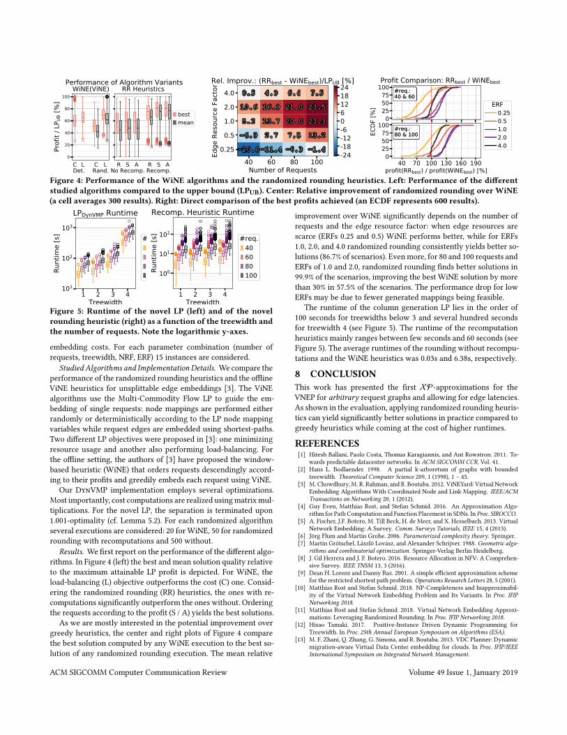
Figure 4: Performance of the WiNE algorithms and the randomized rounding heuristics. Left: Performance of the differentstudied algorithms compared to the upper bound (LPUB). Center: Relative improvement of randomized rounding over WiNE(a cell averages 300 results). Right: Direct comparison of the best profits achieved (an ECDF represents 600 results).

1 2 3 4TreewLdth

101

102

103

Runt

LPe

[V]

L3DynV03 RuntLPe

#reT.406080100

#reT.406080100

1 2 3 4TrHHwidth

100

101

102

Runt

imH

[s]

RHcRmp. HHuristic RuntimH

#rHT.406080100

#rHT.406080100

Figure 5: Runtime of the novel LP (left) and of the novelrounding heuristic (right) as a function of the treewidth andthe number of requests. Note the logarithmic y-axes.

embedding costs. For each parameter combination (number ofrequests, treewidth, NRF, ERF) 15 instances are considered.

Studied Algorithms and Implementation Details. We compare theperformance of the randomized rounding heuristics and the offlineViNE heuristics for unsplittable edge embeddings [3]. The ViNEalgorithms use the Multi-Commodity Flow LP to guide the em-bedding of single requests: node mappings are performed eitherrandomly or deterministically according to the LP node mappingvariables while request edges are embedded using shortest-paths.Two different LP objectives were proposed in [3]: one minimizingresource usage and another also performing load-balancing. Forthe offline setting, the authors of [3] have proposed the window-based heuristic (WiNE) that orders requests descendingly accord-ing to their profits and greedily embeds each request using ViNE.

Our DynVMP implementation employs several optimizations.Most importantly, cost computations are realized usingmatrixmul-tiplications. For the novel LP, the separation is terminated upon1.001-optimality (cf. Lemma 5.2). For each randomized algorithmseveral executions are considered: 20 for WiNE, 50 for randomizedrounding with recomputations and 500 without.

Results. We first report on the performance of the different algo-rithms. In Figure 4 (left) the best and mean solution quality relativeto the maximum attainable LP profit is depicted. For WiNE, theload-balancing (L) objective outperforms the cost (C) one. Consid-ering the randomized rounding (RR) heuristics, the ones with re-computations significantly outperform the ones without. Orderingthe requests according to the profit (S / A) yields the best solutions.

As we are mostly interested in the potential improvement overgreedy heuristics, the center and right plots of Figure 4 comparethe best solution computed by any WiNE execution to the best so-lution of any randomized rounding execution. The mean relative

improvement over WiNE significantly depends on the number ofrequests and the edge resource factor: when edge resources arescarce (ERFs 0.25 and 0.5) WiNE performs better, while for ERFs1.0, 2.0, and 4.0 randomized rounding consistently yields better so-lutions (86.7% of scenarios). Evenmore, for 80 and 100 requests andERFs of 1.0 and 2.0, randomized rounding finds better solutions in99.9% of the scenarios, improving the best WiNE solution by morethan 30% in 57.5% of the scenarios. The performance drop for lowERFs may be due to fewer generated mappings being feasible.

The runtime of the column generation LP lies in the order of100 seconds for treewidths below 3 and several hundred secondsfor treewidth 4 (see Figure 5). The runtime of the recomputationheuristics mainly ranges between few seconds and 60 seconds (seeFigure 5). The average runtimes of the rounding without recompu-tations and the WiNE heuristics was 0.03s and 6.38s, respectively.

8 CONCLUSIONThis work has presented the first XP-approximations for theVNEP for arbitrary request graphs and allowing for edge latencies.As shown in the evaluation, applying randomized rounding heuris-tics can yield significantly better solutions in practice compared togreedy heuristics while coming at the cost of higher runtimes.

REFERENCES[1] Hitesh Ballani, Paolo Costa, Thomas Karagiannis, and Ant Rowstron. 2011. To-

wards predictable datacenter networks. In ACM SIGCOMM CCR, Vol. 41.[2] Hans L. Bodlaender. 1998. A partial k-arboretum of graphs with bounded

treewidth. Theoretical Computer Science 209, 1 (1998), 1 – 45.[3] M. Chowdhury,M. R. Rahman, and R. Boutaba. 2012. ViNEYard: Virtual Network

Embedding Algorithms With Coordinated Node and Link Mapping. IEEE/ACMTransactions on Networking 20, 1 (2012).

[4] Guy Even, Matthias Rost, and Stefan Schmid. 2016. An Approximation Algo-rithm for Path Computation and Function Placement in SDNs. In Proc. SIROCCO.

[5] A. Fischer, J.F. Botero, M. Till Beck, H. de Meer, and X. Hesselbach. 2013. VirtualNetwork Embedding: A Survey. Comm. Surveys Tutorials, IEEE 15, 4 (2013).

[6] Jörg Flum and Martin Grohe. 2006. Parameterized complexity theory. Springer.[7] Martin Grötschel, László Lovász, and Alexander Schrijver. 1988. Geometric algo-

rithms and combinatorial optimization. Springer-Verlag Berlin Heidelberg.[8] J. Gil Herrera and J. F. Botero. 2016. Resource Allocation in NFV: A Comprehen-

sive Survey. IEEE TNSM 13, 3 (2016).[9] Dean H. Lorenz and Danny Raz. 2001. A simple efficient approximation scheme

for the restricted shortest path problem. Operations Research Letters 28, 5 (2001).[10] Matthias Rost and Stefan Schmid. 2018. NP-Completeness and Inapproximabil-

ity of the Virtual Network Embedding Problem and Its Variants. In Proc. IFIPNetworking 2018.

[11] Matthias Rost and Stefan Schmid. 2018. Virtual Network Embedding Approxi-mations: Leveraging Randomized Rounding. In Proc. IFIP Networking 2018.

[12] Hisao Tamaki. 2017. Positive-Instance Driven Dynamic Programming forTreewidth. In Proc. 25th Annual European Symposium on Algorithms (ESA).

[13] M. F. Zhani, Q. Zhang, G. Simona, and R. Boutaba. 2013. VDC Planner: Dynamicmigration-aware Virtual Data Center embedding for clouds. In Proc. IFIP/IEEEInternational Symposium on Integrated Network Management.


Parametrized Complexity of Virtual Network Embeddings ... · Parametrized Complexity of Virtual...

Documents

Transcript of Parametrized Complexity of Virtual Network Embeddings ... · Parametrized Complexity of Virtual...