PARAMETRIC OPTIMIZATION OF FUSED DEPOSITION

MODELING USING RESPONSE SURFACE METHODOLOGY

A THESIS SUBMITTED IN PARTIAL FULFILLMENT

FOR THE REQUIREMENT FOR THE DEGREE OF

Master of Technology

in

Production Engineering

by

VEDANSH CHATURVEDI

Department of Mechanical Engineering

National Institute of Technology

Rourkela – 8

2009

PARAMETRIC OPTIMIZATION OF FUSED DEPOSITION

MODELING USING RESPONSE SURFACE METHODOLOGY

A THESIS SUBMITTED IN PARTIAL FULFILLMENT

FOR THE REQUIREMENT FOR THE DEGREE OF

Master of Technology

in

Production Engineering

by

VEDANSH CHATURVEDI

Under the guidance of

Dr. S. S. MAHAPATRA

Professor, Department of Mechanical Engineering

Department of Mechanical Engineering

National Institute of Technology

Rourkela – 8

2009

National Institute of Technology

Rourkela

CERTIFICATE

This is to certify that the thesis entitled, “PARAMETRIC OPTIMIZATION OF

FUSED MODELING USING RESPONSE SURFACE METHODOLOGY”

submitted by Vedansh Chaturvedi in partial fulfillment of the requirements for the

award of Master of Technology Degree in Mechanical Engineering with

specialization in Production Engineering at the National Institute of Technology,

Rourkela (deemed University) is an authentic work carried out by him under my

supervision and guidance.

To the best of my knowledge, the matter embodied in the thesis has not submitted

to any other University/Institute for the award of any degree or diploma.

Dr. S. S. Mahapatra

Date: Dept. of Mechanical Engineering

National Institute of Technology

Rourkela – 769008

ACKNOWLEDGEMENT

I would like to express my deep sense of respect and gratitude toward my supervisor Dr. S. S.

Mahapatra, who not only guided the academic project work but also stood as a teacher and

philosopher in realizing the imagination in pragmatic way, I want to thank him for introducing

me for the field of Optimization and giving the opportunity to work under him. His presence and

optimism have provided an invaluable influence on my career and outlook for the future. I

consider it my good fortune to have got an opportunity to work with such a wonderful person.

I express my gratitude to Dr. R. K. Sahoo, Professor and Head, Department of Mechanical

Engineering, faculty member and staff of Department of Mechanical Engineering for extending

all possible help in carrying out the dissertation work directly or indirectly. They have been great

source of inspiration to me and I thank them from bottom of my heart. I like to express my

gratitude to Dr. Saurav Datta, Lecturer, Department of Mechanical Engineering , for his

valuable advice in carrying out Literature review.

I am especially indebted to my parents for their love, sacrifices and support. They are my

teachers after I came to this world and have set great example for me about how to live, study

and work.

VEDANSH CHATURVEDI

i

CONTENTS

TITLE PAGE NO.

Abstract iv

List of Figures v

List of Tables vii

Nomenclature viii

1. An introduction of rapid prototyping process 1

1.1 Overview of rapid prototyping process 1

1.2 The basic process 2

1.3 Rapid prototyping technique 4

1.3.1 Stereolithography 4

1.3.2 Selective layer sintering 6

1.3.3 Laminated object manufacturing 8

1.3.4 Fused deposition modeling 11

1.4 Objective of Research Work 12

2. Literature review 15

3. Fused deposition modeling and ABS material 20

3.1 Fused deposition modeling 20

3.2 ABS material 23

3.3 Properties of ABS plastic 24

4. Response surface methodology 27

4.1 Response surface methodology and robust design 30

ii

4.2 The sequential nature of the response surface methodology 31

4.3 Building empirical models 32

4.3.1 Linear regression model 32

4.3.2 Estimation of the parameter in linear regression model 33

4.3.3 Model adequacy checking 34

4.3.4 Properties of the least square estimation regression model 34

4.3.5 Residual analysis 36

4.4 Variable selection and model building in regression 37

4.4.1 Procedure for variable selection 38

4.4.2 All possible regression 38

4.4.3 Stepwise regression analysis 39

5. Specimen preparation, Experiment and analysis 41

5.1 Specimen preparation 41

5.2 Testing of specimen 43

5.3 Analysis of experiments 47

5.3.1 Analysis of experiment for tensile test 47

5.3.2 RSA for tensile test 49

5.3.3 Analysis of experiment for flexural test 53

5.3.4 RSA for flexural test 54

5.3.5 Analysis of experiment for impact test 58

5.3.6 RSA for impact test 59

5.4 Optimization of process parameter 62

iii

6. Grey- based taguchi method 64

6.1 Introduction of grey – based taguchi method 64

6.2 Grey relational analysis method 65

6.3 Response optimization of GRG and optimal parameter setting 75

7. Result, Conclusion and future scope 77

7.1 Result, Discussion 77

7.2 Conclusion 80

7.3 Future scope 80

Bibliography 81

iv

ABSTRACT

Fused deposition modeling (FDM) is a process for developing rapid prototype (RP) objects by

depositing fused layers of material according to numerically defined cross sectional geometry.

The quality of FDM produced parts is significantly affected by various parameters used in the

process. This dissertation work aims to study the effect of five process parameters such as layer

thickness, sample orientation, raster angle, raster width, and air gap on mechanical property of

FDM processed parts. In order to reduce experimental runs, response surface methodology

(RSM) based on central composite design is adopted. Specimens are prepared for tensile,

flexural, and impact test as per ASTM standards. Empirical relations among responses and

process parameters are determined and their validity is proved using analysis of variance

(ANOVA) and the normal probability plot of residuals. Response surface plots are analyzed to

establish main factor effects and their interaction on responses. Optimal factor settings for

maximization of each response have been determined. Major reason for weak strength of FDM

processed parts may be attributed to distortion within the layer or between the layers while

building the parts due to temperature gradient. Since RP parts are subjected to different loading

conditions, practical implication suggests that more than one response must be optimized

simultaneously. To this end, mechanical properties like tensile strength, bending strength, and

impact strength of the produced component are considered as multiple responses and

simultaneous optimization has been carried out with the help of response optimizer. Grey

relation has been employed to convert multiple responses into a single response for optimization

purpose. It is interesting to note that factor level settings for simultaneous optimization of all

responses significantly differ from optimization with single response.

v

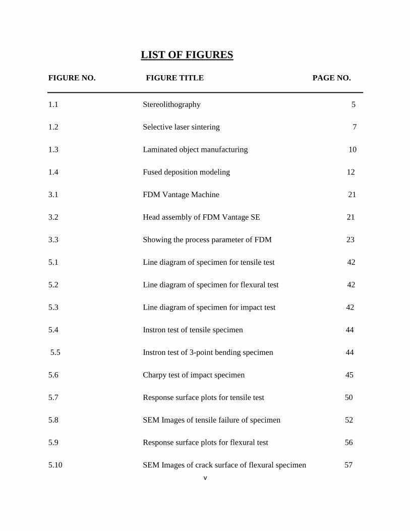
LIST OF FIGURES

FIGURE NO. FIGURE TITLE PAGE NO.

1.1 Stereolithography 5

1.2 Selective laser sintering 7

1.3 Laminated object manufacturing 10

1.4 Fused deposition modeling 12

3.1 FDM Vantage Machine 21

3.2 Head assembly of FDM Vantage SE 21

3.3 Showing the process parameter of FDM 23

5.1 Line diagram of specimen for tensile test 42

5.2 Line diagram of specimen for flexural test 42

5.3 Line diagram of specimen for impact test 42

5.4 Instron test of tensile specimen 44

5.5 Instron test of 3-point bending specimen 44

5.6 Charpy test of impact specimen 45

5.7 Response surface plots for tensile test 50

5.8 SEM Images of tensile failure of specimen 52

5.9 Response surface plots for flexural test 56

5.10 SEM Images of crack surface of flexural specimen 57

vi

5.11 Response surface plots for impact test 61

5.12 SEM Images of broke impact test specimen 61

6.1 Sensitivity analysis for different distinguishing coefficients 72

6.2 Grey relational grade variation with number of experiments 72

vii

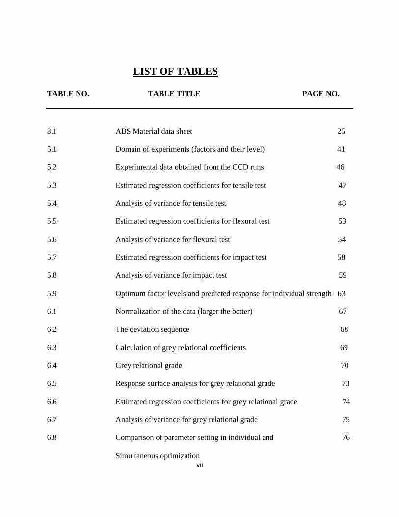
LIST OF TABLES

TABLE NO. TABLE TITLE PAGE NO.

3.1 ABS Material data sheet 25

5.1 Domain of experiments (factors and their level) 41

5.2 Experimental data obtained from the CCD runs 46

5.3 Estimated regression coefficients for tensile test 47

5.4 Analysis of variance for tensile test 48

5.5 Estimated regression coefficients for flexural test 53

5.6 Analysis of variance for flexural test 54

5.7 Estimated regression coefficients for impact test 58

5.8 Analysis of variance for impact test 59

5.9 Optimum factor levels and predicted response for individual strength 63

6.1 Normalization of the data (larger the better) 67

6.2 The deviation sequence 68

6.3 Calculation of grey relational coefficients 69

6.4 Grey relational grade 70

6.5 Response surface analysis for grey relational grade 73

6.6 Estimated regression coefficients for grey relational grade 74

6.7 Analysis of variance for grey relational grade 75

6.8 Comparison of parameter setting in individual and 76

Simultaneous optimization

viii

NOMENCLATURE

RP Rapid prototyping

STL Stereolithography

FDM Fused deposition modeling

ABS Acrylonitrile butadiene styrene

RSM Response surface methodology

CCD Central composite design

ANOVA Analysis of variance

SS Sum of square

MS Mean sum of square

DF Degree of freedom

SEM Scanning electron microscope

GRA Grey relational analysis

GRG Grey relational grade

CHAPTER 1

______________________________________________________________________________

AN INTRODUCTION TO

RAPID PROTOTYPING

1

1. Introduction

1.1 Overview of Rapid Prototyping:

The term rapid prototyping (RP) refers to a class of technologies that can automatically construct

physical models from Computer-Aided Design (CAD) data. These "three dimensional printers"

allow designers to quickly create tangible prototypes of their designs, rather than just two-

dimensional pictures. Such models have numerous uses. They make excellent visual aids for

communicating ideas with co-workers or customers. In addition, prototypes can be used for

design testing. For example, an aerospace engineer might mount a model airfoil in a wind tunnel

to measure lift and drag forces. Designers have always utilized prototypes; RP allows them to be

made faster and less expensively.

In addition to prototypes, RP techniques can also be used to make tooling (referred to as rapid

tooling) and even production-quality parts (rapid manufacturing). For small production runs and

complicated objects, rapid prototyping is often the best manufacturing process available. Of

course, "rapid" is a relative term. Most prototypes require from three to seventy-two hours to

build, depending on the size and complexity of the object. This may seem slow, but it is much

faster than the weeks or months required to make a prototype by traditional means such as

machining. These dramatic time savings allow manufacturers to bring products to market faster

and more cheaply. In 1994, Pratt & Whitney achieved "an order of magnitude [cost] reduction

[and] . . . time savings of 70 to 90 percent" by incorporating rapid prototyping into their

investment casting process.

At least six different rapid prototyping techniques are commercially available, each with unique

strengths. Because RP technologies are being increasingly used in non-prototyping applications,

2

the techniques are often collectively referred to as solid free-form fabrication; computer

automated manufacturing, or layered manufacturing. The latter term is particularly descriptive of

the manufacturing process used by all commercial techniques. A software package "slices" the

CAD model into a number of thin (~0.1 mm) layers, which are then built up one atop another.

Rapid prototyping is an "additive" process, combining layers of paper, wax, or plastic to create a

solid object. In contrast, most machining processes (milling, drilling, grinding, etc.) are

"subtractive" processes that remove material from a solid block. RP’s additive nature allows it to

create objects with complicated internal features that cannot be manufactured by other means.

Of course, rapid prototyping is not perfect. Part volume is generally limited to 0.125 cubic

meters or less, depending on the RP machine. Metal prototypes are difficult to make, though this

should change in the near future. For metal parts, large production runs, or simple objects,

conventional manufacturing techniques are usually more economical. These limitations aside,

rapid prototyping is a remarkable technology that is revolutionizing the manufacturing process.

1.2 The Basic Process

Although several rapid prototyping techniques exist, all employ the same basic five-step process.

The steps are:

1. Create a CAD model of the design

2. Convert the CAD model to STL format

3. Slice the STL file into thin cross-sectional layers

4. Construct the model one layer atop another

5. Clean and finish the model

3

CAD Model Creation: First, the object to be built is modeled using a Computer-Aided Design

(CAD) software package. Solid modelers, such as Pro/ENGINEER, tend to represent 3-D objects

more accurately than wire-frame modelers such as AutoCAD, and will therefore yield better

results. The designer can use a pre-existing CAD file or may wish to create one expressly for

prototyping purposes. This process is identical for all of the RP build techniques.

Conversion to STL Format: The various CAD packages use a number of different algorithms

to represent solid objects. To establish consistency, the STL (stereolithography), the first RP

technique) format has been adopted as the standard of the rapid prototyping industry. The second

step, therefore, is to convert the CAD file into STL format. This format represents a three-

dimensional surface as an assembly of planar triangles, "like the facets of a cut jewel." The file

contains the coordinates of the vertices and the direction of the outward normal of each triangle.

Because STL files use planar elements, they cannot represent curved surfaces exactly. Increasing

the number of triangles improves the approximation, but at the cost of bigger file size. Large,

complicated files require more time to pre-process and build, so the designer must balance

accuracy with manageability to produce a useful STL file. Since the .stl format is universal, this

process is identical for all of the RP build techniques.

Slice the STL File: In the third step, a pre-processing program prepares the STL file to be built.

Several programs are available, and most allow the user to adjust the size, location and

orientation of the model. Build orientation is important for several reasons. First, properties of

rapid prototypes vary from one coordinate direction to another. For example, prototypes are

usually weaker and less accurate in the z (vertical) direction than in the x-y plane. In addition,

part orientation partially determines the amount of time required to build the model. Placing the

shortest dimension in the z direction reduces the number of layers, thereby shortening build time.

4

The pre-processing software slices the STL model into a number of layers from 0.01 mm to 0.7

mm thick, depending on the build technique. The program may also generate an auxiliary

structure to support the model during the build. Supports are useful for delicate features such as

overhangs, internal cavities, and thin-walled sections. Each PR machine manufacturer supplies

their own proprietary pre-processing software.

Layer by Layer Construction: The fourth step is the actual construction of the part. Using one

of several techniques (described in the next section) RP machines build one layer at a time from

polymers, paper, or powdered metal. Most machines are fairly autonomous, needing little human

intervention.

Clean and Finish: The final step is post-processing. This involves removing the prototype from

the machine and detaching any supports. Some photosensitive materials need to be fully cured

before use. Prototypes may also require minor cleaning and surface treatment. Sanding, sealing,

and/or painting the model will improve its appearance and durability.

1.3 Rapid Prototyping Techniques

Most commercially available rapid prototyping machines use one of six techniques. At present,

trade restrictions severely limit the import/export of rapid prototyping machines, so this guide

only covers systems available in the U.S.

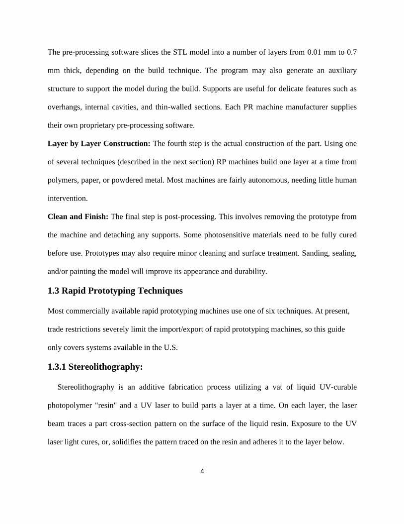
1.3.1 Stereolithography:

Stereolithography is an additive fabrication process utilizing a vat of liquid UV-curable

photopolymer "resin" and a UV laser to build parts a layer at a time. On each layer, the laser

beam traces a part cross-section pattern on the surface of the liquid resin. Exposure to the UV

laser light cures, or, solidifies the pattern traced on the resin and adheres it to the layer below.

5

After a pattern has been traced, the SLA's elevator platform descends by a single layer thickness,

typically 0.05 mm to 0.15 mm (0.002" to 0.006"). Then, a resin-filled blade sweeps across the

part cross section, re-coating it with fresh material. On this new liquid surface the subsequent

layer pattern is traced, adhering to the previous layer. A complete 3-D part is formed by this

process. After building, parts are cleaned of excess resin by immersion in a chemical bath and

then cured in a UV oven.

Stereolithography requires the use of support structures to attach the part to the elevator platform

and to prevent certain geometry from not only deflecting due to gravity, but to also accurately

hold the 2-D cross sections in place such that they resist lateral pressure from the re-coater blade.

Supports are generated automatically during the preparation of 3-D CAD models for use on the

stereolithography machine, although they may be manipulated manually. Supports must be

removed from the finished product manually; this is not true for all rapid prototyping

technologies.

Figure 1.1 Stereolithography

Application Range

Parts used for functional tests.

6

Manufacturing of medical models.

Form –fit functions for assembly tests.

Advantages

Possibility of manufacturing parts which are impossible to be produced

conventionally in a single process.

Can be fully atomized and no supervision is required.

High Resolution.

Disadvantages

Necessity to have a support structure.

Require labor for post processing and cleaning.

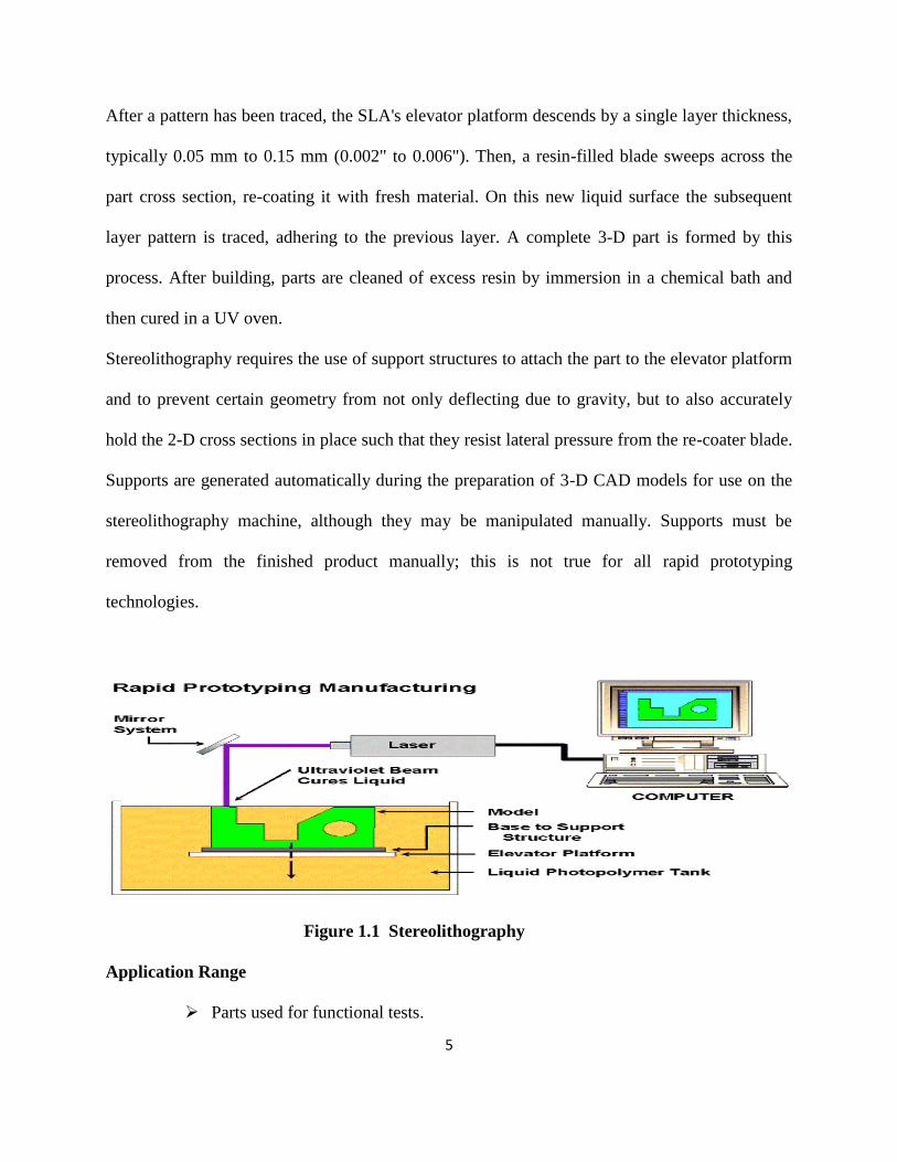
1.3.2 Selective Laser Sintering:

Selective laser sintering is an additive rapid manufacturing technique that uses a high power

laser (for example, a carbon dioxide laser) to fuse small particles of plastic, metal, ceramic, or

glass powders into a mass representing a desired 3-dimensional object. The laser selectively

fuses powdered material by scanning cross-sections generated from a 3-D digital description of

the part (for example from a CAD file or scan data) on the surface of a powder bed. After each

cross-section is scanned, the powder bed is lowered by one layer thickness, a new layer of

material is applied on top, and the process is repeated until the part is completed.Compared to

other rapid manufacturing methods, SLS can produce parts from a relatively wide range of

commercially available powder materials, including polymers (nylon, also glass-filled or with

other fillers, and polystyrene), metals (steel, titanium, alloy mixtures, and composites) and green

sand. The physical process can be full melting, partial melting, or liquid-phase sintering. And,

7

depending on the material, up to 100% density can be achieved with material properties

comparable to those from conventional manufacturing methods. In many cases large numbers of

parts can be packed within the powder bed, allowing very high productivity.SLS is performed by

machines called SLS systems; the most widely known model of which is the Sinterstation SLS

system. SLS technology is in wide use around the world due to its ability to easily make very

complex geometries directly from digital CAD data. While it began as a way to build prototype

parts early in the design cycle, it is increasingly being used in limited-run manufacturing to

produce end-use parts. One less expected and rapidly growing application of SLS is its use in art.

SLS was developed and patented by Dr. Carl Deckard at the University of Texas at Austin in the

mid-1980s, under sponsorship of DARPA. A similar process was patented without being

commercialized by R.F. Housholder in 1979.Unlike some other Rapid Prototyping processes,

such as Stereolithography (SLA) and Fused Deposition Modeling (FDM), SLS does not require

support structures due to the fact that the part being constructed is surrounded by unsintered

powder at all times.

Figure 1.2 Selective laser sintering

8

Application Range

Visual Representation models.

Functional and tough prototypes.

cast metal parts.

Advantages

Flexibility of materials used.

No need to create a structure to support the part.

Parts do not require any post curing except when ceramic is used.

Disadvantages

During solidification, additional powder may be hardened at the border line.

The roughness is most visible when parts contain sloping (stepped) surfaces.

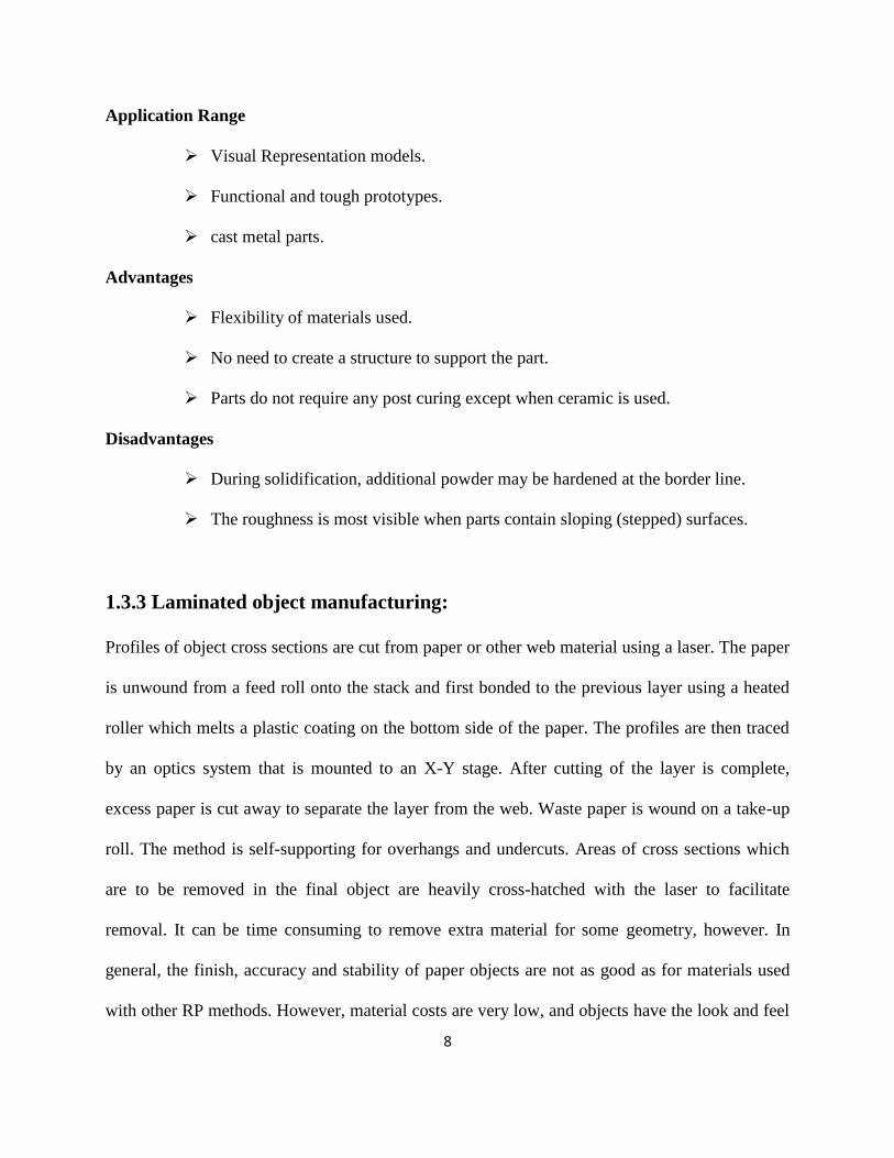
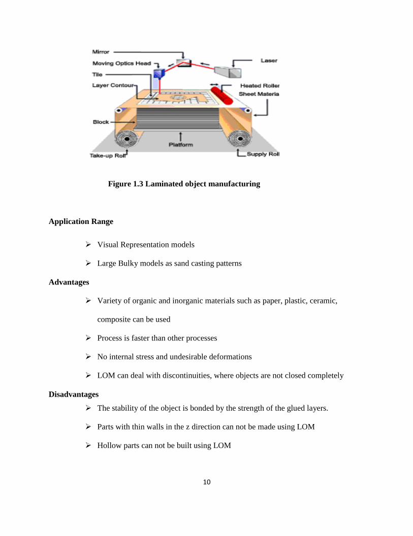
1.3.3 Laminated object manufacturing:

Profiles of object cross sections are cut from paper or other web material using a laser. The paper

is unwound from a feed roll onto the stack and first bonded to the previous layer using a heated

roller which melts a plastic coating on the bottom side of the paper. The profiles are then traced

by an optics system that is mounted to an X-Y stage. After cutting of the layer is complete,

excess paper is cut away to separate the layer from the web. Waste paper is wound on a take-up

roll. The method is self-supporting for overhangs and undercuts. Areas of cross sections which

are to be removed in the final object are heavily cross-hatched with the laser to facilitate

removal. It can be time consuming to remove extra material for some geometry, however. In

general, the finish, accuracy and stability of paper objects are not as good as for materials used

with other RP methods. However, material costs are very low, and objects have the look and feel

9

of wood and can be worked and finished in the same manner. This has fostered applications such

as patterns for sand castings. While there are limitations on materials, work has been done with

plastics, composites, ceramics and metals. Some of these materials are available on a limited

commercial basis. Variations on this method have been developed by many companies and

research groups. For example, Kira's Paper Lamination Technology (PLT) uses a knife to cut

each layer instead of a laser and applies adhesive to bond layers using the xerographic process.

Solido Ltd. of Israel (formerly Solidimension) also uses a knife, but instead bonds layers of

plastic film with a solvent. There are also variations which seek to increase speed and/or material

versatility by cutting the edges of thick layers diagonally to avoid stair stepping. The principal

US commercial provider of laser-based LOM systems, Helisys, ceased operation in 2000.

However the company's products are still sold and serviced by a successor organization, Cubic

Technologies.

The process is performed as follows:

1. Sheet is adhered to a substrate with a heated roller.

2. Laser traces desired dimensions of prototype.

3. Laser cross hatches non-part area to facilitate waste removal.

4. Platform with completed layer moves down out of the way.

5. Fresh sheet of material is rolled into position.

6. Platform moves up into position to receive next layer.

7. The process is repeated.

10

Figure 1.3 Laminated object manufacturing

Application Range

Visual Representation models

Large Bulky models as sand casting patterns

Advantages

Variety of organic and inorganic materials such as paper, plastic, ceramic,

composite can be used

Process is faster than other processes

No internal stress and undesirable deformations

LOM can deal with discontinuities, where objects are not closed completely

Disadvantages

The stability of the object is bonded by the strength of the glued layers.

Parts with thin walls in the z direction can not be made using LOM

Hollow parts can not be built using LOM

11

1.3.4 Fused Deposition Modeling

Fused deposition modeling, which is often referred to by its initials FDM, is a type of additive

fabrication or (sometimes called rapid prototyping/rapid manufacturing (RP or RM)) technology

commonly used within engineering design[1]. The technology was developed by S. Scott Crump

in the late 1980s and was commercialized in 1990. The FDM technology is marketed

commercially by Stratasys, which also holds a trademark on the term.

Like most other additive fabrication processes (such as 3D printing and stereolithography) FDM

works on an "additive" principle by laying down material in layers. A plastic filament or metal

wire is unwound from a coil and supplies material to an extrusion nozzle which can turn on and

off the flow. The nozzle is heated to melt the material and can be moved in both horizontal and

vertical directions by a numerically controlled mechanism, directly controlled by a computer-

aided manufacturing (CAM) software package [2]. The model or part is produced by extruding

small beads of thermoplastic material to form layers as the material hardens immediately after

extrusion from the nozzle.

Several materials are available with different trade-offs between strength and temperature

properties. As well as acrylonitrile butadiene styrene (ABS) polymer, the FDM technology can

also be used with polycarbonates, polycaprolactone, polyphenylsulfones and waxes. A "water-

soluble" material can be used for making temporary supports while manufacturing is in

progress[3]. Marketed under the name Waterworks by Stratasys, this soluble support material is

quickly dissolved with specialized mechanical agitation equipment utilizing a precisely heated

sodium hydroxide solution.

12

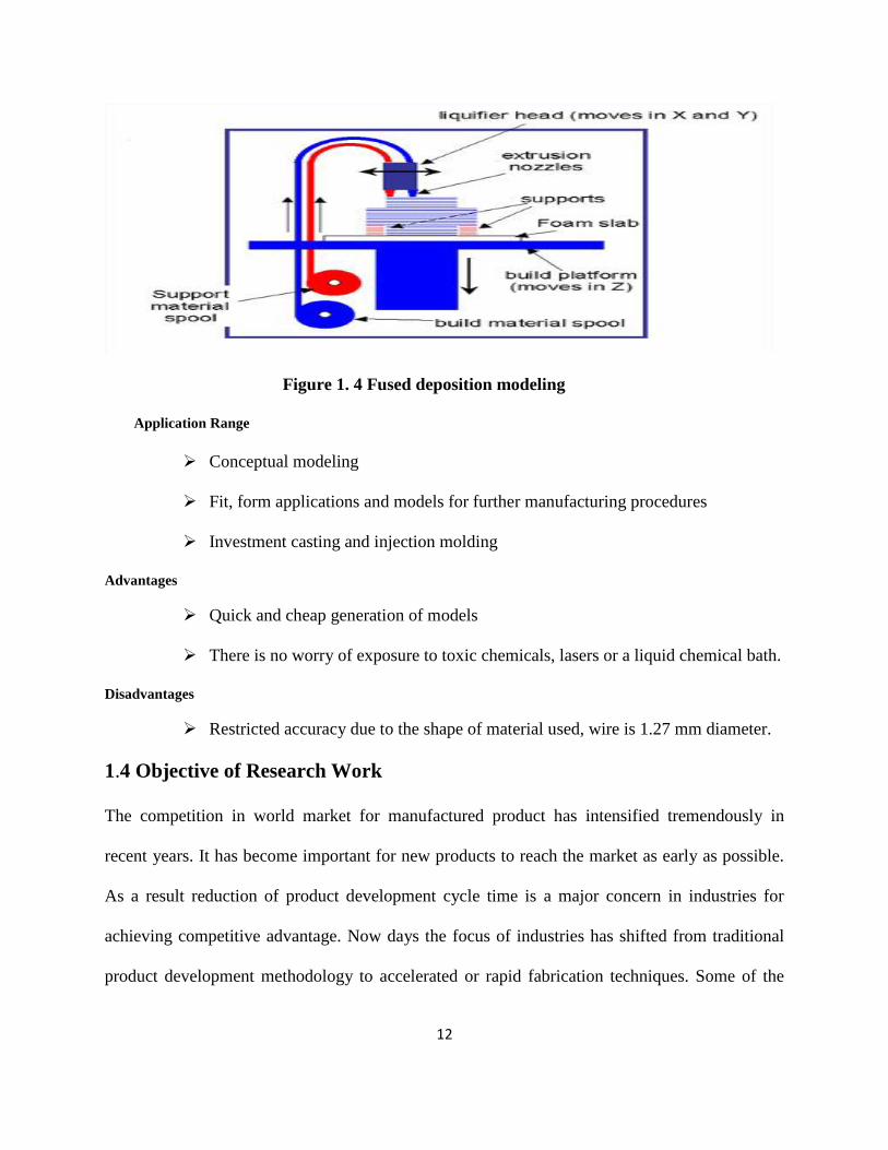
Figure 1. 4 Fused deposition modeling

Application Range

Conceptual modeling

Fit, form applications and models for further manufacturing procedures

Investment casting and injection molding

Advantages

Quick and cheap generation of models

There is no worry of exposure to toxic chemicals, lasers or a liquid chemical bath.

Disadvantages

Restricted accuracy due to the shape of material used, wire is 1.27 mm diameter.

1.4 Objective of Research Work

The competition in world market for manufactured product has intensified tremendously in

recent years. It has become important for new products to reach the market as early as possible.

As a result reduction of product development cycle time is a major concern in industries for

achieving competitive advantage. Now days the focus of industries has shifted from traditional

product development methodology to accelerated or rapid fabrication techniques. Some of the

13

latest developments within the automotive industry have shown how emerging rapid prototyping

and manufacturing (RP&M) technologies can be used to reduce lead time in the prototype

development process. The main benefit rapid prototyping (RP) technologies offer as compared to

conventional subtractive and formative manufacturing process is that virtually any complex

geometry can be built in a layer wise manner directly from CAD model of part without the need

for tooling using a nearly fully automated process. This ability to fabricate complex geometry at

no extra cost is virtually unheard in traditional manufacturing, where there is direct link between

cost of component and complexity of design. On the other hand absence of tooling means that

manufacturing inputs are not required in order to design parts and products . For example if RP is

used to manufactured the part which was conventionally manufactured by injection moulding,

considerations for draft angles, ejection pins and gates marks, wall thickness, sharp corners, weld

lines and parting lines is not important for part design. This directly means whatever can be

designed it can be manufactured. That is optimal design can be selected for manufacturing

without considering the feasibility of their production in terms of available manufacturing

technology. Incorporating features such as undercuts, blind holes, screws in process like

injection moulding often requires expensive tooling, extensive tool setups and testing runs and

inevitably leads to undesirable lead times and costs. Also there is a threshold limit for minimum

production level which has to be cross to offset the cost of tooling. This result in high volume

manufacturing to compensate the tooling cost. Whereas the possibility of producing highly

complex, cost effective custom parts is apparent in RP . Another noted advantage of RP is their

ability to produce functional assembly by consolidating sub assemblies into single unit at the

computer aided design (CAD) stage thus reducing the part count, handling time storage

requirement and without considering the mating and fit problem. RP allows the deposition of

14

multiple materials in any location or combination that the designer requires. This has potentially

enormous implications for the functionality and aesthetics that can be designed into parts .

Having such enormous advantages one of the biggest hindrance in the full scale application of

RP technologies is available materials and their properties, which substantially differ from the

properties of generally used materials. To overcome this limitation one approach is to develop

new materials which can be used by RP machines and have properties superior or as par with

conventional materials. Another procedure is to suitably adjust the process parameters for RP

part fabrication for maximum improvement in the properties. Number of researchers contributed

in this second approach. Their works reveal that properties of RP parts are function of various

process related parameters and can be significantly improved with their proper adjustment. Since

mechanical strength is an important requirement for the functional part there is great need to

improve them. With this aim in mind the present study focus on the mechanical properties viz.

tensile, flexural and impact strength of part fabricated using fused deposition modeling (FDM)

technology and derive the quantitative relation between the processing parameters and

mechanical strength so that the mechanical response of the processed part must be predictable

over the allowable range of parameter.

CHAPTER 2

______________________________________________________________________________

A BRIEF LITERATURE REVIEW

15

2. Literature review

Ahn et al. [4] Uses design of experiment method and concluded that the air gap and raster

orientation affect the tensile strength of FDM processes part where as raster width, model

temperature and colour have little effect. They further compare the measured tensile strength of

FDM part processed at different raster angles and air gap with the tensile strength of injection

moulded part. Material use for both type of fabrication is ABSP400. With zero air gap FDM

specimen tensile strength lies between 10%-73% of injection moulded part with maximum at 0°

and minimum at 90° raster orientation with respect to loading direction. But with negative air

gap there is significant increase in strength at respective raster orientation but still it is less than

the injection moulded part. All specimens failed in transverse direction except for specimen

whose alternate layer raster angle varies between 45° and -45°. This type of specimen failed

along the 45° line. Compression test on the specimen build at two different orientations revealed

that this strength is higher than the tensile strength and lies between 80 to 90% of those for

injection moulded part. Also specimen build with axis perpendicular to build table shows less

compressive strength as compared to specimen build with axis parallel to build table. Based on

these observations it was concluded that strength of FDM processed part is anisotropic.

Es Said et al. [5] Study the effect of raster angle on the tensile, bending and impact properties

of FDM ABSP400 part made using FDM1650 machine. There observations indicate that raster

orientation effect the strength as polymer molecules align themselves along the direction of flow.

Also FDM follows phase change for constructing solid model from solid filament extruded from

nozzle tip in semi molten state and solidify in a chamber maintain at particular temperature. As a

16

result volumetric shrinkage takes place which results in weak interlayer bonding and cause

porosity which reduce the load bearing area.

Lee et al. [6] Performed experiments on cylindrical parts made using three RP processes FDM,

3D printer and nano composite deposition (NCDS) to study the effect of build direction on the

compressive properties. Experimental results show that compressive strength is 11.6% higher for

axial FDM specimen as compared to transverse FDM specimen. In 3D printing, diagonal

specimen possesses maximum compressive strength in comparison to axial specimen. For

NCDS, axial specimen showed compressive strength 23.6% higher than that of transverse

specimen. Out of three RP technologies, parts built by NCDS are most affected by the build

direction.

Khan et al. [7] concluded that layer thickness, raster angle and air gap are found to be

significantly affect the elastic performance of the compliant FDM ABS prototype.

Wang et al. [8], in their work, has mentioned that as extruded material from nozzle cools from

its glass transition temperature to chamber temperature inner stresses will develop particularly

due to uneven deposition speed. These inner stresses will cause the inter layer and the intra layer

deformation which will result in cracking, de-lamination or even part fabrication failure. Thus

affect the part strength and size. They propose the mathematical model to study the effect of total

number of layers, stacking section length, and chamber temperature on the above mentioned

deformations. They concluded that as the total number of layers increase deformation will

decrease rapidly but decreasing tendency will become slow after certain number of layers, higher

stacking section lengths will produce large deformations and as chamber temperature will

increase deformation will decrease and become zero at the glass transition temperature of

17

material. Based on these results they propose that material use for part fabrication must have

lower glass transition temperature and linear shrinkage rate. Also the extruded fiber length must

be small.

Bellehumeur et al. [9] experimentally assessed the bond quality between adjacent filaments

and their failure under flexural loading. Experimental results showed that both the envelope

temperature and variations in the convective conditions with in the building chamber have strong

effect on the meso-structure and the overall quality of bond strength. On line measurements of

the cooling temperature profiles reveals that temperature profile of bottom layers rises above the

glass transition temperature followed by rapid decrease as the extrusion head moves away from

the position of placement of thermoset and minimum temperature increase with the number of

layers. Microphotograph of the cross sectional area shows diffusion of adjacent filaments is more

in lower layers as compared to upper layers for the face of specimen with higher number of

layers.

Chou and Zang [10], in their work, simulated the FDM process using finite element analysis

(FEA) and analyzes the effect of tool path patterns on residual stresses and part distortions. At

each layer stress starts to accumulate at the locations of initial deposition and at tool path turning

point. During the deposition process, the residual stress is smallest for most recently activated

elements as compare to earlier activated element. The residual effect on the bottom surface of

each layer corresponds to stress concentration pattern of its bottom layer. For the long raster

pattern stress concentration characteristic is aligned along the length side and along the width

side for the short raster deposition. Thus the maximum stress zone shifts from the center of the

part towards the length side and width side for the long and short raster pattern respectively.

Simulated results are found to be in agreement with experimental results of the distortion in part

18

except the magnitude of distortion is more than the expected and this may be due to simplified

material properties and boundary conditions assumed during simulation.

Above mention work reveals that the mechanical properties of FDM processed part exhibit

anisotropy and are sensitive to the processing parameters that affect the meso-structure and fibre-

to-fibre bond strength. Also un-even heating and cooling cycles due to inherent nature of FDM

build methodology results in stress accumulation in the build part and these stress concentration

regions will also affect the strength. It is also observed that all the researches in FDM strength

modeling is basically devoted to study the effect of processing conditions on the part strength

with no significant effort made to develop the strength model in terms of FDM process

parameters so as to predict in advance the strength of component for practical application.

Anitha et al. [11], in their result, revealed several interesting features of the FDM process

Only the layer thickness is effective to 49.37% at 95% level of significance. But on pooling, it

was found that the layer thickness is effective to 51.57% at 99% level of significance. The other

factors, road width and speed , contributes to 15.57 and 15.83% at 99% level of significance,

respectively. The significance of layer thickness is further strengthened by the correlation

analysis. Which indicates a strong inverse relationship with surface roughness.

According to the S/N analysis, the layer thickness is most effective when it is at level

3(0.3556mm), the road width at level 1(0.537mm) and the speed of deposition at level 3

(200mm).According to this trials , sample 18 was found to give the best results.

Agrawal et al. [12] In this work, the concept of stochastic modelling of tolerances and

clearances has been extended to RP processes. Using the unified approach for RP processes, the

mechanical error in the FD process has been studied. A methodology has been developed to

analyse the mechanical error at the nozzle tip of the FD process for input values of the tolerances

19

and clearances, where the links and hinges are produced on a mass scale. Closed-form

expressions have been derived to find the mechanical error in the coordinates of a point on the

work surface. It is observed that the influence coefficients of the z coordinate of a point on the

work surface have a larger magnitude than those of the x and y coordinates. The three-sigma

bands obtained in tracing a few example curves by the nozzle tip are plotted. The variances and

their sum are listed in a table to show their variation across the work surface.

The overall error is found to vary appreciably across the work surface. The error is minimum at

the front-left end of the work surface and maximum at the rear-right end. The methodology can

be extended for the optimal allocation of tolerances and clearances to reduce the cost of

manufacturing.

Pandey et al. [13] In this research they found Orientation for part deposition is one of the

important factors as it affects average part surface roughness and production time. In the present

work, two objective functions, namely average part surface roughness and build time, are

formulated.

NSGA-II is successfully used to determine a set of pareto optimal solutions for part deposition

orientation for the two contradicting objectives. It can be seen from the results obtained for

different parts that there exist two limiting situations. One is minimum average part surface

roughness with maximum production time and another is minimum production time with

maximum average part surface roughness. The developed system of part deposition orientation

determination also gives a set of intermediate solutions in which any solution can be used

depending upon the pre- ference of user for the two objectives. The present system can be used

for any class of component, which may be a freeform or a regular object.

CHAPTER 3

______________________________________________________________________________

FUSED DEPOSITION MODELLING

AND ABS MATERIAL

20

3. Fused deposition modeling and ABS material

3.1 Fused Deposition Modeling

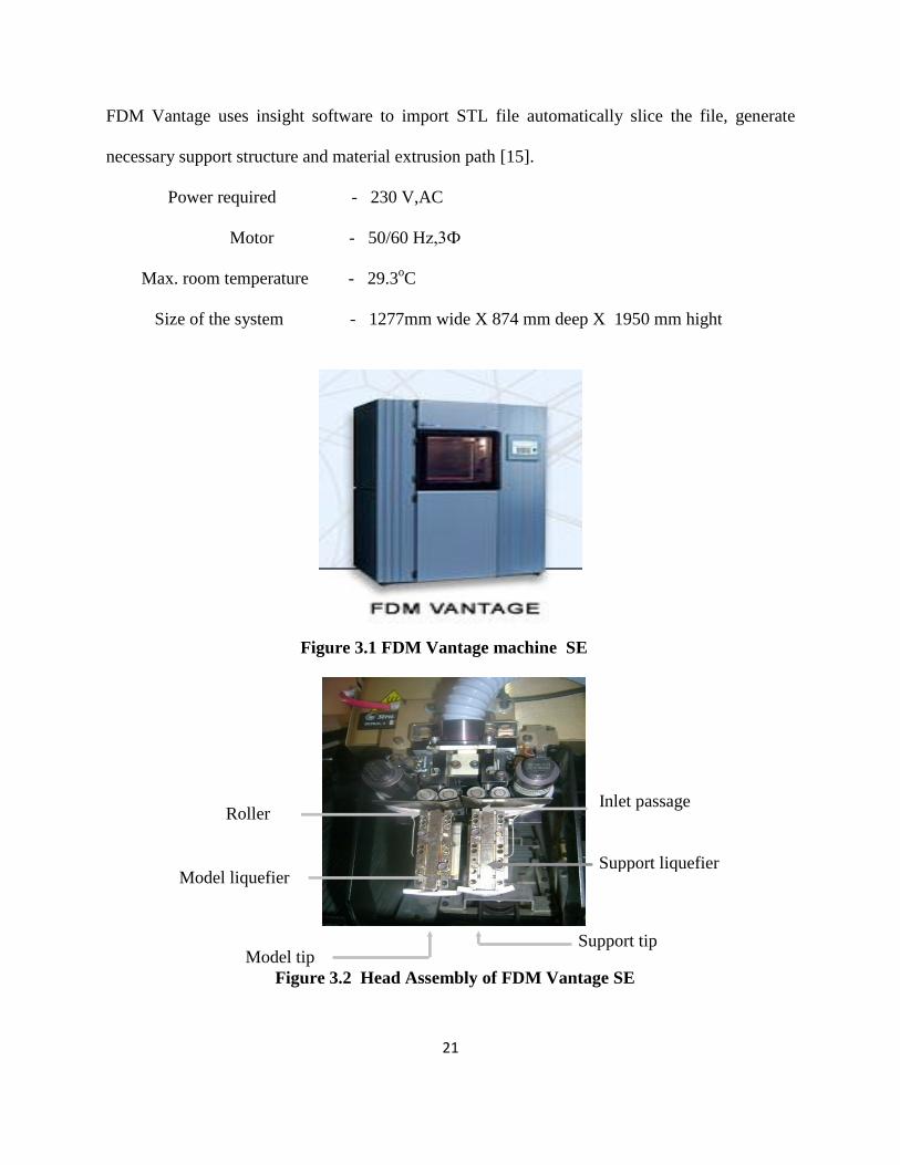
FDM is one of the RP technology developed by Stratasys, USA (Figure 3.1). But unlike other RP

systems which involve an array of lasers, powders, resins, this process uses heated thermoplastic

filaments which are extruded from the tip of nozzle in a temperature controlled environment. For

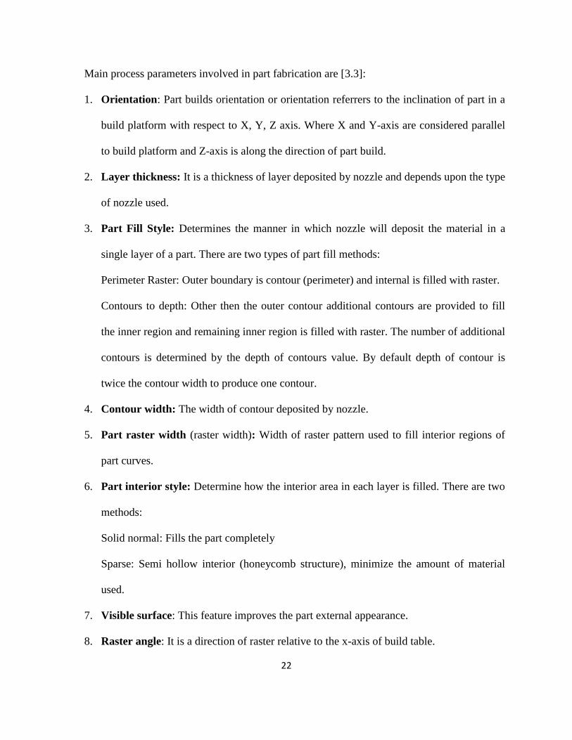
this there is a material deposition subsystem known as head (Figure 3.2) which consist of two

liquefier tips. One tip for model material and other tip for support material deposition both of

which works alternatively. The article forming material is supplied to the head in the form of a

flexible strand of solid material from a supply source (reel). One pair of pulleys or rollers having

a nip in between are utilized as material advance mechanism to grip a flexible strand of modeling

material and advance it into a heated dispensing or liquefier head. The material is heated above

its solidification temperature by a heater on the dispensing head and extruded in a semi molten

state on a previously deposited material onto the build platform following the designed tool path.

The head is attached to the carriage that moves along the X-Y plane. The build platform moves

along the Z direction. The drive motion are provided to selectively move the build platform and

dispensing head relative to each other in a predetermined pattern through drive signals input to

the drive motors from CAD/CAM system. The fabricated part takes the form of a laminate

composite with vertically stacked layers, each of which consists of contiguous material fibres or

rasters with interstitial voids. Fibre-to-fibre bonding within and between layers occurs by a

thermally-driven diffusion bonding process during solidification of the semi-liquid extruded fibre

[14].

21

FDM Vantage uses insight software to import STL file automatically slice the file, generate

necessary support structure and material extrusion path [15].

Power required - 230 V,AC

Motor - 50/60 Hz,3Ф

Max. room temperature - 29.3oC

Size of the system - 1277mm wide X 874 mm deep X 1950 mm hight

Figure 3.1 FDM Vantage machine SE

Figure 3.2 Head Assembly of FDM Vantage SE

Inlet passage Roller

Support liquefier Model liquefier

Support tip Model tip

22

Main process parameters involved in part fabrication are [3.3]:

1. Orientation: Part builds orientation or orientation referrers to the inclination of part in a

build platform with respect to X, Y, Z axis. Where X and Y-axis are considered parallel

to build platform and Z-axis is along the direction of part build.

2. Layer thickness: It is a thickness of layer deposited by nozzle and depends upon the type

of nozzle used.

3. Part Fill Style: Determines the manner in which nozzle will deposit the material in a

single layer of a part. There are two types of part fill methods:

Perimeter Raster: Outer boundary is contour (perimeter) and internal is filled with raster.

Contours to depth: Other then the outer contour additional contours are provided to fill

the inner region and remaining inner region is filled with raster. The number of additional

contours is determined by the depth of contours value. By default depth of contour is

twice the contour width to produce one contour.

4. Contour width: The width of contour deposited by nozzle.

5. Part raster width (raster width): Width of raster pattern used to fill interior regions of

part curves.

6. Part interior style: Determine how the interior area in each layer is filled. There are two

methods:

Solid normal: Fills the part completely

Sparse: Semi hollow interior (honeycomb structure), minimize the amount of material

used.

7. Visible surface: This feature improves the part external appearance.

8. Raster angle: It is a direction of raster relative to the x-axis of build table.

23

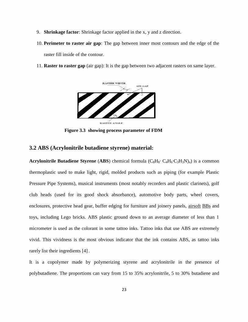
9. Shrinkage factor: Shrinkage factor applied in the x, y and z direction.

10. Perimeter to raster air gap: The gap between inner most contours and the edge of the

raster fill inside of the contour.

11. Raster to raster gap (air gap): It is the gap between two adjacent rasters on same layer.

Figure 3.3 showing process parameter of FDM

3.2 ABS (Acrylonitrile butadiene styrene) material:

Acrylonitrile Butadiene Styrene (ABS) chemical formula (C8H8· C4H6·C3H3N)n) is a common

thermoplastic used to make light, rigid, molded products such as piping (for example Plastic

Pressure Pipe Systems), musical instruments (most notably recorders and plastic clarinets), golf

club heads (used for its good shock absorbance), automotive body parts, wheel covers,

enclosures, protective head gear, buffer edging for furniture and joinery panels, airsoft BBs and

toys, including Lego bricks. ABS plastic ground down to an average diameter of less than 1

micrometer is used as the colorant in some tattoo inks. Tattoo inks that use ABS are extremely

vivid. This vividness is the most obvious indicator that the ink contains ABS, as tattoo inks

rarely list their ingredients [4] .

It is a copolymer made by polymerizing styrene and acrylonitrile in the presence of

polybutadiene. The proportions can vary from 15 to 35% acrylonitrile, 5 to 30% butadiene and

24

40 to 60% styrene. The result is a long chain of polybutadiene criss-crossed with shorter chains

of poly(styrene-co-acrylonitrile). The nitrile groups from neighboring chains, being polar, attract

each other and bind the chains together, making ABS stronger than pure polystyrene. The styrene

gives the plastic a shiny, impervious surface. The butadiene, a rubbery substance, provides

resilience even at low temperatures. ABS can be used between −25 and 60 °C. The properties are

created by rubber toughening, where fine particles of elastomer are distributed throughout the

rigid matrix.

Production of 1 kg of ABS requires the equivalent of about 2 kg of oil for raw materials and

energy. It can also be recycling.

3.3 Properties of ABS plastic

ABS is derived from acrylonitrile, butadiene, and styrene. Acrylonitrile is a synthetic monomer

produced from propylene and ammonia; butadiene is a petroleum hydrocarbon obtained from the

C4 fraction of steam cracking; styrene monomer is made by dehydrogenation of ethyl benzene -

a hydrocarbon obtained in the reaction of ethylene and benzene. The advantage of ABS is that

this material combines the strength and rigidity of the acrylonitrile and styrene polymers with the

toughness of the polybutadiene rubber. The most important mechanical properties of ABS are

resistance and toughness. A variety of modifications can be made to improve impact resistance,

toughness, and heat resistance. The impact resistance can be amplified by increasing the

proportions of polybutadiene in relation to styrene and also acrylonitrile although this causes

changes in other properties. Impact resistance does not fall off rapidly at lower temperatures.

Stability under load is excellent with limited loads [7].

Even though ABS plastics are used largely for mechanical purposes, they also have good

electrical properties that are fairly constant over a wide range of frequencies. These properties

25

are little affected by temperature and atmospheric humidity in the acceptable operating range of

temperatures. The final properties will be influenced to some extent by the conditions under

which the material is processed to the final product; for example, molding at a high temperature

improves the gloss and heat resistance of the product whereas the highest impact resistance and

strength are obtained by molding at low temperature.

ABS polymers are resistant to aqueous acids, alkalis, concentrated hydrochloric and phosphoric

acids, alcohols and animal, vegetable and mineral oils, but they are swollen by glacial acetic

acid, carbon tetrachloride and aromatic hydrocarbons and are attacked by concentrated sulfuric

and nitric acids. They are soluble in esters, ketones and ethylene dichloride.

The aging characteristics of the polymers are largely influenced by the polybutadiene content,

and it is normal to include antioxidants in the composition. On the other hand, while the cost of

producing ABS is roughly twice the cost of producing polystyrene, ABS is considered superior

for its hardness, gloss, toughness, and electrical insulation properties. However, it will be

degraded (dissolve) when exposed to acetone. ABS is flammable when it is exposed to high

temperatures, such as a wood fire. It will "boil", then burst spectacularly into intense, hot flames.

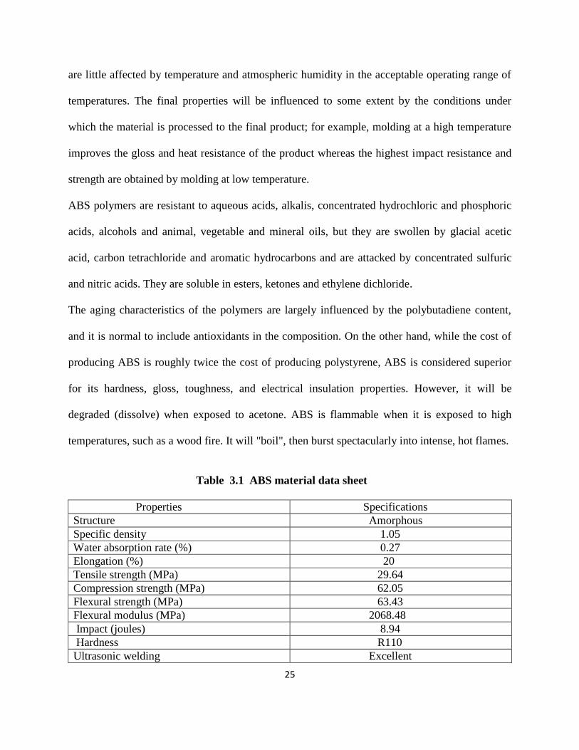
Table 3.1 ABS material data sheet

Properties Specifications

Structure Amorphous

Specific density 1.05

Water absorption rate (%) 0.27

Elongation (%) 20

Tensile strength (MPa) 29.64

Compression strength (MPa) 62.05

Flexural strength (MPa) 63.43

Flexural modulus (MPa) 2068.48

Impact (joules) 8.94

Hardness R110

Ultrasonic welding Excellent

26

Bonding Excellent

Machining Good

Min. utilization temperature (deg. C) -40

Max. utilization temperature (deg .C) 90

Melting point (deg.C) 105

Coefficient of expansion 0.000053

Arc resistance 80

Dielectric strength (KV/mm) 16

Transparency Translucent

UV Resistance Poor

Chemical resistance Good

CHAPTER 4

______________________________________________________________________________

RESPONSE SURFACE METHODOLOGY

27

4. Response surface methodology

Response surface methodology is very useful and modern technique for the prediction and

optimization of machining performances. In the present study, the strength of ABS material part

made by fused deposition modelling machine has been predicted and also process parameters

have been optimized by RSM. In this chapter, overview of RSM has been discussed. Response

surface methodology (RSM) is a collection of statistical and mathematical techniques useful for

developing, improving, and optimizing processes. The most extensive applications of RSM are

in the particular situations where several input variable potentially influence some performance

measure or quality characteristic of the process. This performance measure or quality

characteristic is called the response. The input variables are sometimes called independent

variables. The field of response surface methodology consists of the experimental strategy for

exploring the space of the process or independent variables, Empirical statistical modelling to

develop an approximated relationship between the yield and the process variables. Also, with the

help of response surface methodology, optimization can be done for finding the values of the

process variables that produce desirable values of the response [16].

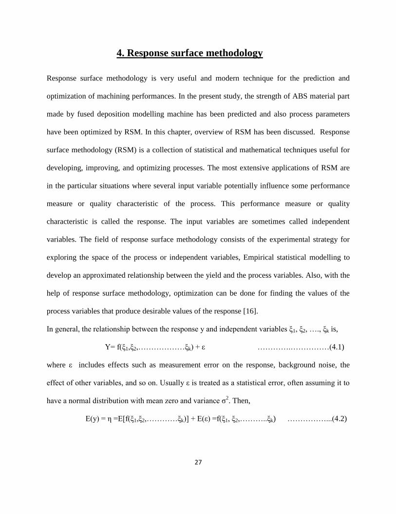
In general, the relationship between the response y and independent variables ξ1, ξ2, …., ξk is,

Y= f(ξ1,ξ2,………………ξk) + ε ………….……………(4.1)

where ε includes effects such as measurement error on the response, background noise, the

effect of other variables, and so on. Usually ε is treated as a statistical error, often assuming it to

have a normal distribution with mean zero and variance σ2. Then,

E(y) = η =E[f(ξ1,ξ2,…………ξk)] + E(ε) =f(ξ1, ξ2,………..ξk) ……………...(4.2)

28

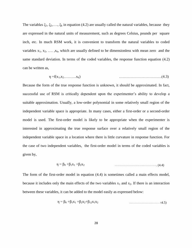
The variables ξ1, ξ2,…., ξk in equation (4.2) are usually called the natural variables, because they

are expressed in the natural units of measurement, such as degrees Celsius, pounds per square

inch, etc. In much RSM work, it is convenient to transform the natural variables to coded

variables x1, x2, …. ,xk, which are usually defined to be dimensionless with mean zero and the

same standard deviation. In terms of the coded variables, the response function equation (4.2)

can be written as,

η =f(x1,x2……….xk) …………………………….(4.3)

Because the form of the true response function is unknown, it should be approximated. In fact,

successful use of RSM is critically dependent upon the experimenter’s ability to develop a

suitable approximation. Usually, a low-order polynomial in some relatively small region of the

independent variable space is appropriate. In many cases, either a first-order or a second-order

model is used. The first-order model is likely to be appropriate when the experimenter is

interested in approximating the true response surface over a relatively small region of the

independent variable space in a location where there is little curvature in response function. For

the case of two independent variables, the first-order model in terms of the coded variables is

given by,

η = β0 +β1x1 +β2x2 …………………………….…………….. (4.4)

The form of the first-order model in equation (4.4) is sometimes called a main effects model,

because it includes only the main effects of the two variables x1 and x2. If there is an interaction

between these variables, it can be added to the model easily as expressed below:

η = β0 +β1x1 +β2x2+β12x1x2 ……………………….……… (4.5)

29

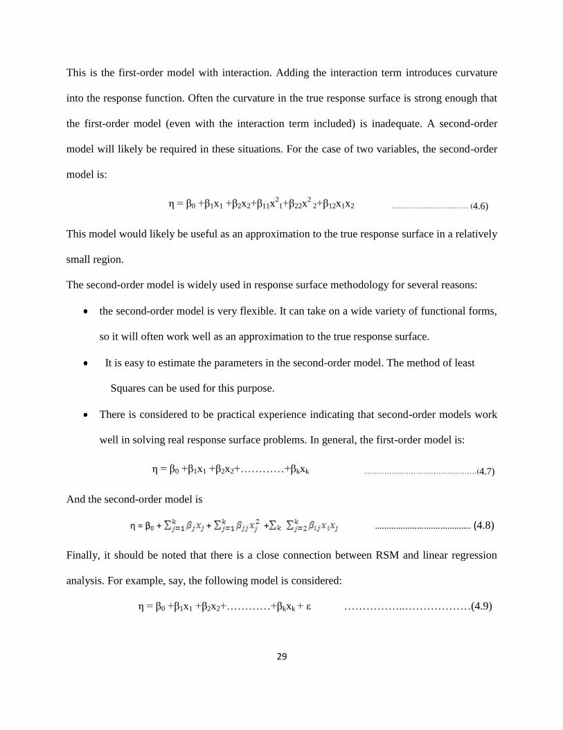
This is the first-order model with interaction. Adding the interaction term introduces curvature

into the response function. Often the curvature in the true response surface is strong enough that

the first-order model (even with the interaction term included) is inadequate. A second-order

model will likely be required in these situations. For the case of two variables, the second-order

model is:

η = β0 +β1x1 +β2x2+β11x21+β22x

2 2+β12x1x2 ……………………..…… (4.6)

This model would likely be useful as an approximation to the true response surface in a relatively

small region.

The second-order model is widely used in response surface methodology for several reasons:

the second-order model is very flexible. It can take on a wide variety of functional forms,

so it will often work well as an approximation to the true response surface.

It is easy to estimate the parameters in the second-order model. The method of least

Squares can be used for this purpose.

There is considered to be practical experience indicating that second-order models work

well in solving real response surface problems. In general, the first-order model is:

η = β0 +β1x1 +β2x2+…………+βkxk …………………………….…………(4.7)

And the second-order model is

η = β0 + + + ………………….………………. (4.8)

Finally, it should be noted that there is a close connection between RSM and linear regression

analysis. For example, say, the following model is considered:

η = β0 +β1x1 +β2x2+…………+βkxk + ε ……………..………………(4.9)

30

The β’s are a set of unknown parameters. To estimate the values of these parameters, the

experimental data must be needed.

4.1. Response Surface Methodology and Robust Design:

RSM is an important branch of experimental design. It is also a critical technology in developing

new processes and optimizing their performance. The objectives of quality improvement,

including reduction of variability and improved process and product performance, can often be

accomplished directly using RSM. It is well known that variation in key performance

characteristics can result in poor process and product quality. During the 1980s, considerable

attention was given to process quality, and methodology was developed for using experimental

design, specifically for the following:

For designing or developing products and processes so that they are robust to component

variation.

For minimizing variability in the output response of a product or a process around a

target value.

For designing products and processes so that they are robust to environment conditions.

By robust means that the product or process performs consistently on target and is

relatively insensitive to factors that are difficult to control.

Professor Genichi Taguchi used the term robust parameter design (RPD) to describe his

approach to this important problem. Essentially, robust parameter design prefers to reduce

process or product variation by choosing levels of controllable factors (or parameters) that make

the system insensitive (or robust) to changes in a set of uncontrollable factors. These

uncontrollable factors represent most of the sources of variability. Taguchi referred to these

uncontrollable factors as noise factors. In RSM, it is assumed that these noise factors are

31

uncontrollable in the field, but can be controlled during process development for purposes of a

designed experiment.

Considerable attention has been focused on the methodology advocated by Taguchi, and a

number of flaws in his approach have been discovered. However, the framework of response

surface methodology allows easily incorporate many useful concepts in his philosophy.

4.2 The Sequential Nature of the Response Surface Methodology:

Most applications of RSM are sequential in nature. They are briefly discussed below:

Phase 0: At first, some ideas should be generated concerning which factors or variables are

likely to be important in response surface study. It is usually known as a screening experiment.

The objective of factor screening is to reduce the list of candidate variables to a relatively few so

that subsequent experiments will be more efficient and require fewer runs or tests. The purpose

of this phase is the identification of the important independent variables.

Phase 1: The objective of the experiment is to determine if the current settings of the

independent variables result in a value of the response that is near the optimum. If the current

settings or levels of the independent variables are not consistent with optimum performance, then

a set of adjustments must be done to the process variables that will move the process toward the

optimum. This phase of RSM makes considerable use of the first-order model and an

optimization technique called the method of steepest ascent /descent.

Phase 2: When the process is near the optimum, it is required to develop a model that will

accurately approximate the true response function within a relatively small region around the

optimum. As the true response surface usually exhibits curvature near the optimum, a second-

order model (or perhaps some higher-order polynomial) should be used. Once an appropriate

approximated model has been obtained, this model may be analyzed to determine the optimum

32

conditions for the process. This sequential experimental process is usually performed within

some region of the independent variable space called the operability region or experimentation

region or region of interest.

4.3 Building Empirical Models:

4.3.1 Linear regression model:

In the practical application of RSM, it is necessary to develop an approximated model for the

true response surface. The true response surface is typically driven by some unknown physical

mechanism. The approximated model is based on observed data from the process or system and

it is an empirical model. Multiple regressions is a collection of statistical techniques useful for

building the types of empirical models required in RSM.

The first-order multiple linear regression models with two independent variables is:

Y = β0+β1x1+β2x2+ε ………………………….………………….(4.10)

The independent variables are often called predictor variables or regressors. The term “linear” is

used because equation (4.10) is a linear function of the unknown parameters β0, β1 and β2.

In general, the response variable y may be related to k regressor variables. The model is given

by:

Y = β0+β1x1+β2x2 +……..+ βkxk+ε ………………………………..(4.11)

This is called a multiple linear regression model with k regressor variables. The parameters

βj, j=0,l, ...k, are called the regression coefficients. Models those are more complex in

appearance than equation (4.11) may often be analyzed by multiple linear regression techniques.

For example, adding an interaction term to the first-order model in two variables, the model

becomes:

Y= βo+β1x1+β2x2+β12x1x2+ε ……………………..………………(4.12)

33

As another example, considering the second-order response surface model in two variables,

the model becomes:

η = β0 +β1x1 +β2x2+β11x21+β22x

2 2+β12x1x2 + ε ……………………(4.13)

In general, any regression model that is linear in the parameters (the β-values) is a linear

regression model, regardless of the shape of the response surface that it generates.

4.3.2 Estimation of the parameters in linear regression models:

The method of least squares is typically used to estimate the regression coefficients in a multiple

linear regression model. It is, say, supposed that n > k observations on the response variable are

available: y1, y2,…., yn. Along with each observed response yi, each regressor variable has to be

observed, xij denotes the i-th observation or level of variable xj. The model in terms of the

observations may be written in matrix notation as:

y = Xβ + ε ……………………………………(4.14)

Where,

y is an n x 1 vector of the observations,

X is an n x p matrix of the levels of the independent variables,

β is a p x 1 vector of the regression coefficients, and

ε is an n x 1 vector of random errors.

It is required to find the vector of least squares estimators, b, that minimizes:

L = ε12 = ε’ε = (y-Xβ)’(y-Xβ) …………………….………....(4.15)

After some simplifications, the least squares estimator of β is:

b= (x’x) -1

x’y …………………………………(4.16)

It is easy to see that X’X is a p x p symmetric matrix and X’y is a p x 1 column vector. The

matrix X’X has the special structure. The diagonal elements of X’X are the sums of squares of

34

the elements in the columns of X, and the off-diagonal elements are the sums of cross-products

of the elements in the columns of X. Furthermore, the elements of X’y are the sums of cross-

products of the columns of X and the observations {yi}.

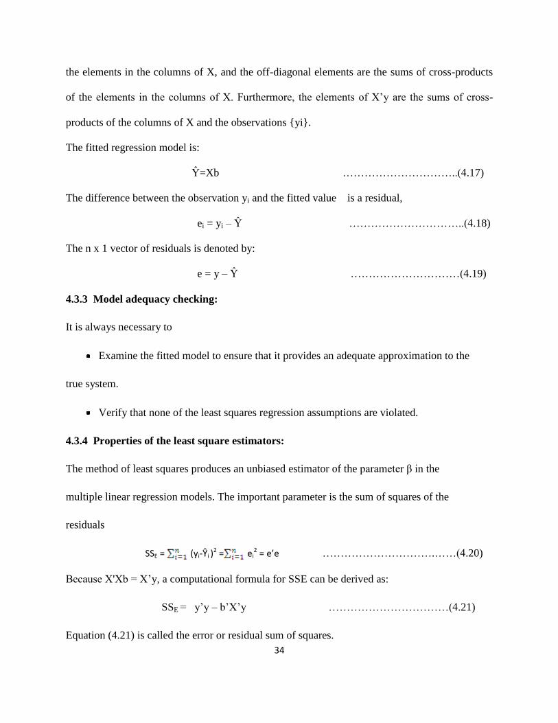
The fitted regression model is:

Ŷ=Xb …………………………..(4.17)

The difference between the observation yi and the fitted value is a residual,

ei = yi – Ŷ …………………………..(4.18)

The n x 1 vector of residuals is denoted by:

e = y – Ŷ …………………………(4.19)

4.3.3 Model adequacy checking:

It is always necessary to

Examine the fitted model to ensure that it provides an adequate approximation to the

true system.

Verify that none of the least squares regression assumptions are violated.

4.3.4 Properties of the least square estimators:

The method of least squares produces an unbiased estimator of the parameter β in the

multiple linear regression models. The important parameter is the sum of squares of the

residuals

SSE = (yi-Ŷi )2 = ei

2 = e’e ………………………….……(4.20)

Because X'Xb = X’y, a computational formula for SSE can be derived as:

SSE = y’y – b’X’y ……………………………(4.21)

Equation (4.21) is called the error or residual sum of squares.

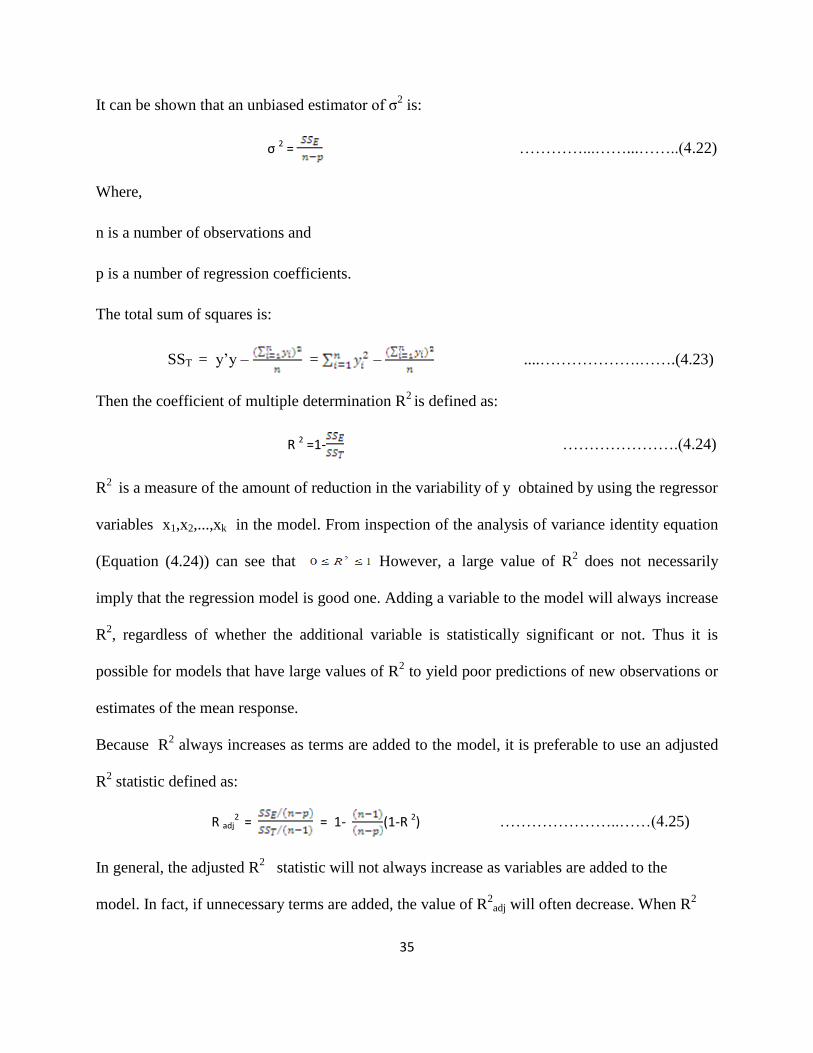
35

It can be shown that an unbiased estimator of σ2 is:

σ 2 = …………...……...……..(4.22)

Where,

n is a number of observations and

p is a number of regression coefficients.

The total sum of squares is:

SST = y’y – = – ....……………….…….(4.23)

Then the coefficient of multiple determination R2 is defined as:

R 2 =1- ………………….(4.24)

R2

is a measure of the amount of reduction in the variability of y obtained by using the regressor

variables x1,x2,...,xk in the model. From inspection of the analysis of variance identity equation

(Equation (4.24)) can see that However, a large value of R2 does not necessarily

imply that the regression model is good one. Adding a variable to the model will always increase

R2, regardless of whether the additional variable is statistically significant or not. Thus it is

possible for models that have large values of R2 to yield poor predictions of new observations or

estimates of the mean response.

Because R2 always increases as terms are added to the model, it is preferable to use an adjusted

R2 statistic defined as:

R adj2 = = 1- (1-R 2) …………………..……(4.25)

In general, the adjusted R2 statistic will not always increase as variables are added to the

model. In fact, if unnecessary terms are added, the value of R2

adj will often decrease. When R2

36

and R2

adj differ dramatically, there is a good chance that non significant terms have been

included in the model.

However, testing hypotheses on the individual regression coefficients are very much important.

Such tests would be useful in determining the value of each of the regressor variables in the

regression model. For example, the model might be more effective with the inclusion of

additional variables, or perhaps with the deletion of one or more of the variables already in the

model.

Adding a variable to the regression model always causes the sum of squares for regression to

increase and the error sum of squares to decrease. It must be decided whether the increase in the

regression sum of squares is sufficient to warrant using the additional variable in the model.

Furthermore, adding an unimportant variable to the model can actually increase the mean square

error, thereby decreasing the usefulness of the model [17].

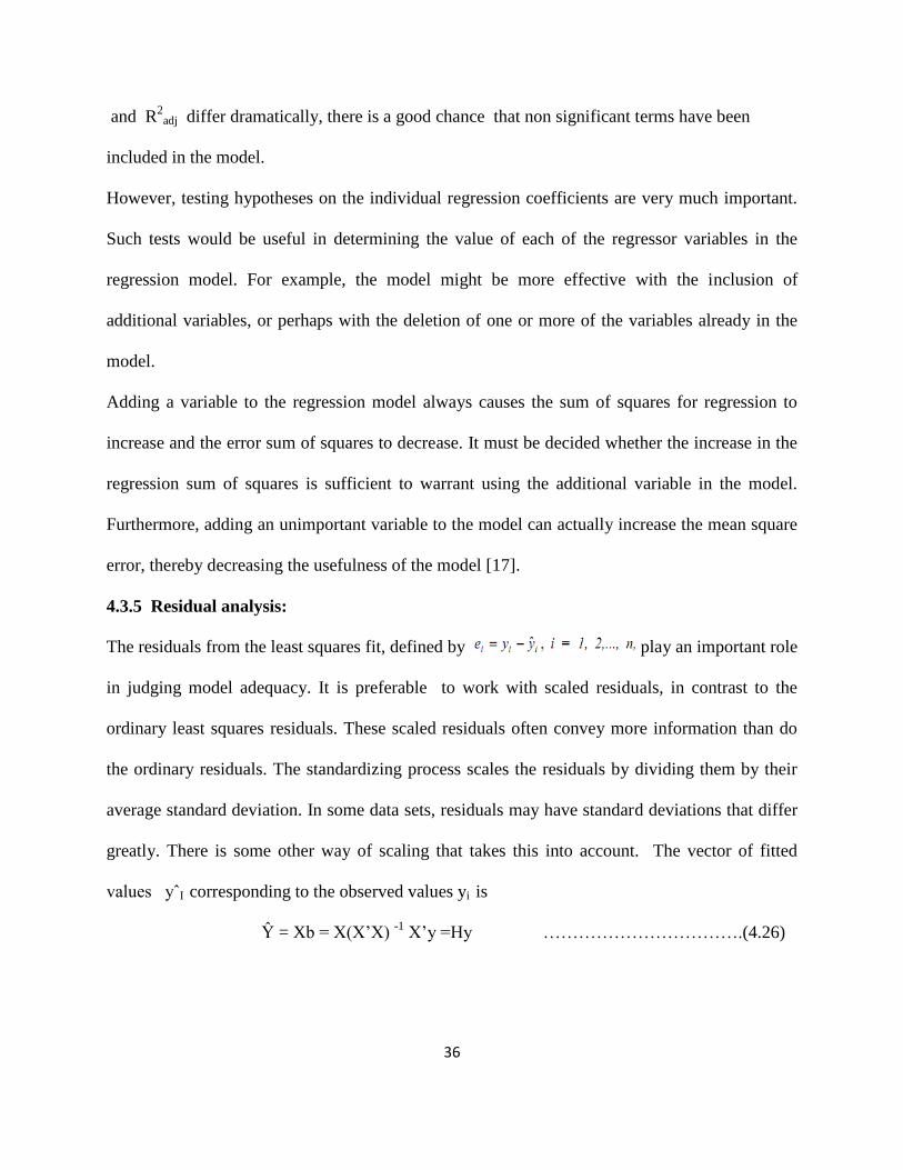
4.3.5 Residual analysis:

The residuals from the least squares fit, defined by play an important role

in judging model adequacy. It is preferable to work with scaled residuals, in contrast to the

ordinary least squares residuals. These scaled residuals often convey more information than do

the ordinary residuals. The standardizing process scales the residuals by dividing them by their

average standard deviation. In some data sets, residuals may have standard deviations that differ

greatly. There is some other way of scaling that takes this into account. The vector of fitted

values yˆI corresponding to the observed values yi is

Ŷ = Xb = X(X’X) -1

X’y =Hy …………………………….(4.26)

37

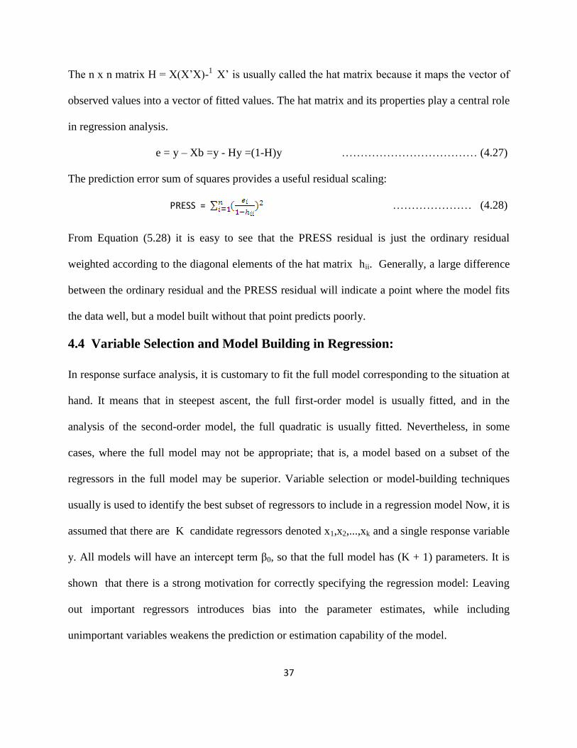
The n x n matrix H = X(X’X)-1

X’ is usually called the hat matrix because it maps the vector of

observed values into a vector of fitted values. The hat matrix and its properties play a central role

in regression analysis.

e = y – Xb =y - Hy =(1-H)y ……………………………… (4.27)

The prediction error sum of squares provides a useful residual scaling:

PRESS = ………………… (4.28)

From Equation (5.28) it is easy to see that the PRESS residual is just the ordinary residual

weighted according to the diagonal elements of the hat matrix hii. Generally, a large difference

between the ordinary residual and the PRESS residual will indicate a point where the model fits

the data well, but a model built without that point predicts poorly.

4.4 Variable Selection and Model Building in Regression:

In response surface analysis, it is customary to fit the full model corresponding to the situation at

hand. It means that in steepest ascent, the full first-order model is usually fitted, and in the

analysis of the second-order model, the full quadratic is usually fitted. Nevertheless, in some

cases, where the full model may not be appropriate; that is, a model based on a subset of the

regressors in the full model may be superior. Variable selection or model-building techniques

usually is used to identify the best subset of regressors to include in a regression model Now, it is

assumed that there are K candidate regressors denoted x1,x2,...,xk and a single response variable

y. All models will have an intercept term β0, so that the full model has (K + 1) parameters. It is

shown that there is a strong motivation for correctly specifying the regression model: Leaving

out important regressors introduces bias into the parameter estimates, while including

unimportant variables weakens the prediction or estimation capability of the model.

38

4.4.1 Procedures for variable selection:

Now, it is required to find several of the more widely used methods for selecting the appropriate

subset of variables for a regression model. The approach is also made on the optimization

procedure used for selecting the best model from the whole set of models and finally it is

required to discuss and illustrate several of the criteria that are typically used to decide which

subset of the candidate regressors leads to the best model.

4.4.2 All possible regression:

This procedure requires that all the regression equations are fitted involving one-candidate

regressors, two-candidate regressors, and so on. These equations are evaluated according to some

suitable criterion, and the best regression model selected. If it is assumed that the intercept term

β0 is included in all equations, then there are K candidate regressors and there are 2K total

equations to be estimated and examined. For example, if K = 4, then there are 24= 16 possible

equations, whereas if K = 10, then there are210

= 1024. Clearly the number of equations to be

examined increases rapidly as the number of candidate regressors increases. Usually, the

candidate variables are restricted for the model to those in the full quadratic polynomial and it is

required that all models obey the principal of hierarchy. A model is said to be hierarchical if the

presence of higher-order terms (such as interaction and second-order terms) requires the

inclusion of all lower-order terms contained within those of higher order. For example, this

would require the inclusion of both main effects, if a two-factor interaction term was in the

model. Many regression model builders believe that hierarchy is a reasonable model-building

practice while fitting polynomials.

39

4.4.3 Stepwise regression methods:

As the evaluation of all possible regressions can be burdensome, various methods have been

developed for evaluating only a small number of subset regression models by either adding or

deleting regressors one at a time. These methods are generally referred to as stepwise-type

procedures. They can be classified into three broad categories:

a) Forward selection,

b) Backward elimination, and

c) Stepwise regression, which is a popular combination of procedures (a) and (b).

a) Forward selection:

This procedure begins with the assumption that there are no regressors in the model other than

the intercept. An effort is made to find an optimal subset by inserting regressors into the model

one at a time. The first regressor selected for entry into the equation is the one that has the largest

simple correlation with the response variable y. If it is supposed that the first regressor is x1, then

the regressor will produce the largest value of the F-statistic for testing significance of

regression. This regressor is entered, if the F-statistic exceeds a pre-selected F-value, say, Fin (or

F-to-enter). The second regressor chosen for entry is the one that now has the largest correlation

with y after adjusting for the effect of the first regressor entered (x1) on y. It is referred as partial

correlations. In general, at each step the regressor having the highest partial correlation with y (or

equivalently the largest partial F-statistic given the other regressors already in the model) is

added to the model, if its partial F-statistic exceeds the pre-selected entry level Fin. The

procedure terminates either when the partial F-statistic at a particular step does not exceed Fin or

when the last candidate regressor is added to the model.

40

b) Backward elimination:

Forward selection begins with no regressors in the model and attempts to insert variables until a

suitable model is obtained. Backward elimination attempts to find a good model by working in

the opposite direction. That is, it is required to start a model that includes all K Candidate

regressors. Then the partial F-statistic (or a t-statistic, which is equivalent) is computed for each

regressor, as if, it were the last variable to enter the model. The smallest of these partial F-

statistics is compared with a pre-selected value, Fout (or F-to-remove); and if the smallest partial

F-value is less than Fout, that regressor is removed from the model. Now, a regression model with

(K – 1) regressors is fitted, the partial F-statistic for this new model calculated, and the procedure

repeated. The backward elimination algorithm terminates, when the smallest partial F-value is

not less than the pre-selected cut-off value Fout.

c) Stepwise regression:

The two procedures described above suggest a number of possible combinations. One of the

most popular is the stepwise regression algorithm. This is a modification of forward selection in

which at each step all regressors, entered into the model previously, are reassessed via their

partial F-or t-statistics. A regressor added at an earlier step may now be redundant because of the

relationship between it and regressors now in the equation. If the partial F-statistic for a variable

is less than Fout, that variable is dropped from the model. Stepwise regression requires two cut-

off values, Fin and Fout. Sometimes, it is preferred to choose Fin = Fout, although this is not

necessary. Sometimes, it is also chosen that Fin > Fout, making it more difficult to add a regressor

than to delete one. In the present study, some of the concepts of RSM have been used for

predicting the FDM response viz, Tensile Strength, Flexural strength, and Impact strength. Also,

the optimization of process parameters has been done by RSM.

CHAPTER 5

______________________________________________________________________________

SPECIMEN PREPARATION,

EXPERIMENT AND ANALYS

41

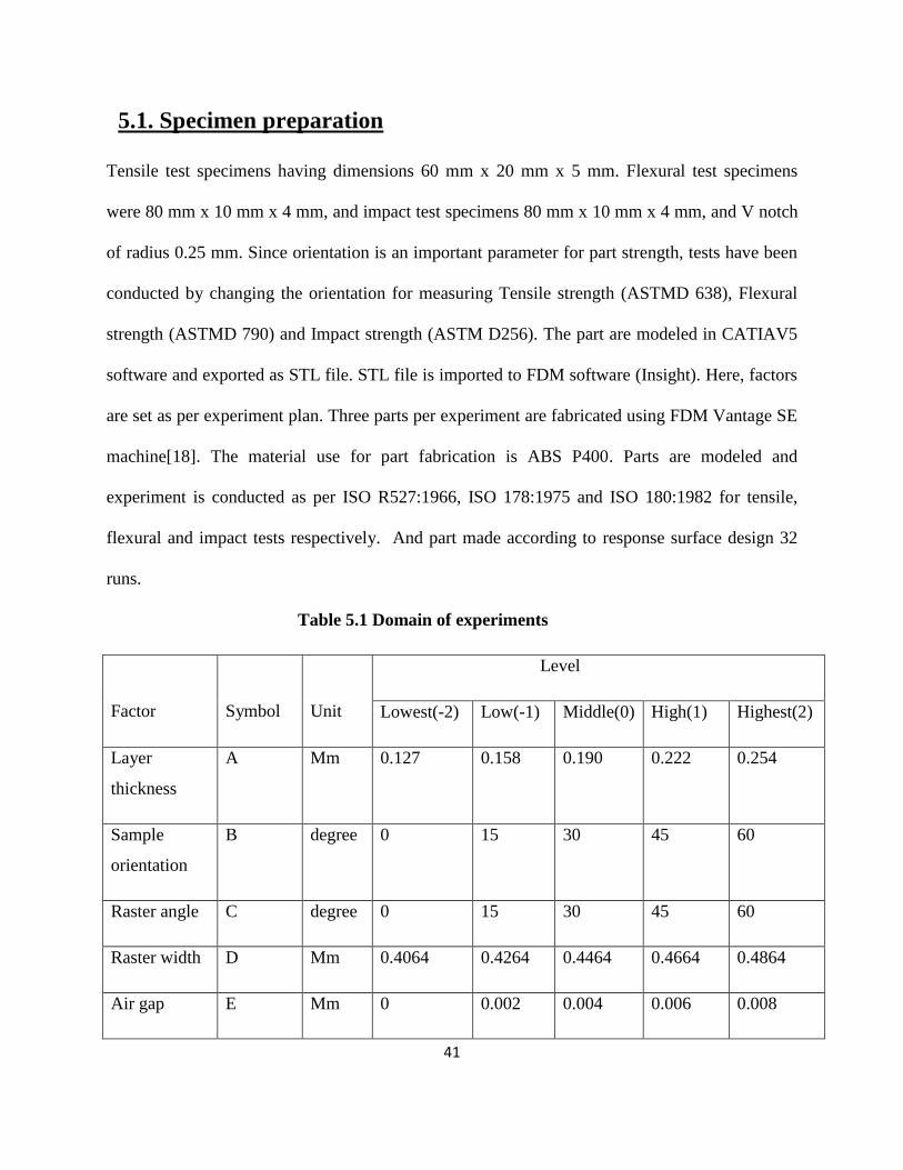
5.1. Specimen preparation

Tensile test specimens having dimensions 60 mm x 20 mm x 5 mm. Flexural test specimens

were 80 mm x 10 mm x 4 mm, and impact test specimens 80 mm x 10 mm x 4 mm, and V notch

of radius 0.25 mm. Since orientation is an important parameter for part strength, tests have been

conducted by changing the orientation for measuring Tensile strength (ASTMD 638), Flexural

strength (ASTMD 790) and Impact strength (ASTM D256). The part are modeled in CATIAV5

software and exported as STL file. STL file is imported to FDM software (Insight). Here, factors

are set as per experiment plan. Three parts per experiment are fabricated using FDM Vantage SE

machine[18]. The material use for part fabrication is ABS P400. Parts are modeled and

experiment is conducted as per ISO R527:1966, ISO 178:1975 and ISO 180:1982 for tensile,

flexural and impact tests respectively. And part made according to response surface design 32

runs.

Table 5.1 Domain of experiments

Factor

Symbol

Unit

Level

Lowest(-2) Low(-1) Middle(0) High(1) Highest(2)

Layer

thickness

A Mm 0.127 0.158 0.190 0.222 0.254

Sample

orientation

B degree 0 15 30 45 60

Raster angle C degree 0 15 30 45 60

Raster width D Mm 0.4064 0.4264 0.4464 0.4664 0.4864

Air gap E Mm 0 0.002 0.004 0.006 0.008

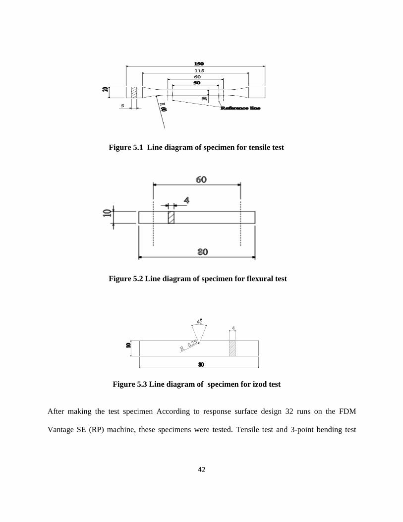
42

Figure 5.1 Line diagram of specimen for tensile test

Figure 5.2 Line diagram of specimen for flexural test

Figure 5.3 Line diagram of specimen for izod test

After making the test specimen According to response surface design 32 runs on the FDM

Vantage SE (RP) machine, these specimens were tested. Tensile test and 3-point bending test

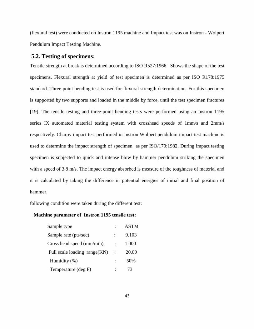
43

(flexural test) were conducted on Instron 1195 machine and Impact test was on Instron - Wolpert

Pendulum Impact Testing Machine.

5.2. Testing of specimens:

Tensile strength at break is determined according to ISO R527:1966. Shows the shape of the test

specimens. Flexural strength at yield of test specimen is determined as per ISO R178:1975

standard. Three point bending test is used for flexural strength determination. For this specimen

is supported by two supports and loaded in the middle by force, until the test specimen fractures

[19]. The tensile testing and three-point bending tests were performed using an Instron 1195

series IX automated material testing system with crosshead speeds of 1mm/s and 2mm/s

respectively. Charpy impact test performed in Instron Wolpert pendulum impact test machine is

used to determine the impact strength of specimen as per ISO/179:1982. During impact testing

specimen is subjected to quick and intense blow by hammer pendulum striking the specimen

with a speed of 3.8 m/s. The impact energy absorbed is measure of the toughness of material and

it is calculated by taking the difference in potential energies of initial and final position of

hammer.

following condition were taken during the different test:

Machine parameter of Instron 1195 tensile test:

Sample type : ASTM

Sample rate (pts/sec) : 9.103

Cross head speed (mm/min) : 1.000

Full scale loading range(KN) : 20.00

Humidity (%) : 50%

Temperature (deg.F) : 73

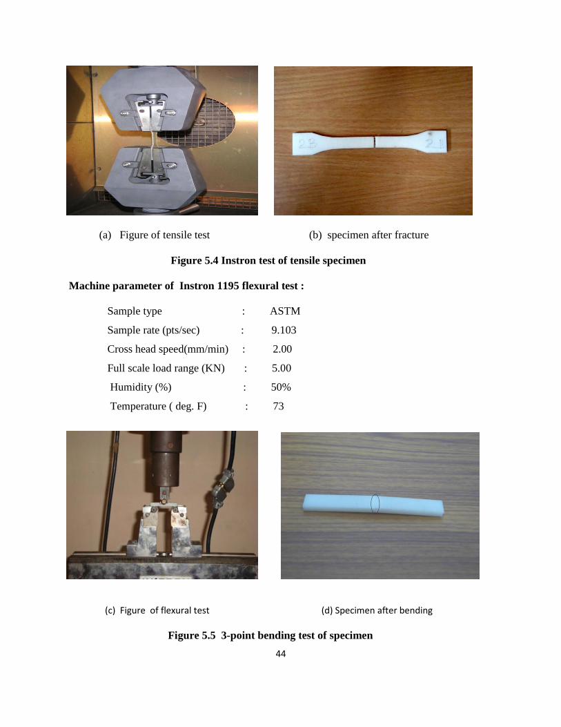
44

(a) Figure of tensile test (b) specimen after fracture

Figure 5.4 Instron test of tensile specimen

Machine parameter of Instron 1195 flexural test :

Sample type : ASTM

Sample rate (pts/sec) : 9.103

Cross head speed(mm/min) : 2.00

Full scale load range (KN) : 5.00

Humidity (%) : 50%

Temperature ( deg. F) : 73

(c) Figure of flexural test (d) Specimen after bending

Figure 5.5 3-point bending test of specimen

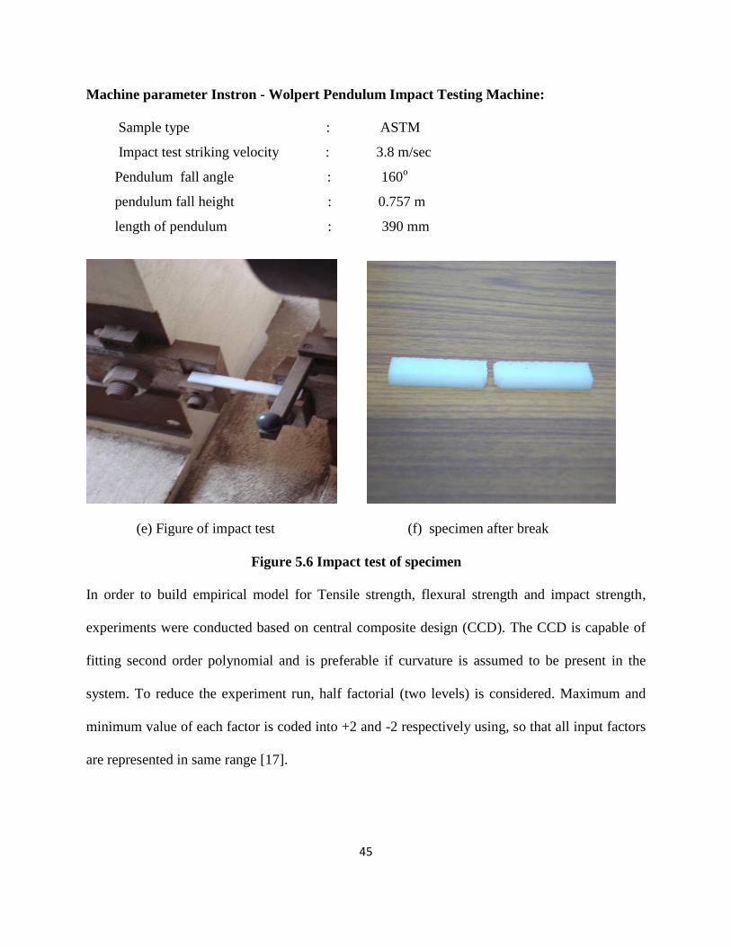
45

Machine parameter Instron - Wolpert Pendulum Impact Testing Machine:

Sample type : ASTM

Impact test striking velocity : 3.8 m/sec

Pendulum fall angle : 160o

pendulum fall height : 0.757 m

length of pendulum : 390 mm

(e) Figure of impact test (f) specimen after break

Figure 5.6 Impact test of specimen

In order to build empirical model for Tensile strength, flexural strength and impact strength,

experiments were conducted based on central composite design (CCD). The CCD is capable of

fitting second order polynomial and is preferable if curvature is assumed to be present in the

system. To reduce the experiment run, half factorial (two levels) is considered. Maximum and

minimum value of each factor is coded into +2 and -2 respectively using, so that all input factors

are represented in same range [17].

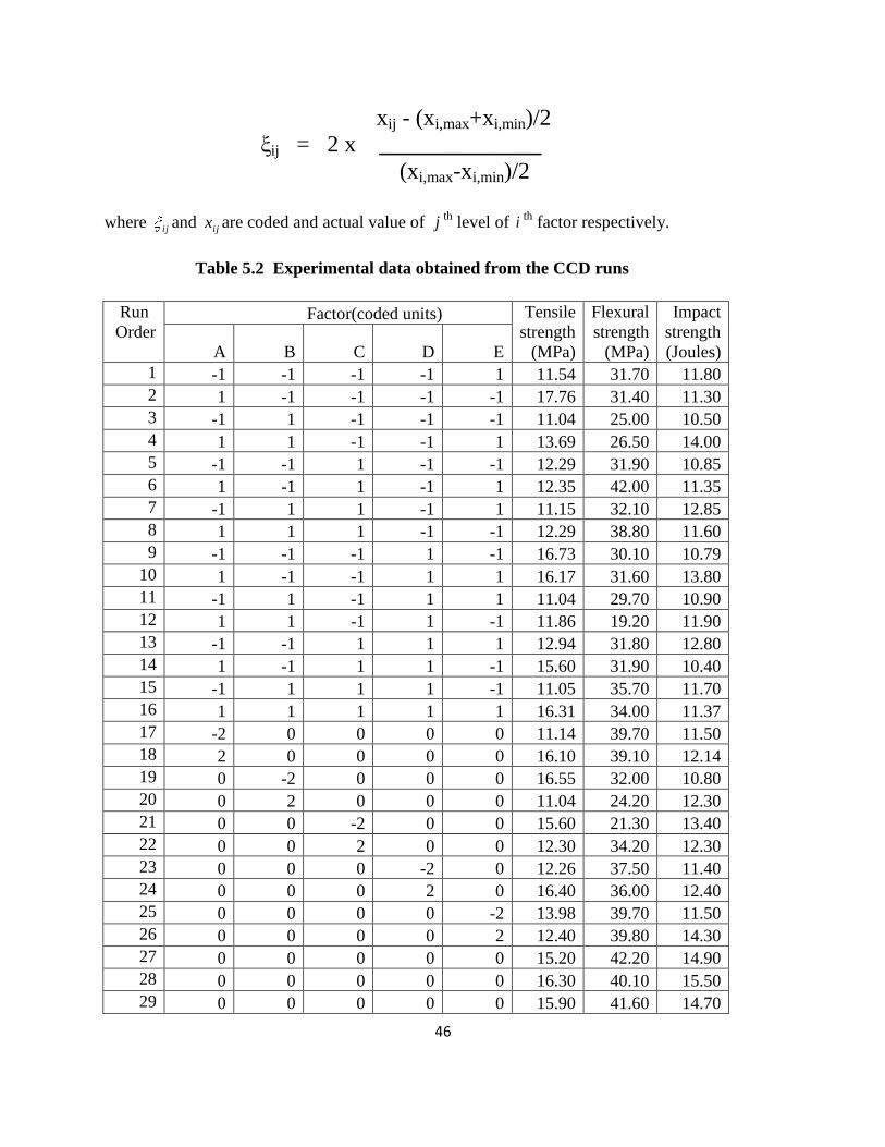
46

xij - (xi,max+xi,min)/2

ξij = 2 x ______________

(xi,max-xi,min)/2

where ij and ijx are coded and actual value of j

th level of i

th factor respectively.

Table 5.2 Experimental data obtained from the CCD runs

Run

Order Factor(coded units) Tensile

strength

(MPa)

Flexural

strength

(MPa)

Impact

strength

(Joules) A B C D E

1 -1 -1 -1 -1 1 11.54 31.70 11.80

2 1 -1 -1 -1 -1 17.76 31.40 11.30

3 -1 1 -1 -1 -1 11.04 25.00 10.50

4 1 1 -1 -1 1 13.69 26.50 14.00

5 -1 -1 1 -1 -1 12.29 31.90 10.85

6 1 -1 1 -1 1 12.35 42.00 11.35

7 -1 1 1 -1 1 11.15 32.10 12.85

8 1 1 1 -1 -1 12.29 38.80 11.60

9 -1 -1 -1 1 -1 16.73 30.10 10.79

10 1 -1 -1 1 1 16.17 31.60 13.80

11 -1 1 -1 1 1 11.04 29.70 10.90

12 1 1 -1 1 -1 11.86 19.20 11.90

13 -1 -1 1 1 1 12.94 31.80 12.80

14 1 -1 1 1 -1 15.60 31.90 10.40

15 -1 1 1 1 -1 11.05 35.70 11.70

16 1 1 1 1 1 16.31 34.00 11.37

17 -2 0 0 0 0 11.14 39.70 11.50

18 2 0 0 0 0 16.10 39.10 12.14

19 0 -2 0 0 0 16.55 32.00 10.80

20 0 2 0 0 0 11.04 24.20 12.30

21 0 0 -2 0 0 15.60 21.30 13.40

22 0 0 2 0 0 12.30 34.20 12.30

23 0 0 0 -2 0 12.26 37.50 11.40

24 0 0 0 2 0 16.40 36.00 12.40

25 0 0 0 0 -2 13.98 39.70 11.50

26 0 0 0 0 2 12.40 39.80 14.30

27 0 0 0 0 0 15.20 42.20 14.90

28 0 0 0 0 0 16.30 40.10 15.50

29 0 0 0 0 0 15.90 41.60 14.70

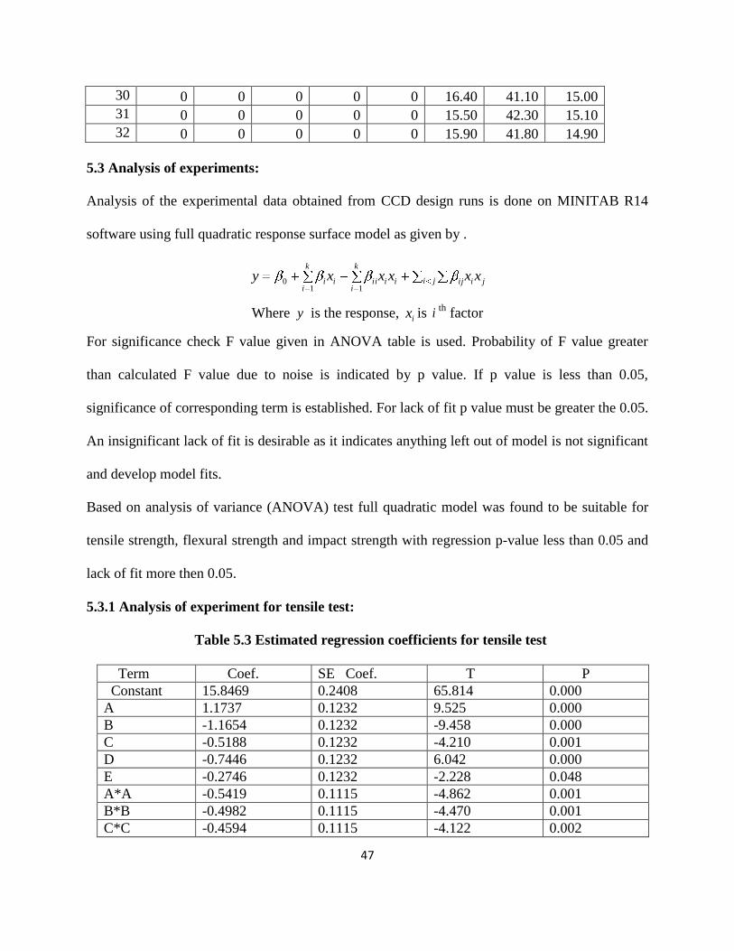
47

30 0 0 0 0 0 16.40 41.10 15.00

31 0 0 0 0 0 15.50 42.30 15.10

32 0 0 0 0 0 15.90 41.80 14.90

5.3 Analysis of experiments:

Analysis of the experimental data obtained from CCD design runs is done on MINITAB R14

software using full quadratic response surface model as given by .

ji jiij

k

iiiii

k

iii xxxxxy

110

Where y is the response, ix is ith

factor

For significance check F value given in ANOVA table is used. Probability of F value greater

than calculated F value due to noise is indicated by p value. If p value is less than 0.05,

significance of corresponding term is established. For lack of fit p value must be greater the 0.05.

An insignificant lack of fit is desirable as it indicates anything left out of model is not significant

and develop model fits.

Based on analysis of variance (ANOVA) test full quadratic model was found to be suitable for

tensile strength, flexural strength and impact strength with regression p-value less than 0.05 and

lack of fit more then 0.05.

5.3.1 Analysis of experiment for tensile test:

Table 5.3 Estimated regression coefficients for tensile test

Term Coef. SE Coef. T P

Constant 15.8469 0.2408 65.814 0.000

A 1.1737 0.1232 9.525 0.000

B -1.1654 0.1232 -9.458 0.000

C -0.5188 0.1232 -4.210 0.001

D -0.7446 0.1232 6.042 0.000

E -0.2746 0.1232 -2.228 0.048

A*A -0.5419 0.1115 -4.862 0.001

B*B -0.4982 0.1115 -4.470 0.001

C*C -0.4594 0.1115 -4.122 0.002

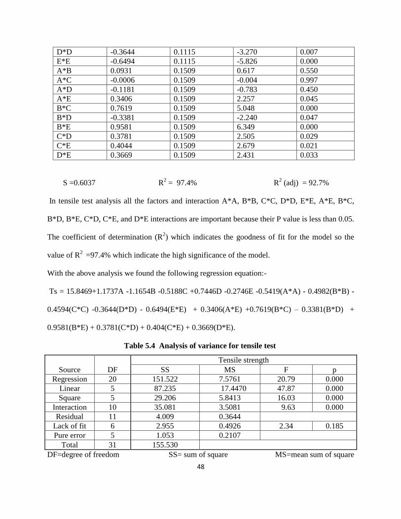
48

D*D -0.3644 0.1115 -3.270 0.007

E*E -0.6494 0.1115 -5.826 0.000

A*B 0.0931 0.1509 0.617 0.550

A*C -0.0006 0.1509 -0.004 0.997

A*D -0.1181 0.1509 -0.783 0.450

A*E 0.3406 0.1509 2.257 0.045

B*C 0.7619 0.1509 5.048 0.000

B*D -0.3381 0.1509 -2.240 0.047

B*E 0.9581 0.1509 6.349 0.000

C*D 0.3781 0.1509 2.505 0.029

C*E 0.4044 0.1509 2.679 0.021

D*E 0.3669 0.1509 2.431 0.033

S =0.6037 R2 = 97.4% R

2 (adj) = 92.7%

In tensile test analysis all the factors and interaction A*A, B*B, C*C, D*D, E*E, A*E, B*C,

B*D, B*E, C*D, C*E, and D*E interactions are important because their P value is less than 0.05.

The coefficient of determination (R2) which indicates the goodness of fit for the model so the

value of R2

=97.4% which indicate the high significance of the model.

With the above analysis we found the following regression equation:-

Ts = 15.8469+1.1737A -1.1654B -0.5188C +0.7446D -0.2746E -0.5419(A*A) - 0.4982(B*B) -

0.4594(C*C) -0.3644(D*D) - 0.6494(E*E) + 0.3406(A*E) +0.7619(B*C) – 0.3381(B*D) +

0.9581(B*E) + 0.3781(C*D) + 0.404(C*E) + 0.3669(D*E).

Table 5.4 Analysis of variance for tensile test

DF=degree of freedom SS= sum of square MS=mean sum of square

Source DF

Tensile strength

SS MS F p

Regression 20 151.522 7.5761 20.79 0.000

Linear 5 87.235 17.4470 47.87 0.000

Square 5 29.206 5.8413 16.03 0.000

Interaction 10 35.081 3.5081 9.63 0.000

Residual 11 4.009 0.3644

Lack of fit 6 2.955 0.4926 2.34 0.185

Pure error 5 1.053 0.2107

Total 31 155.530

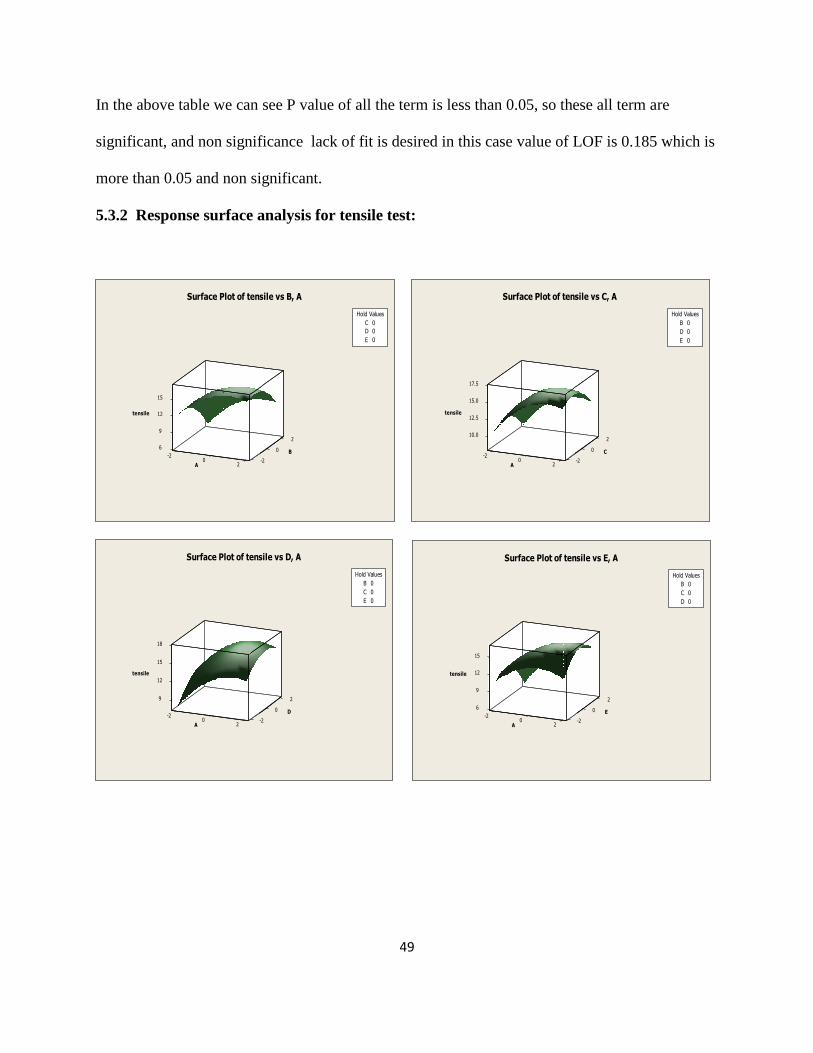
49

In the above table we can see P value of all the term is less than 0.05, so these all term are

significant, and non significance lack of fit is desired in this case value of LOF is 0.185 which is

more than 0.05 and non significant.

5.3.2 Response surface analysis for tensile test:

2

tensile

6

9

0

12

B

15

-20 -2

2A

Hold Values

C 0

D 0

E 0

Surface Plot of tensile vs B, A

2

tensile

10.0

0

12.5

15.0

C

17.5

-20 -2

2A

Hold Values

B 0

D 0

E 0

Surface Plot of tensile vs C, A

2

tensile

9

0

12

D

15

18

-20 -2

2A

Hold Values

B 0

C 0

E 0

Surface Plot of tensile vs D, A

2

tensile

6

9

0

12

E

15

-20 -2

2A

Hold Values

B 0

C 0

D 0

Surface Plot of tensile vs E, A

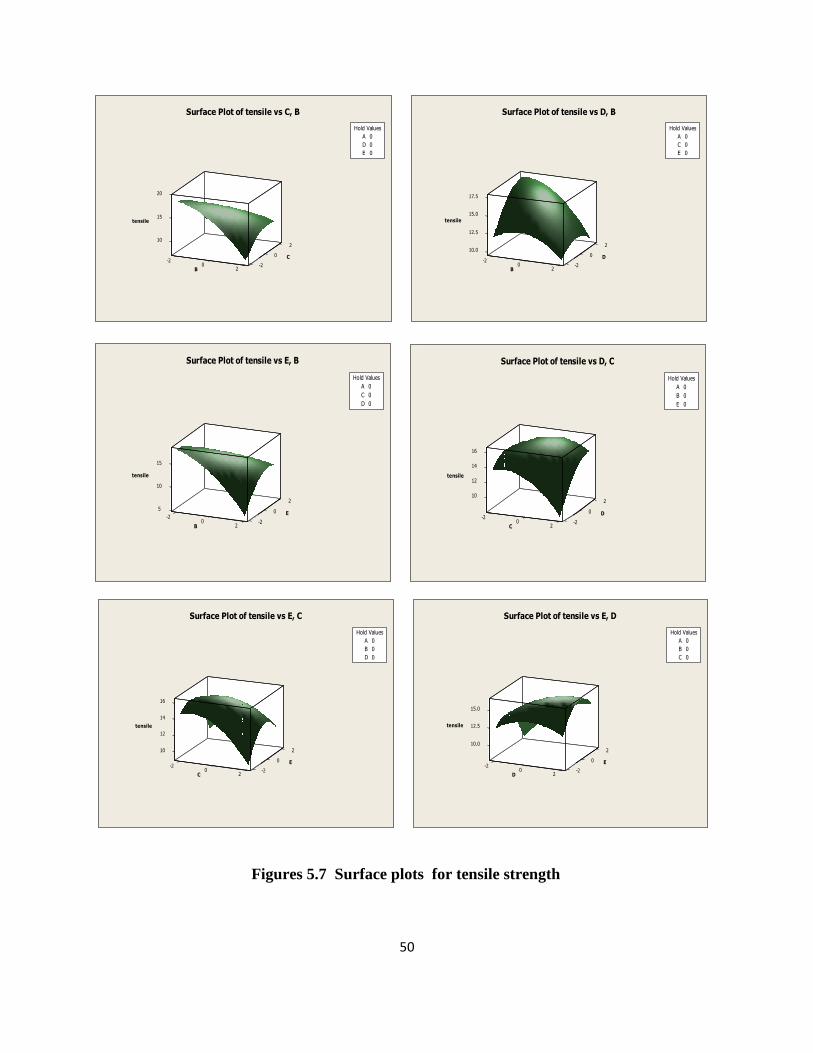
50

2

tensile

10

0

15

C

20

-20 -2

2B

Hold Values

A 0

D 0

E 0

Surface Plot of tensile vs C, B

2

tensile

10.0

12.5

0

15.0

D

17.5

-20 -2

2B

Hold Values

A 0

C 0

E 0

Surface Plot of tensile vs D, B

2

tensile

5 0

10

E

15

-20 -2

2B

Hold Values

A 0

C 0

D 0

Surface Plot of tensile vs E, B

2

tensile

10

0

12

D

14

16

-20 -2

2C

Hold Values

A 0

B 0

E 0

Surface Plot of tensile vs D, C

2

tensile

10

0

12

14

E

16

-20 -2

2C

Hold Values

A 0

B 0

D 0

Surface Plot of tensile vs E, C

2

tensile

10.0

0

12.5

E

15.0

-20 -2

2D

Hold Values

A 0

B 0

C 0

Surface Plot of tensile vs E, D

Figures 5.7 Surface plots for tensile strength

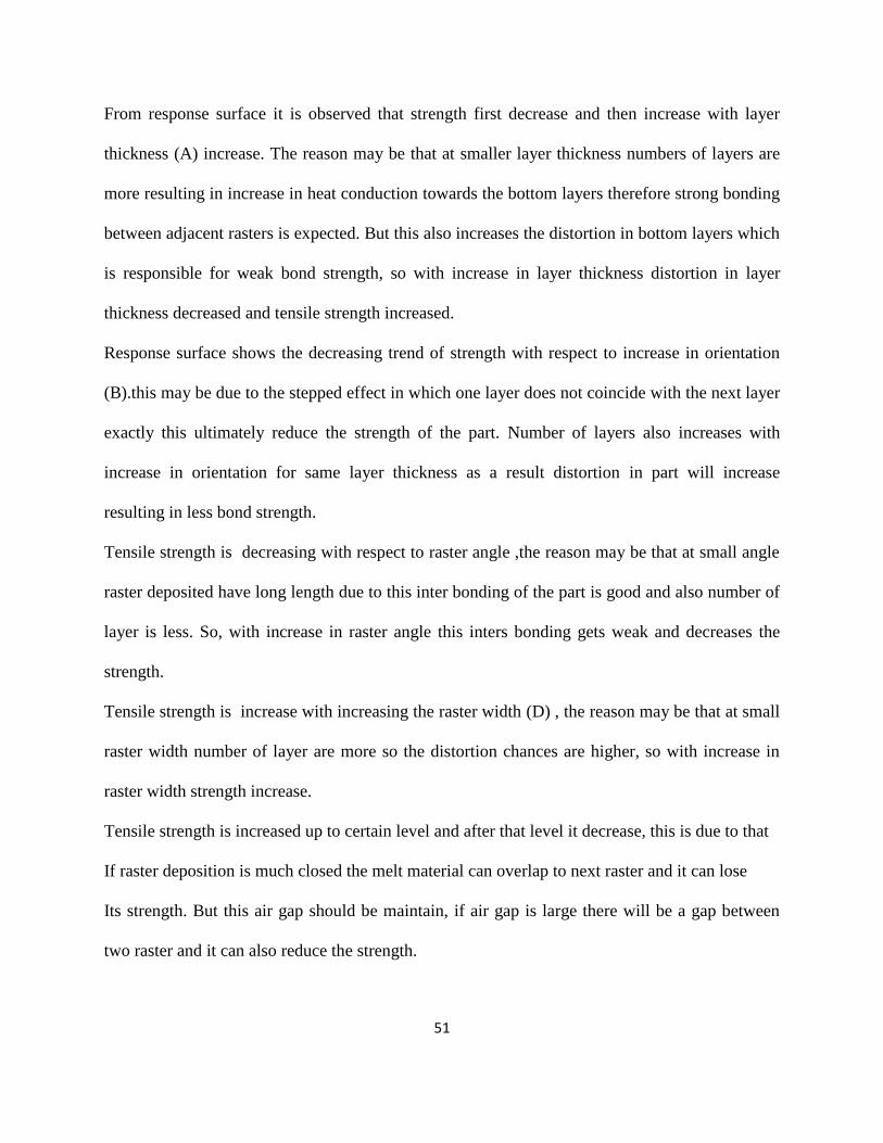
51

From response surface it is observed that strength first decrease and then increase with layer

thickness (A) increase. The reason may be that at smaller layer thickness numbers of layers are

more resulting in increase in heat conduction towards the bottom layers therefore strong bonding

between adjacent rasters is expected. But this also increases the distortion in bottom layers which

is responsible for weak bond strength, so with increase in layer thickness distortion in layer

thickness decreased and tensile strength increased.

Response surface shows the decreasing trend of strength with respect to increase in orientation

(B).this may be due to the stepped effect in which one layer does not coincide with the next layer

exactly this ultimately reduce the strength of the part. Number of layers also increases with

increase in orientation for same layer thickness as a result distortion in part will increase

resulting in less bond strength.

Tensile strength is decreasing with respect to raster angle ,the reason may be that at small angle

raster deposited have long length due to this inter bonding of the part is good and also number of

layer is less. So, with increase in raster angle this inters bonding gets weak and decreases the

strength.

Tensile strength is increase with increasing the raster width (D) , the reason may be that at small

raster width number of layer are more so the distortion chances are higher, so with increase in

raster width strength increase.

Tensile strength is increased up to certain level and after that level it decrease, this is due to that

If raster deposition is much closed the melt material can overlap to next raster and it can lose

Its strength. But this air gap should be maintain, if air gap is large there will be a gap between

two raster and it can also reduce the strength.

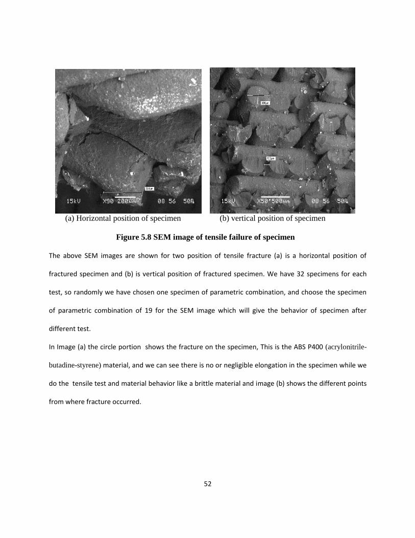
52

(a) Horizontal position of specimen (b) vertical position of specimen

Figure 5.8 SEM image of tensile failure of specimen

The above SEM images are shown for two position of tensile fracture (a) is a horizontal position of

fractured specimen and (b) is vertical position of fractured specimen. We have 32 specimens for each

test, so randomly we have chosen one specimen of parametric combination, and choose the specimen

of parametric combination of 19 for the SEM image which will give the behavior of specimen after

different test.

In Image (a) the circle portion shows the fracture on the specimen, This is the ABS P400 (acrylonitrile-

butadine-styrene) material, and we can see there is no or negligible elongation in the specimen while we

do the tensile test and material behavior like a brittle material and image (b) shows the different points

from where fracture occurred.

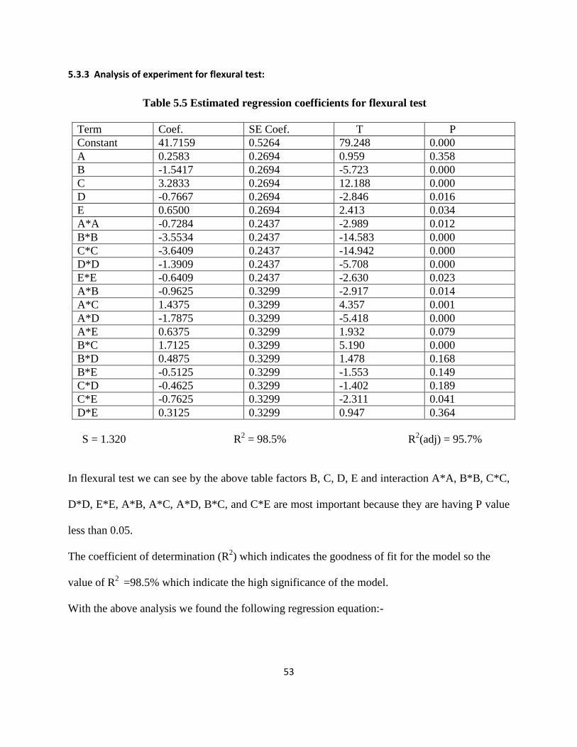
53

5.3.3 Analysis of experiment for flexural test:

Table 5.5 Estimated regression coefficients for flexural test

Term Coef. SE Coef. T P

Constant 41.7159 0.5264 79.248 0.000

A 0.2583 0.2694 0.959 0.358

B -1.5417 0.2694 -5.723 0.000

C 3.2833 0.2694 12.188 0.000

D -0.7667 0.2694 -2.846 0.016

E 0.6500 0.2694 2.413 0.034

A*A -0.7284 0.2437 -2.989 0.012

B*B -3.5534 0.2437 -14.583 0.000

C*C -3.6409 0.2437 -14.942 0.000

D*D -1.3909 0.2437 -5.708 0.000

E*E -0.6409 0.2437 -2.630 0.023

A*B -0.9625 0.3299 -2.917 0.014

A*C 1.4375 0.3299 4.357 0.001

A*D -1.7875 0.3299 -5.418 0.000

A*E 0.6375 0.3299 1.932 0.079

B*C 1.7125 0.3299 5.190 0.000

B*D 0.4875 0.3299 1.478 0.168

B*E -0.5125 0.3299 -1.553 0.149

C*D -0.4625 0.3299 -1.402 0.189

C*E -0.7625 0.3299 -2.311 0.041

D*E 0.3125 0.3299 0.947 0.364

S = 1.320 R2 = 98.5% R

2(adj) = 95.7%

In flexural test we can see by the above table factors B, C, D, E and interaction A*A, B*B, C*C,

D*D, E*E, A*B, A*C, A*D, B*C, and C*E are most important because they are having P value

less than 0.05.

The coefficient of determination (R2) which indicates the goodness of fit for the model so the

value of R2

=98.5% which indicate the high significance of the model.

With the above analysis we found the following regression equation:-

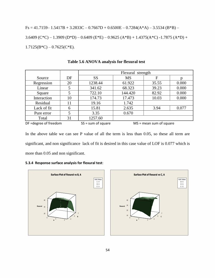
54

Fs = 41.7159– 1.5417B + 3.2833C – 0.7667D + 0.6500E – 0.7284(A*A) – 3.5534 (B*B) –

3.6409 (C*C) – 1.3909 (D*D) – 0.6409 (E*E) – 0.9625 (A*B) + 1.4375(A*C) -1.7875 (A*D) +

1.7125(B*C) – 0.7625(C*E).

Table 5.6 ANOVA analysis for flexural test

Source DF

Flexural strength

SS MS F p

Regression 20 1238.44 61.922 35.55 0.000

Linear 5 341.62 68.323 39.23 0.000

Square 5 722.10 144.420 82.92 0.000

Interaction 10 174.73 17.473 10.03 0.000

Residual 11 19.16 1.742

Lack of fit 6 15.81 2.635 3.94 0.077

Pure error 5 3.35 0.670

Total 31 1257.60

DF =degree of freedom SS = sum of square MS = mean sum of square

In the above table we can see P value of all the term is less than 0.05, so these all term are

significant, and non significance lack of fit is desired in this case value of LOF is 0.077 which is

more than 0.05 and non significant.

5.3.4 Response surface analysis for flexural test:

2

flexural

20

0

30

B

40

-20 -2

2A

Hold Values

C 0

D 0

E 0

Surface Plot of flexural vs B, A

2

flexural

10

20

0

30

C

40

-20 -2

2A

Hold Values

B 0

D 0

E 0

Surface Plot of flexural vs C, A

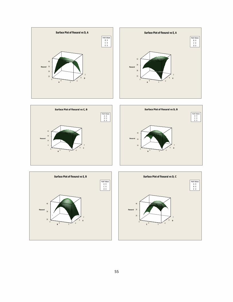
55

2

flexural

25

30

0

35

D

40

-20 -2

2A

Hold Values

B 0

C 0

E 0

Surface Plot of flexural vs D, A

2

flexural

330

36

39

E

42

-20 -2

2A

Hold Values

B 0

C 0

D 0

Surface Plot of flexural vs E, A

2

flexural

0

0

15

C

30

45

-20 -2

2B

Hold Values

A 0

D 0

E 0

Surface Plot of flexural vs C, B

2

flexural

20

0

30

D

40

-20 -2

2B

Hold Values

A 0

C 0

E 0

Surface Plot of flexural vs D, B

2

flexural

20 0

30

E

40

-20 -2

2B

Hold Values

A 0

C 0

D 0

Surface Plot of flexural vs E, B

2

flexural

20

0

30

D

40

-20 -2

2C

Hold Values

A 0

B 0

E 0

Surface Plot of flexural vs D, C

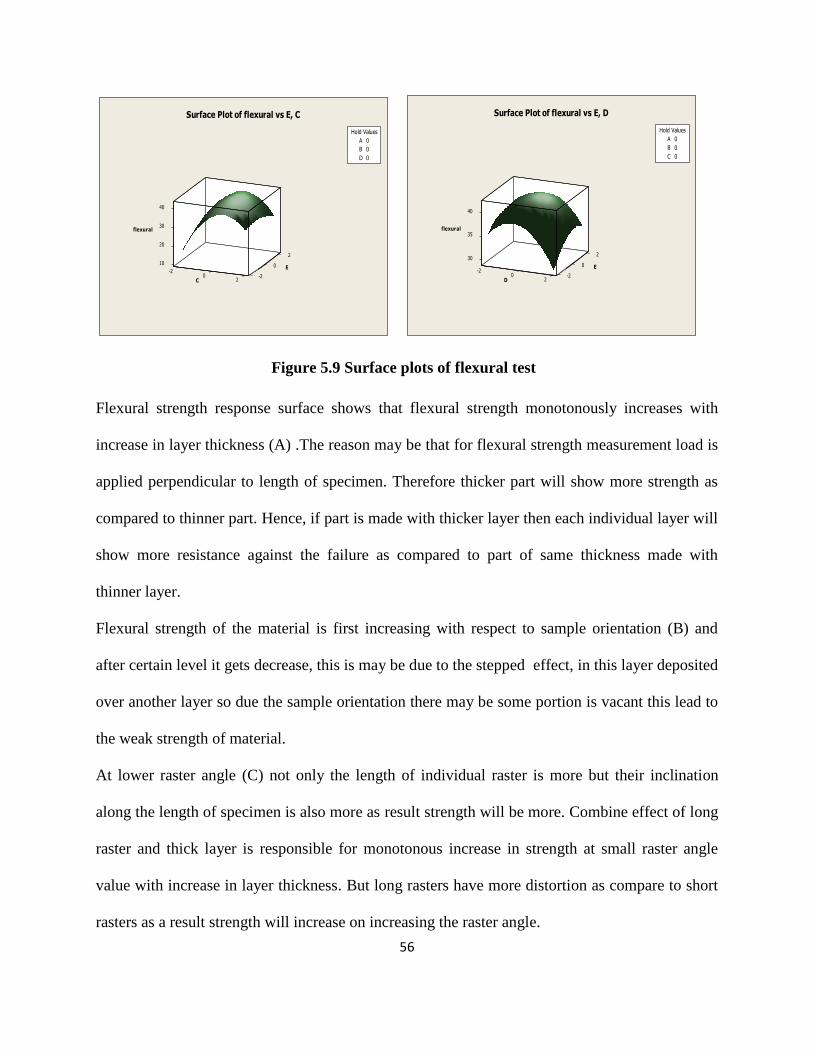
56

2

flexural

10 0

20

30

E

40

-20 -2

2C

Hold Values

A 0

B 0

D 0

Surface Plot of flexural vs E, C

2

flexural

30

0

35

E

40

-20 -2

2D

Hold Values

A 0

B 0

C 0

Surface Plot of flexural vs E, D

Figure 5.9 Surface plots of flexural test

Flexural strength response surface shows that flexural strength monotonously increases with

increase in layer thickness (A) .The reason may be that for flexural strength measurement load is

applied perpendicular to length of specimen. Therefore thicker part will show more strength as

compared to thinner part. Hence, if part is made with thicker layer then each individual layer will

show more resistance against the failure as compared to part of same thickness made with

thinner layer.

Flexural strength of the material is first increasing with respect to sample orientation (B) and

after certain level it gets decrease, this is may be due to the stepped effect, in this layer deposited

over another layer so due the sample orientation there may be some portion is vacant this lead to

the weak strength of material.

At lower raster angle (C) not only the length of individual raster is more but their inclination

along the length of specimen is also more as result strength will be more. Combine effect of long

raster and thick layer is responsible for monotonous increase in strength at small raster angle

value with increase in layer thickness. But long rasters have more distortion as compare to short

rasters as a result strength will increase on increasing the raster angle.

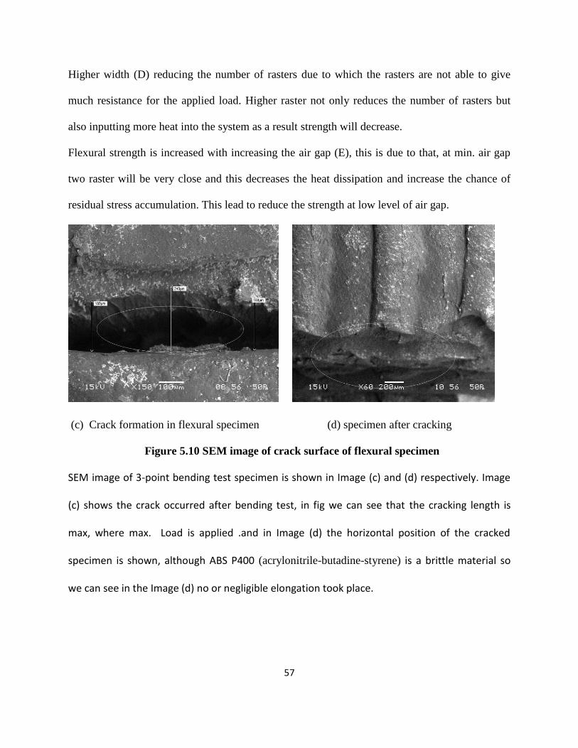
57

Higher width (D) reducing the number of rasters due to which the rasters are not able to give

much resistance for the applied load. Higher raster not only reduces the number of rasters but

also inputting more heat into the system as a result strength will decrease.

Flexural strength is increased with increasing the air gap (E), this is due to that, at min. air gap

two raster will be very close and this decreases the heat dissipation and increase the chance of

residual stress accumulation. This lead to reduce the strength at low level of air gap.

(c) Crack formation in flexural specimen (d) specimen after cracking

Figure 5.10 SEM image of crack surface of flexural specimen

SEM image of 3-point bending test specimen is shown in Image (c) and (d) respectively. Image

(c) shows the crack occurred after bending test, in fig we can see that the cracking length is

max, where max. Load is applied .and in Image (d) the horizontal position of the cracked

specimen is shown, although ABS P400 (acrylonitrile-butadine-styrene) is a brittle material so

we can see in the Image (d) no or negligible elongation took place.

58

5.3.5 Analysis of experiment for impact test:

Table 5.7 Estimated regression coefficients for impact test

Term Coef. SE Coef. T P

Constant 14.9724 0.15296 97.884 0.000

A 0.2004 0.07828 2.560 0.027

B 0.1971 0.07828 2.518 0.029

C -0.1779 0.07828 -2.273 0.044

D 0.0588 0.07828 0.751 0.469

E 0.6429 0.07828 8.213 0.000

A*A -0.7549 0.07081 -10.661 0.000

B*B -0.8224 0.07081 -11.614 0.000

C*C -0.4974 0.07081 -7.025 0.000

D*D -0.7349 0.07081 -10.379 0.000

E*E -0.4849 0.07081 -6.848 0.000

A*B 0.1444 0.09587 1.506 0.160

A*C -0.6556 0.09587 -6.838 0.000

A*D -0.0606 0.09587 -0.632 0.540

A*E 0.0506 0.09587 0.528 0.608

B*C 0.1569 0.09587 1.636 0.130

B*D -0.3481 0.09587 -3.631 0.004

B*E -0.1869 0.09587 -1.949 0.077

C*D -0.0106 0.09587 -0.111 0.914

C*E -0.1369 0.09587 -1.428 0.181

D*E -0.1044 0.09587 -1.089 0.300

S = 0.3835 R2 = 97.9% R

2 (adj) =94.0%

With the above analysis we found factors A, B, C, E and interaction A*A, B*B, C*C, D*D, E*E,

A*C, B*D.

The coefficient of determination (R2) which indicates the goodness of fit for the model so the

value of R2

=97.9% which indicate the high significance of the model.

With the above analysis we found the following regression equation:-

Is = 14.9724 + 0.2004A + 0.1971B – 0.1779C + 0.6429E – 0.7549(A*A) – 0.8224(B*B) -

0.4974 (C*C) – 0.7349 (D*D) - 0.4849 (E*E) – 0.6556 (A*C) – 0.3481(B*D) .

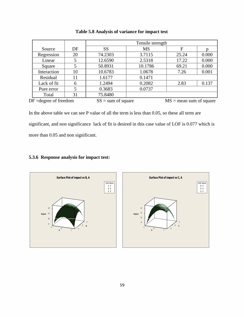
59

Table 5.8 Analysis of variance for impact test

Source DF

Tensile strength

SS MS F p

Regression 20 74.2303 3.7115 25.24 0.000

Linear 5 12.6590 2.5318 17.22 0.000

Square 5 50.8931 10.1786 69.21 0.000

Interaction 10 10.6783 1.0678 7.26 0.001

Residual 11 1.6177 0.1471

Lack of fit 6 1.2494 0.2082 2.83 0.137

Pure error 5 0.3683 0.0737

Total 31 75.8480

DF =degree of freedom SS = sum of square MS = mean sum of square

In the above table we can see P value of all the term is less than 0.05, so these all term are

significant, and non significance lack of fit is desired in this case value of LOF is 0.077 which is

more than 0.05 and non significant.

5.3.6 Response analysis for impact test:

2

impact

8

10

0

12

B

14

-20 -2

2A

Hold Values

C 0

D 0

E 0

Surface Plot of impact vs B, A

2

impact

8

0

10

12

C

14

-20 -2

2A

Hold Values

B 0

D 0

E 0

Surface Plot of impact vs C, A

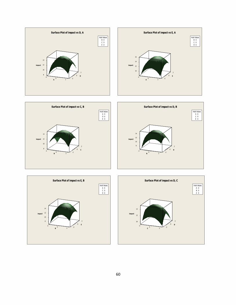
60

2

impact

8

10

0

12

D

14

-20 -2

2A

Hold Values

B 0

C 0

E 0

Surface Plot of impact vs D, A

2

impact

10

0

12

E

14

16

-20 -2

2A

Hold Values

B 0

C 0

D 0

Surface Plot of impact vs E, A

2

impact

8

10

0

12

C

14

-20 -2

2B

Hold Values

A 0

D 0

E 0

Surface Plot of impact vs C, B

2

impact

8

0

10

12

D

14

-20 -2

2B

Hold Values

A 0

C 0

E 0

Surface Plot of impact vs D, B

2

impact

8

0

10

12

E

14

-20 -2

2B

Hold Values

A 0

C 0

D 0

Surface Plot of impact vs E, B

2

impact

10

0

12

D

14

-20 -2

2C

Hold Values

A 0

B 0

E 0

Surface Plot of impact vs D, C

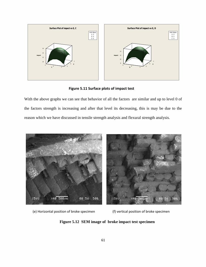
61

2

impact

10

0

12

E

14

16

-20 -2

2C

Hold Values

A 0

B 0

D 0

Surface Plot of impact vs E, C

2

impact

8

10

0

12

E

14

-20 -2

2D

Hold Values

A 0

B 0

C 0

Surface Plot of impact vs E, D

Figure 5.11 Surface plots of impact test

With the above graphs we can see that behavior of all the factors are similar and up to level 0 of

the factors strength is increasing and after that level its decreasing, this is may be due to the

reason which we have discussed in tensile strength analysis and flexural strength analysis.

(e) Horizontal position of broke specimen (f) vertical position of broke specimen

Figure 5.12 SEM image of broke impact test specimen

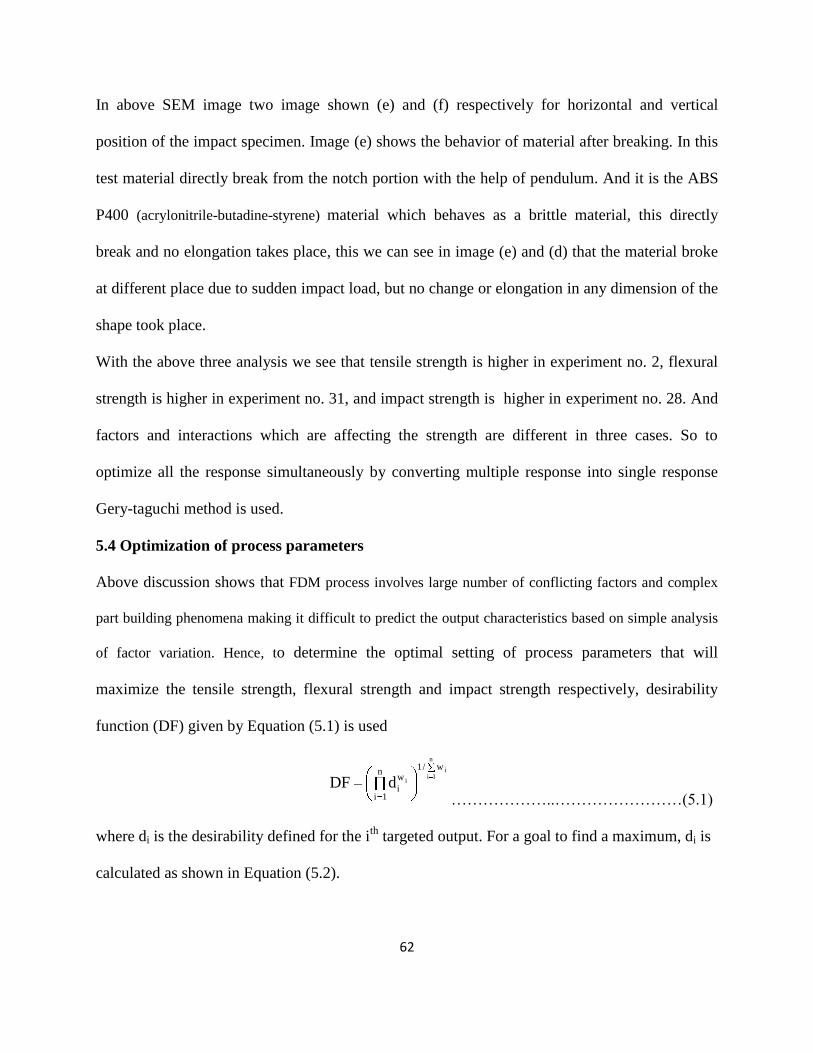
62

In above SEM image two image shown (e) and (f) respectively for horizontal and vertical

position of the impact specimen. Image (e) shows the behavior of material after breaking. In this

test material directly break from the notch portion with the help of pendulum. And it is the ABS

P400 (acrylonitrile-butadine-styrene) material which behaves as a brittle material, this directly

break and no elongation takes place, this we can see in image (e) and (d) that the material broke

at different place due to sudden impact load, but no change or elongation in any dimension of the

shape took place.

With the above three analysis we see that tensile strength is higher in experiment no. 2, flexural

strength is higher in experiment no. 31, and impact strength is higher in experiment no. 28. And

factors and interactions which are affecting the strength are different in three cases. So to

optimize all the response simultaneously by converting multiple response into single response

Gery-taguchi method is used.

5.4 Optimization of process parameters

Above discussion shows that FDM process involves large number of conflicting factors and complex

part building phenomena making it difficult to predict the output characteristics based on simple analysis

of factor variation. Hence, to determine the optimal setting of process parameters that will

maximize the tensile strength, flexural strength and impact strength respectively, desirability

function (DF) given by Equation (5.1) is used

n

1ii

i

w/1n

1i

w

idDF………………..……………………(5.1)

where di is the desirability defined for the ith

targeted output. For a goal to find a maximum, di is

calculated as shown in Equation (5.2).

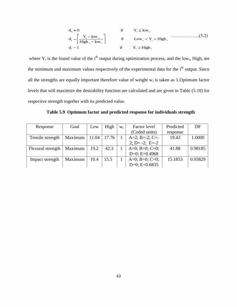
63

iii

iii

ii

iii

iii

HighYif1d

HighYLowiflowHigh

lowYd

lowYif0d

……………....(5.2)

where Yi is the found value of the ith

output during optimization process, and the lowi, Highi are

the minimum and maximum values respectively of the experimental data for the ith

output. Since

all the strengths are equally important therefore value of weight wi is taken as 1.Optimum factor

levels that will maximize the desirability function are calculated and are given in Table (5.10) for

respective strength together with its predicted value.

Table 5.9 Optimum factor and predicted response for individuals strength

Response Goal Low High wi Factor level

(Coded units)

Predicted

response

DF

Tensile strength Maximum 11.04 17.76 1 A=2; B=-2; C=-

2; D= -2; E=-2

19.43 1.0000

Flexural strength Maximum 19.2 42.3 1 A=0; B=0; C=0;

D=0; E=0.4968

41.88 0.98185

Impact strength Maximum 10.4 15.5 1 A=0; B=0; C=0;

D=0; E=0.6835

15.1853 0.93829

CHAPTER 6

______________________________________________________________________________

GREY – BASED TAGUCHI METHOD

64

6. Grey-based taguchi method

6 .1 Introduction :

Taguchi’s philosophy, developed by Dr. Genichi Taguchi, is an efficient tool for the design of

high quality manufacturing system [30]. It is a method based on Orthogonal Array experiments

which provides much-reduced variance for the experiment resulting optimal setting of process

control parameters. Orthogonal Array provides a set of well-balanced experiments with less

number of experimental runs. In order to evaluate the optimal parameter setting, Taguchi method

uses a statistical measure of performance called signal-to-noise ratio that takes both the mean and

the variability into account. The S/N ratio is the ratio of the mean (signal) to the standard

deviation (noise). The ratio depends on the quality characteristics of the product/process to be

optimized. The standard S/N ratios generally used are Nominal-is-Best (NB), lower-the-better

(LB) and Higher-the-Better (HB). The optimal setting is the parametric combination, which has

the highest S/N ratio. However, traditional Taguchi method cannot solve multi-objective

optimization problem. This can be achieved by grey based Taguchi method. In grey relational

analysis, experimental data i.e. measured features of quality characteristics of the product are

first normalized ranging from zero to one. This process is known as grey relational generation.

Next, based on normalized experimental data, grey relational coefficient is calculated to

represent the correlation between the desired and actual experimental data. Then, overall grey

relational grade is determined by averaging the grey relational coefficient corresponding to

selected responses. The overall performance characteristic of the multiple response process

depends on the calculated overall grey relational grade. This approach converts a multiple-

response process optimization problem into a single response optimization situation with the

objective function is overall grey relational grade. Using grey-Taguchi method, the optimal

parametric combination is then evaluated by maximizing the S/N ratio of the overall grey

relational grade.

65

6.2 Grey-relational analysis:

Data preprocessing:

Grey data processing must be performed before Grey correlation coefficients can be calculated.

A series of various units must be transformed to be dimensionless. Usually, each series is

normalized by dividing the data in the original series by their average. Let the original reference

sequence and sequence for comparison be represented as xo(k) and xi (k), i =1, 2, ...,m; k =1, 2,

..., n, respectively, where m is the total number of experiment to be considered, and n is the total

number of observation data. Data preprocessing converts the original sequence to a comparable

sequence [30]. Several methodologies of preprocessing data can be used in Grey relation

analysis, depending on the characteristics of the original sequence. If the target value of the

original sequence is “the-larger-the-better”, then the original sequence is normalized as follows:

If the expectancy is smaller- the –better, then the original sequence should be normalized as follow.

However, there is a definite target value to be achieved; the original sequence will be normalized

in the form.

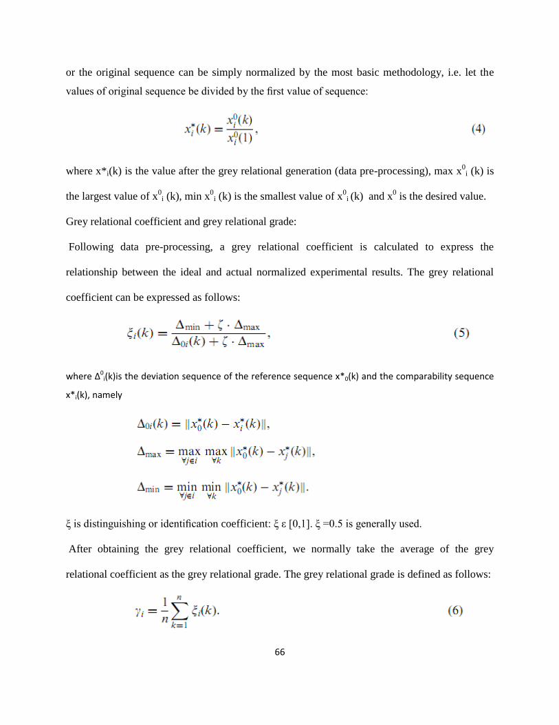
66

or the original sequence can be simply normalized by the most basic methodology, i.e. let the

values of original sequence be divided by the first value of sequence:

where x*i(k) is the value after the grey relational generation (data pre-processing), max x0i (k) is

the largest value of x0i (k), min x

0i (k) is the smallest value of x

0i (k) and x

0 is the desired value.

Grey relational coefficient and grey relational grade:

Following data pre-processing, a grey relational coefficient is calculated to express the

relationship between the ideal and actual normalized experimental results. The grey relational

coefficient can be expressed as follows:

where Δ0i(k)is the deviation sequence of the reference sequence x*0(k) and the comparability sequence

x*i(k), namely

ξ is distinguishing or identification coefficient: ξ ε [0,1]. ξ =0.5 is generally used.

After obtaining the grey relational coefficient, we normally take the average of the grey

relational coefficient as the grey relational grade. The grey relational grade is defined as follows:

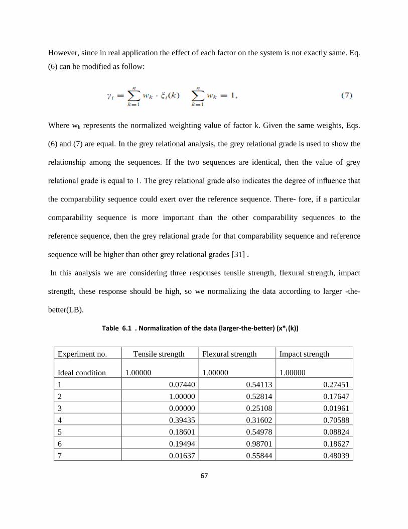
67

However, since in real application the effect of each factor on the system is not exactly same. Eq.

(6) can be modified as follow:

Where wk represents the normalized weighting value of factor k. Given the same weights, Eqs.

(6) and (7) are equal. In the grey relational analysis, the grey relational grade is used to show the

relationship among the sequences. If the two sequences are identical, then the value of grey

relational grade is equal to 1. The grey relational grade also indicates the degree of influence that

the comparability sequence could exert over the reference sequence. There- fore, if a particular

comparability sequence is more important than the other comparability sequences to the

reference sequence, then the grey relational grade for that comparability sequence and reference

sequence will be higher than other grey relational grades [31] .

In this analysis we are considering three responses tensile strength, flexural strength, impact

strength, these response should be high, so we normalizing the data according to larger -the-

better(LB).

Table 6.1 . Normalization of the data (larger-the-better) (x*I (k))

Experiment no. Tensile strength Flexural strength Impact strength

Ideal condition

1.00000

1.00000

1.00000

1 0.07440 0.54113 0.27451

2 1.00000 0.52814 0.17647

3 0.00000 0.25108 0.01961

4 0.39435 0.31602 0.70588

5 0.18601 0.54978 0.08824

6 0.19494 0.98701 0.18627

7 0.01637 0.55844 0.48039

68

Table 6.2 The deviation sequence (Δo,i(k))

Experiment no.

Tensile strength,

Δo,i(1)

Flexural strength,

Δo,i(2)

Impact strength,

Δo,i(3)

1 0.92560 0.45887 0.72549

2 0.00000 0.47186 0.82353

3 1.00000 0.74892 0.98039

4 0.60565 0.68398 0.29412

5 0.81399 0.45022 0.91176

6 0.80506 0.01299 0.81373

8 0.18601 0.84848 0.23529

9 0.84673 0.47186 0.07647

10 0.76339 0.53680 0.66667

11 0.00000 0.45455 0.09804

12 0.12202 0.00000 0.29412

13 0.28274 0.54545 0.47059

14 0.67857 0.54978 0.00000

15 0.00149 0.71429 0.25490

16 0.78423 0.64069 0.19020

17 0.01488 0.88745 0.21569

18 0.75298 0.86147 0.34118

19 0.81994 0.55411 0.07843

20 0.00000 0.21645 0.37255

21 0.67857 0.09091 0.58824

22 0.18750 0.64935 0.37255

23 0.18155 0.79221 0.19608

24 0.79762 0.72727 0.39216

25 0.43750 0.88745 0.21569

26 0.20238 0.89177 0.76471

27 0.61905 0.99567 0.88235

28 0.78274 0.90476 1.00000

29 0.72321 0.96970 0.84314

30 0.79762 0.94805 0.90196

31 0.66369 1.00000 0.92157

32 0.72321 0.97835 0.88235

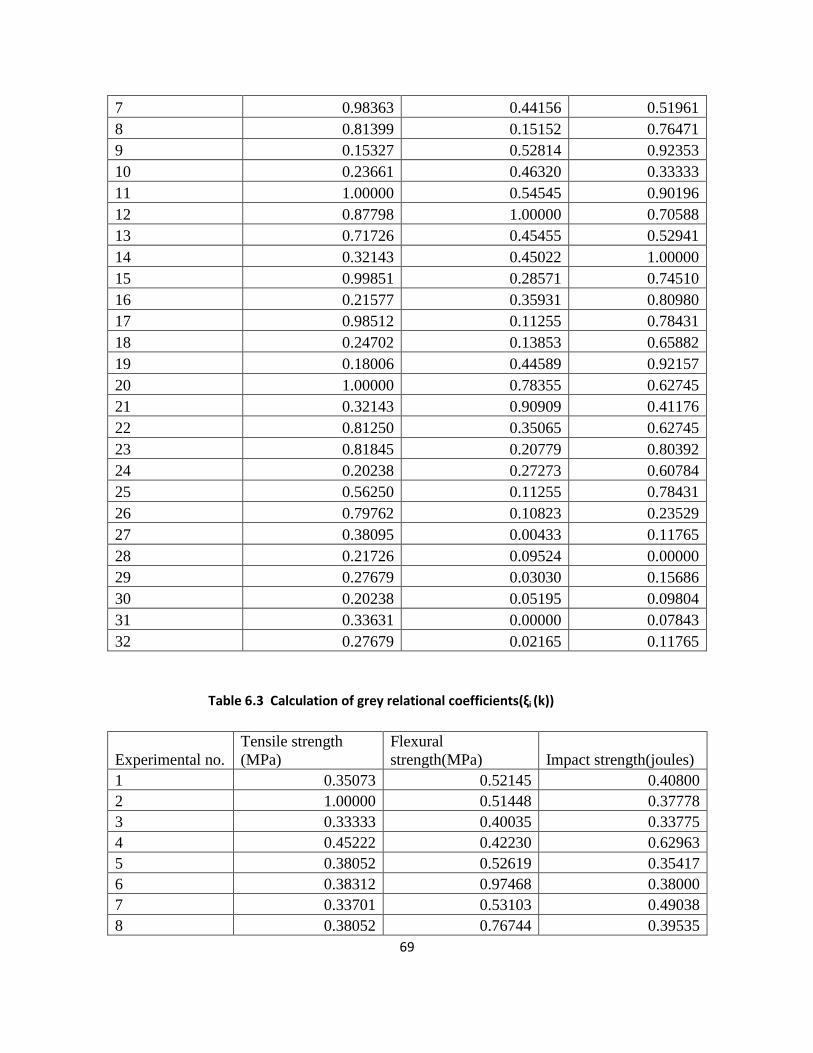
69

7 0.98363 0.44156 0.51961

8 0.81399 0.15152 0.76471

9 0.15327 0.52814 0.92353

10 0.23661 0.46320 0.33333

11 1.00000 0.54545 0.90196

12 0.87798 1.00000 0.70588

13 0.71726 0.45455 0.52941

14 0.32143 0.45022 1.00000

15 0.99851 0.28571 0.74510

16 0.21577 0.35931 0.80980

17 0.98512 0.11255 0.78431

18 0.24702 0.13853 0.65882

19 0.18006 0.44589 0.92157

20 1.00000 0.78355 0.62745

21 0.32143 0.90909 0.41176

22 0.81250 0.35065 0.62745

23 0.81845 0.20779 0.80392

24 0.20238 0.27273 0.60784

25 0.56250 0.11255 0.78431

26 0.79762 0.10823 0.23529

27 0.38095 0.00433 0.11765

28 0.21726 0.09524 0.00000

29 0.27679 0.03030 0.15686

30 0.20238 0.05195 0.09804

31 0.33631 0.00000 0.07843

32 0.27679 0.02165 0.11765

Table 6.3 Calculation of grey relational coefficients(ξi (k))

Experimental no.

Tensile strength

(MPa)

Flexural

strength(MPa) Impact strength(joules)

1 0.35073 0.52145 0.40800

2 1.00000 0.51448 0.37778

3 0.33333 0.40035 0.33775

4 0.45222 0.42230 0.62963

5 0.38052 0.52619 0.35417

6 0.38312 0.97468 0.38000

7 0.33701 0.53103 0.49038

8 0.38052 0.76744 0.39535

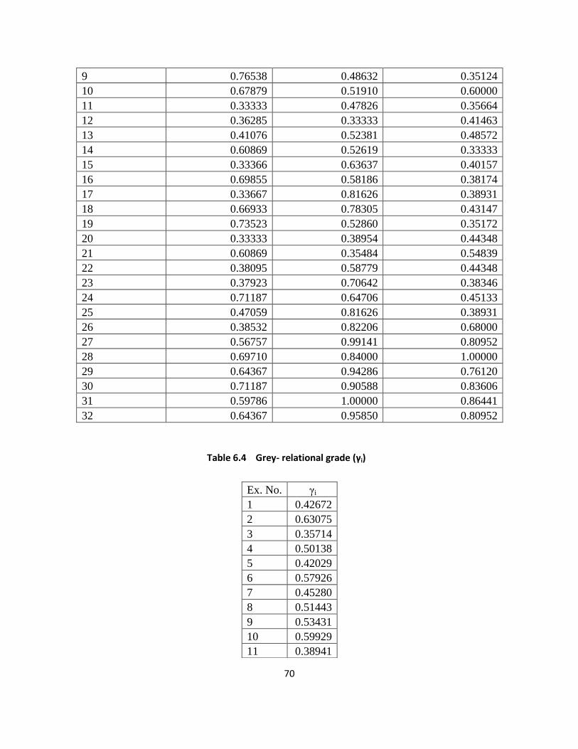
70

9 0.76538 0.48632 0.35124

10 0.67879 0.51910 0.60000

11 0.33333 0.47826 0.35664

12 0.36285 0.33333 0.41463

13 0.41076 0.52381 0.48572

14 0.60869 0.52619 0.33333

15 0.33366 0.63637 0.40157

16 0.69855 0.58186 0.38174

17 0.33667 0.81626 0.38931

18 0.66933 0.78305 0.43147

19 0.73523 0.52860 0.35172

20 0.33333 0.38954 0.44348

21 0.60869 0.35484 0.54839

22 0.38095 0.58779 0.44348

23 0.37923 0.70642 0.38346

24 0.71187 0.64706 0.45133

25 0.47059 0.81626 0.38931

26 0.38532 0.82206 0.68000

27 0.56757 0.99141 0.80952

28 0.69710 0.84000 1.00000

29 0.64367 0.94286 0.76120

30 0.71187 0.90588 0.83606

31 0.59786 1.00000 0.86441

32 0.64367 0.95850 0.80952

Table 6.4 Grey- relational grade (γi)

Ex. No. γi

1 0.42672

2 0.63075

3 0.35714

4 0.50138

5 0.42029

6 0.57926

7 0.45280

8 0.51443

9 0.53431

10 0.59929

11 0.38941

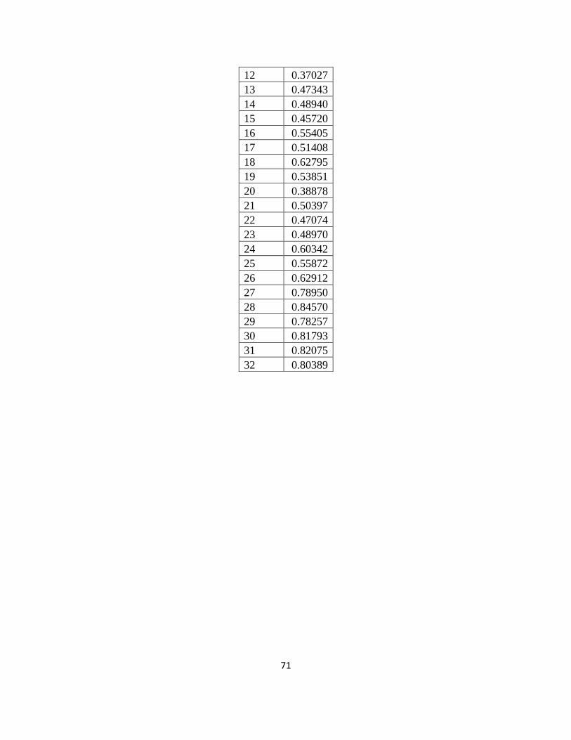
71

12 0.37027

13 0.47343

14 0.48940

15 0.45720

16 0.55405

17 0.51408

18 0.62795

19 0.53851

20 0.38878

21 0.50397

22 0.47074

23 0.48970

24 0.60342

25 0.55872

26 0.62912

27 0.78950

28 0.84570

29 0.78257

30 0.81793

31 0.82075

32 0.80389

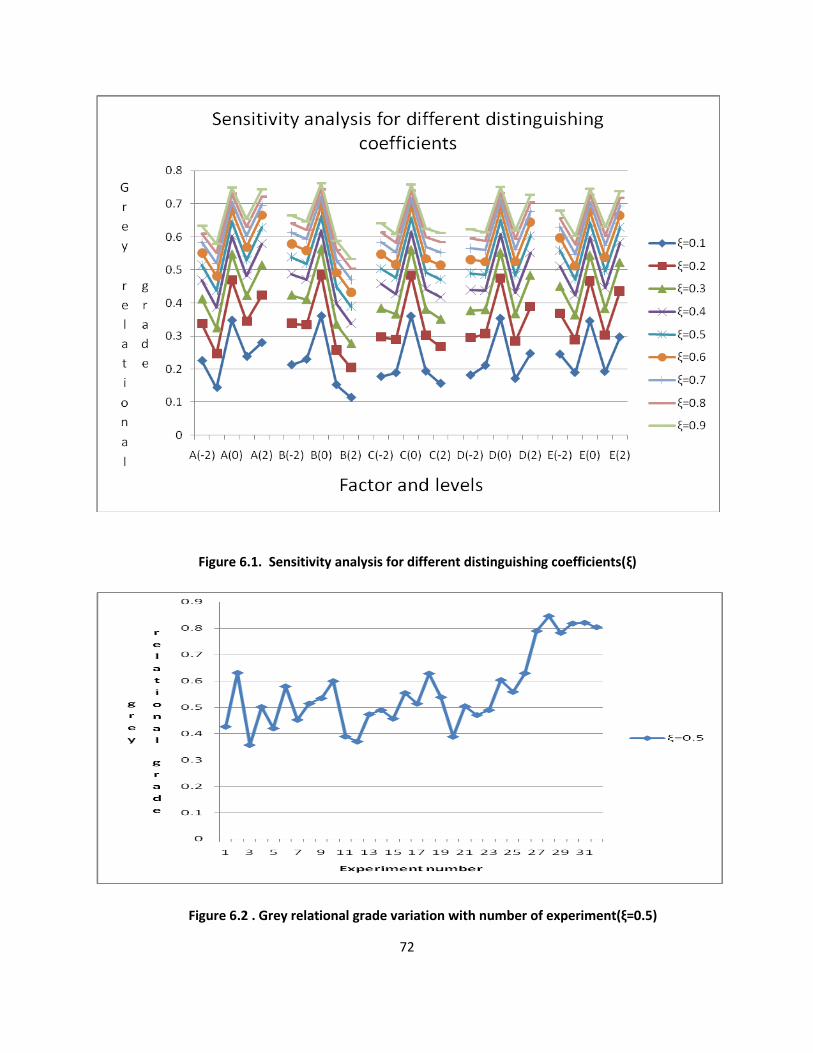
72

Figure 6.1. Sensitivity analysis for different distinguishing coefficients(ξ)

Figure 6.2 . Grey relational grade variation with number of experiment(ξ=0.5)

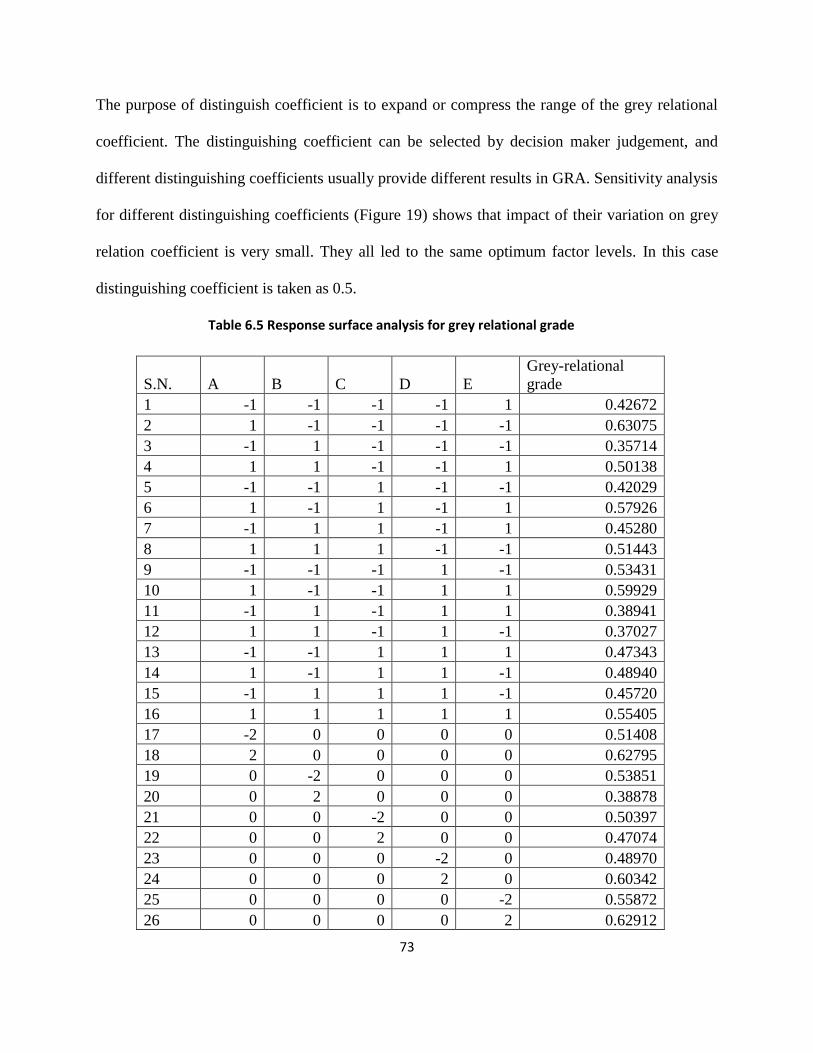
73

The purpose of distinguish coefficient is to expand or compress the range of the grey relational

coefficient. The distinguishing coefficient can be selected by decision maker judgement, and

different distinguishing coefficients usually provide different results in GRA. Sensitivity analysis

for different distinguishing coefficients (Figure 19) shows that impact of their variation on grey

relation coefficient is very small. They all led to the same optimum factor levels. In this case

distinguishing coefficient is taken as 0.5.

Table 6.5 Response surface analysis for grey relational grade

S.N. A B C D E

Grey-relational

grade

1 -1 -1 -1 -1 1 0.42672

2 1 -1 -1 -1 -1 0.63075

3 -1 1 -1 -1 -1 0.35714

4 1 1 -1 -1 1 0.50138

5 -1 -1 1 -1 -1 0.42029

6 1 -1 1 -1 1 0.57926

7 -1 1 1 -1 1 0.45280

8 1 1 1 -1 -1 0.51443

9 -1 -1 -1 1 -1 0.53431

10 1 -1 -1 1 1 0.59929

11 -1 1 -1 1 1 0.38941

12 1 1 -1 1 -1 0.37027

13 -1 -1 1 1 1 0.47343

14 1 -1 1 1 -1 0.48940

15 -1 1 1 1 -1 0.45720

16 1 1 1 1 1 0.55405

17 -2 0 0 0 0 0.51408

18 2 0 0 0 0 0.62795

19 0 -2 0 0 0 0.53851

20 0 2 0 0 0 0.38878

21 0 0 -2 0 0 0.50397

22 0 0 2 0 0 0.47074

23 0 0 0 -2 0 0.48970

24 0 0 0 2 0 0.60342

25 0 0 0 0 -2 0.55872

26 0 0 0 0 2 0.62912

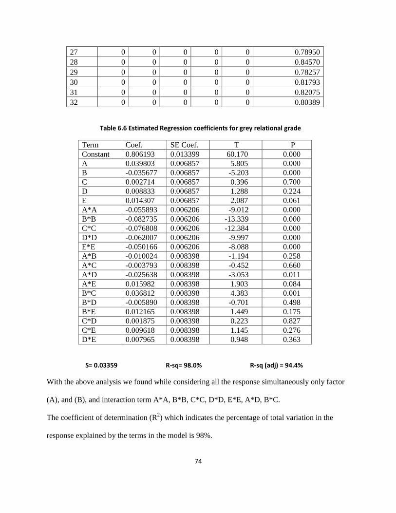
74

27 0 0 0 0 0 0.78950

28 0 0 0 0 0 0.84570

29 0 0 0 0 0 0.78257

30 0 0 0 0 0 0.81793

31 0 0 0 0 0 0.82075

32 0 0 0 0 0 0.80389

Table 6.6 Estimated Regression coefficients for grey relational grade

Term Coef. SE Coef. T P

Constant 0.806193 0.013399 60.170 0.000

A 0.039803 0.006857 5.805 0.000

B -0.035677 0.006857 -5.203 0.000

C 0.002714 0.006857 0.396 0.700

D 0.008833 0.006857 1.288 0.224

E 0.014307 0.006857 2.087 0.061

A*A -0.055893 0.006206 -9.012 0.000

B*B -0.082735 0.006206 -13.339 0.000

C*C -0.076808 0.006206 -12.384 0.000

D*D -0.062007 0.006206 -9.997 0.000

E*E -0.050166 0.006206 -8.088 0.000

A*B -0.010024 0.008398 -1.194 0.258

A*C -0.003793 0.008398 -0.452 0.660

A*D -0.025638 0.008398 -3.053 0.011

A*E 0.015982 0.008398 1.903 0.084

B*C 0.036812 0.008398 4.383 0.001

B*D -0.005890 0.008398 -0.701 0.498

B*E 0.012165 0.008398 1.449 0.175

C*D 0.001875 0.008398 0.223 0.827

C*E 0.009618 0.008398 1.145 0.276

D*E 0.007965 0.008398 0.948 0.363

S= 0.03359 R-sq= 98.0% R-sq (adj) = 94.4%

With the above analysis we found while considering all the response simultaneously only factor

(A), and (B), and interaction term A*A, B*B, C*C, D*D, E*E, A*D, B*C.

The coefficient of determination (R2) which indicates the percentage of total variation in the

response explained by the terms in the model is 98%.

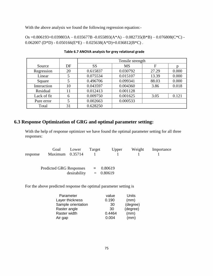
75

With the above analysis we found the following regression equation:-

Os =0.806193+0.039803A – 0.035677B -0.055893(A*A) – 0.082735(B*B) – 0.076808(C*C) -

0.062007 (D*D) - 0.050166(E*E) – 0.025638(A*D)+0.036812(B*C) .

Table 6.7 ANOVA analysis for grey relational grade

Source DF

Tensile strength

SS MS F p

Regression 20 0.615837 0.030792 27.29 0.000

Linear 5 0.075534 0.015107 13.39 0.000

Square 5 0.496706 0.099341 88.03 0.000

Interaction 10 0.043597 0.004360 3.86 0.018

Residual 11 0.012413 0.001128

Lack of fit 6 0.009750 0.001625 3.05 0.121

Pure error 5 0.002663 0.000533

Total 31 0.628250

6.3 Response Optimization of GRG and optimal parameter setting:

With the help of response optimizer we have found the optimal parameter setting for all three

responses:

Goal Lower Target Upper Weight Importance

response Maximum 0.35714 1 1 1 1

Predicted GRG Responses = 0.80619

desirability = 0.80619

For the above predicted response the optimal parameter setting is

Parameter value Units Layer thickness 0.190 (mm) Sample orientation 30 (degree) Raster angle 30 (degree) Raster width 0.4464 (mm) Air gap 0.004 (mm)

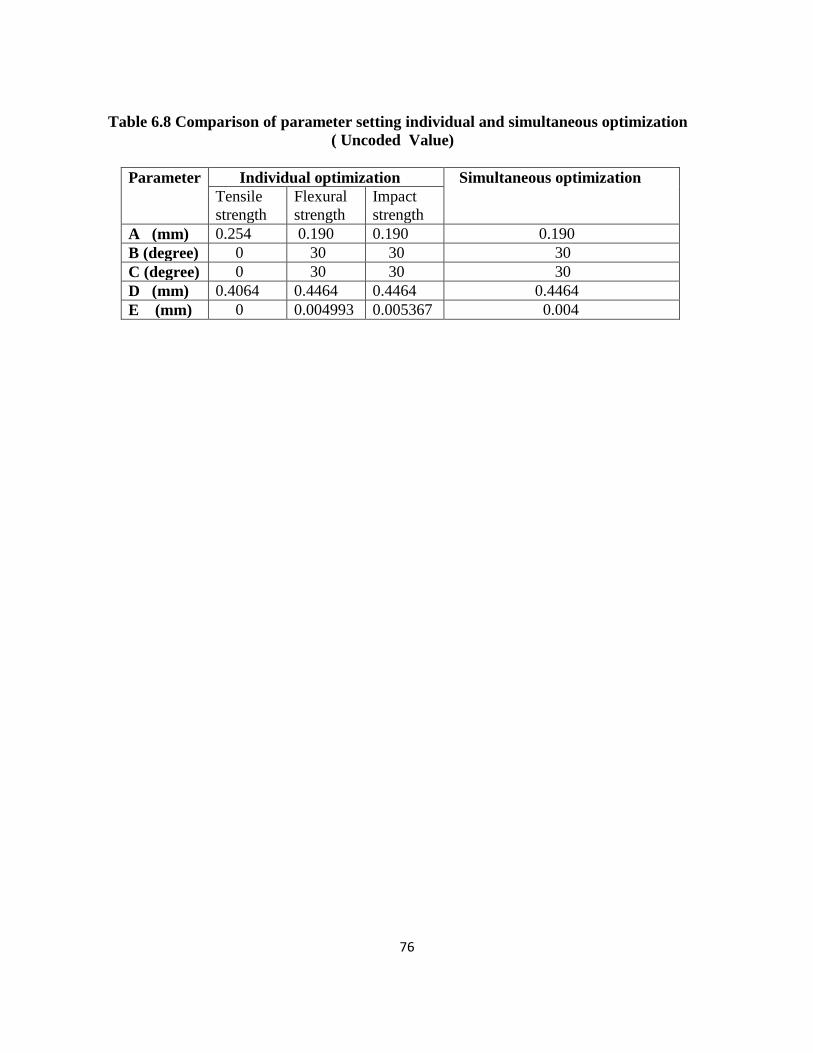
76

Table 6.8 Comparison of parameter setting individual and simultaneous optimization

( Uncoded Value)

Parameter Individual optimization Simultaneous optimization

Tensile

strength

Flexural

strength

Impact

strength

A (mm) 0.254 0.190 0.190 0.190

B (degree) 0 30 30 30

C (degree) 0 30 30 30

D (mm) 0.4064 0.4464 0.4464 0.4464

E (mm) 0 0.004993 0.005367 0.004

CHAPTER 7

______________________________________________________________________________

RESULT, CONCLUSION AND FUTURE SCOPE

77

7. Results, conclusions and future scope

7.1 Results and discussions:

The tensile strength data of ABS sample with different level of process parameter are shown in

table (2). The ultimate strength were the highest (17.76 MPa) for the layer thickness 0.222 mm,

sample orientation 15o

, raster angle 15o

, raster width 0.4264 mm, and air gap 0.002 mm

combination set and the lower strength (11.04 MPa) for layer thickness 0.158 mm, sample

orientation 45o, raster angle 15

o , raster width 0.4264 mm, and air gap 0.002 mm, the lower

strength in the solid model could have been caused by residual stress from the volumetric

shrinkage , weak interlayer bonding, or interlayer porosity. Examination of the fracture surfaces

revealed fracture paths that were controlled by either weak interlayer bonding or interlayer

porosity. Weak interlayer bonding probably was a result of residual stresses caused by

volumetric shrinkage of the polymer layers during solidification from the melt. Weak interlayer

bonding could also be caused by the low molecular diffusion and low cross-linking between the

polymer layers during deposition from the melt. In addition, the interlayer porosity reduced the

load-bearing area across the layers and hence provided an easy fracture path. The percent

elongation of the tensile specimens was <2%, and the ABS material failed in a semi-brittle

manner. Because the ABS elongation was so low.

The 3-point bending test data of ABS sample shown in table (2).the flexural strength are greater

than the tensile strengths because the modulus of rupture measure the maximum strength at the

outer fiber of the beam. This is expected because during bending, the sample is subjected to both

compressive and tensile load in this test flexural strength is highest (42.3 MPa) for the layer

thickness 0.190 mm, sample orientation 30o

, raster angle 30o, raster width 0.4464 mm, and air

gap were 0.004 mm. and min. flexural strength (19.20 MPa) for layer thickness 0.222 mm,

78

sample orientation 45o, raster angle 15

o , raster width 0.4664 mm, and air gap 0.002 mm. again as

in the tensile testing, this low flexural strength is due to rapid prototyping sample having weak

interlayer bonding or interlayer porosity.

During impact testing, the material is subjected to quick, intense blow by a hammer pendulum.

The impact test measures the energy absorption or the toughness of the material. The V-notched

specimen evaluates the materials resistance to crack propagation. In this test we found ultimate

impact strength (15.50 joule) for the parametric combination of layer thickness 0.190 mm,

sample orientation 30o, raster angle at 30

o, raster width 0.4464 mm, and air gap 0.004 mm. and

min. impact strength (10.4 joule) for the parametric combination of layer thickness 0.222 mm,

sample orientation 15o, raster angle 45

o, raster width 0.4664 mm, and air gap 0.002 mm. in FDM,

heating and rapid cooling cycles of the material result in non-uniform temperature gradients.

This cause stresses to build up leading to distortion, dimensional inaccuracy and inner layer

cracking or de-lamination. The reasons attributed to non uniform heating and cooling cycles are

explained as follows:

(1) In FDM, heat is dissipated by conduction and forced convection and the reduction in

temperature caused by these processes forces the material to quickly solidify onto the

surrounding filaments. Bonding between the filaments is caused by local re-melting of

previously solidified material and diffusion. This results in uneven heating and cooling of

material and develops non uniform temperature gradients. As a result, uniform stress will not be

developed in the deposited material and it may not regain its original dimension completely.

(2) Speed at which nozzle is depositing the material may alter the heating and cooling cycle and

results in different degree of thermal gradient and thus also affects the part accuracy.

79

At lower slice thickness, nozzle deposition speed is slower as compared to higher slice

thickness. Also during deposition, nozzle stops depositing material in random manner (in

between depositing a layer and after completely depositing a layer) and return to service location

for tip cleaning. While depositing the material at the turns near the boundary of part, nozzle

speed has to be decreased and then increase to uniform speed . If deposition path length is small,

this will result in non uniform stress to build up especially near the part boundary.

(3) The pattern used to deposit a material in a layer has a significant effect on the resulting

stresses and deformation. Higher stresses will be found along the long axis of deposition line.

Therefore, short raster length is preferred along the long axis of part to reduce the stresses.

(4) Stress accumulation also increase with layer thickness and road width. But the thick layer

also means fewer layers, which may reduce the number of heating and cooling cycles. Also, a

smaller road width will input less heat into the system within the specified period of time but

requires more loops to fill a certain area. More loops means more time required for deposition of

single layer and more non uniform nozzle speed. This will keep the deposited material above its

desired temperature for regaining its original shape and in the mean time new material will be

deposited and contraction of previously deposited material will be constrained

Hence, with the response surface analysis we have seen that tensile strength, flexural strength,

and impact strength, are higher at different parametric combination, optimization of all three

responses is impossible. So grey Taguchi method is used to convert these multiple response into

a single response, and with the help of response optimizer we found out the optimal parameter

setting to maximize all three responses.

80

7.2 Conclusion:

Effect of five process parameters layer thickness, sample orientation, raster angle, raster width

and air gap are studied on three responses viz., tensile strength, flexural strength and impact

strength of test specimen. Experiments were conducted using centre composite design (CCD).

Empirical relations between each response and process parameters were determined and their

validity is proved using analysis of variance (ANOVA) and the normal probability plot of

residues. Response surface plots of respective strength shows that parameter effect are dependent

on each other and their optimal setting depends upon the level selected for other parameters. The

main reason attributed for weak strength is the distortion within the layer or between the layers.

To get the optimal level concept of simultaneous optimization of three responses desirability

function is used for maximizing the all the responses and found out the optimal parameter

setting.

7.3 Future scope:

The response surface methodology is a robust process for optimization of the single response

as well as multiple responses. In present work, optimization of three FDM responses is

considered are tensile, flexural, and impact strength. Due to time constraints, we optimized only

three responses, although compression test, fatigue test, wear test, hardness test, may be carried

out in future. Response surface methodology can be used as an analysis tool in any process when

parameters affecting the responses are identified through experimental and theoretical validation.

BIBLIOGRAPHY

81

Bibliography

1. Wiedemann, B. Jantzen (1999). Strategies and applications for rapid product and process

development in Daimler-Benz AG, Computers in industries, 39(1):11–25

2. Upcraft Steve and Fletcher Richard (2003). The Rapid prototyping technologies, Rapid

prototyping journal,23(4):318-330

3. Mansour S. and Hauge R (2003). Impact of rapid manufacturing on design for manufacturing

on design for manufacture for injection moulding, Proceedings of the institution of

mechanical enginers, Part B, Journal of engineering manufacture, 217(4): 453-461

4. Ahn Sung Hoon, Montero Michael, Odell Dan, Roundy Shad, Wright Paul K. (2002).

Anisotropic material properties of fused deposition modelling ABS, Rapid prototyping

journal, 8 (4): 248-257

5. Es. Said Os, Foyos J, Noorani R, Mandelson M, Marloth R, Pregger BA (2000). Effect of

layer orientation on mechanical properties of rapid prototyped samples, Materials and

manufacturing process,15 (1):107-122.

6. Lee C.S., Kim S.G., Kim H.J., Ahn S.H (2007), Measurement of anisotropic compressive

strength of rapid prototyping parts, Journal of materials processing technology, 187-188:

637-630.

7. Khan Z.A., Lee B.H., Abdullah J(2005) Optimization of rapid prototyping parameters for

production of flexible ABS object, Journal of materials processing technology 169 :54–61

8. Wang Tian Ming, Xi Jun Tong, Jin Ye (2007), A model research for prototype warp

deformation in the FDM process, International journal of advance manufacturing

technology, 33(11-12):1087-1096

82

9. Bellehumeur C.T., Gu P., Sun Q., Rizvi G.M. (2008). Effect of processing conditions on

the bonding quality of FDM polymer filaments, Rapid prototyping journal, 14 (2): 72-80

10. Chou K, Y Zhang (2008), A parametric study of part distortion in fused deposition

modeling using three dimensional element analysis, Proc. IMechE: Journal of engineering

manufacture, 222(B):959-967.

11. R.Anitha, S.Arunachalam, P.Radhakrishnan(2001).Critical parameter influencing the

quality of prototypes in fused deposition modelling, Journal of material processing

technology, 118, 385-388.

12. Sanat Agrawal;S.G.Dhande(2007).Analysis of mechanical error in fused deposition

process using a stochastic approach, International journal of production research.Vol.45,

No.17,1 September 2007, 3991-4012.

13. P.M.Pandey, K.thrimurthulu,N.Venkata Reddy(2004). Optimal part deposition orientation

in FDM by using a multicriteria genetic algorithm, International journal of production

research.Vol. 42, No. 19, 4069-4089.

14. Stephen W.Tsai and Edward M. Wu.A (1970). General theory of strength for anisotropic

materials, A journal of composire materials.

15. Stratasys (2004),FDM Vantage user guide version 1.1, www.stratasys.com.

16. Kathleen M. Carley, Natalia Y. Kamneva, Jeff Reminga (2004). Response surface

methodology, CASOS Technical report.

17. Jae-Seob Kwak (2005). Application of taguchi and response surface methodologies for

geometric error in surface grinding process, International journal of machine tools and

manufacturing 45(2005) 327-334.

83

18. Pilipović Ana , Raos Pero and Šercer Mladen (2009), Experimental analysis of

properties of materials for rapid prototyping, International journal of advanced

manufacturing technology, 40: 105-115

19. Levy Gideon N., Schindel Ralf, Kruth J.P., Leuven K.U. (2003). Rapid manufacturing

and rapid tooling with layer manufacturing(LM) technologies-State of the art and future

perspectives, CIRP annals-Manufacturing technology, 52(2): 589-609

20. Chockalingama K., Jawahara N., Chandrasekarb U., Ramanathana K.N. (2008).

Establishment of process model for part strength in stereolithography, Journal of

materials processing technology, DOI 10.1016/j.jmatprotec.2007.12.144

21. Hopkinson N., Hagur R.J.M., Dickens P.H. (2006). Rapid manufacturing: An industrial

revolution for the digital age, John Wiley & Sons, Ltd., England

22. Zhou M.Y., Xi J.T., Yan J.Q. (2004). Modeling and processing of functionally graded

materials for rapid prototyping, Journal of materials processing technology, 146: 396-402

23. Bernarand Alain and Fischer A (2002). New trends in rapid product development, CIRP

annals-Manufacturing technology, 51(2): 635-652

24. Pandey Pulak M., Jain Prashant K., Rao P. V. M.(2008), “Effect of delay time on part

strength in selective laser Sintering”, International journal of advance manufacturing

technology, DOI 10.1007/s00170-008-1682-3

25. Vasudevarao Bharath, Natarajan Dharma Prakash, Razdan Anshuman, Mark

Henderson(2000).Sensitivity of RP surface finish to process parameter variation, Solid

free form fabrication proceedings, The University of Texas, Austin: 252-258

26. Sameh S. Habib (2009). Study of the parameters in electric discharge machining through

response surface methodology approach, Journal of applied mathematical modelling.

84

27. Montgomery Douglas C. Design and analysis of experiments, 5th

edition, John Wiley &

sons (ASIA) Pte Ltd., Singapore

28. Noorani Rafiq (2006). Rapid prototyping: Principles and application, John Wiley & Sons,

Inc. U.S.A.

29. Ken Jones, Mark Johnson, J.J. Liou (2006). The comparison of response surface and

taguchi methods for multiple response optimization using simulation.

30. Che Chung wang, Ta-Wei Lin, Shr-Shiung Hu (2007) . Optimization of rapid prototyping

process by integrating Taguchi method with grey relational analysis, Journal of rapid

prototyping.Volume 13.Page 304-314.

31. Y. Ravi Kumar, C.S.P. Rao, T.A. Janardhan Reddy (2008). Robust process optimisation

for fused deposition modelling, International journal of manufacturing technology and

management 2008 - Vol. 14, No.1/2 pp. 228 - 245