University of South FloridaScholar Commons

Graduate Theses and Dissertations Graduate School

2008

Parametric, non-parametric and statistical modelingof stony coral reef dataArmando HoareUniversity of South Florida

Follow this and additional works at: http://scholarcommons.usf.edu/etd

Part of the American Studies Commons

This Dissertation is brought to you for free and open access by the Graduate School at Scholar Commons. It has been accepted for inclusion inGraduate Theses and Dissertations by an authorized administrator of Scholar Commons. For more information, please contactscholarcommons@usf.edu.

Scholar Commons CitationHoare, Armando, "Parametric, non-parametric and statistical modeling of stony coral reef data" (2008). Graduate Theses andDissertations.http://scholarcommons.usf.edu/etd/296

Parametric, Non-Parametric And Statistical Modeling Of Stony Coral Reef Data

by

Armando Hoare

A dissertation submitted in partial fulfillment of the requirements for the degree of

Doctor of Philosophy Department of Mathematics and Statistics

College of Arts and Sciences University of South Florida

Major Professor: Chris P. Tsokos, Ph.D. Marcus McWaters, Ph.D.

Kandethody Ramachandran, Ph.D. Gangaram S. Ladde, Ph.D.

Pamela Hallock Muller, Ph.D.

Date of Approval: April 8, 2008

Keywords: regression model, stony coral, Shannon-Wiener diversity index, Simpson's diversity index, jackknifing, bootstrap, three-parameter lognormal distribution, kernel

density estimate

© Copyright 2008 , Armando Hoare

Dedication

This dissertation is dedicated to my wife, Ana, who has walked this long path by

my side offering her love, encouragement and even professional advice all along the way.

She, above all others, has understood the demands and the sacrifices required of a

scholar. Ana has pushed me to the greater challenge of realizing my full potential. I also

dedicate this work to my beloved son, Armando. You are the reason for it all; your love,

patience and alarming wisdom have been my greatest inspiration.

It goes without saying that my brothers and sisters and their spouses have been a

godsend through it all. They have encouraged me, inspired me, loved me and have done

everything humanly possible to raise me up throughout my pursuit of an academic career.

Martha, my second mother, words can never express the extreme gratitude and respect I

have for you. Ismael and Olda, you understood what trials and challenges must be

overcome and the sacrifices that must be made to succeed at this level. Thank you,

Eduardo, for in your special way, you have helped me keep it together. Mom and Dad,

the values of perseverance and strength of mind and character that you passed on to me

and all your children is your greatest legacy. You are never forgotten. To my in-laws,

Maria and Fernando Coye: you have helped me throughout the stormy weather. Thank

you all for your love and understanding. I also thank my brother- and sister- in-law and

their spouses for their encouragement and support.

ACKNOWLEDGEMENTS

I express my sincerest appreciation and gratitude to my research and dissertation

advisor, Dr. Chris P. Tsokos, for his constant guidance and support and professional

advice throughout the course of this dissertation, and for giving me the opportunity to

work with a project that has far extending applications to a real-world problem. I also

give my deepest thanks to Dr. Marcus McWaters, Dr. Kandethody Ramachandran, Dr.

Gangaram S. Ladde, and Dr. Pamela Hallock-Muller for serving on my committee. Their

insightful comments and advice were instrumental in developing a strong and successful

dissertation. I am very appreciative to Dr. Hamisu Salihu for agreeing to chair my

dissertation defense.

I am very grateful to the faculty and staff of the University of South Florida

Department of Mathematics and Statistics, for the countless ways in which they

facilitated a successful graduate program for me. Particularly, I would like to thank Dr.

Stephen Suen for his quiet and humble guidance in the initial years of my graduate

program. I also thank Dr. George Yanev for his encouragement in all my academic

endeavors. Thank you, Dr. McWaters, for your kind moral support and for giving me the

opportunity to continue to develop not only as a scholar but also as a teacher. Without

the help of Jim Tremmel, former graduate coordinator of the department, none of this

would have been possible. Jim played a vital role in putting the wheels in motion so that

I could pursue my graduate career without separation from my wife and son; for this I am

eternally indebted.

Many of my fellow graduate students were supportive over the years and for this I

am most appreciative but I would be remiss if I do not acknowledge Gokarna Aryal,

Jemal Gishe and Druba Adhikari, who were not only my colleagues but were also a font

of encouragement and support and became members of my global family.

i

Table of Contents

List of Tables .......................................................................................................................v

List of Figures .................................................................................................................. viii

Abstract ............................................................................................................................... x

Chapter 1 Review of Coral Reef Studies .............................................................................1

1.1 Introduction..................................................................................................1

1.2 Economic Impact of Coral Reefs on the State of Florida ............................6

1.3 Coral Reef Evaluation and Monitoring Project (CREMP) ..........................9

1.3.1 Sampling and Data Collection .........................................................12 1.3.2 Results of Statistical Analyses .........................................................18

1.4 Focus of Chapter 2 .....................................................................................28

1.5 Focus of Chapter 3 .....................................................................................28

1.6 Focus of Chapter 4 .....................................................................................29

1.7 Focus of Chapter 5 .....................................................................................30

Chapter 2 Parametric Analysis of Stony Coral Cover from the Florida Keys...................31

2.1 Introduction................................................................................................31

2.2 Descriptive Statistic: Proportion of Stony Coral Cover.............................33

2.3 Procedure in Fitting a Three Parameter Lognormal Probability Density Function........................................................................................36

2.3.1 Maximum Likelihood Estimation Procedure.................................37 2.3.2 Goodness-of-fit Procedure .............................................................40

ii

2.4 Results in Fitting a Three Parameter Lognormal Probability Density Function........................................................................................43 2.5 Comparison of Descriptive Statistics vs. Parametric Analysis..................47

2.6 Confidence Interval for the Median...........................................................51

2.7 Confidence Interval for the Mean ..............................................................55 2.8 Conclusion .................................................................................................61

Chapter 3 Statistical Modeling of the Health of the Reefs: Diversity Indices...................63

3.1 Introduction................................................................................................63

3.2 Methodology of Statistical Analysis of Shannon-Wiener Diversity Index...........................................................................................67 3.3 Comparison of the Bootstrap and Normality Confidence Intervals...........68

3.4 Probability Distribution Fit of the Species Abundance .............................76

3.5 Shannon-Wiener and Simpson’s Diversity Index: Species Abundance Probability Distribution ..........................................................79

3.5.1 Shannon-Wiener Diversity Index for the 2-Parameter Lognormal Probability Distribution...............................................79 3.5.2 Simpson’s Diversity Index for the 2-Parameter Lognormal Probability Distribution...............................................79 3.5.3 Diversity Indices for the Probability Distribution of Species Abundance ........................................................................81

3.6 Conclusion .................................................................................................85

Chapter 4 Nonparametric Statistical Analysis of Diversity Index.....................................87

4.1 Introduction................................................................................................87

4.2 Kernel Probability Density ........................................................................88

4.2.1 Statistical Properties of the Kernel Density Estimator ..................90

iii

4.2.2 Criteria for Quality of Fit ...............................................................92

4.3 Procedure for Developing the Kernel Density Estimate...........................94

4.4 The Kernel Density Estimate .....................................................................94

4.5 Comparison of the Nonparametric and Parametric..................................103

4.6 Conclusion ...............................................................................................106

Chapter 5 Statistical Modeling of Stony Coral Cover.....................................................108

5.1 Introduction..............................................................................................108

5.2 Response and Attributable Variables.......................................................109

5.3 Data Manipulation ...................................................................................110

5.4 Multivariate Statistical Model..................................................................113

5.4.1 Transformations of the Response Variable..................................113

5.4.2 Best Initial Statistical Model........................................................115

5.4.3 Interaction and High Order ..........................................................118

5.4.4 Model Predictive Capability ........................................................120

5.4.5 Final Model..................................................................................122

5.5 Conclusion ...............................................................................................122

Chapter 6 Future Research...............................................................................................124

6.1 Introduction..............................................................................................124

6.2 Non-Parametric Kernel Density...............................................................124

6.3 Improving the Proposed Statistical Model...............................................124

6.4 Surface Response Analysis ......................................................................125

6.5 Stony Coral Cover Parametric Analysis ..................................................125

References........................................................................................................................126

iv

About The Author .................................................................................................. End Page

v

List of Tables

Table 1.1 Number of Person-Days on all Reefs by Recreational Activity June 2000 to May 2001 (Millions) (Johns et al. 2003) ...................................8 Table 1.2 Economic Contribution of Reef Related Expenditures June 2000 to May 2001 (Johns et al. 2003).........................................................................8 Table 1.3 CREMP Sampling Sites................................................................................14 Table 1.4 Hypothesis Testing for Change in Mean Stony Coral Cover: 1999 to 2005 ..........................................................................................................21 Table 1.5 Hypothesis Testing Results for Species Richness ........................................26 Table 1.6 Hypothesis Testing and Confidence Intervals for Change in Number of Stations with Incidence of Disease and Bleaching.....................26 Table 2.1 Descriptive Statistics for Proportion Stony Coral Cover..............................35 Table 2.2 Parameter Estimates for the Three-Parameter Lognormal Distribution ...................................................................................................44 Table 2.3 Goodness-of-fit Statistics for the Three-Parameter Lognormal Probability Distribution Fit ...........................................................................45 Table 2.4 Shapiro-Wilk’s Normality Test of Transformed Data ..................................46 Table 2.5 Probability Distribution Statistics for Stony Coral Cover Proportion Data.............................................................................................48 Table 2.6 90% and 95% Confidence Interval for the True Median: Naïve Method and Proposed Method......................................................................53 Table 2.7 Confidence Range: Proposed Method vs. Naïve Method.............................55 Table 2.8 90% and 95% Confidence Interval for the True Mean: Cox’s Method and Proposed Method ...........................................................58 Table 2.9 Confidence Range: Proposed Method vs. Cox’s Method.............................61 Table 3.1 95% Confidence Interval for the True Shannon-Wiener Diversity Index for Sanctuary Region ..........................................................................69

vi

Table 3.2 Confidence Range: Bootstrap Confidence Interval vs. Normality Confidence Interval for the Sanctuary Region..............................................72 Table 3.3 95% Confidence Interval for the True Shannon-Wiener Diversity Index for Dry Tortugas .................................................................................73 Table 3.4 Confidence Range: Bootstrap Confidence Interval vs. Normality Confidence Interval for the Dry Tortugas.....................................................75 Table 3.5 Normality Test of Pseudovalues ...................................................................76 Table 3.6 Descriptive Statistics for Species Abundance...............................................76 Table 3.7 Parameter Estimates for the Two-Parameter Lognormal Distribution .........77 Table 3.8 Goodness-of-fit Statistics for the Two-Parameter Lognormal Probability Distribution Fit ...........................................................................78 Table 3.9 Shannon-Wiener ‘s and Simpson’s Diversity Index for the Two-Parameter Lognormal Probability Distribution....................................81 Table 3.10 Shannon-Wiener’s and Simpson’s Diversity Index for The Species Abundance Data...............................................................................82 Table 3.11 Percentage Differences of the Shannon-Wiener Diversity Index: PDF vs. Jackknifing Procedure and Direct Procedure..................................83 Table 4.1 Some Kernels and Their Inefficiencies.........................................................89 Table 4.2 Expected Value, Variance and Cumulative Distribution Function of the Kernel Density Estimate 92 Table 4.3 Parameter Estimates for the Kernel Density Estimate and the Normal Probability Distribution ...................................................................95 Table 4.4-A Statistical Properties of the Gaussian Kernel Density Estimate .................103

Table 4.4-B Statistical properties of the Normal Probability Distribution .....................104

Table 5.1 Notation of Variables..................................................................................110

Table 5.2 CREMP and WQMP Stations Pairing List .................................................111

vii

Table 5.3 Contour Analysis Results............................................................................113

Table 5.4 Correlation Matrix of Response and Attributable Variables ......................116

Table 5.5 Statistical Ranking of the Attributing Variables to Stony Coral Cover...........................................................................................................118 Table 5.6 Statistical Ranking of the Attributing Variables with Interactions.............119

Table 5.7 Prediction Results .......................................................................................121

viii

List of Figures

Figure 1.1 Coral reefs serve as habitat for diverse species (Cummings) .........................1 Figure 1.2 Example of bleaching on Acropora palmata..................................................5 Figure 1.3 Location of FKNMS and sampling sites of WQPP ......................................11 Figure 1.4 The Three Transects Conducted at Each Station ..........................................15 Figure 1.5 Three Mosaics of the Same Transect for 1996, 1999 and 2004....................17 Figure 1.6 Schematic for Station Species Inventory Survey..........................................18 Figure 1.7 Histogram of Percentage Stony Coral Cover: 1996 To 2005 by Region ...........................................................................................................19 Figure 1.8 Histogram of Percent Stony Coral Cover: 1996 to 2005 by Habitat ............20 Figure 1.9 Percentage Change in Stony Coral Cover by Station ...................................22 Figure 1.10 Histogram of Shannon-Wiener Diversity Index: 1996 to 2005 by Region ...........................................................................................................23 Figure 1.11 Histogram of Shannon-Wiener Diversity Index: 1996 to 2005 by Habitat...........................................................................................................24 Figure 1.12 95% Confidence Interval of the Shannon-Wiener Diversity Index for the Sanctuary Region ..............................................................................25 Figure 1.13 Stations With Incidence of Disease and Bleaching, 1996 – 2005 ................27 Figure 2.1 Histogram for the Stony Coral Cover Proportions for 2006.........................34 Figure 2.2 Boxplots for Stony Coral Cover Proportion Data from 1996 to 2006..........36 Figure 2.3 Cumulative Distribution Function Plot for 1997 Stony Coral Cover Proportion Data.............................................................................................40

ix

Figure 2.4 Standard Deviation from the Probability Distribution and from Descriptive Statistics.....................................................................................49 Figure 2.5 Mean and Median from the Probability Distribution and from Descriptive Statistics.....................................................................................50 Figure 2.6 90 % Confidence Interval for the Median: Proposed Method vs. Naïve Method................................................................................................54 Figure 2.7 The 90 % Confidence Interval for the True Mean: Naïve Method, Cox’s Method and Proposed Method ...........................................................60 Figure 3.1 95% Confidence Interval from the Normality Assumption and Bootstrapping for Sanctuary .........................................................................71 Figure 3.2 95% Confidence Interval from the Normality Assumption and Bootstrapping for Dry Tortugas....................................................................74 Figure 3.3 Shannon-Wiener Diversity Indices for the Sanctuary Region......................84 Figure 4.1 MISE vs. Bandwidth for 1996 ......................................................................96 Figure 4.2 Kernel Density Estimate Fit: 1996................................................................96 Figure 4.3 Normal Distribution Fit: 1996 ......................................................................97 Figure 4.4 Kernel Density Estimate vs. Normal Probability Distribution: 1997 to 2006 .................................................................................................98 Figure 4.5 Cumulative Distribution Function for the Gaussian Kernel Density Estimate.......................................................................................................104 Figure 4.6 Standard Deviations: Gaussian Kernel Density Estimate (KDE) vs. Normal Probability Distribution (N) .....................................................105 Figure 4.7 95 % Confidence Interval: Gaussian Kernel Density Estimate (KDE) vs. Normal Probability Distribution (N) .........................................106 Figure 5.1 Contour map for total nitrogen (TN) ..........................................................112

x

Parametric, Non-Parametric and Statistical Modeling of Stony Coral Reef Data

Armando J. Hoare

ABSTRACT

Like coral reefs worldwide, the Florida Reef Tract has dramatically declined

within the past two decades. Monitoring of 40 sites throughout the Florida Keys National

Marine Sanctuary has undertaken a multiple-parameter approach to assess spatial and

temporal changes in the status of the ecosystem. The objectives of the present study

consist of the following:

In chapter one, we review past coral reef studies; emphasis is placed on recent

studies on the stony corals of reefs in the lower Florida Keys. We also review the

economic impact of coral reefs on the state of Florida.

In chapter two, we identify the underlying probability distribution function of the

stony coral cover proportions and we obtain better estimates of the statistical properties

of stony coral cover proportions. Furthermore, we improve present procedures in

constructing confidence intervals of the true median and mean for the underlying

probability distribution.

In chapter three, we investigate the applicability of the normal probability

distribution assumption made on the pseudovalues obtained from the jackknife procedure

for the Shannon-Wiener diversity index used in previous studies. We investigate a new

and more effective approach to estimating the Shannon-Wiener and Simpson’s diversity

index.

In chapter four, we develop the best possible estimate of the probability

distribution function of the jackknifing pseudovalues, obtained from the jackknife

procedure for the Shannon-Wiener diversity index used in previous studies, using the

xi

nonparametric kernel density estimate method. This nonparametric procedure gives very

effective estimates of the statistical measures for the jackknifing pseudovalues.

Lastly, the present study develops a predictive statistical model for

stony coral cover. In addition to identifying the attributable variables that influence the

stony coral cover data of the lower Florida Keys, we investigate the possible interactions

present. The final form of the developed statistical model gives good estimates of the

stony coral cover given some information of the attributable variables. Our non-

parametric and parametric approach to analyzing coral reef data provides a sound basis

for developing efficient ecosystem models that estimate future trends in coral reef

diversity. This will give the scientists and managers another tool to help monitor and

maintain a healthy ecosystem.

1

Chapter 1

Review of Coral Reef Studies

1.1 Introduction

Coral reef communities are very important ecosystems in the world. They are

home to at least 4,000 species, or almost a third of the world’s marine fish species

(Paulay 1996). Hinrichsen (1997) wrote that the Great Barrier Reef of Australia boasts

400 species of coral providing habitat for more than 1500 species of fish, 4000 different

kinds of mollusk, and 400 species of sponge. Figure 1.1 shows the vibrant activities that

occur within the coral reefs. Bryant, Burke, McManus and Spalding (1998) mentioned

that the coral reef habitats provide about $375 billion each year to humans in living

resources and services.

Figure 1.1 Coral Reefs Serve as Habitat for Diverse Species (Cummings).

2

Coral reefs are so important that there are countless studies being done. Hallock

(1997) investigated the history of reef formation. She has shown how long these

complicated ecosystems take to develop. If the reef-building communities are disturbed

by extinctions they take millions of years to recover. Many are studying the history of

the reef in order to understand the present reef formations and to explain the present

changes that are occurring (Macintyre 1988, Jackson 1992, Hunter and Jones 1996,

Greenstein, Curran and Pandolfi 1998, Pandolfi and Jackson 2007, Wood 2007). These

give the opportunity to study the reefs before human impact. Some studies have argued

that the changes presently experienced are related to a long term cycle unrelated to

anthropogenic disturbance (Jackson 1992, Hunter and Jones 1996, Pandolfi 1996,

Hubbard 1997, Pandolfi and Jackson 1997, 2001). Mesolella (1968) found similarities in

species dominance and diversity from Pleistocene data from Barbados with those

described in the living reefs of Jamaica (Goreau 1959). Jackson (1992) using the same

data suggested that the coral communities were similar throughout a 500 –kyr interval.

Pandolfi (1996) tested this proposition by using data from Huon Peninsula, Papua New

Guinea. He found similarities throughout a 95-kyr interval by applying univariate and

multivariate methods. The study of the past is not without controversy. Connell, Hughes

and Wallace (1997) pointed out that Davis (1982) used single observations a century

apart and that Jackson (1992) used data values 200,000 years apart. The difficulties

experienced in obtaining the information from geological and fossil record has been

problematic areas that are in question (Porter et al. 2002, Pandolfi and Jackson 2007,

Wellington and Glynn 2007).

Connell et al. (1997) showed that short term studies should be used to

complement longer term studies. Many such short term studies are also carried out to

investigate the present state of the coral reefs (Hughes and Tanner 2000, Boyer and Jones

2002, Porter et al. 2002, Bellwood, Hughes, Folke and Nystrom 2004, Brown et al. 2004,

Buddemeier, Kleypas and Aronson 2004, Pavlov et al. 2004, Wiegus, Chadwick-Furman

and Dubinsky 2004, Andrews, Nall, Jeffrey and Pittman 2005, Santavy, Summers, Engle

and Harwell 2005). Many of these have reported the decline of the coral reef cover

(Hughes and Tanner 2000, Porter et al. 2002, Bellwood et al. 2004, Buddemeier et al.

3

2004, Santavy et al. 2005, Callahan et al. 2006, Tsokos, Hoare and Yanev 2006a, Pante,

King and Dustan 2007). To investigate the decline of coral reef cover, many have studied

different factors they believe is the cause of the decline.

Coral reefs around the world are threatened by anthropogenic and climatic factors.

An article by Loft (2008) reported that biologists estimate that about 70 percent of coral

species are threatened and that 20 percent are damaged beyond repair. He quoted Ellycia

Harrould-Kolieb, a researcher with Oceana, saying (p.4), “I’d say things are pretty critical

for corals at the moment.” He continued by reporting that researchers at the University

of North Carolina at Chapel Hill reported in the February 14 issue of the journal Science

that “rising ocean temperature are the most pervasive threat and almost half of all the

world’s coral reefs have recently experienced medium- to high- level impacts.”

Several anthropogenic and climatic factors have been attributed to the decline of

coral reef cover. Corals are sensitive to changes in salinity, ultraviolent radiation and

nutrient levels. They are vulnerable to temperature changes, pollution, fishing methods,

ocean acidification and other man-made influences. High temperatures stress or kill the

microscopic plants that live in the corals and bleaching the corals exposing the white

calcium carbonate skeletons of the coral colony.

Shinn et al. (2000) and Garrison et al. (2003) have suggested that a possible effect

directly and indirectly on the coral reef is the African and Asia dust. The pathogen

responsible for episodic outbreaks of aspergillosis has been detected in samples of

African dust. Shinn et al. (2000) suggested dust as a source for the disease outbreaks in

1983 to 1984 that were responsible for the mass mortalities of Diadema (sea urchin) and

the acroporid corals from the late 1970s through the early 1990s. Lessios (1988)

discussed in detail the wide extent of the mortality of Diadema across the Caribbean.

Aronson and Precht (2001) discussed the effect of white band disease on the acroporid

corals in the wider Caribbean. The effects of the African and Asia dust on the coral reef

have not been conclusively proven.

Human activities such as coastal development, overexploitation (Talaue-

McManus and Kesner 1993, Johannes and Riepen 1995, Jackson et al. 2001) and

destructive fishing practices (Birkeland 1997a, Bryant et al. 1998, Fox, Mous, Pet,

4

Muljadi and Caddwell 2005), inland pollution and erosion, and marine pollution, and

natural disasters are some of the causes for the decline in coral reef coral. The

anthropogenic factors have been studied by many scientists (Brown 1987, Hodgson 1999,

Pavlov et al. 2004, Wielgus et al. 2004), clearly documenting their effects on the coral

reef. An effect of overexploitation of fishing, especially of urchin predators, is bioerosion

caused by sea urchins (Griffin, Garcia and Weil 2003). Coral disease has also contributed

to coral cover decline globally. Peters (1997) mentioned that only since the mid-1970s

have scientists realized that corals were exposed to diseases caused by pathogens and

parasites, as well as to those conditions caused or aggravated by exposures to

anthropogenic pollutants and habitat degradation. Diseases may either kill the organism

over varying periods of time or alter the structure or function of the individual in which it

may make the organism susceptible to predation or environmental stresses (Peters 1997).

Santavy et al. (2001) found that in spring of 1998 white plague was seen in 92% of the

stations in Key West area while patchy necrosis/white-pox occurred at 50%, white-band

type 1 at 25% and yellow blotch disease at 25% of the stations. They found that in

summer white plague and white-band disease type 1 each occurred at 69% of the stations.

Climatic factors are also studied to measure their impact on the coral reef. The most

studied is the effect of temperature on coral bleaching (Porter, Lewis and Porter 1999,

Riegl 2007, Wellington and Glynn 2007).

Coral bleaching is caused by the loss of the symbiotic algae associated with the

coral’s tissue or the decline in photosynthetic pigments in the symbiotic algae.

According to Westmacott, Teleki, Wells and West (2000), the actual mechanism of coral

bleaching is poorly understood. Coral bleaching has been caused by unusually high sea

temperatures, high levels of ultraviolet light, low light conditions, high turbidity and

sedimentation, disease, abnormality salinity and pollution. Nutrient loading is another

factor that is studied, because it affects the water quality of the coral reef. This factor

contributes to diseases and bleaching of the coral reefs. Again many have studied the

concentrations of nutrients in the water and sediments found on the coral reef (Porter et

al. 1999, Keller and Itkin 2002, Lapointe and Thacker 2002). Wielgus et al. (2004) found

statistically higher partial mortality of coral colonies among sites with higher total

5

organic nitrogen. Figure 1.2 shows the bleaching of the stony coral species Acropora

palmata, also known as Elkhorn coral.

Figure 1.2 Example of Bleaching on Acropora palmata. (Courtesy of NOAA)

The most extensive and severe bleaching known occurred in 1998. Coral

bleaching was reported in 60 countries and island nations at sites in the Pacific Ocean,

Indian Ocean, Red Sea, Persian Gulf, Mediterranean and Caribbean. Indian Ocean corals

were particularly severely impacted, with greater than 70% mortality reported in the

Maldives, Andamans, Lakshadweep Islands, and in Seychelles Marine Park System. He

quoted Harrould-Kolieb, who said (p.4) “reefs provide homes, nurseries, feeding grounds

and spawning sites to a diversity of life that is virtually unparalleled anywhere else in the

world.” It is critical to understand the factors that affect coral reef ecosystems.

Urquhart and Kincaid (1999) and Spellerberg (2005) stressed the importance of

monitoring projects among scientific research. The importance is both ecological and

economical. Urquhart and Kincaid (1999) discussed the financial investment by many

citizens associated with the costs involved in regulating the activities of industry,

government, agriculture, tourism and development. The monitoring process could be

used to answer the following questions: Have the regulations achieved their intended

effect? Are modifications to the regulations necessary? Jaap (2000) stated that

6

monitoring is important in restoration projects of coral reef. Monitoring helps to

determine the success of restoration and reveals ways to improve future projects.

Monitoring should include restoration areas and reference areas. Spellerberg (2005)

mentioned that monitoring has to be resourced and financed for the following ecological

reasons:

• The process of many ecosystems has not been well researched and monitoring

programs could provide basic ecological knowledge about those processes.

• Management of ecosystems, if it is to be effective, requires a baseline, which can

only come from ecosystems monitoring.

• Anthropogenic perturbations on the world’s ecosystems have long-term effects,

some synergistic and some cumulative: therefore, it follows that long-term studies

are required.

• The data from long-term studies can be a basis for early detection of potentially

harmful effects on components of ecosystems.

• With the ever-increasing loss of species, loss of habitats and damage to biological

communities, ecological monitoring is needed to identify the implications of these

losses and damage.

Unfortunately due to the scarcity of long term resources and financing, monitoring

projects tend to be limited in the information that is collected. Furthermore, these

monitoring projects are usually designed to minimize cost, a criteria that is not

necessarily ideal for the efficiency of providing meaningful statistical analysis

representative of the sampled ecosystems. Thus projects should be planned according to a

cost-benefit analysis.

1.2 Economic Impact of Coral Reefs on the State of Florida

The economic impact of the coral reef to the state of Florida lies mainly in the

tourism and fishery industries. Other benefits from the coral reef are its protection from

storm surge, medicinal and academic research. United Nations Environment Programme

estimated the value of coral reefs between US$1 to US$6 hundred thousand per square

7

kilometer per year (Butler 2006). They estimated the cost of protecting the coral reef at

US$775 per square kilometer per year. The annual economic benefits of the coral reefs

far outweigh the estimated cost of maintaining the coral reefs by 130 to 775 times per

kilometer. Another study Wilkinson (2002) estimates the value of the coral reefs at

US$375 billion in 1997, while the estimated expenditure on research, monitoring and

management is probably less than US$ 100 million per year. This report puts the benefit

of the coral reef at 3750 times the cost of research, monitoring and management. Thus it

is wise to maintain the reefs as healthy as possible.

Tourism is the primary industry in the state of Florida. In 2006 it is estimated that

83.9 million tourist brought in about $65 billion to the economy of Florida (Research

2008). The tourism industry employed about 964,700 in 2006. Johns, Leeworthy, Bell

and Bohn (2003) conducted a study on the impact of tourists specifically pertaining to the

coral reefs in four Florida counties (Broward, Miami-Dade, Monroe and Palm Beach)

from June 2000 to July 2001. This study included both artificial and natural reefs. Johns

et al. (2003) found that the economic benefits of natural reefs were two to one to the

artificial reefs in these counties. Some of the tourism activities related to the coral reefs

are diving, snorkeling, and fishing. Table 1.1 gives the number of person days spent on

all reefs on these recreational activities. For the four counties the direct use of the reefs

through snorkeling, scuba diving, fishing and glass bottom boats were 5.81, 7.61, 14.73

and 0.14 million person-days respectively. A person-day is defined as one person

participating in an activity for a portion or all of a day. More than half of the 28.29

million person-days spent on the reefs are due to fishing. Broward had the highest used of

the reefs at 9.44 million person-days while Palm Beach had the least at 4.23 million

person-days. Table 1.1 shows that people prefer to have an active experience of the reef

as people spend 28.15 million person-days in diving, snorkeling and fishing, while only

0.14 million person-days using the glass bottom boats.

8

Table 1.1 Number of Person-Days on all Reefs by Recreational Activity

June 2000 to May 2001 (Millions) (Johns et al. 2003).

Activities Palm Beach Broward Miami-Dade Monroe Snorkeling 0.74 1.09 2.11 1.87 Scuba Diving 1.73 3.85 1.14 0.89 Fishing 1.76 4.45 5.90 2.62 Glass Bottom Boats 0 0.05 0.02 0.07

The four counties benefited from $4.4 billion in sales from reef related tourism

between June 2000 and May 2001, (Table 1.2). It supported about 71,300 jobs giving a

total of $2 billion in annual income.

Table 1.2 Economic Contribution of Reef Related Expenditures

June 2000 to May 2001 (Johns et al. 2003).

Attribute Palm Beach Broward Miami-Dade Monroe Sales ($millions) 505 2,069 1,297 504 Income ($millions) 194 1,049 614 140 Employment 6,300 36,000 19,000 10,000

Andrews et al. (2005) using the same data from Johns et al. (2003) reported that the reefs

of Palm Beach, Broward, Miami-Dade and Monroe had an asset value of $1.4, $2.8, $1.6

and $1.9 billion, respectively.

As previously mentioned, recreational fishing amounted to half of the earning of

the four counties (Broward, Miami-Dade, Monroe and Palm Beach) between June 200

and July 2001. Commercial and recreational fishing target reef fishes and spiny lobster

for food and sport. In 2001 an estimated 6.7 million recreational fishers took 28.9 million

fishing trips in Florida catching 172 million fish of which 89.5 million were released or

discarded (DOC 2003). Hodges, Mulkey, Philippakos and Adams (2006) reported that

fishing and seafood products had an impact of $1.1 billion in 2003 creating an estimated

13,900 jobs.

The importance of the Florida’s coral reefs is immeasurable when it comes to the

protection the reefs have provided from hurricane and other storms over the years. The

9

reefs have also provided Florida with the attractive beaches that tourists and locals enjoy

so much. Coral reef plants and animals are important sources of new medicines being

develop to treat cancer, arthritis, human bacterial infections, heart disease, viruses, and

other diseases (Birkeland 1997b).

The future of Florida depends immensely on the coral reefs. In view of the bleak

future facing coral reefs, including the Florida Reef Tract, many of the aforementioned

studies were conducted to investigate the factors affecting coral reefs. Similarly, this

dissertation bears in mind the need to better understand reef dynamics, and is an attempt

to provide a meaningful approach to utilizing monitoring data.

1.3 Coral Reef Evaluation and Monitoring Project (CREMP)

The Florida Keys National Marine Sanctuary (FKNMS) Protection Act (HR5909)

designated over 2,800 square nautical miles of coastal waters (south of Miami

(25°17.683’N, 80°13.145’W) to the Tortugas Banks (24°36.703’N, 82°52.212’W)), as

the Florida Keys National Marine Sanctuary (Figure 1.3) (Porter et al. 2002). This Act

requires the cooperation of the U.S. Environmental Protection Agency (EPA), the State

of Florida and the National Oceanographic and Atmospheric Administration (NOAA) to

implement a Water Quality Protection Program (WQPP) to monitor seagrass habitats,

coral reefs, hardbottom communities, and water quality. The WQPP acknowledged the

absence of high-quality monitoring data from the effort to understand the status and trend

of the benthic communities in the sanctuary and the ability to measure the efficacy of any

future management actions in the sanctuary. Thus, the objective of the monitoring

project is to provide the relevant data to make unbiased, statistically based statements

about the status and trend of the benthic marine communities and if possible to identify

the causes for and spatial distribution of ecosystem change in the Florida Keys.

The Florida Keys Coral Reef Monitoring Project (CRMP) is one of the

components of WQPP. CRMP (Porter 2002) was established with the following aims

and objectives: (1) to overcome the spatial and temporal criticisms of previous studies

concerning the subject matter, (2) to rigorously determine change in coral species

10

richness, bleaching, disease, and relative benthic cover, and (3) to provide the baseline

data necessary to evaluate the success of the future management actions in the Florida

Keys. These objectives are in accordance with the requirements of the Florida Keys

National Marine Sanctuary (FKNMS). CRMP monitors the coral communities, which

include sanctuary–wide spatial and temporal coverage through repeated sampling, in turn

making statistically valid findings to document the status and trends of the coral

communities (Wheaton et al. 2001).

11

Figure 1.3 Location of FKNMS and Sampling Sites of WQPP. (Cartographic services: University of Georgia)

12

1.3.1 Sampling and Data Collection

CRMP sampling and method protocol were developed in conjunction with EPA,

FKNMS, Continental Shelf Associates and the Principal Investigators (Phillip Dustan

PhD., University of Charleston; Walter Jaap, Florida Marine Research Institute; James

Porter PhD., University of Georgia) in 1994 (Hackett 2002). Forty sampling reef sites

were selected in 1994. Thirty-seven of the forty sites were selected using stratified

random sampling EPA E-Map procedure (Overton, White and Stevens 1991). The

remaining three sites, Carysfort Reef, Looe Key and Western Sambo, were selected based

upon existence of previous monitoring activity. Four sampling stations made up a

particular site and were permanently marked in 1995. The first station for each site was

located by going to a randomly generated latitude and longitude and choosing the closest

appropriate reef type (offshore shallow reef, offshore deep reef, hardbottom reef, or patch

reef). The remaining three stations were selected at adjacent suitable habitat at a

minimum distance of 5 meters.

Annual sampling for the 40 sites at 160 stations began in 1996. In 1999 three

additional sites were installed and sampling begun at 12 more stations in the Dry

Tortugas. In 2000 the statistical consultants re-evaluated the number of stations and

concluded that certain stations could be eliminated while allowing the project to maintain

its spatial coverage and robust data set (Wheaton et al. 2001). Statistical analysis of

similarity in stony coral cover was used in the elimination of one or two of stations in

certain sites. Table 1.3 lists the sites and stations sampled in the CRMP project.

Hypothesis testing was used to identify differences in the proportion of stony coral cover

at the four stations within each site. This exercise reduced the original 160 stations to

111 stations. A similar analysis took place in 2002 further reducing the number of

stations to 105 stations and 37 sites of the original 40. The sites eliminated were Rattle

Snake (hardbottom), Molasses Keys (hardbottom), and Dove Key (hardbottom). In Dry

Tortugas the number of sites (3) and stations (12) remained the same. The location, type

of reef, depth of the sites, the number of stations reduction per sites and the sites

eliminated are given in Table 1.3. Even though stations were eliminated, the permanent

13

markers remain in case further sampling is resumed. In 2001 the managers of the CRMP

project decided to expand the sampling strategy by collecting a more comprehensive

suite of indicators at 11 of the established 40 sites (Wheaton et al. 2001). Since there was

a change of focus for CRMP, the project was renamed the Coral Reef Evaluation and

Monitoring Project (CREMP). Presently, sampling continues on an annual basis at 40

sites (including the 3 sites from Dry Tortugas) comprising of 4 hardbottom, 11 patch, 13

offshore deep, and 12 offshore shallow reef sites.

14

Table 1.3 CREMP Sampling Sites. * = 1 station reduction, **= 2 station reduction,

***=Sampling terminated after 2000.

Site Habitat Type Geographic Area Depth (ft)

Longitude (W)

Latitude (N)

Turtle** patch Upper Keys 11 to 23 -80.23 25.28 Carysfort** deep Upper Keys 40 to 52 -80.2 25.21 Carysfort** shallow Upper Keys 3 to 11 -80.25 25.2 Rattle Snake*** hardbottom Upper Keys 5 to 6 -80.34 25.16 Grecian Rocks shallow Upper Keys 8 to 21 -80.3 25.1 Porter Patch* patch Upper Keys 13 to 17 -80.34 25.09 Admiral patch Upper Keys 9 to 11 -80.41 25.03 Molasses* shallow Upper Keys 12 to 25 -80.42 25 Molasses** deep Upper Keys 40 to 50 -80.36 24.99 Conch** deep Upper Keys 17 to 21 -80.44 24.95 Conch** shallow Upper Keys 53 to 56 -80.49 24.94 El Radabob** hardbottom Upper Keys 6 to 9 -80.39 25.11 Dove Key*** hardbottom Upper Keys 8 -80.48 25.03 Alligator** deep Middle Keys 34 to 37 -80.61 24.83 Alligator* shallow Middle Keys 12 to 17 -80.66 24.83 Tennessee** deep Middle Keys 44 to 45 -80.74 24.75 Tennessee* shallow Middle Keys 17 to 21 -80.8 24.73 West Turtle Shoal patch Middle Keys 15 to 23 -80.98 24.69 Dustan Rocks* patch Middle Keys 12 to 21 -81.04 24.68 Sombrero shallow Middle Keys 8 to 20 -81.09 24.61 Sombrero** deep Middle Keys 47 to 52 -81.16 24.61 Long Key hardbottom Middle Keys 13 to 14 -80.8 24.79 Moser Channel** hardbottom Middle Keys 12 to 13 -81.16 24.69 Molasses Keys*** hardbottom Middle Keys 12 to 14 -81.21 24.67 Smith Shoal* patch Lower Keys 19 to 26 -81.93 24.71 Jaap Reef* patch Lower Keys 7 to 9 -81.6 24.58 Looe Key* shallow Lower Keys 12 to 25 -81.4 24.55 Looe Key* deep Lower Keys 38 to 43 -81.46 24.54 W. Washer Woman** patch Lower Keys 15 to 25 -81.6 24.54 Eastern Sambo* shallow Lower Keys 4 to 9 -81.65 24.5 Eastern Sambo* deep Lower Keys 43 to 48 -81.68 24.48 Cliff Green** patch Lower Keys 20 to 26 -81.77 24.49 Western Head* patch Lower Keys 26 to 35 -81.82 24.49 Western Sambo* shallow Lower Keys 11 to 17 -81.75 24.47 Western Sambo* deep Lower Keys 43 to 48 -81.71 24.45 Sand Key* deep Lower Keys 24 to 34 -81.93 24.46 Sand Key* shallow Lower Keys 11 to 21 -81.92 24.43 Rock Key shallow Lower Keys 6 to 19 -81.87 24.43 Rock Key** deep Lower Keys 37 to 42 -81.84 24.45 Content Keys* hardbottom Lower Keys 17 to 19 -81.5 24.81 Black Coral Rock deep Dry Tortugas 70 to 75 -83.01 24.69 White Shoal patch Dry Tortugas 15 to 29 -82.91 24.63 Bird Key deep Dry Tortugas 30 to 45 -82.88 24.6

15

Sampling occurs at each CREMP station. The stony coral point count data is

obtained from video image analysis. A video is taken at each of the three transects of the

station (Figure 1.4). The total area video is 26.4 square meters per station. From 1996 to

1999, transects were videoed using a Sony CCD-VX3 Hi 8-mm analogue video camera

programmed to fully automatic settings with two 50 watt artificial lights. Then in 2000

the project upgraded to the Sony TRV 900 4-mm digital video camera (Porter et al.

2002).

Figure 1.4 The Three Transects Conducted at Each Station.

Hackett (2002) concluded that both cameras gave similar results with the point count

procedure. In fact, the technique of monitoring of coral reef is often used to estimate

coral cover through camera and video technology (Pavlov et al. 2004, Wielgus et al.

2004). These studies use the point count method on the photos or video-frames to obtain

the coral cover. Many studies have documented the effectiveness and disadvantages of

16

videography as a coral sampling method. Carleton and Done (1995) and Lirman et al.

(2007) concluded that with the proper procedures, video sampling provides a quantitative

measure of spatial variability and temporal change in benthic communities on coral reefs.

This provides a cost saving method in sampling larger areas and allows for a permanent

record of the sampling sites. A limitation of videography is taxonomic resolution; video

sampling does not provide a good estimate of the abundance of rare species.

Furthermore, concluded that the video-mosaic can be problematic in exposing juvenile

corals (Lirman et al. 2007). Nevertheless, for a monitoring project whose focus is to

document temporal change over a large area, videography has proven quite efficient.

Artificial light is used whenever necessary to ensure quality frames. A

convergent laser light system enables the videographer to maintain the camera at a

constant distance of 40 cm above the reef surface. From prior testing the distance of 40

cm is appropriate for identification of benthos and producing approximately 25 m2 of

benthos to be sampled at each station (Hackett 2002). The videographer films at a

constant swimming speed of about 4 meters per minute producing about 9000 video

frames per transect. Camera settings are optimized with progressive scan and sport mode

to maximize the quality of individual frames. Before filming, a chain is laid on the

surface of the reef directly underneath each transect as seen in Figure 1.4. In addition, the

videographer films a clapper board before filming each transect to record the date and

location of each film. The video filmed a field 40 cm wide and 22 m long (length of

transect).

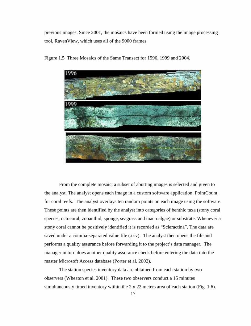
Representative images for all transects are frame-grabbed. These images form a

mosaic of each transects. Figure 1.5 shows three mosaics of the same transect from the

years 1996, 1999 and 2004. The stony coral seen in these transects is Acropora palmata.

These mosaics are then used to obtain point count data. From 1996 to 2000, the

procedure of forming the mosaic is as follows: About 120 frames are digitized to cover

the complete coverage of the sea floor since there is a considerable overlap of the video

frames. The subset of frames is grabbed based on swim speed. From these only about 60

are selected by a trained analyst so that there is no more than 15% overlap with the

17

previous images. Since 2001, the mosaics have been formed using the image processing

tool, RavenView, which uses all of the 9000 frames.

Figure 1.5 Three Mosaics of the Same Transect for 1996, 1999 and 2004.

From the complete mosaic, a subset of abutting images is selected and given to

the analyst. The analyst opens each image in a custom software application, PointCount,

for coral reefs. The analyst overlays ten random points on each image using the software.

These points are then identified by the analyst into categories of benthic taxa (stony coral

species, octocoral, zooanthid, sponge, seagrass and macroalgae) or substrate. Whenever a

stony coral cannot be positively identified it is recorded as “Scleractina”. The data are

saved under a comma-separated value file (.csv). The analyst then opens the file and

performs a quality assurance before forwarding it to the project’s data manager. The

manager in turn does another quality assurance check before entering the data into the

master Microsoft Access database (Porter et al. 2002).

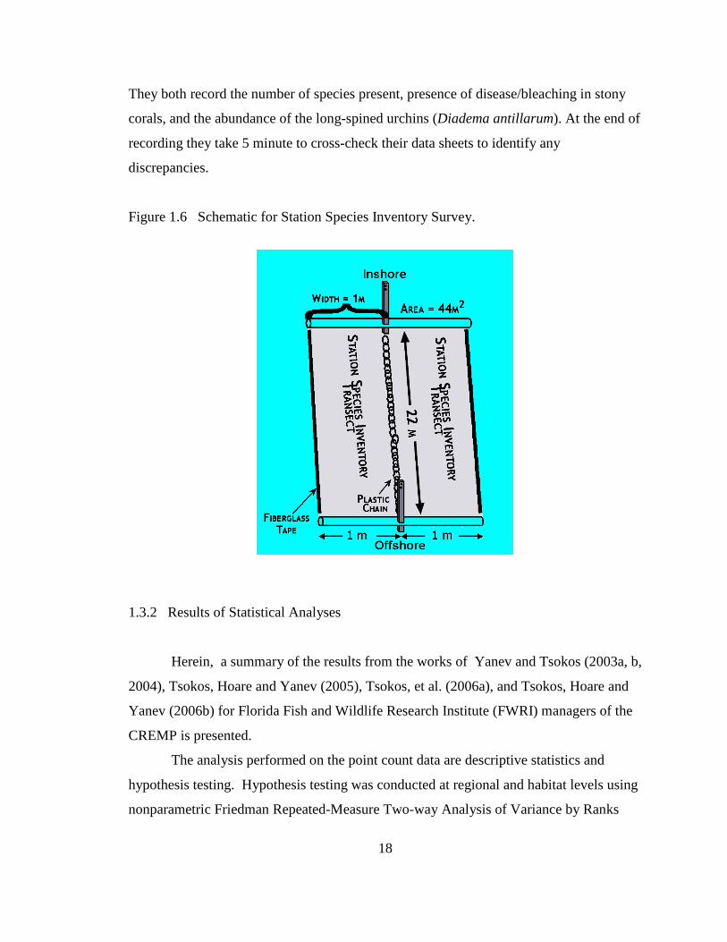
The station species inventory data are obtained from each station by two

observers (Wheaton et al. 2001). These two observers conduct a 15 minutes

simultaneously timed inventory within the 2 x 22 meters area of each station (Fig. 1.6).

18

They both record the number of species present, presence of disease/bleaching in stony

corals, and the abundance of the long-spined urchins (Diadema antillarum). At the end of

recording they take 5 minute to cross-check their data sheets to identify any

discrepancies.

Figure 1.6 Schematic for Station Species Inventory Survey.

1.3.2 Results of Statistical Analyses

Herein, a summary of the results from the works of Yanev and Tsokos (2003a, b,

2004), Tsokos, Hoare and Yanev (2005), Tsokos, et al. (2006a), and Tsokos, Hoare and

Yanev (2006b) for Florida Fish and Wildlife Research Institute (FWRI) managers of the

CREMP is presented.

The analysis performed on the point count data are descriptive statistics and

hypothesis testing. Hypothesis testing was conducted at regional and habitat levels using

nonparametric Friedman Repeated-Measure Two-way Analysis of Variance by Ranks

19

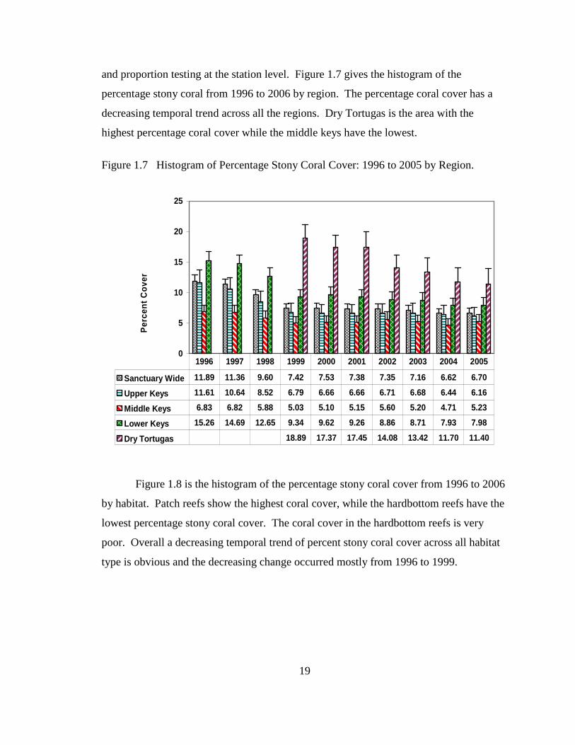
and proportion testing at the station level. Figure 1.7 gives the histogram of the

percentage stony coral from 1996 to 2006 by region. The percentage coral cover has a

decreasing temporal trend across all the regions. Dry Tortugas is the area with the

highest percentage coral cover while the middle keys have the lowest.

Figure 1.7 Histogram of Percentage Stony Coral Cover: 1996 to 2005 by Region.

0

5

10

15

20

25

Per

cent

Cov

er

Sanctuary Wide 11.89 11.36 9.60 7.42 7.53 7.38 7.35 7.16 6.62 6.70

Upper Keys 11.61 10.64 8.52 6.79 6.66 6.66 6.71 6.68 6.44 6.16

Middle Keys 6.83 6.82 5.88 5.03 5.10 5.15 5.60 5.20 4.71 5.23

Lower Keys 15.26 14.69 12.65 9.34 9.62 9.26 8.86 8.71 7.93 7.98

Dry Tortugas 18.89 17.37 17.45 14.08 13.42 11.70 11.40

1996 1997 1998 1999 2000 2001 2002 2003 2004 2005

Figure 1.8 is the histogram of the percentage stony coral cover from 1996 to 2006

by habitat. Patch reefs show the highest coral cover, while the hardbottom reefs have the

lowest percentage stony coral cover. The coral cover in the hardbottom reefs is very

poor. Overall a decreasing temporal trend of percent stony coral cover across all habitat

type is obvious and the decreasing change occurred mostly from 1996 to 1999.

20

Figure 1.8 Histogram of Percent Stony Coral Cover: 1996 to 2005 by Habitat.

0

5

10

15

20

25

Per

cent

Cov

er

Patch Reefs 19.98 18.80 17.87 15.48 15.96 15.70 15.59 15.32 14.32 15.33

Deep Reefs 6.73 6.78 4.46 3.74 3.75 3.71 3.60 3.51 2.89 3.00

Shallow Reefs 12.12 11.55 9.15 5.48 5.51 5.19 5.45 5.17 4.97 4.30

Hardbottom 1.92 1.92 1.56 1.79 1.38 1.89 1.18 1.31 0.94 1.20

1996 1997 1998 1999 2000 2001 2002 2003 2004 2005

Table 1.4 gives the result of hypothesis testing performed at regional and habitat

levels to check if there exists any statistical change in mean stony coral cover over the

years from 1999 to 2005. We tested the null hypothesis that the mean stony coral cover

is the same in all years from 1999 to 2005 as opposed to the alternative hypothesis that

the mean stony coral cover is different in at least one of the years. The results show that

there was a statistical significant change in mean stony coral cover in all the different

types of reefs at 0.05α = . This means that there exists statistically at least one year

whose mean stony coral cover is different than the rest of the years. By region, the upper

keys and middle keys showed no statistical significant change in mean stony coral cover

at 0.05α = . This means that statistically there is no evidence that the mean stony coral

cover is different for any of the years tested. But there is statistical evidence that there

exist at least one year whose mean stony coral cover is different than the rest of the years

in the lower keys and the sanctuary.

21

Table 1.4 Hypothesis Testing for Change in Mean Stony Coral Cover: 1999 to 2005.

Region and Statistical Significance Habitat 0.05α =

Sanctuary Yes Upper Keys No Middle Keys No Lower Keys Yes Dry Tortugas Yes Patch Reefs Yes Deep Reefs Yes

Shallow Reefs Yes Hardbottom Yes

We tested for statistically significant change in stony coral cover per station for

consecutive years (2003 vs. 2002, 2003 vs. 2004 and 2004 vs. 2005). The null hypothesis

that the stony coral proportion in one year is the same as in the other year as oppose to

the alternative hypothesis that they differ was tested. Figure 1.9 shows the pie chart for

the percentage number of stations that showed statistical significant change (loss, gain or

no change) for the three pairs of years tested. The number of stations that lost stony coral

cover in consecutive years have fallen in 2005 vs. 2004 as compared to the other pairs of

years. The number of stations tested that showed a gain in stony coral cover fell in 2004

vs. 2003 from the pair in 2003 vs. 2002 but increased in 2005 vs. 2004. In the case of

testing for no change in stony coral cover, the percentage was the same for pairs 2003 vs.

2002 and 2005 vs. 2004 but higher in 2004 vs. 2003.

22

Figure 1.9 Percentage Change in Stony Coral Cover by Station.

2003 vs 2002

67%

10%

23%

2004 vs 2003

23%

6%

71%

2005 vs 2004

17%

16%

67%

Loss Gain Equal

The point count data were also used in calculating the Shannon-Wiener diversity

index. Shannon-Wiener diversity index is described as:

ln ln1' ln

1

sn n f fi is iH p pi i ni

− ∑=∑= − ==

= (1.1)

where /i ip f n= is the proportion of points where the i th stony coral species is identified,

if is the abundance of the ith stony coral species, s is the number of species present and

n is the total abundance of all species in the sample. The Shannon-Wiener diversity

index is a measure of the how diverse a habitat is by considering both the species present

and their abundance. Using equation (1.1) and the Jackknifing method (explained further

in section 3.2), we estimate the Shannon-Wiener diversity index and construct the 95%

23

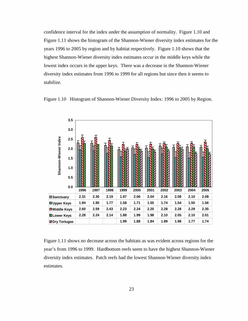
confidence interval for the index under the assumption of normality. Figure 1.10 and

Figure 1.11 shows the histogram of the Shannon-Wiener diversity index estimates for the

years 1996 to 2005 by region and by habitat respectively. Figure 1.10 shows that the

highest Shannon-Wiener diversity index estimates occur in the middle keys while the

lowest index occurs in the upper keys. There was a decrease in the Shannon-Wiener

diversity index estimates from 1996 to 1999 for all regions but since then it seems to

stabilize.

Figure 1.10 Histogram of Shannon-Wiener Diversity Index: 1996 to 2005 by Region.

0.0

0.5

1.0

1.5

2.0

2.5

3.0

3.5

Sha

nnon

-Wie

ner

Inde

x

Sanctuary 2.31 2.30 2.19 1.97 2.06 2.04 2.16 2.08 2.10 2.08

Upper Keys 1.94 1.90 1.77 1.58 1.71 1.55 1.74 1.54 1.50 1.56

Middle Keys 2.60 2.59 2.43 2.23 2.24 2.25 2.28 2.28 2.29 2.35

Lower Keys 2.28 2.24 2.14 1.88 1.99 1.98 2.10 2.05 2.10 2.01

Dry Tortugas 1.99 1.88 1.84 1.89 1.98 1.77 1.74

1996 1997 1998 1999 2000 2001 2002 2003 2004 2005

Figure 1.11 shows no decrease across the habitats as was evident across regions for the

year’s from 1996 to 1999. Hardbottom reefs seem to have the highest Shannon-Wiener

diversity index estimates. Patch reefs had the lowest Shannon-Wiener diversity index

estimates.

24

Figure 1.11 Histogram of Shannon-Wiener Diversity Index: 1996 to 2005 by Habitat.

0.0

0.5

1.0

1.5

2.0

2.5

3.0

3.5

Sha

nnon

-Wie

ner

Inde

x

Patch Reefs 1.85 1.77 1.74 1.67 1.85 1.83 1.92 1.85 1.88 1.89

Deep Reefs 2.37 2.35 2.22 1.90 1.95 2.07 2.08 2.13 2.13 2.01

Shallow Reefs 2.12 2.12 2.12 1.94 1.98 1.92 2.07 1.98 1.94 1.95

Hardbottom 1.93 2.50 2.49 2.24 2.65 2.49 2.04 2.15 2.45 2.39

1996 1997 1998 1999 2000 2001 2002 2003 2004 2005

Figure 1.12 shows the Shannon-Wiener diversity index estimate plus the 95%

confidence interval of the true Shannon-Wiener diversity index of the Sanctuary region

from 1996 to 2005. To create the confidence interval we used the jackknifing method.

From this method, we were able to obtain pseudovalues which are used to estimate the

Shannon-Wiener diversity index and to carryout inferences on the true value of the

Shannon-Wiener diversity index. In constructing the 95% confidence interval of the true

value of the Shannon-Wiener diversity index, we assume that the underlying probability

structure of the pseudovalues is the normal distribution. One can see that there was a

decrease in the Shannon-Wiener diversity index from 1996 to 1999; there was a slight

increase from 1999 to 2002, and then it seems to stabilize.

25

Figure 1.12 95% Confidence Interval of the Shannon-Wiener Diversity Index for the

Sanctuary Region.

1.00

1.50

2.00

2.50

3.00S

hann

on-W

iene

r In

dex

Jacknife Estimate 2.31 2.30 2.19 1.97 2.06 2.04 2.16 2.08 2.10 2.08

1996 1997 1998 1999 2000 2001 2002 2003 2004 2005

For the species inventory data, we performed hypothesis testing and constructed a

95% confidence interval for each species of stony coral species present. The null

hypothesis was that the number of stations where the stony coral species was present

didn’t change for the years tested. We considered the following time periods: 2002-03 vs.

1996-01, 2003-04 vs. 1996-02, and 2004-05 vs. 1996-03. Table 1.5 shows the summary

of the results for the hypothesis testing for all three time periods. It gives the number of

species that had statistical significant negative, positive or no change in the number of

stations.

26

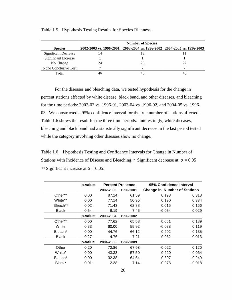
Table 1.5 Hypothesis Testing Results for Species Richness.

Number of Species Species 2002-2003 vs. 1996-2001 2003-2004 vs. 1996-2002 2004-2005 vs. 1996-2003

Significant Decrease 14 13 11 Significant Increase 1 1 1

No Change 24 25 27 None Conclusive Test 7 7 7

Total 46 46 46

For the diseases and bleaching data, we tested hypothesis for the change in

percent stations affected by white disease, black band, and other diseases, and bleaching

for the time periods: 2002-03 vs. 1996-01, 2003-04 vs. 1996-02, and 2004-05 vs. 1996-

03. We constructed a 95% confidence interval for the true number of stations affected.

Table 1.6 shows the result for the three time periods. Interestingly, white diseases,

bleaching and black band had a statistically significant decrease in the last period tested

while the category involving other diseases show no change.

Table 1.6 Hypothesis Testing and Confidence Intervals for Change in Number of

Stations with Incidence of Disease and Bleaching. * Significant decrease at α = 0.05

** Significant increase at α = 0.05.

p-value Percent Presence 95% Confidence Interval 2002-2003 1996-2001 Change in Number of Stations

Other** 0.00 87.14 61.59 0.193 0.318 White** 0.00 77.14 50.95 0.190 0.334 Bleach** 0.02 71.43 62.38 0.015 0.166

Black 0.64 6.19 7.46 -0.054 0.029 p-value 2003-2004 1996-2002

Other** 0.00 77.62 65.58 0.051 0.189 White 0.33 60.00 55.92 -0.038 0.119

Bleach* 0.00 44.76 66.12 -0.292 -0.135 Black 0.27 4.76 7.21 -0.062 0.013

p-value 2004-2005 1996-2003 Other 0.20 72.86 67.98 -0.022 0.120 White* 0.00 43.33 57.50 -0.220 -0.064 Bleach* 0.00 32.38 64.64 -0.397 -0.249 Black* 0.01 2.38 7.14 -0.078 -0.018

27

Figure 1.13 shows the percentage number of stations with incidence of white

disease, black band, bleaching and other diseases from 1996 to 2005. Figure 1.13

confirms there is a decrease in the white diseases, bleaching and black band incidence per

stations in the last three years. But at the same time the incidence of white diseases,

bleaching and other disease remain high. Figures 1.13 also show that there may be some

cyclic trend, which may become more obvious as more data are obtained over the coming

years.

Figure 1.13 Stations with Incidence of Disease and Bleaching, 1996- 2005.

0

10

20

30

40

50

60

70

80

90

100

Other 11.43 43.81 64.76 87.62 71.43 90.48 89.52 84.76 70.48 75.24

White 4.76 44.76 65.71 64.76 53.33 72.38 85.71 68.57 51.43 35.24

Bleach 51.43 59.05 80.95 78.10 66.67 38.10 88.57 54.29 35.24 29.52

Black 6.67 3.81 18.10 4.76 8.57 2.86 5.71 6.67 2.86 1.90

1996 1997 1998 1999 2000 2001 2002 2003 2004 2005

Per

cent

of S

tatio

ns

Affe

cted

The main focus of this dissertation is to contribute to the statistical analysis of the

stony coral data obtained from the coral reef evaluation and monitoring project

(CREMP), the project is described in section 1.3. It is imperative to be able to

statistically investigate the true status of the stony coral cover in a monitoring project.

The analysis of the CREMP data by the works of Yanev et al. (2003a, b, 2004) and

28

Tsokos et al. (2005, 2006a, b) was limited to only descriptive and non-parametric

analysis when analyzing the percent coral cover. This being a first approximation

technique, it is possible to analyze the data with more powerful analysis techniques if the

underlying probability structure of the data can be identified. In the case of the Shannon-

Wiener diversity index using the jackknifing method possesses a limitation in that the

pseudovalues, whose average is used as an estimate for the Shannon-Wiener diversity

index, are assumed to follow a normal distribution. This assumption is used in the

construction of the 95% confidence interval of the true Shannon-Wiener diversity index.

These two and other concerns addressed in this study.

1.4 Focus of Chapter Two

To accomplish the objectives of CREMP, a thorough and complete analysis of the

statistical properties of the stony coral cover proportions is vital. We address these

objectives in this chapter. We shall analyze the stony coral cover proportions data of all

the stations within the Sanctuary Region from 1996 to 2006. The main purpose is to

identify the probability density function (pdf) of stony coral cover proportions in the

Florida Keys and to investigate if the reported mean values of the coral cover in the

Technical Reports (Yanev et al. 2003a, b, 2004, Tsokos et al. 2005, 2006a) are good

estimates of the true mean stony coral cover of the sanctuary region of CREMP over the

years of the project. In addition, the 90% and 95% confidence intervals for the true

median and the true mean of the population stony coral cover are given. A comparison of

the “a proposed method” and the “naïve method” will be made with respect to the median

confidence intervals. Finally, comparisons of the mean confidence interval obtained

using the naïve method, the Cox method and a proposed method are also made.

1.5 Focus of Chapter Three

A focus of this chapter is to investigate the applicability of the normal probability

distribution assumption made on the pseudovalues obtained from the jackknifing

29

procedure for the Shannon-Wiener diversity index used in the works presented by Yanev

et al. (2003a, b, 2004), and Tsokos et al. (2005, 2006a) for the CREMP. The normality

assumption was made when we constructed the 95% confidence interval for the true

Shannon-Wiener diversity indices for the entire sanctuary for years from 1996 to 2005.

The validity of normality with respect to the 12 stations in the Dry Tortugas area of the

CREMP is also investigated. The accuracy of the confidence interval is investigated

using the bootstrapping resampling procedure. Testing for normality of the pseudovalues

is done using the Shapiro-Wilks normality test.

We also propose in this chapter that the underlying probability structure of the

species abundance be found if possible so that it gives a better approximation of the true

diversity index. Once the probability distribution of the species abundance is fitted then

we can use the probability distribution instead of the species abundance data in obtaining

as estimate of the true Shannon-Wiener diversity index or true Simpson’s diversity index

for the entire sanctuary from 1996 to 2006. The Shannon-Wiener diversity index for the

two-parameter lognormal probability distribution is obtained from literature under

Shannon entropy. We solved the Simpson’s diversity index for the two-parameter

lognormal probability distribution in this study.

1.6 Focus of Chapter Four

The aim of this chapter is to develop the best possible estimate of the probability

distribution of the jackknifing pseudovalues for the sanctuary using the nonparametric

kernel density method. Once the best kernel density estimate is obtained, a comparison

with the parametric approach under the normal assumption will be made. We compare

the mean, standard deviation, standard error and the 95% confidence interval of the true

mean.

30

1.7 Focus of Chapter Five

The aim of this chapter is to develop a predictive statistical model of stony coral

cover proportions. Such a model would identify the attributable variables that influence

the stony coral cover data of the lower Florida Keys. Having the attributable variables for

different coral reef areas, we would be able to predict an estimate of the stony coral cover

of that area.

31

Chapter 2

Parametric Analysis of Stony Coral Cover From the Florida Keys

2.1 Introduction

Coral reef habitats have been, and continue to be, the subject of many research

studies. The main goals of these studies are to investigate and document the health status

of these habitats. Unfortunately many of the published studies are short in duration and

narrow in scope. Such limitations have posed many difficulties in analyzing existing data

for temporal or spatial differences and trends. The main difficulty is a limited sample

size. Small sample size limits the investigation of the underlying probability distribution

of such data. Such information is invaluable in parametric analysis. If the probability

distribution function is not easily identified, the tendency is to use non-parametric

analysis to analyze the data. Lirman et al. (2007) used Kruskal-Wallis test to compare

the percent cover of eight main benthic categories among his different survey methods.

Yanev et al. (2003a, b, 2004) and Tsokos et al. (2005, 2006a) used the nonparametric

Friedman Repeated-Measure Two-way Analysis of Variance by Ranks to detect the

differences in percent stony coral cover over the years. Non-parametric tests are best

used when the distribution of the data is unknown or it cannot be safely detected;

however, non-parametric tests are less powerful than parametric tests. On the other hand,

if parametric analyses are prematurely used, they have less power than the non-

parametric analyses. While scientists have used data transformations to employ

parametric analysis, the most widely used parametric analysis seems to be ANOVA,

which assumes normality, homogeneity of variance, and random independent samples.

Many follow suggested transformations given by various authors (Sokal and Rohlf 1995,

32

Zar 1996, Hayek and Buzas 1997, Krebs 1999) to achieve the assumptions required for

parametric analysis. Rogers, Gilnack and Fitz (1983), Carleton and Done (1995),

Murdoch and Aronson (1999), and Wielgus et al. (2004) used the arcsine transformation

to be able to use ANOVA. Brown et al. (2004) used the arcsine-square root

transformation to be able to use the paired t-test. Pante et al. (2007), on the other hand,

used the log transformation to apply the t-test to test for change in percent cover of stony

coral between 1991 and 2004. It is imperative to know the probability distribution of

percent coral cover. This would ensure that the proper statistical test is employed and

ecosystem managers could make more meaningful inferences and better managerial

decisions.

With the development of convenient reliable sampling techniques, such as

videography, monitoring programs such as CREMP, Coral Reef Assessment and

Monitoring Program (CRAMP) in Hawai’I, and the Australian Institute of Marine

Science (AIMS) monitoring program are sampling larger areas of reefs over longer

periods of time. Monitoring of coral reefs to estimate coral cover through camera and

video technology (Pavlov et al. 2004, Wielgus et al. 2004) at small scale is becoming

more common. These studies use the point count method on the photos or video-frames

to obtain coral cover values. Many studies have documented the effectiveness and

disadvantages of videography as a coral sampling method. Carleton and Done (1995)

and Lirman et al. (2007) concluded that proper video sampling procedure provides a

quantitative measure of spatial variability and temporal change in benthic communities

on coral reefs. This provides a cost saving method for sampling larger areas and produces

a permanent record of the sampling sites as shown in Figure 1.5 (see Chapter 1). It can

be seen that Acropora palmata was thriving in this transect from a CREMP station in

1996 but was nonexistent in 1999. The mosaic shows the return of this very important

stony coral species in 2004. One limitation of videography is the taxonomic resolution.

As a result, it does not give a good estimate of the presence of rare species. Lirman et al.

(2007) also concluded that the video-mosaic did have problems in revealing juvenile

corals. Nevertheless, for a monitoring project whose focus is to document temporal

change over a large area, videography is a time saving method that is economically

33

feasible. It is still important to identify the probabilistic structure of percent stony coral

cover. Larger samples will facilitate the investigation of the probability distribution

function of percent stony coral cover.

The data used in this study comes from the Florida Keys Coral Reef Evaluation

and Monitoring Project (CREMP). To accomplish the objectives of the CREMP a

thorough and complete analysis of the statistical properties of the stony coral cover

proportions is vital. We address these objectives in this study. We shall analyze the

stony coral cover proportions data of all the stations within the Sanctuary Region from

1996 to 2006. The main purpose is to identify the probability density function (pdf) of

stony coral cover proportions in the Florida Keys and to investigate if the reported mean

values of coral cover in the Technical Reports (Yanev et al. 2003a, b, 2004, Tsokos et al.

2005, 2006a) are good estimates of the true mean stony coral cover of the sanctuary

region of the CREMP over the years of the project. In addition, the 90% and 95%

confidence intervals for the true median and the true mean of the stony coral cover are

given. A comparison of the “proposed method” and the “naïve method” will be made

with respect to the median confidence intervals. Finally, comparisons of the mean

confidence interval obtained using the naïve method, the Cox method and a proposed

method are also made.

2.2 Descriptive Statistic: Proportion of Stony Coral Cover

The stony coral cover proportions are obtained from the point count method used

by the CREMP. The mosaics used in the point count method come from 37 sites over the

Florida Keys. These include transects from 105 stations for the years 1996 to 2005 and

103 stations in 2006. The data demonstrate right skewness and display leptokurtic

behavior as shown by the histogram given in Figure 2.1. The stony coral cover

proportion data for the other years from 1996 to 2005 display similar histograms as 2006,

(Fig. 2.1).

34

Figure 2.1 Histogram for the Stony Coral Cover Proportions for 2006.

0

10

20

30

40

50

0.00 0.05 0.10 0.15 0.20 0.25 0.30

Per

cent

0

10

20

30

40

50

0.00 0.05 0.10 0.15 0.20 0.25 0.30

Per

cent

Table 2.1 gives the descriptive statistics of the stony coral cover proportions from

1996 to 2006. A skewness measure that is greater that zero means the data are skewed to

the right and a value less than zero means it is skewed to the left. Thus, Table 2.1

presents further evidence that the stony coral cover proportions data from 1996 to 2006

displays right skewness as the skewness values range from 1.17 to 1.81. A kurtosis

measure greater than zero means the distribution displays leptokurtic behavior and a

value less than zero means the distribution displays a platykurtic behavior. A kurtosis

value of zero means the distribution displays mesokurtic behavior. Leptokurtic behaviors

in the stony coral proportions data are also evident from Table 2.1, since the kurtosis

values are all greater than zero.

35

Table 2.1 Descriptive Statistics for Proportion Stony Coral Cover.

The boxplots, shown below by Figure 2.2, display the spread of the stony coral

cover proportions data from 1996 to 2006. The boxplots show that many of the data

values are found between 0 and 0.1. The whiskers of the boxplots are longer towards the

larger values, further evidence that the distribution of the stony coral cover proportions

data are skewed to the right. Thus, any attempt at identifying a probability density

function for these data sets must be one that takes into consideration right skewness.

1996 1997 1998 1999 2000 2001 2002 2003 2004 2005 2006 Mean 0.119 0.114 0.096 0.074 0.075 0.074 0.073 0.072 0.066 0.067 0.061 Median 0.091 0.089 0.057 0.047 0.047 0.041 0.045 0.042 0.035 0.039 0.030 Std Error 0.010 0.009 0.009 0.007 0.008 0.007 0.008 0.008 0.007 0.008 0.008 Std Dev 0.101 0.094 0.092 0.076 0.078 0.076 0.080 0.081 0.076 0.079 0.079 Kurtosis 0.988 1.084 1.734 1.353 1.485 1.924 2.211 2.361 2.871 2.019 2.088 Skewness 1.171 1.236 1.473 1.487 1.509 1.600 1.707 1.767 1.866 1.746 1.771

36

Figure 2.2 Boxplots for Stony Coral Cover Proportion Data from 1996 to 2006.

1996 1997 1998 1999 2000 2001 2002 2003 2004 2005 2006

0

0.1

0.2

0.3

0.4

0.5

Year

Pro

prot

ion

1996 1997 1998 1999 2000 2001 2002 2003 2004 2005 2006

0

0.1

0.2

0.3

0.4

0.5

Year

Pro

prot

ion

2.3 Procedure in Fitting a Three Parameter Lognormal Probability Density Function

In this section we shall introduce the theory used in estimating the parameters of

the 3-parameter lognormal probability density function and evaluating its fit to the

subject data.

A random variable has the three parameter lognormal probability distribution

function if its probability density function is given by:

22 1/2 1 1 ln( )

(2 ) ( ) exp( ) 2

0

xx if x

f x

if x

θ µπσ θ θσ

θ

− − − − − − > = ≤

, (2.1)

is the threshold parameter, is the scale parameter and is the shape parameter.

37

2.3.1 Maximum Likelihood Estimation Procedure

The method of maximum likelihood estimator (MLE) is considered to be more

robust than other methods, such as methods based on moments or quantiles. In general

MLE possesses many desirable statistical properties such as consistency, invariant,

asymptotical normality, efficiency, and sufficiency. The MLE method was the method of

choice to approximate the parameters of the three parameter lognormal probability

density function (equation (2.1)) considered here.

Even though the MLE for the three parameter lognormal pdf seems not to have

the usual asymptotic efficiency, Calitz (1973) concluded that the variance is much

smaller than that of the estimators based on moments and quantiles, and is close to the

theoretical asymptotic variance with large samples. Through a Monte Carlo study Calitz

(1973) compared the estimates using the methods of MLE as described by Cohen (1951) ,

method of generalized moments and the method of quantiles for 50 samples of size 100

with varying parameters. Calitz (1973) concluded that the method of MLE is much better

than the other methods and that it should be considered as the prime method for

estimating the parameters of the three parameter lognormal distribution. He strongly

suggested using the procedure as shown by Cohen (1951) since other studies did not have

success with alternative procedures. Cohen (1951) was one of the first to suggest the use

of a local MLE now known as the local maximum likelihood estimator (LMLE).

The MLE of the three unknown parametersθ , µ and 2σ maximizes the

likelihood function of a random sample. The likelihood function, 21( ,..., ; , , )nL x x θ µ σ , of

the random sample consisting of n independent observations 1( ,..., )nx x x= from

n independent random variables 1( ,..., )nX X X= each with the three parameter lognormal

probability density function ( ( )f x ) is as follows:

38

21( ,..., ; , , )nL x x θ µ σ =

22 /2 1

11

ln( )1(2 ) ( ) exp ,

2

0 .

n nn i

i iii

i

xx if all x

if some x

θ µπσ θ θσ

θ

− −

==

− − − − > ≤

∑∏ (2.2)

Without loss of generality, assume that theix s are in increasing order, such that 1x is the

smallest data value. Hill (1963) has shown that arbitrarily large likelihoods can be

achieved by allowing θ to converge on1x . Thus, the true maximum likelihood estimates

should be 1ˆ xθ = , µ = −∞ and 2σ = ∞ regardless of the sample. This leads to

inadmissible estimates for the parameters. However, Cohen (1951) had already shown

that a localized estimate of the threshold parameter θ was sufficient in the identification

of the three parameter lognormal. Calitz (1973), Cohen and Whitten (1980), and Chen

(2006) and others have since investigated the validity of the estimates from such

procedure. Cohen’s procedure (Cohen 1951) identifies the LMLE for the threshold

parameter θ and then finds the MLE for the parameters µ and σ . To find these

estimates we take the logarithm of the likelihood function 21( ,..., ; , , )nL x x θ µ σ , equation

(2.2), and then set the partial derivatives with respect to θ , µ and σ equal to zero. The

log-likelihood function is given by:

21ln ( ,..., ; , , )nL x x θ µ σ =

22

1 1

1ln(2 ) ln ln( ) (ln( ) ) .

2 2

n n

i ii i

nn x xπ σ θ θ µ

σ= =

− − − − − − −∑ ∑ (2.3)

The partial derivatives give:

21

ln 1(ln( ) ) 0

n

ii

Lx θ µ

µ σ =

∂ = − − =∂ ∑ , (2.4)

23

1

ln 1(ln( ) ) 0

n

ii

L nx θ µ

σ σ σ =

∂ = − + − − =∂ ∑ (2.5)

and

39

21 1

ln( )ln 1 10

n ni

i ii i

xL

x x

θ µθ σ θ θ= =

− −∂ = + =∂ − −∑ ∑ . (2.6)

Solving the first two equations (2.4) and (2.5), gives the estimates for µ and 2σ ,

respectively:

1

1 ˆˆ ln( )n

ii

xn

µ θ=

= −∑ (2.7)

and

2

2 2

1 1

1 1ˆ ˆˆ (ln( )) ln( )n n

i ii i

x xn n

σ θ θ= =

= − − −

∑ ∑ . (2.8)

Substituting equations (2.7) and (2.8) in equation (2.6), we have

2

1

1 2

1 1 1

1 ˆln(ˆ ˆ ˆ( ) ln( ) (ln( ))n

ii

n n n

i i ii i i

xn

x x x θθ θ θ=

−

= = =

+ −

− − − − ∑∑ ∑ ∑

1

ˆln( )0.

ˆ

ni

i i

xn

x

θθ=

−− =−∑ (2.9)

Equation (2.9) is solved iteratively for the local maximum likelihood estimate (LMLE),

θ , for θ . Only admissible roots for which θ is less than 1x are considered. According to

Cohen and Whitten (1980), usually only one such root is found. In cases where there are

more than one admissible root, the root that gives the closest agreement between the

expected value of the three parameter lognormal distribution and the mean of the data, is

taken as the estimate. Once the estimate θ is found then the estimates of µ and 2σ are

found using equations (2.7) and (2.8). Cohen and Whitten (1980) concluded that the

LMLE is suitable whenever the skewed value of the data is greater than one and

suggested other modified maximum likelihood estimators when the data has a skewed

value less than one.

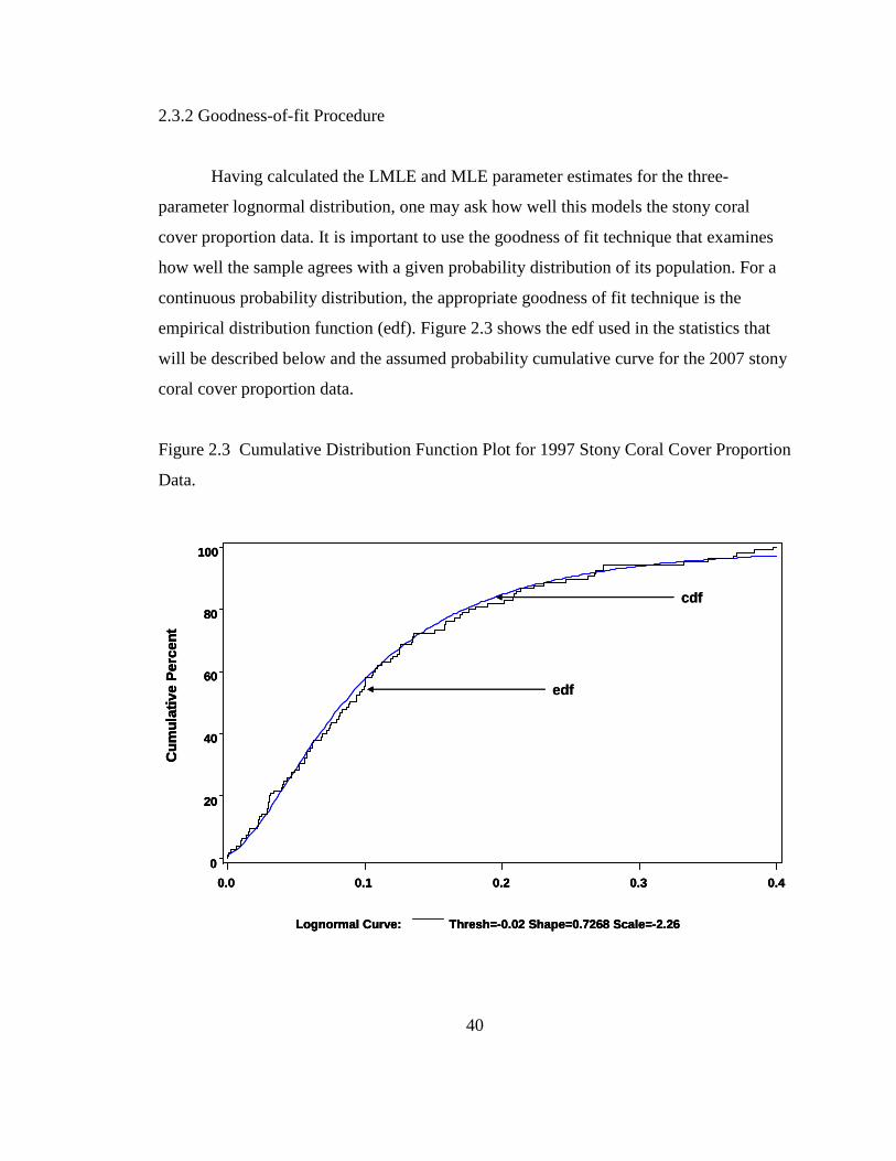
40

2.3.2 Goodness-of-fit Procedure

Having calculated the LMLE and MLE parameter estimates for the three-

parameter lognormal distribution, one may ask how well this models the stony coral

cover proportion data. It is important to use the goodness of fit technique that examines

how well the sample agrees with a given probability distribution of its population. For a

continuous probability distribution, the appropriate goodness of fit technique is the

empirical distribution function (edf). Figure 2.3 shows the edf used in the statistics that

will be described below and the assumed probability cumulative curve for the 2007 stony

coral cover proportion data.

Figure 2.3 Cumulative Distribution Function Plot for 1997 Stony Coral Cover Proportion

Data.

Lognormal Curve: Thresh=-0.02 Shape=0.7268 Scale=-2. 26

0

20

40

60

80

100

0.0 0.1 0.2 0.3 0.4

Cum

ulat

ive

Per

cent

cdf

edf

Lognormal Curve: Thresh=-0.02 Shape=0.7268 Scale=-2. 26

0

20

40

60

80

100

0.0 0.1 0.2 0.3 0.4

Cum

ulat

ive

Per

cent

Lognormal Curve: Thresh=-0.02 Shape=0.7268 Scale=-2. 26

0

20

40

60

80

100

0.0 0.1 0.2 0.3 0.4

Cum

ulat

ive

Per

cent

cdf

edf

41

The edf is a step function that takes a step of height 1

n at each observation of the sample.

The edf statistic measures the differences between the edf and the given cumulative

distribution function (cdf) values whose parameters are either known or unknown (which

are estimated from the sample). The edf statistic is based on the differences between the

edf from the proportion stony coral cover and the three-parameter lognormal distribution,

equation 2.1, with estimates for the threshold, scale and shape parameters from the

sample. The edf is defined for a set of n independent observations 1,..., nX X with a

common cumulative distribution function ( )F x such as the one from the three-parameter

lognormal distribution. Suppose that the sample of size n is arranged in increasing order

(1) (2) ( )... nX X X< < < , then the empirical distribution function ( )nF x is defined as

follows:

(1)( ) 0,nF x x X= <

( ) ( 1)( ) , 1,..., 1n i i

iF x X x X i n

n += ≤ ≤ = −

( )( ) 1, .n nF x X x= ≤

At any valuex , ( )nF x is the proportion of observations that are less than or equal tox .

( )F x is the theoretical probability of an observation that is less than or equal to x . It is

expected that ( )nF x estimates ( )F x which is a consistent estimator of ( )F x as n → ∞

meaning that ( ) ( ) 0PnF x F x− → . In order to compute the edf statistics, the probability

integral transformation ( )U F X= is used. If ( )F X is the cdf of X , the random variable

U is uniformly distributed between 0 and 1.

There are several goodness of fit tests that are based on edf. They are based on the

vertical differences between ( )nF x and ( )F x . These tests are usually divided into two

different classes: the supremum and the quadratic. We use the well known Kolmogorov-

Smirnov statistic D , which is in the supremum class and from the quadratic class, we use

both the Cramer-von Mises statistic 2W and the Anderson-Darling statistic 2A .

42

The Kolmogorov-Smirnov statistic D is defined as:

sup ( ) ( ) max( , ).x nD F x F x D D+ −= − =

This statistic is calculated by taking the maximum value of D+ and D− . D+ is the largest

vertical difference between the edf and the cdf whenever the edf is greater than the cdf.

D− is the largest vertical difference between the edf and the cdf whenever the edf is less

than the cdf.

( )maxi i

iD U

n+ = −

( )

1maxi i

iD U

n− − = −

In the case of the quadratic class the general statistic is defined as:

2( ( ) ( )) ( ) ( )nQ n F x F x x dF xψ∞

−∞

= −∫

where ( )xψ is a suitable function which gives weights to the squared difference

2( ( ) ( ))nF x F x− . For the Cramer-von Mises statistic 2W , ( )xψ is equal to 1.

The Cramer-von Mises statistic 2W is therefore:

2 2( ( ) ( )) ( ) ( ).nW n F x F x x dF xψ∞

−∞

= −∫

It is computed as:

2

2( )

1

2 1 1.

2 12

n

ii

iW U

n n=

− = − +

∑

For the Anderson-Darling statistic2A , ( )xψ is equal to ( ) 1( ) 1 ( )F x F x

− − .

The Anderson-Darling statistics 2A is:

( ) 12 2( ( ) ( )) ( ) 1 ( ) ( ).nA n F x F x F x F x dF x∞

−

−∞

= − − ∫

It is computed using:

2( ) 1

1(2 1)(ln ln(1 )) .i n iA n i U U

n = − = − − − + − ∑

43

It is very important to note that if the parameters are estimated from the sample,

the edf techniques give different p-values than if the parameters are known. When the

true parameters are known, the ( )iU follow the uniform distribution but that is not the case

when the parameters are estimated from the sample. In such a case, the formulae are the

same but the distribution of the edf statistics will depend on the distribution being tested,

the parameters estimated, the method of estimation and the sample size. To obtain the

critical values, simulation is used. Many tables of critical value have been created, e.g.

Stephens (1986) and Chen (2006). The null hypothesis for general goodness-of-fit tests

based on edf is that the random sample of n , X -values comes from( )F x . The alternative

hypothesis is that the random sample of n , X -values do not come from( )F x . Chen

(2006) showed that the modified Kolmogorov-Smirnov statistic nD , the Cramer-von

Mises statistic 2W and the Anderson-Darling statistic 2A are very accurate goodness-of-

fit tests for the three-parameter lognormal when the estimates are found using the LMLE

and the MLE estimators. He concluded that Anderson-Darling statistic 2A was the most

powerful edf test followed by Cramer-von Mises statistic 2W and then the modified

Kolmogorov-Smirnov statistic nD for the three parameter lognormal distribution. Even

though the Anderson-Darling statistic was the most powerful of the three, the other two

functioned very well. The null hypothesis of these tests is that the edf and cdf are the

same. Thus, low values of the Anderson-Darling statistic 2A , Cramer-von Mises statistic

2W and Kolmogorov-Smirnov statisticnD , give evidence that the distribution being

tested fits the subject data properly.

2.4 Results in Fitting a Three Parameter Lognormal Probability Density Function

In this section we shall show that the three parameter lognormal probability

density function will fit the stony coral cover proportion data quite well. Other

probability density functions, such as Weibull, beta and gamma, were considered but did

not give a good fit to the stony coral cover proportion data. The logarithm transformation

44

has been used to achieve normality in many geological data sets. Pante et al. (2007) used

it to transform the percent coral cover in his study to obtain normality. In what follows,

we will present the results obtained in estimating the parameters, using the MLE

procedure, and the evaluation of the goodness-of fit of the 3-parameter lognormal

probability density function to the stony coral cover proportion data in the Florida Keys

from CREMP.

Using the procedure discussed above, the three parameters of the lognormal

probability distribution were estimated using the stony coral cover proportions data from

1996 to 2006. The estimates for the parameters are given in Table 2.2 for all the years

from 1996 to 2006.

Table 2.2 Parameter Estimates for the Three-Parameter Lognormal Probability

Distribution.

Year Threshold Scale Shape

1996 -0.014 -2.33 0.835

1997 -0.020 -2.26 0.727

1998 -0.008 -2.64 0.913

1999 -0.004 -2.99 0.983

2000 -0.003 -3.05 1.060

2001 -0.004 -3.01 0.987

2002 -0.003 -3.09 1.080

2003 -0.003 -3.12 1.060

2004 -0.002 -3.23 1.100

2005 -0.001 -3.26 1.120

2006 0.000 -3.57 1.320

We used the goodness of fit tests, that are based on edf: the Anderson-Darling

statistic 2A , the Cramer-von Mises statistic 2W and the Kolmogorov-Smirnov

statisticD , to evaluate how well the three parameter lognormal distribution using the

parameter estimates in Table 2.2 fit the stony coral cover proportions data for all years

from 1996 to 2006. Table 2.3 gives the Kolmogorov-Smirnov statistic D , Cramer-von

Mises statistic 2W and Anderson-Darling statistic 2A and their corresponding p-values

45

for the three-parameter lognormal distribution using the LMLE and MLE method of

estimation. Figure 2.3 shows the close fit of the cdf from the three-parameter lognormal

probability distribution to the edf of the 1997 stony coral cover proportions data.

Table 2.3 Goodness-of-fit Statistics for the Three-Parameter Lognormal Probability

Distribution Fit.

Year Statistic p-value

D 2W 2A D

2W 2A 1996 0.076 0.103 0.669 0.09 0.06 0.04 1997 0.045 0.032 0.242 > 0.50 > 0.50 > 0.50 1998 0.052 0.046 0.324 > 0.50 > 0.25 > 0.25 1999 0.070 0.050 0.452 0.18 > 0.25 0.18 2000 0.052 0.041 0.351 > 0.50 > 0.50 > 0.25 2001 0.046 0.049 0.364 > 0.50 > 0.25 > 0.25 2002 0.063 0.081 0.525 > 0.25 0.14 0.11 2003 0.073 0.109 0.677 0.13 0.05 0.04 2004 0.074 0.096 0.627 0.13 0.09 0.06 2005 0.079 0.099 0.659 0.07 0.08 0.05 2006 0.063 0.070 0.564 > 0.25 0.22 0.10

There is no evidence to reject the null hypothesis that the proportion stony coral cover

has a three parameter lognormal distribution using the Kolmogorov-Smirnov statistic D

and its p-values in Table 2.3 at 0.05α = for all the years from 1996 to 2006. The same

can be seen with the Cramer-von Mises statistic 2W for all the years. These two

goodness-of-fit tests are in agreement that the stony coral cover proportions data from

1996 to 2006 follow the three parameter lognormal probability distribution. In the case of

the Anderson-Darling statistic2A , the null hypothesis cannot be rejected at 0.05α = for

the years 1997 to 2002 and 2004 to 2006, whereas the null hypothesis is rejected for

years 1996 and 2003 at 0.05α = . To further check if the distribution fit is adequate,

especially for the years where some doubt is present, the data were transformed to obtain

a normally distributed sample using the estimates of the parameters. The transformed

values were then tested for normality using the Shapiro-Wilks normality test (see Table

46

2.4). It shows that all the samples, for all the years after transforming the data, are

normally distributed.

Table 2.4 Shapiro-Wilk’s Normality Test of Transformed Data.

Year Statistic p-value 1996 0.9783 0.08 1997 0.9861 0.34 1998 0.9852 0.29 1999 0.9815 0.15 2000 0.9829 0.20 2001 0.9856 0.32 2002 0.9820 0.17 2003 0.9797 0.11 2004 0.9785 0.09 2005 0.9778 0.08 2006 0.9785 0.09

This test provides further evidence, as was shown with the Kolmogorov-Smirnov statistic

D and Cramer-von Mises statistic 2W , that fitting the three-parameter lognormal

distribution to the proportion stony coral cover for 1996 and 2003 is justifiable. Thus the

LMLE and MLE estimates for the three-parameter lognormal distribution given in Table

2.2 provide an accurate fit to the proportion stony coral cover. The three-parameter

lognormal probability distribution function for 1996 is given in equation 2.10. Similar

functions can be obtained for the years 1997 to 2006 by substituting the threshold, scale

and shape estimates from Table 2.2 in equation (2.1). Thus, for the 1996 data the three

parameter lognormal pdf is given by:

21 1 ln( 0.014) 2.33

0.4778( 0.014) exp 0.014( ) 2 0.835

0 0.014

xx if x

f x

if x

− + + + − >− = ≤−

. (2.10)

Researchers of the monitoring project will be able to use this new finding that the stony

coral proportions data follow the three-parameter lognormal probability distribution to

47

effectively and accurately analyze the stony coral cover proportions data for the

Sanctuary region in the Florida Reef Tract.

2.5 Comparison of Descriptive Statistics vs. Parametric Analysis

The annual works given by Yanev et al. (2003a, b, 2004) and Tsokos et al. (2005,

2006a) reported the descriptive mean and used non-parametric procedure to detect

changes in the proportion stony coral cover over the years of the monitoring project. It is

now possible to get better results and to use parametric procedure which is more powerful

that its’ non-parametric counterpart in analyzing the data. Here, a comparison of the

mean, median and standard deviation between the descriptive statistics and the

probability distribution is made. The main advantage of knowing the probability

distribution of a sample is that much information can be deduced about the population.

The mean, median, mode, variance and standard deviation of the population for the three-

parameter lognormal distribution are calculated from the equations given below:

2 2Expected Value eµ θσ+= + ,

Median eµ θ= + ,

2Mode eµ σ θ−= + ,

22 21Variance e eµ σσ += −

,

and

( )2 221e eσ µ σ+= − .

The estimates: µ (scale), σ (shape) and θ (threshold) for the parameters: µ , σ and θ

are obtained from Table 2.2. Table 2.5 gives the result of using the three parameter

lognormal probability distribution in obtaining the mean, median and standard deviation.

The descriptive statistics results for the mean, median and standard deviation are given in

Table 2.1.

48

Table 2.5 Probability Distribution Statistics for Stony Coral Cover Proportion Data.

1996 1997 1998 1999 2000 2001 2002 2003 2004 2005 2006 Mean 0.124 0.116 0.100 0.078 0.080 0.076 0.079 0.074 0.070 0.071 0.067 Median 0.083 0.084 0.063 0.046 0.044 0.045 0.043 0.041 0.038 0.037 0.028 Std Dev 0.138 0.113 0.124 0.104 0.120 0.103 0.121 0.112 0.111 0.114 0.146

In comparing the results for the mean, median and standard deviation using the three-

parameter lognormal distribution for years 1996 to 2006 (Table 2.5) as opposed to the

ones obtained from descriptive statistics (Table 2.1) several differences are apparent. We

will proceed to discuss these findings.

The standard deviation obtained from the descriptive statistics is much lower than

that obtained from the lognormal probability distribution for all years from 1996 to 2006.

Figure 2.4 shows the standard deviation obtained by both the descriptive statistics and the

parametric analysis.

49

Figure 2.4 Standard Deviation from the Probability Distribution and from Descriptive

Statistics. StdDevPD = Standard Deviation from Probability Distribution, StdDevDS =

Standard Deviation from Descriptive Statistic.

0.04

0.06

0.08

0.1

0.12

0.14

0.16

0.18

0.2

1996 1997 1998 1999 2000 2001 2002 2003 2004 2005 2006

Year

StdDevPD

StdDevDS

This is expected, since the sites chosen in the study represent the different types of coral

reef habitat. On the other hand, the probability distribution reflects the results of the

population. Moreover, one can expect this because the lognormal probability

distribution is a skewed distribution, where observations are realized quite far apart from

the mean.

The median is higher for the descriptive statistic than from the probability

distributions for the years 1996, 1997, 1999, 2000, 2002, 2003, 2005 and 2006 as seen in

Figure 2.5. The percent difference compared to the probability distribution for the

mentioned years are 10, 6, 2, 6, 6, 2, 3 and 5, respectively. For 1998, 2001 and 2004 the

median obtained from the descriptive statistic is lower than the value obtained from the

probability distribution (Figure 2.5) by 9, 8 and 6 percent, respectively. Interestingly, the

median obtained from descriptive statistic underestimates the value every third year

50

starting from 1996 the beginning of CREMP, Figure 2.5. The confidence interval for the

median will be discussed later.

Figure 2.5 Mean and Median from the Probability Distribution and from Descriptive

Statistics. MeanPD = Mean from Probability Distribution, MeanDS = Mean from

Descriptive Statistic, MedianPD = Median from Probability Distribution, and MedianDS

= Median from Descriptive Statistic.

0

0.02

0.04

0.06

0.08

0.1

0.12

0.14

1996 1997 1998 1999 2000 2001 2002 2003 2004 2005 2006

Year

MeanPD

MeanDS

MedianPD

MedianDS

In the case of the mean, the descriptive statistic always underestimates the values

from the probability distribution. This is clearly seen from Figure 2.5, where the curve

from the descriptive statistic values is lower than the values from the lognormal

probability distribution. The percentage differences from years 1996 to 2006 are 4, 2, 4,

4, 6, 3, 6, 4, 6, 5 and 9, respectively. Thus the reported mean values from the works of

51

(Yanev et al. 2003a, b, 2004, Tsokos et al. 2005, 2006a) were always lower than the ones

obtained by the fitted lognormal probability distribution. Nevertheless, both curves show

a decreasing trend for the mean stony coral cover from 1996 to 2006. They both show the

rapid decrease that was reported for the first three years of the monitoring project and a

slower decreasing rate for the subsequent years. Since many scientists prefer to report the

mean for their data, the confidence interval for the mean will be addressed later.

The main concern with these differences should be the underestimation of the

mean when using descriptive statistics. This is a new and significant finding that is part of

the mission and objectives of the CREMP in monitoring the stony coral cover. The values

obtained from the three parameter lognormal probability distribution are more accurate

estimates of the true mean, median and standard deviations than the ones obtained from

descriptive statistics.

2.6 Confidence Interval for the Median

Equation (2.11) gives the (1 )100%α− confidence interval of a sample having a

two-parameter lognormal distribution as given by Mohn (1979). Let the random variable

X have a two-parameter lognormal pdf, then logY X= has a normal distribution with

mean µ and variance 2σ . Then, the lower and upper confidence interval for the median,

eµ , are given by:

1, 2 1, 2exp ,expY Yn n

s sY t Y t

n nα α− −

− +

(2.11)

where 1

ni

i

YY n=

=∑ , 2

2

1

( )1

n

Yi

Y Ys n=

−= −∑ and 1, 2nt α− is the upper 2α point of the student-

t distribution with 1n− degrees of freedom. This confidence interval is misused by many

researchers. They use it as the confidence interval of the true mean instead of the

confidence interval for the true median when the subject data follows the two-parameter

lognormal probability distribution (Land 1971, Zhou and Gao 1997). This procedure of

obtaining the confidence limits is known as the naïve method. If the confidence interval

52

of the stony coral cover proportions for the true median is calculated using equation

(2.11), the confidence interval suffers from a horizontal shift factor due to the threshold

parameter (θ ) of the three-parameter lognormal probability distribution. In this study, we

propose that the estimates (Table 2.2) for the threshold parameter obtained from the

probability density function fit be used in the transformation of the X random variable to

obtain log( )W X θ= − . This transformation is well known to have a normal distribution

with mean µ and variance 2σ as required for the confidence interval in equation (2.11).

The (1 )100%α− confidence interval for the three-parameter lognormal probability

distribution can be obtained from the two-parameter because theta causes only a

horizontal shift to the probability distribution curve. The proposed (1 )100%α−

confidence interval of the true median for the three-parameter lognormal probability

distribution is given by:

1. 2 1. 2ˆ ˆexp ,expW W

n n

s sW t W t

n nα αθ θ− −

− + + +

(2.12)

The main challenge here is how to obtain the value of θ from the random sample. The

estimators W and 2WS are well known. For θ , one can use the same procedure as

proposed by Cohen (1951), among others. The LMLE estimator for θ can be found by

solving equation (2.9). With the advances made in computer technology and

sophisticated algorithms, such calculations are possible.

In calculating the confidence interval using the naïve method from the stony coral

cover proportion data, it was necessary to omit the lowest data values to carry out the log

transformation of the data. The 90% and 95% confidence intervals of both the naïve

method (NM) and the proposed method (PM1) (where the inclusion of the LMLE

estimator for theta is considered) are given in Table 2.6. There is a notable difference in

values between the confidence intervals obtained from both methods at the 90% and 95%

confidence level with the exception of 2006. Table 2.6 also gives the median estimate of

the true median from the three-parameter lognormal probability distribution (PD) and the

median estimate from the sample, assuming that the sample follows the three-parameter

lognormal probability distribution. The estimates (found under the column of the median

53

labeled PM1), obtained directly from the sample with the assumption that its underlying

probability distribution is the three-parameter lognormal, are close to the estimates (found

under the column of the median labeled PD) obtained from the three-parameter

lognormal probability distribution fitted to the data.

Table 2.6 90% and 95% Confidence Interval for the True Median: Naïve Method and

Proposed Method. PD = Median from the Three-Parameter Lognormal PDF PM1 =

Median from Sample Assuming the Three-Parameter Lognormal PDF

Naïve Method Proposed Method (PM1) Median 90% 95% 90% 95% Lower Upper Lower Upper Lower Upper Lower Upper PD PM1

1996 0.064 0.092 0.062 0.095 0.071 0.098 0.069 0.101 0.083 0.084 1997 0.064 0.091 0.062 0.094 0.073 0.098 0.071 0.100 0.084 0.085 1998 0.049 0.071 0.047 0.073 0.053 0.075 0.052 0.077 0.063 0.063 1999 0.039 0.055 0.038 0.057 0.039 0.055 0.038 0.057 0.046 0.046 2000 0.036 0.052 0.034 0.054 0.037 0.054 0.036 0.056 0.044 0.045 2001 0.037 0.053 0.036 0.055 0.039 0.055 0.037 0.056 0.045 0.046 2002 0.034 0.050 0.033 0.052 0.036 0.052 0.034 0.053 0.043 0.043 2003 0.033 0.048 0.031 0.050 0.034 0.050 0.033 0.051 0.041 0.041 2004 0.029 0.043 0.027 0.045 0.031 0.045 0.030 0.047 0.038 0.037 2005 0.029 0.043 0.028 0.045 0.030 0.044 0.029 0.046 0.037 0.036 2006 0.023 0.035 0.022 0.037 0.023 0.035 0.022 0.037 0.028 0.029

Figure 2.6 shows the lower and upper confidence limits of the true median under the

proposed method and the naïve method. It also shows the median estimate of the true

median using the three-parameter lognormal probability distribution for all years from

1996 to 2006. It is evident that the confidence interval from both the proposed method

and the naïve method include the median estimate. There is a notable difference in the

confidence intervals for the years 1996 to 1998 and minor differences in the other years.

The confidence interval band obtained from the proposed method is shifted higher than

the confidence interval band obtained from the naïve method.

54

Figure 2.6 90 % Confidence Interval for the Median: Proposed Method vs. Naïve

Method. PM1 = Proposed Method NM = Naïve Method

0.000

0.020

0.040

0.060

0.080

0.100

0.120

1996 1997 1998 1999 2000 2001 2002 2003 2004 2005 2006

Year

Median

PM1

NM

To further compare these intervals, we calculate the confidence range (upper

confidence limit – lower confidence limit), Table 2.7. Although the confidence ranges

are closed for both methods, the confidence range from the proposed method is smaller or

equal to the confidence range from the naïve method. The percentage difference between

the naive method and the proposed method are given in Table 2.7 in brackets. The

percentage difference is found as follows:

1100

1

NM PMPercent difference x

PM

−= .

Only in 1999 was the confidence range for the proposed method a bit wider than

confidence range for the naïve method. This means that the proposed method is slightly

55

better than the naïve method when constructing the (1 )100%α− confidence interval of

the true median.

Table 2.7 Confidence Range: Proposed Method vs. Naïve Method.

Confidence Range Naïve Method Proposed Method (PD1)

Year 90% 95% 90% (% difference) 95%(% difference) 1996 0.028 0.033 0.026 (5) 0.032 (5) 1997 0.026 0.032 0.025 (7) 0.029 (7) 1998 0.022 0.027 0.021 (5) 0.025 (5) 1999 0.016 0.019 0.016 (-1) 0.019 (-1) 2000 0.017 0.020 0.016 (2) 0.020 (2) 2001 0.016 0.019 0.016 (0) 0.019 (1) 2002 0.016 0.019 0.016 (0) 0.019 (0) 2003 0.016 0.019 0.015 (2) 0.018 (2) 2004 0.014 0.017 0.014 (2) 0.017 (2) 2005 0.014 0.017 0.014 (1) 0.017 (2) 2006 0.012 0.015 0.012 (0) 0.015 (0)

2.7 Confidence Interval for the Mean

The annual works given by Yanev et al. (2003a, b, 2004) and Tsokos et al. (2005,

2006a) on the stony coral proportions for the CREMP does not include the confidence

intervals for the true mean. They present only a descriptive statistic of the mean. Since

we have identified the underlying probability distribution of the stony coral cover

proportions of the sanctuary region in this study as the three-parameter lognormal

probability distribution, a good confidence interval for the true mean can be formulated

from the random samples.

Many studies have been carried out to obtain an effective confidence interval

procedure for the two-parameter lognormal probability distribution, e.g. Land (1971,

1972, 1974), Mohn (1979), Angus (1994), Zhou and Gao. (1997), Zhou and Tu (2000),

and Tian and Wu (2006), among others. Procedures that give optimum confidence

interval for finite samples are difficult to compute. Land (1971) found the uniformly

56

most accurate unbiased upper and lower confidence bounds for the true mean. However,

the procedure in finding such confidence bounds is tedious and requires many tables of

critical values. Because this procedure is defined in terms of a conditional distribution of

a test statistic given the value of another statistic, these tables can never be large enough

to cover every sample. The numerical algorithms for computing the optimum intervals

are unstable for certain ranges of the estimates of 2( , )xX s . For these reasons Land and

others have searched for other reasonable confidence intervals. There are several

approaches that have been investigated such as, using various transformations, direct and

bootstrap procedures (Land 1972, 1974, Mohn 1979, Zhou and Gao 1997, 2000). Land

(1972, 1974), Mohn (1979), and Zhou and Gao (1997) have shown that among several

procedures, the Cox’s method in approximating the confidence interval of the true mean

from a sample, that follows the two-parameter lognormal probability distribution, is the

best one.

We will explain the theory that governs the Cox’s method. Let the random

variableX have a two-parameter lognormal probability distribution, then logY X= , as

previously stated, has a normal probability distribution with mean, µ , and variance, 2σ .

Since 1

ni

i

YY n=

=∑ and 2

2

1

( )1

n

Yi

Y Ys n=

−= −∑ are complete sufficient estimates for µ and

2σ , inferences on ( ) log ( )E Y E Xζ = = can be made based on Y and 2Ys . The minimum

variance unbiased estimator (MVUE) of ζ is 21ˆ ˆ ˆ2

ζ µ σ= + and the MVUE of the

variance of ζ is 2 4

2( 1)Y Ys s

n n+ + . Assuming normality forζ , the approximate

confidence interval for 2

( ) exp2

E Xσµ

= +

is obtained from:

2 2 4 2 2 4

/2 /2exp ,exp .2 2( 1) 2 2( 1)Y Y Y Y Y Ys s s s s s

Y z Y zn n n nα α

+ − + + + +

+ + (2.13)

This procedure reduces to obtain the Cox’s method of confidence interval for the true

mean of the two-parameter lognormal probability distribution.

57

Herein, three procedures are applied to the proportion stony coral samples for

years 1996 to 2006 in constructing the confidence interval for the true mean. The naïve

method, previously explained, will be presented here since it is a popular method in

finding the confidence interval of the true mean after log transformation of the data. We

will only present it to show how inadequate it is as a confidence interval for the true

mean of a three-parameter lognormal probability distribution. It is known that the naïve

method gives the confidence interval for the true median and not the true mean. The

second procedure, we use is the Cox’s procedure. The third procedure is one that we

propose in this study which is a modified version of the Cox’s procedure.

We proceed to develop the proposed method for confidence interval of the true

mean from a three-parameter lognormal probability distribution. Let the random variable

X have a three-parameter lognormal, then log( )W X θ= − has a normal distribution

with mean, µ , and variance, 2σ . Since 1

ni

i

WW n=

=∑ and 2

2

1

( )1

n

Wi

W Ws n=

−= −∑ are

complete sufficient estimates for µ and 2σ , inferences on ( ) log ( )E W E Xζ θ= = − can

still be made based on W and 2Ws . Having the same MVUE of ζ being 21ˆ ˆ ˆ

2ζ µ σ= + , the

MVUE of the variance of ζ being 2 4

2( 1)W Ws s

n n+ + and assuming normality for ζ , the

approximate confidence interval for 2

( ) exp2

E Xσθ µ

− = +

can be obtained from

equation (2.13). Therefore, the confidence interval for the true mean of the three-

parameter lognormal probability distribution 2

( ) exp2

E Xσµ θ

= + +

is obtained from:

2 2 4 2 2 4

/2 /2ˆ ˆexp ,exp

2 2( 1) 2 2( 1)W W W W W Ws s s s s s

W z W zn n n nα αθ θ

+ − + + + + + +

+ +

. (2.14)

For θ , one can use the same procedure as proposed by Cohen (1951) and recommended

by many others. The LMLE estimator for theta can be obtained by solving equation (2.9).

This confidence interval would apply to a three-parameter lognormal distribution.

58

The results of the 90% and 95% confidence interval using the Cox’s method and

the proposed method (PM2) are given in Table 2.8. The confidence interval using the

naïve method is given in Table 2.6. There are obvious differences that can be seen

between the confidence intervals obtained from all three methods considered here. Table

2.8 also gives the mean estimate of the true mean from the three-parameter lognormal

probability distribution and the mean estimate from the sample assuming that the sample

follows the three-parameter lognormal probability distribution. The estimates (found

under the column of the mean labeled PM2), obtained directly from the sample under the

assumption that its underlying probability distribution is the three-parameter lognormal,

are close to the estimates (found under the column of the mean labeled PD) obtained

from the three-parameter lognormal probability distribution fitted to the data.

Table 2.8 90% and 95% Confidence Interval for the True Mean: Cox’s Method and

Proposed Method. PD = Mean from the Three-Parameter Lognormal PDF PM2 = Mean

from Sample Assuming the Three-Parameter Lognormal PDF

Cox’s Method Proposed Method (PM2) Mean 90% 95% 90% 95% Lower Upper Lower Upper Lower Upper Lower Upper PD PM2

1996 0.113 0.177 0.108 0.184 0.104 0.147 0.101 0.152 0.124 0.124 1997 0.108 0.164 0.103 0.171 0.099 0.135 0.097 0.139 0.116 0.116 1998 0.090 0.146 0.086 0.153 0.083 0.121 0.080 0.125 0.100 0.100 1999 0.065 0.098 0.062 0.102 0.063 0.094 0.061 0.098 0.078 0.077 2000 0.068 0.112 0.065 0.117 0.064 0.100 0.062 0.104 0.080 0.080 2001 0.065 0.101 0.062 0.105 0.063 0.093 0.060 0.097 0.076 0.076 2002 0.065 0.106 0.062 0.111 0.062 0.097 0.060 0.101 0.079 0.078 2003 0.064 0.106 0.061 0.111 0.060 0.093 0.057 0.097 0.074 0.075 2004 0.059 0.100 0.056 0.106 0.056 0.088 0.053 0.092 0.070 0.070 2005 0.058 0.098 0.055 0.103 0.056 0.090 0.053 0.095 0.071 0.071 2006 0.050 0.089 0.047 0.094 0.050 0.089 0.047 0.094 0.067 0.067

To display the differences seen in Table 2.8, we plot the graph in Figure 2.7.

Figure 2.7 shows the mean obtained from the three-parameter lognormal probability

distribution that were fitted to the stony coral cover proportion data. Figure 2.7 also

59

shows the confidence interval bands obtained from the naïve method, Cox’s method and

the proposed method. The confidence interval band from the naïve method are much

lower than the confidence interval bands obtained from both the Cox’s method and the

proposed method, as shown in Figure 2.7. The confidence interval band from the naïve

method does not include the estimated mean. This was expected as the naïve method

should be used to construct the confidence interval of the true median and not for the true

mean.

From here on, we will only compare the confidence intervals obtained from the

Cox’s method and the proposed method as these are confidence intervals of the true

mean. The lower bound of the confidence interval obtained from the proposed method is

lower than the lower bound of the confidence interval obtained from the Cox’s method.

The same can be observed for the upper bounds from both methods. Furthermore the

confidence intervals from both methods include the estimated mean obtained from the

three-parameter lognormal probability distribution. From Figure 2.7, the confidence

range of the proposed method is shorter than the confidence interval band obtained from

the Cox’s method (CM). To investigate this we calculated the confidence range from both

methods, Table 2.9, at confidence levels of 90% and 95%. In addition, Table 2.9 gives

the percent difference in the confidence range values between both methods in brackets.

We calculated the percent difference as follows:

2100

2

CM PMPercent difference x

PM

−= .

The improvements of the confidence range are very good when using the proposed

method as compared to the Cox’s method. For all years, the confidence ranges are much

smaller for the proposed method as opposed to the Cox’s method. In the first three years

the confidence range of the proposed method is nearly half the confidence range from the

Cox’s method. The proposed method is superior to the Cox’s method in the construction

of the confidence interval for the true mean of a three-parameter lognormal probability

distribution.

60

Figure 2.7: The 90 % Confidence Interval for the True Mean: Naïve Method, Cox’s Method and Proposed Method.

NM = Naïve Method PM 2= Proposed Method CU = Cox’s Method

0.000

0.020

0.040

0.060

0.080

0.100

0.120

0.140

0.160

0.180

0.200

1996 1997 1998 1999 2000 2001 2002 2003 2004 2005 2006

Year

NM

CM

PM2

Mean

61

Table 2.9 Confidence Range: Proposed Method vs. Cox’s Method.

Confidence Range Cox's Method Method: Adjustment for Theta

Year 90% 95% 90% 95% 1996 0.064 0.076 0.043(49) 0.051(50) 1997 0.057 0.068 0.036(59) 0.042(59) 1998 0.056 0.067 0.038(47) 0.045(47) 1999 0.033 0.040 0.031(6) 0.037(6) 2000 0.044 0.052 0.035(23) 0.042(24) 2001 0.036 0.043 0.031(18) 0.037(18) 2002 0.041 0.049 0.035(18) 0.042(18) 2003 0.042 0.050 0.033(27) 0.040(27) 2004 0.042 0.050 0.032(28) 0.039(29) 2005 0.040 0.048 0.034(16) 0.041(17) 2006 0.039 0.046 0.039(0) 0.046(0)

2.8 Conclusion

The three-parameter lognormal probability distribution has been shown to be a

very good fit for the stony coral cover proportion data obtained from the CREMP of the

sanctuary stations for years 1996 to 2006. This is a very important finding that allows us

to proceed with parametric analysis of the subject data. Such analysis will significantly

improve previous results that used non-parametric methods to test for spatial and

temporal trends on the status of the Florida coral reefs. In addition it allows for better

estimations of the true central measures and confidence intervals of these measures from

the given data sets. Furthermore, descriptive statistics information when given was not

consistent with those obtained by using the three-parameter lognormal probability

distribution. It was shown that the mean was underestimated using descriptive statistics.

This implies that the reported values by Yanev et al. (2003a, b, 2004) and Tsokos et al.

(2005, 2006a) underestimated the true mean stony coral cover. Thus, the results of this

study should be used to understand and monitor the stony coral cover proportions as

required in the CREMP.

62

In the present study we have extensively reviewed all possible methods and

introduced new methods for obtaining confidence limits of the true mean and median of

the stony coral cover proportions data that is being probabilistically characterized by the

three-parameter lognormal probability distribution. Two methods were used by applying

the subject data and obtained 90% and 95% confidence limits for each of the true mean

and median. For each central measure, we proposed a method (PM1 and PM2) that gives

better results than the other methods we utilized. The criteria of evaluation and

comparison were the confidence ranges of the true mean and median.

63

Chapter 3

Statistical Modeling of the Health of the Reefs: Diversity Indices

3.1 Introduction

The main purpose of collecting species data is to monitor the status of the reef

including the diversity of coral species that inhabit it. Many scientists believe diversity is

an indicator of the stability of the ecosystem (Xu 1996, Hayek and Buzas 1997, Datta and

Jana 2002, Foggo, Rundle and Bilton 2003, Jørgensen, Costanza and Xu 2005, Pinckney,

Paerl and Valdes-Weaver 2005). Two commonly used diversity indices are the Shannon-

Wiener diversity index and the Simpson’s index. The concept of the diversity index is the

measurement of the number of species and the spread of these species in their habitat. We

will focus mainly on the Shannon-Wiener diversity index, because that was the diversity

index of choice in the works by Yanev et al. (2003a, b, 2004) and Tsokos et al. (2005,

2006a).

Shannon-Wiener diversity index is a measure of the uncertainty that an individual

in an ecosystem belongs to a certain species. The Shannon-Wiener diversity index is

defined as follows:

ln ln1ln

1

sn n f fi is iH p pi i ni

− ∑=∑= − =

= (3.1)

where /i ip f n= is the proportion of points where the i th species is identified, if is the

abundance of the ith species, s is the number of species present and n is the total

abundance of all species in the sample. The maximum value of the Shannon-Wiener

diversity index for a fixed set of species is obtained whenever each species have the same

64

abundance. This creates the most uncertainty of knowing which species an individual in

the habitat belongs to. On the other hand if a habitat is dominated by a few species, then

the uncertainty of knowing which species an individual belongs to becomes low. If there

is only one species present, then the uncertainty of which species an individual belongs to

is zero. This means that the higher the number of species and the more evenly distributed

their abundance, the higher the index will be. This suggests that the ecosystem should be

more stable than one with fewer species and more unbalanced abundance among the

species.

Simpson’s diversity index is the probability that two individuals in an ecosystem

belong to different species. The Simpson’s diversity index is defined as follows:

211

s

piiλ = − ∑

= (3.2)

where ip is the proportion of individual where the i th species is identified, and s is the

number of species present in the sample. Simpson’s diversity index ranges between 0 and

1. The closer the Simpson’s diversity index is to 1 the more diverse the ecosystem is said

to be.

It is important to note that the Shannon-Weiner diversity index is one of the best

indices available to scientists, but it also has its disadvantages. One of the disadvantages

of the Shannon-Wiener diversity index is that the rare species do not contribute much to

its value. The Shannon-Wiener diversity index accounts for the rare species more than

the Simpson’s index. Another disadvantage that plagues not only the Shannon-Wiener

diversity index, but many other diversity indices, is that it is possible for two very

different ecosystems to have the same Shannon-Wiener diversity index.

In estimating the Shannon-Wiener diversity in the works of Yanev et al. (2003a,

b, 2004) and Tsokos et al. (2005, 2006a), the jackknife procedure was used. This

procedure was used for several reasons. First, it reduces the bias in the estimator to the

Shannon-Wiener diversity index when applying it to the various stations. Miller (1974),

Zahl (1977), and Routledge 1980) showed that the jackknife procedure reduces the bias

that exists in sampling by quadrat, because, in practice, the observed values are normally

dependent. Another reason is that no probability distribution structural assumption is

65

made on the original set of data in applying the jackknife procedure. The most important

reason is that Tukey (1958) conjectured that the pseudovalues obtained as a result of the

jackknife procedure could be treated as independently identical normally distributed

random variables. Miller (1974) showed that the Tukey conjecture is true. These

properties of the pseudovalues allow for the formulation of the confidence intervals and

for carrying out hypothesis testing using parametric analysis. From the pseudovalues one

can obtain estimates for the variance and thus the standard errors of the diversity index

which is not possible otherwise.

The jackknife procedure is not without problems especially in practical sampling.

Heltshe and Forrester (1985) used simulated data to investigate the jackknife procedure in

estimating the Brillouin’s and Simpson’s indices of diversity when sampling is done by

selecting quadrats. He found that smaller quadrats tend to give less biased and smaller

variances for the Brillouin’s index, whereas, for the Simpson’s index the estimate was

unbiased using the quadrat samples but the estimate of the standard error was

overestimated for larger sample causing over coverage for observed confidence interval.

Baxter (2001) questioned the validity of normality assumptions for the Shannon-Wiener

diversity index pseudovalues obtained by using the jackknife procedure. Baxter (2001)

used archaeological data of 15 non-empty classes for an archeological site, plotting the

histogram of these pseudovalues and concluding from the histogram that the

pseudovalues are non-normal. Baxter (2001) constructed the 95% confidence interval

assuming the normal probability distribution obtaining the following confidence interval

[3.16, 4.24]. He also found the empirical confidence interval through bootstrapping the

15 pseudovalues and obtaining the confidence interval [3.12, 4.14]. In comparing them,

Baxter (2001) concluded that the normality assumption should be questioned and that the

bootstrap procedure should be adopted in cases where the sample size is small. The main

problem using this procedure is the conclusion that these pseudovalues are non-normal by

just using the histogram and the confidence interval of the bootstrap procedure. It would

be best to test for normality. We use the CREMP data to further investigate this. Zahl

(1977) used quadrats of trees to estimate the diversity of two blocks of forest. He used

the jackknife procedure in estimating the Shannon-Wiener diversity index and the

66

Simpson’s diversity index. He estimated 9 different Shannon-Wiener diversity indices

and Simpson’s diversity indices. Out of the 18 sets of pseudovalues, 15 sets showed that

they were normally distributed. His conclusions were very important. He showed that

random sampling is not critical - an important finding since in practice, it is generally

impossible to execute such random sampling. Zahl (1977) also concluded that spacing

out the quadrats gave a better approximation of the diversity index for the type of forest

he dealt with. In addition there was no significant advantage of using either the Shannon-

Wiener diversity index or the Simpson’s diversity index. Thus the jackknifing procedure

provides a tool for scientists to check statistically significant differences between

different samples.

A focus of this study is to investigate the applicability of the normal probability

distribution assumption made on the pseudovalues obtained from the jackknifing

procedure for the Shannon-Wiener diversity index used in the works presented by Yanev

et al. (2003a, b, 2004) and Tsokos et al. (2005, 2006a) for the CREMP. The normality

assumption was made when we constructed the 95% confidence interval for the true

Shannon-Wiener diversity indices for the entire sanctuary for years from 1996 to 2005.

The validity of normality with respect to the 12 stations in the Dry Tortugas area of the

CREMP is also investigated. The accuracy of the confidence interval is investigated

using the bootstrapping resampling procedure. Testing for normality of the pseudovalues

is done using the Shapiro-Wilks normality test.

Another major problem that affects diversity indices, including the Shannon-

Weiner diversity index, is that indices tend to underestimate the population diversity.

This occurs because adding species always increases the diversity index. Since it is

impossible to sample all the species in a population, the diversity index will always be

underestimated. We propose in this study that the underlying probability structure of the

species abundance be found if possible so that it gives a better approximation of the true

diversity index. In this manner all the possible species abundances within the population,

as reflected by the sample, are accounted. This helps in two ways: first, it accounts for

the abundances of the missing species that may exist in the population and secondly, it

gives larger weights to the abundances of rare species, since there are more species with

67

small abundances than with larger abundances. Once the probability distribution of the

species abundance is fitted then we can use the probability distribution instead of the

species abundance data in obtaining as estimate of the true Shannon-Wiener diversity

Index or true Simpson’s diversity index for the entire sanctuary from 1996 to 2006. The

Shannon-Wiener diversity index for the two-parameter lognormal probability distribution

is obtained from literature under Shannon entropy. We solved the Simpson’s diversity

index for the two-parameter lognormal probability distribution in this study.

3.2 Methodology of Statistical Analysis of Shannon-Weiner Diversity Index

Yanev et al. (2003a, b, 2004) and Tsokos et al. (2005, 2006a) used the jackknife

procedure as explained by Zahl (1977), who used it for quadrats, which can be

considered similar to the stations of the CREMP. We calculated these pseudovalues for

the Shannon-Wiener Diversity Index for the different habitats and regions. From these

pseudovalues we obtain the jackknifing estimate and the confidence interval for the

Shannon-Wiener diversity index for each year at the regional and habitat levels. Stations

in each of the region or habitat level are used to calculate the jackknifing estimate of the

Shannon-Wiener diversity index.

Let n be the number of stations in the region or habitat. The jackknifing

procedure is as follows: Calculate the Shannon-Wiener diversity index including all the n

stations by summing the total abundances for each species from all the stations, and then

applying equation (3.1). Let oH denote the overall Shannon-Wiener diversity index. The

diversity index is then calculated “n” times but with the removal of the abundance from

each station one at a time, using equation (3.1). Let iH − be the Shannon-Wiener

diversity index without including station i. Then the “n” pseudovalues are obtained using

the formula below:

niHnnHH ioi ...1)1( =−−= − . (3.3)

iH is the ith pseudovalue. The jackknifing estimate of the Shannon-Wiener diversity

index,H , for the region or habitat is obtained by taking the average of all the

pseudovalues, iH .

68

We obtain the confidence interval to the Jackknifing estimateH :

szH ′± 2/ˆ

α (3.4)

where /2zα is the standard normal and s′ is the standard error obtained from the “n”

pseudo values.

In this study, we shall focus on the 95% confidence interval for both the sanctuary

and Dry Tortugas for each year that data were collected, i.e., from 1996 to 2006 for the

sanctuary and from 1999 to 2006 for the Dry Tortugas. The confidence intervals are

obtained by using equation (3.4). We obtained 105 pseudovalues for the years 1996 to

2005 and 103 for 2006 for the sanctuary using equation (3.3) and 12 pseudovalues for

Dry Tortugas for the year’s 1999 to 2006 using equation (3.3). We will compare the

confidence intervals obtained assuming that the pseudovalues are normally distributed

with the empirical confidence intervals obtained from the bootstrap procedure. The

bootstrap procedure is a simulation method that does not make any assumptions about the

probability structure of the sample of the population. Given a sample, the procedure

resamples from this sample, with replacement. The resamples have the same size as the

original sample. We obtain three sets of bootstrap repetitions having 1500, 5000 and

10,000 re-samples for each set of pseudovalues for the sanctuary region per year. For the

Dry Tortugas we obtain three sets of bootstrap repetitions having 100, 200 and 500 re-

samples for each set of pseudovalues per year. For each bootstrap repetition the

empirical confidence interval for the jackknife estimate to the Shannon-Wiener diversity

index will be recorded and then compared to the confidence interval obtained by just

using the jackknife procedure. In addition the pseudovalues will be tested for normality

using the Shapiro-Wilks normality test.

3.3 Comparison of the Bootstrap and Normality Confidence Intervals

We will present the confidence intervals for the true Shannon-Wiener diversity

indices obtained by assuming that the pseudovalues are normally distributed and the

empirical confidence intervals obtained from the bootstrap procedure for the sanctuary

and Dry Tortugas regions. We compare them graphically and by their confidence ranges

69

of the true Shannon-Wiener diversity indices. Finally, we present the results of the

Shapiro-Wilks normality test.

The results of the 95% confidence interval are given in Table 3.1. The table

shows the lower and upper boundaries of the 95% confidence interval obtained by

assuming normality of the pseudovalues and the empirical 95% confidence intervals from

the bootstrap repetitions of size 1500, 5000 and 10000. The first set of lower and upper

bounds found in Table 3.1 are formed using the normality assumption and the others

correspond to the empirical confidence intervals for the bootstrapping procedure at 1500,

5000 and 10000 repetitions, respectively. The empirical confidence intervals for all

bootstrap sets are very close to each other. Increasing the number of repetitions in the

bootstrap procedure does not change the confidence interval. In addition the empirical

confidence intervals for all bootstrap sets are very close to the confidence interval

obtained using the normality assumption of the pseudovalues.

Table 3.1 95% Confidence Interval for the True Shannon-Wiener Diversity Index for

Sanctuary Region

Normality Bootstrap Assumption N=1500 N=5000 N=10000

Year Lower Upper Lower Upper Lower Upper Lower Upper 1996 2.12 2.51 2.12 2.50 2.11 2.50 2.11 2.50 1997 2.10 2.50 2.09 2.49 2.10 2.49 2.09 2.49 1998 1.98 2.40 1.99 2.40 1.97 2.39 1.97 2.39 1999 1.76 2.17 1.75 2.16 1.76 2.16 1.75 2.17 2000 1.88 2.25 1.87 2.25 1.87 2.25 1.87 2.25 2001 1.83 2.24 1.83 2.23 1.83 2.23 1.82 2.23 2002 1.97 2.35 1.96 2.34 1.96 2.34 1.96 2.34 2003 1.86 2.31 1.86 2.30 1.86 2.29 1.85 2.29 2004 1.87 2.32 1.88 2.32 1.86 2.32 1.86 2.31 2005 1.88 2.29 1.87 2.28 1.88 2.28 1.87 2.28 2006 1.79 2.20 1.79 2.19 1.79 2.20 1.79 2.19

Figure 3.1 shows the graphical representation of Table 3.1. The confidence

interval obtained using the normality assumption is given in solid lines in Figure 3.2.

The upper boundary of the confidence interval obtained by assuming normality is a bit

70

higher than the ones obtained from bootstrap for all years. For most of the lower

boundary, the bootstrap values are lower than the normality values.

71

Figure 3.1 95% Confidence Interval from the Normality Assumption and Bootstrapping for Sanctuary. J95 = Confidence Interval with

Normality Assumption F95, S95 and T95 are the Confidence Interval for the Bootstrap with 1500, 5000 and 10000 Repetitions,

Respectively

1.5

1.7

1.9

2.1

2.3

2.5

2.7

1994 1996 1998 2000 2002 2004 2006 2008

Years

Sha

nnon

Inde

x

F95

S95

T95

J95

ShannonIndex

72

To further compare these confidence intervals of the true Shannon-Wiener

diversity indices, we calculate the confidence range (upper confidence limit – lower

confidence limit), Table 3.2. The confidence ranges are similar from both procedures.

The percentage difference between the confidence interval obtained using the normality

assumption on the pseudovalues and from the bootstrap procedure is given in Table 3.2 in

brackets. The percentage difference is found as follows:

100%B n

n

L Lx

L

−, (3.5)

where nL is the confidence range obtained with the normality assumption and BL is the

confidence range for the bootstrap procedure. The closeness of the confidence ranges are

evident as the percentage differences are less than 4 %. The negative sign associated

with the percentage indicate the confidence ranges whereby the confidence range

obtained under the normality assumption is wider than the confidence range obtained

through bootstrapping. The confidence intervals from the bootstrap procedure are shorter

in range that the confidence intervals from the normality assumption for the most part.

Table 3.2 Confidence Range: Bootstrap Confidence Interval vs. Normality Confidence

Interval for the Sanctuary Region.

Normality Bootstrap Procedure Year Assumption N=1500 N=5000 N=10000 1996 0.39 0.38 (-3.1) 0.39 (-0.8) 0.39 ( 0.0) 1997 0.40 0.41 ( 0.5) 0.39 (-3.9) 0.40 (-1.0) 1998 0.42 0.40 (-4.4) 0.42 (-0.6) 0.42 (-1.1) 1999 0.41 0.41 ( 0.5) 0.40 (-2.5) 0.41 ( 0.0) 2000 0.37 0.37 (-0.6) 0.38 ( 2.1) 0.38 ( 1.3) 2001 0.41 0.40 (-1.8) 0.40 (-3.0) 0.41 (-0.5) 2002 0.38 0.38 ( 0.0) 0.38 ( 0.0) 0.38 (-1.3) 2003 0.44 0.44 ( 0.2) 0.43 (-1.9) 0.44 (-0.1) 2004 0.45 0.44 (-1.6) 0.45 ( 0.4) 0.45 (-0.5) 2005 0.41 0.41 (-0.7) 0.40 (-2.1) 0.41 (-0.4) 2006 0.41 0.41 (-0.7) 0.41 (-0.2) 0.41 ( 0.3)

73

The results of the 95% confidence interval of the true Shannon-Wiener diversity

index are given in Table 3.3. The table gives the lower and upper boundaries of the 95%

confidence interval obtained by assuming normality of the pseudovalues and the 95%

empirical confidence intervals from the bootstrap repetitions of size 100, 200 and 500.

The empirical confidence intervals for all bootstrap sets are slightly different from each

other. The empirical confidence intervals are also different from the confidence interval

obtained under the normality assumption on the pseudovalues.

Table 3.3 95% Confidence Interval for the True Shannon-Wiener Diversity Index for

Dry Tortugas.

Normality Bootstrap Assumption N=100 N=200 N=500

Year Lower Upper Lower Upper Lower Upper Lower Upper 1999 1.81 2.16 1.813 2.158 1.826 2.153 1.829 2.18 2000 1.70 2.06 1.727 2.05 1.724 2.033 1.695 2.036 2001 1.66 2.02 1.670 2.009 1.685 1.992 1.677 2.014 2002 1.71 2.07 1.737 2.085 1.736 2.033 1.737 2.068 2003 1.75 2.20 1.741 2.185 1.774 2.166 1.768 2.196 2004 1.66 1.89 1.686 1.872 1.656 1.873 1.669 1.881 2005 1.61 1.88 1.618 1.860 1.606 1.862 1.601 1.864 2006 1.54 1.81 1.520 1.794 1.541 1.782 1.529 1.806

Figure 3.2 shows the confidence interval bands obtained using both procedures.

The confidence interval band of the true Shannon-Wiener diversity index obtained using

the normality assumption encompasses all the other three confidence interval bands

obtained using the bootstrap procedure.

74

Figure 3.2 95% Confidence Interval from the Normality Assumption and Bootstrapping for Dry Tortugas. J95 = Confidence Interval

with Normality Assumption F95, S95 and T95 are the Confidence Interval for the Bootstrap with 100, 200 and 500 Repetitions,

Respectively

1

1.2

1.4

1.6

1.8

2

2.2

2.4

2.6

1998 1999 2000 2001 2002 2003 2004 2005 2006 2007

Year

Sha

nnon

Inde

x

F95

S95

T95

J95

ShannonIndex

75

We calculate the confidence range (upper bound – lower bound) and percentage

difference using equation (3.5), (see Table 3.4). The confidence ranges from the

bootstrap procedure are shorter than the confidence range under the normality

assumption. There is a percentage difference in confidence range up to 17 %. Thus, the

confidence intervals from bootstrap are significantly shorter than those under the

normality assumption.

Table 3.4 Confidence Range: Bootstrap Confidence Interval vs. Normality Confidence

Interval for the Dry Tortugas.

Normality Bootstrap Procedure Year Assumption N=100 N=200 N=500 1999 0.35 0.35 ( -1.5) 0.33 ( -6.6) 0.35 ( 0.2) 2000 0.36 0.32 (-10.9) 0.31 (-14.8) 0.34 ( -5.9) 2001 0.36 0.34 ( -6.2) 0.31 (-15.0) 0.34 ( -6.7) 2002 0.36 0.35 ( -3.0) 0.30 (-17.2) 0.33 ( -7.8) 2003 0.45 0.44 ( -2.1) 0.39 (-13.5) 0.43 ( -5.6) 2004 0.22 0.19 (-17.2) 0.22 ( -3.4) 0.21 ( -5.7) 2005 0.27 0.24 (-10.6) 0.26 ( -5.4) 0.26 ( -2.8) 2006 0.28 0.27 ( -0.4) 0.24 (-12.4) 0.28 ( 0.7)

The results of the normality test using the Shapiro-Wilks normality test for the

pseudovalues for the sanctuary region from 1996 to 2006 and for Dry Tortugas from

1999 to 2006 are given in Table 3.5. There is no evidence that the underlying probability

distribution of the pseudovalues from the sanctuary follow the normal probability

distribution. Since the sample size is large, one may argue that the normal assumption is

valid due to the central limit theorem. It would be best if we can locate the underlying

probability distribution of the pseudovalues rather than just assuming normality. In the

case of the pseudovalues from Dry Tortugas, there is evidence that the pseudovalues

follow the normal probability distribution.

76

Table 3.5 Normality Test of Pseudovalues. W is the Shapiro-Wilks Statistic.

Sanctuary Dry Tortugas W P-value W P-value 1996 0.713 0 1997 0.7027 0 1998 0.7161 0 1999 0.7702 0 0.9534 0.69 2000 0.7748 0 0.8978 0.15 2001 0.6741 0 0.8672 0.06 2002 0.751 0 0.9102 0.21 2003 0.6655 0 0.8561 0.04 2004 0.687 0 0.9375 0.47 2005 0.7163 0 0.8789 0.08 2006 0.7024 0 0.9534 0.69

3.4 Probability Distribution Fit of the Species Abundance

Here, we investigate the probability structure of the species abundance data from

the sanctuary region. The species abundance data sets for the years from 1996 to 2006

have similar statistical properties to the proportion stony coral cover. The species

abundance data is highly skewed to the right since all skewness values are 4 (Table 3.6).

It displays strong leptokurtic behavior as the kurtosis values are greater than 15.

Table 3.6 Descriptive Statistics for Species Abundance.

1996 1997 1998 1999 2000 2001 2002 2003 2004 2005 2006 Mean 596 579 487 445 371 437 390 429 415 414 369 Median 61 50 72 54 47 85 81 65 78 43 67 Std Dev 1338 1331 1182 1127 993 1159 947 1116 1023 1026 915 Kurtosis 20 22 21 19 20 20 16 20 19 17 15 Skewness 4 4 4 4 4 4 4 4 4 4 4

The two-parameter lognormal is the best fit for the species abundance data from

the sanctuary region. A random variable has the two- parameter lognormal distribution

function if its probability density function is given by:

77

22 1/2 1 1 ln

(2 ) exp 0( ) 2

0 0

xx if x

f x

if x

µπσσ

− − − − > = ≤

, (3.6)

is the scale parameter and is the shape parameter. The method of maximum

likelihood (MLE) is used in the estimations for the parameters. The reasons for choosing

this method are explained in section 2.3.1. Section 2.3.1 also gives the explanation of the

MLE for the three-parameter lognormal distribution and it is the same for the two-

parameter lognormal probability distribution.

We show that the two-parameter lognormal probability density function will fit

the species abundance data very well for all the years 1996 to 2006. The MLE estimates

for the parameters are given in Table 3.7 for the years from 1996 to 2006.

Table 3.7 Parameter Estimates for the Two-Parameter Lognormal Distribution.

Year Scale Shape 1996 4.319 2.419 1997 4.399 2.279 1998 4.057 2.344 1999 4.119 2.060 2000 3.656 2.294 2001 3.904 2.250 2002 3.976 2.196 2003 3.887 2.264 2004 3.998 2.220 2005 3.895 2.234 2006 3.710 2.320

We used the goodness of fit tests (previously discussed), that are based on edf: the

Anderson-Darling statistic 2A , the Cramer-von Mises statistic 2W and the Kolmogorov-

Smirnov statisticD , to evaluate how well the two-parameter lognormal distribution using

the parameter estimates in Table 3.6 fit the species abundance data for all years from

1996 to 2006. Table 3.8 gives the Kolmogorov-Smirnov statistic D , Cramer-von Mises

statistic 2W and Anderson-Darling statistic 2A and their corresponding p-values for the

78

two-parameter lognormal distribution using the MLE method of estimation. There is no

evidence to reject the null hypothesis that the species abundance has the two-parameter

lognormal probability distribution at 0.05α = for all the years from 1996 to 2006. All

three goodness-of-fit tests are in agreement with this result.

Table 3.8 Goodness-of-fit Statistics for the Two-Parameter Lognormal Probability

Distribution fit.

Year Statistic P-value

D 2W 2A D

2W 2A 1996 0.094 0.060 0.400 >0.15 0.398 0.367 1997 0.106 0.061 0.361 >0.15 0.382 0.445 1998 0.103 0.034 0.283 >0.15 >0.5 >0.5 1999 0.122 0.082 0.544 >0.15 0.193 0.152 2000 0.101 0.051 0.329 >0.15 0.491 >0.5 2001 0.109 0.087 0.488 >0.15 0.164 0.218 2002 0.114 0.061 0.353 >0.15 0.378 0.460 2003 0.088 0.041 0.249 >0.15 >0.5 >0.5 2004 0.141 0.096 0.542 0.093 0.124 0.156 2005 0.132 0.077 0.496 0.135 0.223 0.208 2006 0.113 0.071 0.421 >0.15 0.273 0.323

The two-parameter lognormal probability distribution function for 1996 is given

by:

21 1 ln( ) 4.319

0.165( ) exp 0( ) 2 2.419

0 0

xx if x

f x

if x

− − − > = ≤

. (3.7)

Similar probability functions can be written for the species abundance for the other years

using the estimates in Table 3.7 and the pdf, equation (3.6). This enables us to calculate

the Shannon-Wiener diversity index and Simpson’s diversity index of the CREMP for the

sanctuary region in the Florida Reef Tract using the underlying probability structure.

79

3.5 Shannon-Wiener and Simpson’s Diversity Index: Species Abundance Probability

Distribution

We can use the two-parameter lognormal probability distribution to obtain a good

estimate of the true diversity index. The Shannon’s index and the Simpson’s index for

the two-parameter lognormal distribution are given in this section. The Shannon’s index

for the two-parameter lognormal probability distribution was obtained from literature

regarding Shannon entropy. We will proceed to solve the Simpson’s index for the two-

parameter lognormal probability distribution.

3.5.1 Shannon-Wiener Diversity Index for the 2-Parameter Lognormal Probability

Distribution

Shannon (1948) published the Shannon entropy for many probability density

functions. The Shannon procedure used was to introduce the probability distributions in

the probability structure (( )p x ) of what is used as the Shannon-Wiener diversity index,

equation 3.1 but applied to categorical variable. In the case of the CREMP, the

categorical variable is the stony coral species. The Shannon entropy for continuous

probability distribution takes the form:

( ) ( ) log ( )H x p x p x dx= −∫ . (3.8)

When this is applied to the 2-pararmeter lognormal probability distribution (equation

(3.6)), the Shannon entropy result is given by:

21 1( ) ln(2 )

2 2H x πσ µ= + + , (3.9)

where µ is the scale and σ is the shape parameter.

3.5.2 Simpson’s Diversity Index for the 2-Parameter Lognormal Probability Distribution

We applied the same approach as Shannon (1948), using a probability distribution

function to the probability structure of the Simpson’s index, as defined in equation (3.2)

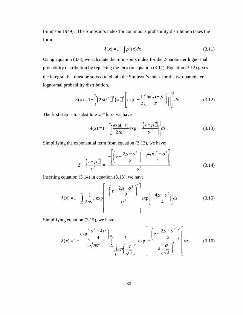
80

(Simpson 1949). The Simpson’s index for continuous probability distribution takes the

form:

2( ) 1 ( )x p x dxλ = − ∫ . (3.11)

Using equation (3.6), we calculate the Simpson’s index for the 2-parameter lognormal

probability distribution by replacing the ( )p x in equation (3.11). Equation (3.12) gives

the integral that must be solved to obtain the Simpson’s index for the two-parameter

lognormal probability distribution.

( ) ( )2

21 22 1 ln( )

( ) 1 2 exp2

xx x dx

θ

µλ πσσ

∞− − − = − −

∫ . (3.12)

The first step is to substitute lnz x= , we have

( )2

2 2

exp( )( ) 1 exp

2

zzx dz

µλ

πσ σ

∞

−∞

−−= − −

∫ . (3.13)

Simplifying the exponential term from equation (3.13), we have:

( )2

2

zZ

µσ−

− − =

22 2 4

2

2 42 4

zµ σ µσ σ

σ

− −− − + . (3.14)

Inserting equation (3.14) in equation (3.13), we have

22

2

2 2

221 4

( ) 1 exp exp2 4

z

x dz

µ σµ σλ

πσ σ

∞

−∞

−− − = − − −

∫ . (3.15)

Simplifying equation (3.15), we have

22 2

22 2

4 2exp

4 21( ) 1 exp

222

22

z

x dz

σ µ µ σ

λσπσ σπ

∞

−∞

− −− = − −

∫ (3.16)

81

The integral part of the above expression is a normal probability density function

with mean 22

2

µ σ− and variance

2

2

σ, and it is equal to 1. The Simpson’s index for the

2-parameter lognormal probability distribution is:

2

2

1 4( ) 1 exp

42x

σ µλπσ

−= −

. (3.17)

Equation (3.17) is also the Simpson’s index for the 3-parameter lognormal probability

distribution. The Shannon-Wiener’s and Simpson’s diversity indices for the two

parameter lognormal probability distribution are given in Table 3.9.

Table 3.9 Shannon-Wiener’s and Simpson’s Diversity Index for the Two-Parameter

Lognormal Probability Distribution.

Diversity Index Two-Parameter Lognormal

Shannon-Wiener 21 1

ln(2 )2 2

πσ µ+ +

Simpson 2

2

1 41 exp

42

σ µπσ

−−

3.5.3 The Diversity Indices for the Probability Distribution of Species Abundance

Knowing the underlying probability distribution of the species abundance data

sets and the corresponding Shannon-Wiener and Simpson’s diversity indices for these

underlying distributions (Table 3.10), we can estimate the indices from the sample of the

population using the underlying probability distribution.

The estimates for the true Shannon-Wiener’s and Simpson’s diversity indices

using the two-parameter lognormal probability distribution for the years from 1996 to

2006 are given in Table 3.9. This table also has the Shannon-Wiener diversity index

obtained in the reports by Yanev et al. (2003a, b, 2004) and Tsokos et al. (2005, 2006a)

obtained using the jackknife procedure and the Shannon-Wiener diversity index without

the jackknife procedure (Direct procedure). The Shannon-Wiener diversity index

82

obtained from the distribution fit approach is much higher than both estimates obtained

through the direct procedure and by using the jackknife procedure. This means that the

estimate under the two-parameter lognormal probability distribution indicates that the

ecosystem is more diverse than the estimates from the other two procedures. We know

that the two estimates obtained from the direct procedure and through the jackknifing

procedure always under represent the true Shannon-Wiener diversity index parameter.

The estimate from the jackknifing procedure is slightly greater than the estimate from the

direct procedure, since it corrects the bias that exists as a result of the sampling

procedure. From the results of the three procedures in obtaining an estimate for the true

Shannon-Wiener, we can say that there are changes in the species distribution over the

years of the CREMP. In Table 3.10, there are two time periods: from 1996 to 1999 and

from 2000 to 2006 that show different patterns of the Shannon-Wiener diversity index

estimates. The values from 1996 to 1999 are higher than the values from 2000 to 2006.

This means that the ecosystem in the sanctuary had more uncertainty of knowing which

species an individual belongs too prior to 1999 as compared to post 1999.

Table 3.10 Shannon-Wiener’s and Simpson’s Diversity Index for The Species

Abundance Data.

Shannon-Wiener Simpson Year Distribution Jackknife Original Distribution 1996 6.62 2.31 2.29 0.9933 1997 6.64 2.30 2.27 0.9944 1998 6.33 2.19 2.16 0.9918 1999 6.26 1.97 1.95 0.9936 2000 5.91 2.06 2.04 0.9882 2001 6.13 2.04 2.02 0.9910 2002 6.18 2.16 2.14 0.9920 2003 6.12 2.08 2.07 0.9908 2004 6.21 2.10 2.08 0.9920 2005 6.12 2.08 2.07 0.9911 2006 5.97 2.00 1.98 0.9886

The Simpson’s diversity index estimates from 1996 to 2006, Table 3.10, are close

to each other. These values indicate that there is a high probability that two individuals

83

in the sanctuary region, through the sample, belong to different species. We can interpret

this as meaning that the ecosystem is very diverse.

The percentage improvement of the estimates of the true Shannon-Wiener

diversity index using the underlying probability distribution of the species abundance

data as compared to the other two procedures are given in Table 3.11. The percentage

improvement is very encouraging that we can estimate the true Shannon-Wiener diversity

index from a sample of the population.

Table 3.11 Percentage Differences of the Shannon-Wiener Diversity Index: PDF vs.

Jackknifing Procedure and Direct Procedure.

Percentage Change Year Jackknife Original 1996 186 190 1997 189 192 1998 189 192 1999 218 221 2000 186 190 2001 201 204 2002 186 189 2003 194 196 2004 196 199 2005 194 196 2006 199 202

Figure 3.3 shows the differences between the Shannon-Wiener diversity indices

using the three approaches. The estimates from the two-parameter lognormal probability

distribution are much larger than from the other two procedures. It can be seen that all

three seem to follow the same pattern through the years. Thus, the results of this study

should be used to understand and monitor the diversity of the stony coral as required by

CREMP.

84

Figure 3.3 Shannon-Wiener Diversity Indices for the Sanctuary Region. DSV = Index from the PDF JSV = Index from the Jackknife

Procedure OSV = Index directly from the Sample

0

1

2

3

4

5

6

7

1994 1996 1998 2000 2002 2004 2006

Year

Sha

nnon

Inde

x

DSV

JSV

OSV

85

3.6 Conclusion

In investigating the normality assumption of the pseudovalues of the jackknife

procedure for the Shannon-Wiener diversity index estimate, we found that the Dry

Tortugas with only 12 pseudovalues tested positive for normality through the Shapiro-

Wilks normality test. While this is true of the pseudovalues for the Dry Tortugas for each

year (1999 to 2006), the same cannot be said for the 105 pseudovalues from the sanctuary

region for each year from 1996 to 2006. The sanctuary pseudovalues failed to support

the null hypothesis that the data came from a normal distribution under the Shapiro-Wilks

normality test. Also the bootstrap empirical confidence intervals for the pseudovalues

from the jackknife procedure are shorter than the ones obtained using the normality

assumption. This was true for the sample sizes of 12 and 105 using the two sets of

bootstrap repetitions 100, 200 and 500, and 1500, 5000 and 10000. The difference in

confidence range was greater for the 12 pseudovalue samples than for the 105 samples. In

the case of the sample size of 12, the bootstrap empirical confidence interval was always

contained inside the confidence interval with the normality assumption. Although this

was not the case with the sample size of 105, the bootstrap empirical confidence intervals

were lower than the confidence intervals under the normality assumption but they had

very close values for both upper and lower confidence bounds. The jackknife procedure

is still essential in the study of diversity indices due to its biased reduction capability and

the advantages of having the pseudovalues. The advantages of the jackknife procedure

can be enhanced with the use of bootstrapping in creating the confidence interval of the

Jackknife estimates.

The results of the Shapiro-Wilks normality test show that the normality

assumption plays no role in the difference found between the confidence intervals for the

jackknife estimate from the normality assumption on the pseudovalues and from the

bootstrap procedure. This statement can be defended using two angles of analytical

reasoning. First we looked at the approach of using the normality statistical testing of the

samples. The pseudovalues from Dry Tortugas tested positive for normality and the

pseudovalues from the sanctuary did not. Yet the confidence intervals from both

86

approaches for the non-normal distributed samples (sanctuary) were much closer than for

the normally distributed samples (Dry Tortugas). The second point of view is that one

can assume normality for the large sample through the central limit theorem. This again

leads to the same conclusion that the difference in confidence interval is not due to the

normality assumption. In this case this is true, since both samples would be normally

distributed but still have differences in the confidence intervals. It is quite possible that

the difference is due to the sample size but this has to be further investigated.

With respect to investigating the diversity index through the probability

distribution fit of the sanctuary species abundance data, the two-parameter lognormal was

a very good fit to the species abundance for all the years. We can therefore use

parametric analysis to improve the results from the works of Yanev et al. (2003a, b,

2004) and Tsokos et al. (2005, 2006a) for the CREMP. From the probability distribution,

we calculated the estimate of the true Shannon-Wiener diversity indices. These are much

higher than the ones obtained from the jackknife procedure or from the direct method. By

finding the probability distribution of the species abundance, more weight was given to

the rare or less abundant species, while still considering the contribution of the most

abundance species to the habitat. The high values are also a result of the attempt to

account for species not represented or recorded due to sampling. The high values of the

Shannon-Wiener indicate high diversity among the stony coral species within the

sanctuary. There is an indication that a decrease in diversity occurred between 1996 and

2006 in the sanctuary region.

We were able to solve the Simpson’s diversity index for the two-parameter

lognormal probability. This is important as it provides scientists, who prefer to use the

Simpson’s diversity index, another better approach of estimating the true Simpson’s

diversity index.

We can now use the results here to improve the previously obtained results from

the works of Yanev et al. (2003a, b, 2004) and Tsokos et al. (2005, 2006a). More

importantly the results can be used in general to effectively examine stony coral species

data that contain the different types of species and their abundances.

87

Chapter 4

Nonparametric Statistical Analysis of Diversity Index

4.1 Introduction

The focus of Chapter 3 was to investigate the normal probability distribution

assumption made on the pseudovalues obtained from the jackknife procedure for the

Shannon-Wiener diversity index used in the works of Yanev et al. (2003a, b, 2004) and

Tsokos et al. (2005, 2006a) for the CREMP. The Dry Tortugas pseudovalues showed

statistical evidence that they are normally distributed but this was not so for the sanctuary

pseudovalues. The normality assumption was used in the construction of the 95%

confidence interval for the Shannon-Wiener diversity indices for the entire sanctuary for

years from 1996 to 2005. Since the underlying assumption of normality was used to

obtain the confidence intervals using the pseudovalues, they cannot be used for decision

making. Such a decision would be misleading. We tried to fit other continuous

probability distributions so that we can proceed with parametric analysis without any

success. Thus, we will proceed nonparametrically by estimating the probability

distribution function using the kernel density approach. This nonparametric procedure

has been applied successfully (e.g. Baxter, Beardah and Wright 1997, Ker and Goodwin

2000, Wolf and Sumner 2001, Lotti and Santarelli 2004, Buskirk and Lohr 2005) in

estimating the probability distribution function when a classical well defined probability

distribution function could not be found to fit the data. Hence, the aim of this chapter is

to develop the best possible estimate of the probability distribution of the jackknifing

pseudovalues for the sanctuary using the kernel density method. Once the best kernel

density estimate is obtained, a comparison with the parametric approach under the normal

88

assumption will be made. We compare the mean, standard deviation, standard error and

the 95% confidence interval of the true mean.

4.2 Kernel Probability Density

Many scientists have studied the development of nonparametric density

estimation methods using kernels and bandwidths. For example Tapia and Thompson

(1978), Bean and Tsokos (1980), Silverman (1986), and Liu (1998) have found

interesting analytical results and documented the importance of nonparametric density

estimation methods to various applications. Silverman (1986), Liu (1998), and Liu and

Tsokos (2002), among others, have shown that once a good bandwidth estimate has been

identified the kernel density estimation is very accurate and effective. Liu (1998) and Liu

and Tsokos. (2002) showed that the optimal bandwidth is different for both the kernel

probability distribution function and kernel cumulative distribution function. Tapia and

Thompson (1978), Silverman (1986), Liu (1998), and Liu and Tsokos (2002), all stress

that the bandwidth is much more important than the choice of the kernel used. Silverman

(1986) suggested that the choice of kernel be considered on the degree of differentiability

required or the computation effort involved.

Let 1,..., nX X be a sample of independent, identically distributed observations

having a common pdf, ( )f x , then ˆ ( )f x will denote the kernel density estimate to ( )f x .

ˆ ( )f x is defined by

1

1ˆ( )n

i

i

x Xf x K

nh h=

− =

∑ (4.1)

where K is the kernel function, n is the sample size and h is the bandwidth. From

equation (4.1), both the kernel function and bandwidth are needed to obtain the kernel

density estimate of ( )f x . It is also assumed that the underlying probability density

function ( )f x has continuous derivatives of all orders.

89

First, we shall summarize some of the basic properties of ˆ ( )f x . The kernel

function K is usually restricted to be a symmetric probability density function. It means

that the kernel function satisfies the following conditions:

( ) 1K t dt∞

−∞=∫ , ( ) 0tK t dt

∞

−∞=∫ , and 2

2( ) 0t K t dt k∞

−∞= ≠∫

Properties of K define the properties of the resulting kernel estimate ˆ( )f x . Since K is a

probability density function, then ( )f x is also a probability density function. Table 4.1

gives a list of commonly used kernel functions. From the commonly used kernel

function, all except the Gaussian kernel function have a bounded sample space.

Table 4.1 Some Kernels and Their Inefficiencies.

Kernel ( )K t Inefficiency Epanechnikov 23 1

154 5

t −

for 5t < 1

Biweight ( )22151

16t− for 1t <

1.0061

Triangular 1 t− for 1t < 1.0143

Gaussian 2

21

2

t

eπ

−

1.0513

Uniform 1

2 for 1t <

1.0758

From the kernel density estimate, equation (4.1), the bandwidth (h) controls how

many observations appear around x in the kernel density estimate. If h is too small, too

few observations around x are considered in the stability of the kernel density estimate.

The kernel density estimate produces too many bumps. On the other hand, if the

bandwidth is too large, many observations around x are considered in the stability of the

kernel density estimate, causing over smoothness of the kernel density estimate.

The inefficiency of the kernel function gives an indication of its performance on

the kernel density estimate based on the criteria of the mean integrated square error

(MISE). The Epanechnikov kernel function is the most efficient under the MISE criteria

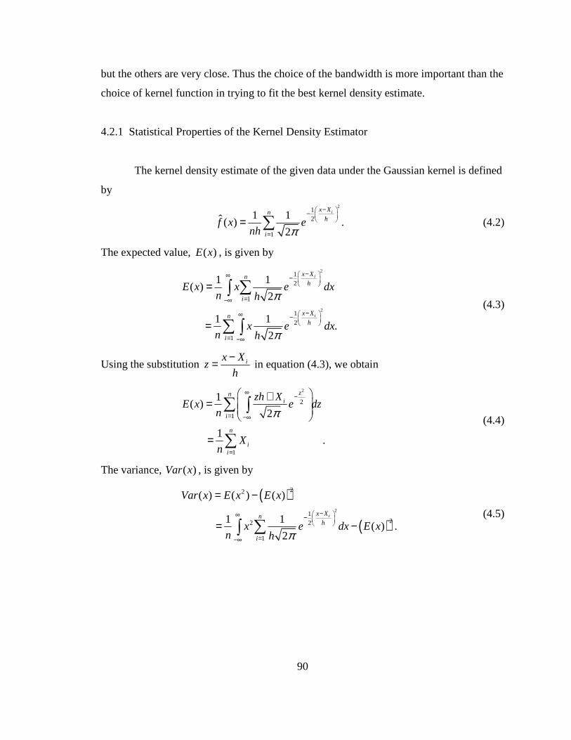
90

but the others are very close. Thus the choice of the bandwidth is more important than the

choice of kernel function in trying to fit the best kernel density estimate.

4.2.1 Statistical Properties of the Kernel Density Estimator

The kernel density estimate of the given data under the Gaussian kernel is defined

by 2

12

1

1 1ˆ( ) .2

ix Xnh

i

f x enh π

− −

=

= ∑ (4.2)

The expected value, ( )E x , is given by

2

2

12

1

1

2

1

1 1( )

2

1 1.

2

i

i

x Xnh

i

x Xnh

i

E x x e dxn h

x e dxn h

π

π

− ∞ −

=−∞

− ∞ −

= −∞

=

=

∑∫

∑ ∫

(4.3)

Using the substitution ix Xz

h

−= in equation (4.3), we obtain

2

2

1

1

1( )

2

1.

zni

i

n

ii

zh XE x e dz

n

Xn

π

∞−

= −∞

=

+=

=

∑ ∫

∑

(4.4)

The variance, ( )Var x , is given by

( )

( )2

22

122 2

1

( ) ( ) ( )

1 1( ) .

2

ix Xnh

i

Var x E x E x

x e dx E xn h π

− ∞ −

=−∞

= −

= −∑∫ (4.5)

91

We can show the results for 2( )E x to be

( )

2

2

12 2 2

1

22

1

2 2

1

1 1( )

2

( )1

2

1.

ix Xnh

i

zni

i

n

ii

E x x e dxn h

zh Xe dz

n

h Xn

π

π

− ∞ −

= −∞

∞−

= −∞

=

=

+=

= +

∑ ∫

∑ ∫

∑

(4.6)

By combining equations (4.4) and (4.6), the variance is given as:

( )

( )

22

2

2 2

1 1

22

1

( ) ( ) ( )

1 1

1.

n n

i ii i

n

ii

Var x E x E x

h X Xn n

h X Xn

= =

=

= −

= + −

= + −

∑ ∑

∑

(4.7)

To obtain the interval that contains 95% of the true mean using the kernel density

estimate, we will calculate the cumulative distribution function (cdf) of the kernel density

estimate. The cdf is defined by 2

2

1

2

1

2

1

1

1 1ˆ ( )2

1 1

2

1.

i

i

t Xxnh

i

x Xzhn

i

ni

i

F x e dtn h

e dzn

x X

n h

π

π

− −

= −∞

−

−

= −∞

=

=

=

− = Φ

∑ ∫

∑ ∫

∑

(4.8)

From the cdf in equation (4.8), we can now formulate the 95% confidence interval of the

true mean of the unknown underlying probability distribution for the jackknifing

92

pseudovalues from the sanctuary. Table 4.2 gives a summary of the results for the

expected value, variance and the cumulative density function.

Table 4.2 Expected Value, Variance and Cumulative Distribution Function of the Kernel

Density Estimate.

Gaussian Kernel Density Estimate

Expected Value

1

1 n

ii

Xn =∑

Variance ( )22

1

1 n

ii

h X Xn =

+ −∑

CDF

1

1 ni

i

x X

n h=

− Φ

∑

4.2.2 Criteria for Quality of Fit

Here we identify the criteria that we use to evaluate the quality of ( )f x . We

employ the mean integrated square error (MISE) which was developed from the mean

square error (MSE) which is a measurement of error at single points. MSE is defined by

( )2ˆ ( ) ( )MSE E f x f x= − . (4.9)

Expanding equation (4.9) we have

( )2ˆ ˆ( ) ( ) var ( )MSE Ef x f x f x= − + .

This expression shows that MSE has two components, the sum of squared bias and the

variance. Rosenblatt (1956) introduced the concept of MISE which allows obtaining a

better approximation of the MSE measurement. The MISE is defined by

( )( )

2

2

ˆ ( ) ( )

ˆ ˆ( ) ( ) var ( ) .

MISE E f x f x dx

Ef x f x dx f x dx

= −

= − +

∫

∫ ∫ (4.10)

The approximations for theses two integrals can be found in Silverman (1986).

93

It allows for the estimations of the bias portion of the MISE to be obtained from

( )ˆ ( ) ( )

( ) /( ) ( )

bias Ef x f x

K x y hf y dy f x

h

= −−

= −∫ (4.11)

By using the substitution y x ht= − and a Taylor series expansion of equation (4.11), the

following approximation to the bias portion of the MISE is obtained.

2 2 21( ) ( ) ( )

2bias h f x t K t dt o h′′= +∫ . (4.12)

The integral of the square of equation (4.12) is then taken to complete the first part of

equation (4.10). That is,

42 2 2( ) ( )

4

hbias dx t K t dt f x dx′′≈∫ ∫ ∫ . (4.13)

The integral of the variance is found similarly giving the following approximation:

21ˆvar ( ) ( )f x dx K t dtnh

≈∫ ∫ . (4.14)

The importance of the results of equation (4.13) and (4.14) is that MISE depends

on the choice of h andK . Since the efficiency of theK ’s are very similar, the selection

of the choice of h becomes very important. The value of h can’t be too small or too

large. A large value will increase the bias and a small value would increase the variance.

We selected to work with the Gaussian kernel for two reasons: the Gaussian is

differentiable everywhere and xcan exist everywhere (not limited to a certain range).

Even though we selected to work with the Gaussian kernel, we tried the other commonly

used kernel functiosn such as Epanechnikov, rectangular, triangular, etc. and concluded

that the Gaussian gave a better approximation. The major problem was obtaining the best

bandwidth (h ). Silverman (1986) suggested a few rules of thumb for bandwidths when

using the Gaussian kernel. The rule of thumb bandwidths are given below:

1/51

1/52

1/53

ˆˆ ˆ1.06min( , )1.34ˆ ˆ0.79

ˆˆ ˆ0.9min( , ) .1.34

Rh n

h Rn

and

Rh n

σ

σ

−

−

−

=

=

=

(4.15)

94

where σ is the estimate of the standard deviation and R is an estimate of the inter-

quartile range of the sample. Silverman (1986) also investigated the results of these three

bandwidth. He suggests using 2h and 3h whenever the data sets are skewed. But we

encounter problems with 2h whenever a bimodal behavior appears in the data. In such

case, he suggests to use either 1h or 3h . A good approximation of MISE, is given below,

when using the Gaussian kernel:

2 2 2 2

2 2

1 1 1 1 12

2 2 .2

MISE n h h h

h

π σσ σ

σ

= − + + + +

−+

(4.16)

Using this approximation of MISE we obtain good results.

4.3 Procedure for Developing the Kernel Density Estimate

We will fit the kernel density estimate for all the jackknife pseudovalues samples

from 1996 to 2006. It is important that the observations in each sample are independent.

Zahl (1977) showed that these values can be considered to be independent.

The histogram will be used in the fitting process, it is necessary to standardize the

plotting procedure of the histogram. The bin size of all the histogram will be 1 and the

first break occurred at smallest integer in the data set. The bandwidth will be chosen by

using the rule of thumb formulas in equation (4.15) and the MISE, equation (4.16). We

used the rule of thumb values as a starting point, increasing its value by 0.05 until a

suitable fit is seen along with a small MISE value. This will be considered the best

kernel estimate for the unknown underlying probability distribution of the sample.

4.4 The Kernel Density Estimate

We fitted the kernel density estimate using the Gaussian kernel to the jackknifing

pseudovalues for the stations in the sanctuary. We found the maximum likelihood

95

estimates for the parameters of the normal probability distribution that is assumed under

the jackknifing procedure.

Table 4.3 has the bandwidth and MISE for each of the kernel density estimates to

the underlying probability density distribution for the years 1996 to 2006. The

bandwidths for all the years were found to be around 0.3 to 0.5. As the results show the

MISE values are all very small, less than 0.006.

Table 4.3 Parameter Estimates for the Kernel Density Estimate and the Normal

Probability Distribution.

Kernel Density Normal Distribution Year Bandwidth MISE Mean Std Dev 1996 0.350 0.0058 2.31 1.03 1997 0.364 0.0056 2.30 1.06 1998 0.332 0.0061 2.19 1.10 1999 0.495 0.0049 1.97 1.07 2000 0.419 0.0054 2.06 0.98 2001 0.366 0.0056 2.04 1.07 2002 0.362 0.0057 2.16 1.00 2003 0.329 0.0062 2.08 1.15 2004 0.333 0.0061 2.10 1.18 2005 0.390 0.0053 2.08 1.08 2006 0.460 0.0050 2.00 1.06

One criterion in selecting the bandwidth is to use the bandwidth with the

minimum MISE. In 1996, as shown in Figure 4.1, there exists a bandwidth with a

minimum MISE. This MISE occurs at a bandwidth of 0.452 with a MISE value of

0.0051. The bandwidth chosen was 0.35 with a MISE value of 0.0058 which is close to

the lowest MISE value possible. We chose to use the bandwidth 0.350 rather than 0.452,

since it gave a better fit to the histogram, (Figure 4.2).

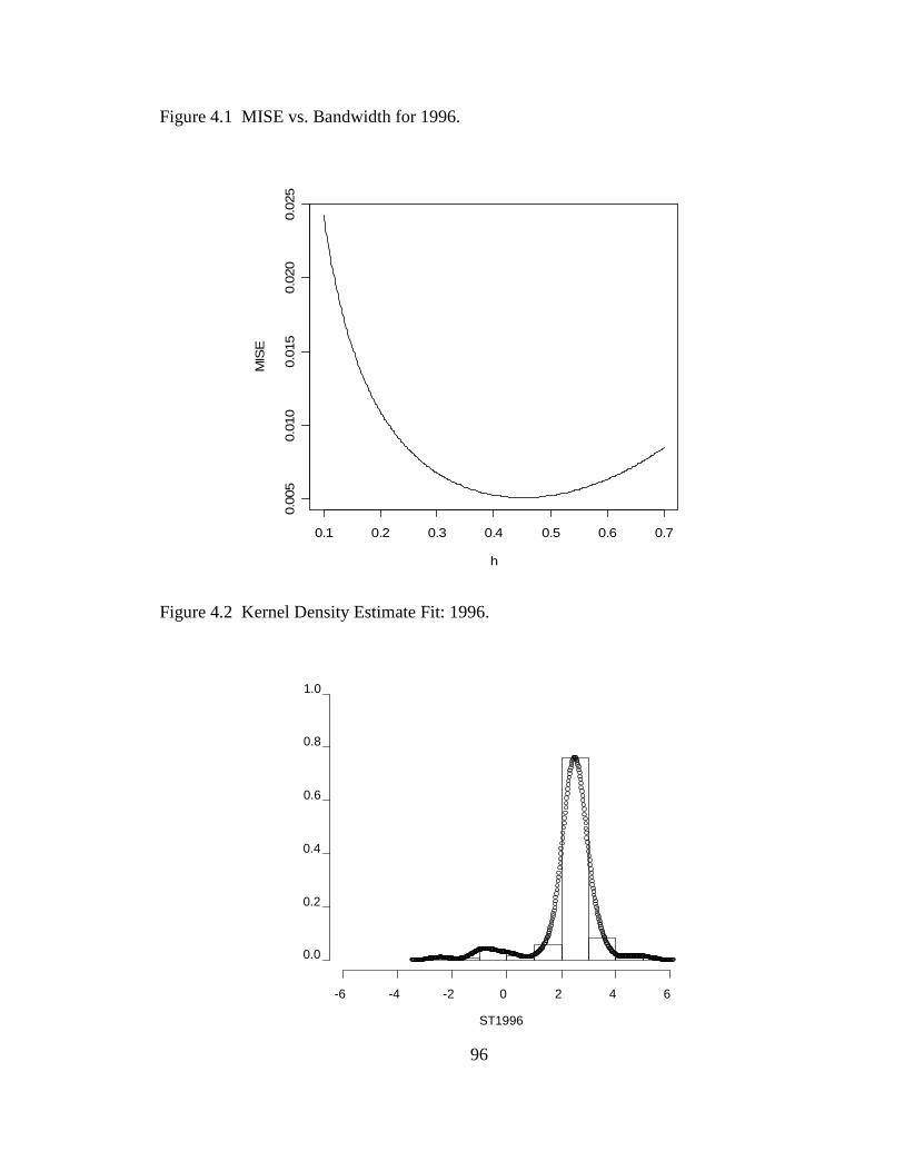
96

Figure 4.1 MISE vs. Bandwidth for 1996.

0.1 0.2 0.3 0.4 0.5 0.6 0.7

0.00

50.

010

0.01

50.

020

0.02

5

h

MIS

E

Figure 4.2 Kernel Density Estimate Fit: 1996.

ST1996

-6 -4 -2 0 2 4 6

0.0

0.2

0.4

0.6

0.8

1.0

97

Table 4.1 also shows the MLE for both parameters of the normal distribution fit

for the same jackknifing pseudo values. Here we must reiterate, that the goodness-of-fit

statistics used in Chapter two all showed that the normal probability distribution is not a

good fit to the jackknifing pseudovalues. Figure 4.3 show the normal probability

distribution fit to the jackknifing pseudovalues to the data. We can see from Figures 4.2

and 4.3 that the Gaussian kernel density estimate fits the data very well and is better than

the normality probability distribution fit. We tried to fit other continuous probability

distribution functions to the data such as the lognormal, Weibull, gamma and others with

no success.

Figure 4.3 Normal Distribution Fit: 1996.

The main problem with the data values is the high peaks that occur, giving the

existing probability distribution trouble to fit but does not pose a problem for the kernel

density estimate. Similarly, close fit results as seen for 1996 is seen for the data of the

other nine years. The kernel density estimate versus the normality probability

ST1996

-6 -4 -2 0 2 4 6

0.0

0.2

0.4

0.6

0.8

1.0

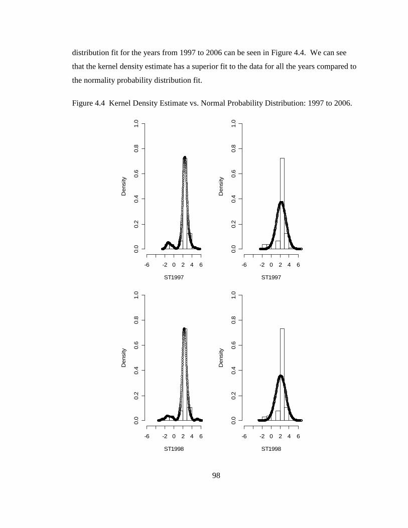
98

distribution fit for the years from 1997 to 2006 can be seen in Figure 4.4. We can see

that the kernel density estimate has a superior fit to the data for all the years compared to

the normality probability distribution fit.

Figure 4.4 Kernel Density Estimate vs. Normal Probability Distribution: 1997 to 2006.

ST1997

Den

sity

-6 -2 0 2 4 6

0.0

0.2

0.4

0.6

0.8

1.0

ST1997

Den

sity

-6 -2 0 2 4 6

0.0

0.2

0.4

0.6

0.8

1.0

ST1998

Den

sity

-6 -2 0 2 4 6

0.0

0.2

0.4

0.6

0.8

1.0

ST1998

Den

sity

-6 -2 0 2 4 6

0.0

0.2

0.4

0.6

0.8

1.0

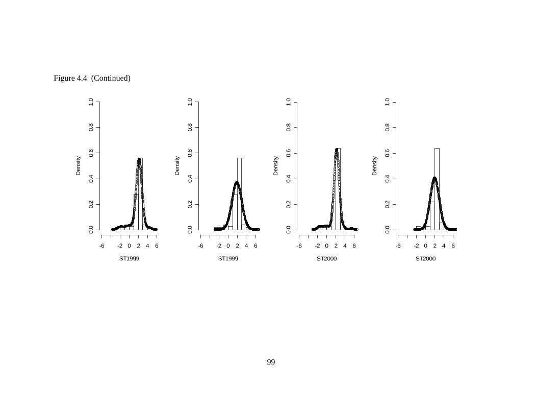
99

Figure 4.4 (Continued)

ST1999

Den

sity

-6 -2 0 2 4 6

0.0

0.2

0.4

0.6

0.8

1.0

ST1999

Den

sity

-6 -2 0 2 4 6

0.0

0.2

0.4

0.6

0.8

1.0

ST2000

Den

sity

-6 -2 0 2 4 6

0.0

0.2

0.4

0.6

0.8

1.0

ST2000

Den

sity

-6 -2 0 2 4 6

0.0

0.2

0.4

0.6

0.8

1.0

100

Figure 4.4 (Continued)

ST2001

Den

sity

-6 -2 0 2 4 6

0.0

0.2

0.4

0.6

0.8

1.0

ST2001

Den

sity

-6 -2 0 2 4 6

0.0

0.2

0.4

0.6

0.8

1.0

ST2002

Den

sity

-6 -2 0 2 4 6

0.0

0.2

0.4

0.6

0.8

1.0

ST2002

Den

sity

-6 -2 0 2 4 6

0.0

0.2

0.4

0.6

0.8

1.0

101

Figure 4.4 (Continued)

ST2003

Den

sity

-6 -2 0 2 4 6

0.0

0.2

0.4

0.6

0.8

1.0

ST2003

Den

sity

-6 -2 0 2 4 6

0.0

0.2

0.4

0.6

0.8

1.0

ST2004

Den

sity

-6 -2 0 2 4 6

0.0

0.2

0.4

0.6

0.8

1.0

ST2004

Den

sity

-6 -2 0 2 4 6

0.0

0.2

0.4

0.6

0.8

1.0

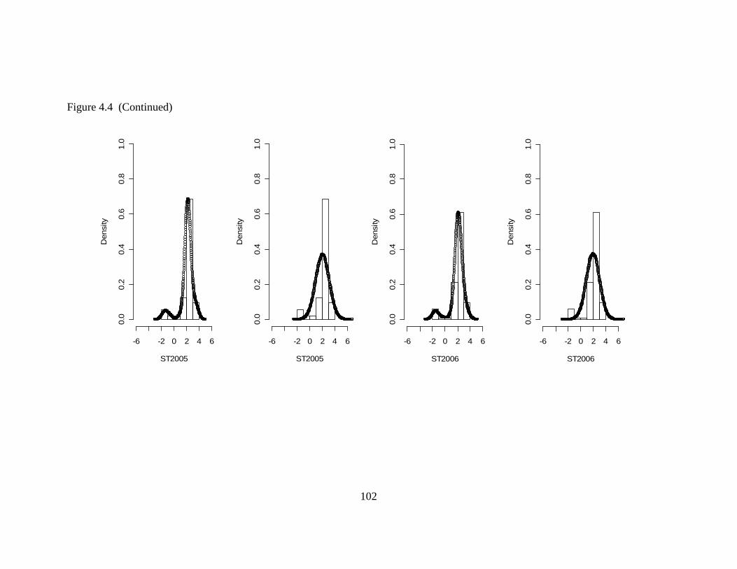
102

Figure 4.4 (Continued)

ST2005

Den

sity

-6 -2 0 2 4 6

0.0

0.2

0.4

0.6

0.8

1.0

ST2005

Den

sity

-6 -2 0 2 4 6

0.0

0.2

0.4

0.6

0.8

1.0

ST2006

Den

sity

-6 -2 0 2 4 6

0.0

0.2

0.4

0.6

0.8

1.0

ST2006

Den

sity

-6 -2 0 2 4 6

0.0

0.2

0.4

0.6

0.8

1.0

103

The Gaussian kernel density estimate for 1996 pseudovalues data is given by

2

11052 0.35

1

1 1ˆ( ) .36.75 2

ix X

i

f x eπ

− −

=

= ∑ (4.17)

Similar Gaussian kernel density estimate can be written for the pseudovalues data for the

other years using the estimates in Table 4.3 and equation (4.2).

4.5 Comparison of the Nonparametric and Parametric

Although using the normal probability distribution is not valid and is not

recommended to be used, we proceed to compare the results with the kernel density

estimate of the pseudovalues data.

Table 4.4-A and Table 4.4-B gives the mean, standard deviation, standard error,

and the 95% confidence interval of the true mean from the Gaussian kernel density

estimate and from the normal probability distribution, respectively.

Table 4.4-A Statistical Properties of the Gaussian Kernel Density Estimate.

95% Year Mean Std Dev Std Error Upper Lower 1996 2.31 1.08 0.105 3.858 -0.969 1997 2.30 1.11 0.109 3.908 -1.271 1998 2.19 1.15 0.112 3.730 -1.494 1999 1.97 1.18 0.115 3.814 -1.625 2000 2.06 1.06 0.103 3.651 -1.170 2001 2.04 1.13 0.110 3.448 -1.859 2002 2.16 1.06 0.103 3.966 -1.204 2003 2.08 1.19 0.117 3.694 -1.937 2004 2.10 1.22 0.119 3.681 -2.028 2005 2.08 1.14 0.111 3.795 -1.501 2006 2.00 1.15 0.113 3.675 -1.617

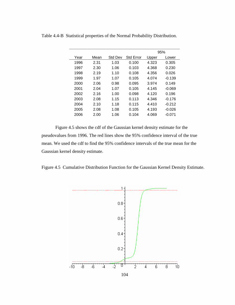
104

Table 4.4-B Statistical properties of the Normal Probability Distribution.

95% Year Mean Std Dev Std Error Upper Lower 1996 2.31 1.03 0.100 4.323 0.305 1997 2.30 1.06 0.103 4.368 0.230 1998 2.19 1.10 0.108 4.356 0.026 1999 1.97 1.07 0.105 4.074 -0.139 2000 2.06 0.98 0.095 3.974 0.149 2001 2.04 1.07 0.105 4.145 -0.069 2002 2.16 1.00 0.098 4.120 0.196 2003 2.08 1.15 0.113 4.346 -0.176 2004 2.10 1.18 0.115 4.410 -0.212 2005 2.08 1.08 0.105 4.193 -0.026 2006 2.00 1.06 0.104 4.069 -0.071

Figure 4.5 shows the cdf of the Gaussian kernel density estimate for the

pseudovalues from 1996. The red lines show the 95% confidence interval of the true

mean. We used the cdf to find the 95% confidence intervals of the true mean for the

Gaussian kernel density estimate.

Figure 4.5 Cumulative Distribution Function for the Gaussian Kernel Density Estimate.

105

The estimates for the true expected mean are equal for both the Gaussian kernel

density estimate and the normal probability distribution, Tables 4.4-A and 4.4-B.

The standard error is a monotone function of the standard deviation, comparing

one of these is sufficient in comparing the other. We compare the standard deviations.

Figure 4.6 shows a graph of the standard deviation for both probability distribution

functions. The standard deviation for the Gaussian kernel density estimate is larger than

that for the normal distribution for every year.

Figure 4.6 Standard Deviations: Gaussian Kernel Density Estimate (KDE) vs. Normal

Probability Distribution (N).

0.70

0.80

0.90

1.00

1.10

1.20

1.30

1.40

1.50

1994 1996 1998 2000 2002 2004 2006 2008

KDE

N

The results from the 95% confidence intervals for the true mean is important as

shown in the works by Yanev et al. (2003a, b, 2004) and Tsokos et al. (2005, 2006a) for

the CREMP. In those works, the confidence intervals for the true mean of the

pseudovalues data sets were constructed under the normality assumption. This mean

value is the estimate for the true Shannon-Wiener diversity index of the stony corals. The

results of the confidence interval are given in Tables 4.4-A and 4.4-B. In Figure 4.7, the

106

blue solid line is the interval for the normal distribution and the red dotted line represents

the interval from the kernel density estimator. The 95% confidence intervals are

completely different using the Gaussian kernel density estimate and the normal

probability distribution.

Figure 4.7 95 % Confidence Interval: Gaussian Kernel Density Estimate (KDE) vs.

Normal Probability Distribution (N).

-3

-1

1

3

5

1994 1996 1998 2000 2002 2004 2006 2008

KDE

N

4.6 Conclusion

We have shown that the Gaussian kernel density estimate is clearly a much better

fit to the jackknifing pseudovalues compared to the normal probability distribution and

other continuous probability distributions. A good estimate of the true probability

structure of the pseudovalues data is imperative for sound decision making. The estimates

of the statistical properties of the data obtained from the Gaussian kernel density estimate

are different than the ones from the normal probability distribution.

107

The results presented in this chapter can help analyze and interpret the Shannon-

Weiner diversity index of the stony coral for the CREMP. A better understanding of the

underlying probability distribution of the jackknifing pseudovalues can enhance the

advantages of using the jackknifing method in obtaining a good estimate of the Shannon-

Wiener diversity index and providing data that can be used in the statistical analysis and

interpretation of the Shannon-Wiener diversity index. Furthermore, we have shown that

one cannot just assume that the pseudovalues obtained from the jackknifing procedure are

normally distributed as suggested by Zahl (1977). This assumption can lead to obtaining

false information.

108

Chapter 5

Statistical Modeling of Stony Coral Cover

5.1 Introduction

The coral reef communities are very important ecosystems in the world. They are

home to at least 4,000 species and almost a third of the world’s marine fish species

(Paulay 1996). Coral reefs have ecological and economic significance throughout the

world. Ecologically for Florida and elsewhere, they provide habitat for fish and

macroinvertebrates. They also serve as protection against wave action, especially during

storm surges and they provide source of coral rubble and sand. Coral reefs can also be the

base for island formation, as well as maintaining and replenishing beaches. The economic

significance for Florida’s coral reefs is enormous, especially for the tourist industry and

the generation of marine products for commercial export. Tourism generates over $50

billion a year; in 2003 over 74 million visitors engaged in reef-based activities in Florida

(Andrews et al. 2005).

Coral reefs are very specialized communities that are highly sensitive to local,

regional, and global environmental changes; therefore it is very important to learn as

much as we can about this system. As Hallock (1997) warned, the recovery of reef

building communities from extinction events requires millions of years. With this in

mind, we believe a statistical model to predict an estimate stony coral cover proportion

would be very beneficial to monitor ecosystem health of coral reefs. This would give

scientists another tool to understand what environmental factors drive the coral reef

ecosystem. Since reefs are complex systems, it is virtually impossible to represent all

interactions in one statistical model of the ecosystem with a few parameters.

109

Nevertheless, it is imperative to try to model the information that is available to us.

Having such a statistical model will assist the managers in making decisions that would

be meaningful for ecosystem conservation.

The focus of this chapter is to develop a statistical predictive model of stony coral

cover proportion. Such a model would identify the attributable variables that influence

the stony coral cover. The quality of the model will be a function of the limited data that

are available on the subject matter.

5.2 Response and Attributable Variables

The response variable is the stony coral cover proportion data obtained from

CREMP, which is one of the components of the Water Quality Protection Program

(WQPP) instituted for the Florida Keys National Marine Sanctuary (FKNMS).

The attributable variables were obtained from the both the CREMP and the Water

Quality Monitoring Project (WQMP). WQMP is the other component of the WQPP

instituted for the Florida Keys National Marine Sanctuary by EPA in 1995. Data were

provided by the Southeast Environmental Research Center-Florida International

University, Water Quality Monitoring Network which is supported by SFWMD/SERC

Cooperative Agreements #C-10244 and #C-13178 as well as EPA Agreement #X994621-

94-0. Sampling is done on a quarterly basis for more than 200 stations in the FKNMS and

Shelf since March 1995 by SERC (Boyer and Jones 2002).

The attributable variables obtained from CREMP are station location: latitude and

longitude, depth of the station: inshore and offshore and type of stony coral reef: patch,

shallow, hardbottom and deep. The attributable variables obtained from WQMP project

are total nitrogen, total phosphorus, chlorophyll a, total organic carbon, turbidity, salinity

and temperature. Both surface and bottom measurements were considered. These

attributable variables were chosen from among other variables collected by WQMP

project on the advice of Walter Jaap, a leading scientist in the field of corals and who has

worked many years with Florida Fish and Wildlife Research Institute (FWRI and

CREMP until he retired). He suggested these as strong contributing variables that will

110

influence stony coral cover. Table 5.1 gives the mathematical notations of the variables

used in the present study.

Table 5.1 Notation of Variables.

Notation Variable CC Coral Cover T Arcsine transformation of coral cover lat Latitude of the CREMP station lon Longitude of the CREMP station INSD Inshore Depth of the CREMP station OSD Offshore Depth of the CREMP station P1 Patch reef S1 Shallow reef D1 Deep reef TN Total nitrogen TP Total phosporus CHLA Chlorophyll a TOC Total organic carbon TURB Turbidity SAL Salinity TEMP Temperature

5.3 Data Manipulation

The first major problem that we encountered was that the sister projects (CREMP

and WQMP) do not sample at the exact stations. The matching of the stations from both

projects were obtained from Callahan (2005). He used an Arcview query tool developed

by FWRI to create such matching. Water-quality stations were chosen based on four main

criteria: 1) proximity to CREMP sites, 2) depth similarity, 3) relative distance to shore,

and 4) similarity of benthic cover under the WQMN station (i.e., reef/ hardbottom/

seagrass). Due to the close proximity of some of the CREMP, deep and shallow reef

stations, both stations were paired with the same water-quality station. This allowed us to

obtain data for only 27 stations for which data was collected within the sanctuary region

of the CREMP. The matching stations are given in Table 5.2.

111

Table 5.2 CREMP and WQMP Stations Pairing List.

CREMP Stations WQMP Stations 9P1 Turtle Patch 212 Turtle Harbor 9S1 Carysfort Shallow 216 Carysfort Reef 9D1 Carysfort Deep 216 Carysfort Reef 9S2 Grecian Rocks 400 Grecian Rocks 9P3 Porter Patch 400 Grecian Rocks 9H2 El Radabob 220 Radabob Key 9S3 Molasses Shallow 225 Molasses Reef 9P4 Admiral Patch 224 Molasses Reef Channel 9S4 Conch Shallow 228 Conch Reef 9D4 Conch Deep 264 Aquarius 7S1 Alligator Shallow 401 Alligator Reef 7S2 Tennessee Shallow 243 Tennessee Reef 7D2 Tennessee Deep 243 Tennessee Reef 7H2 Long Key 242 Long Key Channel 7P1 West Turtle 248 Coffins Patch Channel 7P2 Dustan Rocks 248 Coffins Patch Channel 5S1 Sombrero Shallow 402 Sombrero Key 5S2 Looe Key Shallow 263 Looe Key 5D2 Looe Key Deep 263 Looe Key 5P4 Jaap Reef 268 Saddlebunch Keys 5P1 W. Washer Woman 269 W. Washerwoman 5S3 Eastern Sambo Shallow 273 Eastern Sambo Offshore 5D3 Eastern Sambo Deep 273 Eastern Sambo Offshore 5S4 Western Sambo Shallow 403 Western Sambo 5D4 Western Sambo Deep 403 Western Sambo 2D1 Sand Key Deep 281 Middle Ground 3H1 Content Keys 302 Content Passage

The second problem was one of missing values in some of the environmental

variables: TN, TP, TURB and TOC for stations of the WQMP numbered: 216, 224, 268

and 302. The second quarter sampling data values for 2004 were used from the WQMP

that took place between April and June. Contour analysis was used to approximate the

missing values by using all the available data for that quarter. We proceeded with kriging

with linear variogram for the contour analysis, since we have only 84 data values for each

of the variables to generate contour maps. Kriging allows us to extrapolate values beyond

the data set. It is a method of interpolation, which predicts unknown values from data

112

observed at known locations. This method uses variograms to express the spatial

variation, and it minimizes the error of predicted values, which are estimated by spatial

distribution of the predicted values. Figure 5.1 shows the contour map obtained for TN

with the WQMP stations, which will be used in building the stony coral cover statistical

model.

Figure 5.1 Contour map for total nitrogen (TN)

-82 -81.8 -81.6 -81.4 -81.2 -81 -80.8 -80.6 -80.4 -80.2

24.6

24.8

25

25.2

212

216216

220

224225228

242243243

248248

263263

264

268269

273273281

302

400400

401

402

403403

12

14

16

18

20

22

24

26

28

30

32

34

36

38

40

42

Total N

From this contour map we extrapolated the missing TN values for WQMP

stations numbered: 216, 224, 268 and 302. Table 5.3 gives the results of the contour

analysis for the environmental parameters: TN, TP, TURB and TOC.

113

Table 5.3 Contour Analysis Results.

Station TN TP TURB TOC 216 15.32 0.1181 0.150 107.9 224 18.02 0.1190 0.317 117.9 268 16.70 0.1586 0.932 126.8 302 14.88 0.2260 1.156 119.0

5.4 Multivariate Statistical Model

Using environmental data only for 2004, we investigated the best statistical model

fit for the response variable, stony coral cover, with respect to the environmental

variables mentioned in the previous section. We accomplish this by obtaining the best

parsimonious statistical models according to Mallow’s C(p) statistic, 2R and adjusted

2R . In addition we investigated the interactions and higher order of the variables in the

selected list of statistical models. The selection of the best statistical model was based on

the smallest residuals using similar data from the year 2005.

5.4.1 Transformations of the Response Variable.

We studied various statistical models after considering several transformations of

the response variable. This was necessary since in Chapter two we found that the stony

coral cover followed a three-parameter lognormal probability distribution for the data

collected in 2004 and the transformation of the response gave better results. Also, the 27

values available for formulating the present statistical model showed to be positively

skewed. Because this data set is small, we found it necessary to look for the most

parsimonious statistical model possible. We investigate statistical models with the

original, ln( 0.002)CC+ , ln( 0.005)CC+ , Box-Cox and arcsine transformations of the

response variable. These statistical models were constructed using the 14 variables,

previously mentioned. A sequential approach was used, in which the first statistical

models consisted of only one variable, the second statistical models consisted of

114

combinations of two variables, the third consisted of combinations of three variables, etc.

Out of these statistical models the best statistical models, that were further investigated,

were chosen according to the Mallow’s C(p) statistic.

Mallow’s C(p) statistic is a predictive oriented criterion. Mallow’s C(p) statistic

measures the significance of including additional variables and is defined by

2 2

2

ˆ( )( )ˆp

s n pC p

σσ

− −= + .

2σ is the residual mean square of the full model. 2s is the estimate of the residual mean

square of the model under consideration. The best model according to Mallow’s C(p)

statistic is one that has a Mallow’s C(p) statistic equivalent to the number of attributable

variables in the model plus one.

The first log transformation, ln( 0.002)CC+ , was used since that was the variable

adjustment deemed necessary to transform the sanctuary data of 2004 to a normal

probability distribution. Two statistical models were considered using the log

transformation, ln( 0.002)CC+ which had 6 attributable variables. The Mallow’s C(p)

statistics were very high for the 1 to 5 attributable variables. The only reasonable C(p)’s

were obtained with 6 attributable variables or higher but considering the samples size,

these would be quite unreasonable models.

For the second one, we used the log transformation that had the lowest Shapiro-

Wilks normality test statistic. The statistical models after the transformation of

ln( 0.005)CC+ were much improved over the ln( 0.002)CC+ transformation. They had

lower Mallow’s C(p) statistic. Three statistical models were considered using the log

transformation, ln( 0.005)CC+ which had 5 attributable variables. The Mallow’s C(p)

statistic was very high for the 1 to 4 attributable variables. The only reasonable Mallow’s

C(p) statistic was obtained with 5 attributable variables or higher but considering the

samples size, these would still be quite unreasonable models.

We proceeded to utilize the Box-Cox transformation which assumes that a

transformation from the power family may be appropriate. The estimate of the best power

is located by using maximum likelihood. The best obtained value was 0.15λ = .

115

The Box –Cox transformation is defined by:

10

ln 0

yif

w

y if

λ

λλ

λ

− ≠= =

.

Three models were considered using the Box-Cox transformation with 6 attributable

variables. The Mallow’s C(p) statistic were very high for the 1 to 5attributable variables.

Six attributable variables would be too high when considering the sample size.

Finally, we used the arcsine transformation which is based on multiplying the

response variable by 0.01, followed by the square root and then taking the arcsine of that

result. The transformation is defined by

arcsin 0.01T CC= .

The arcsine transformation has been used extensively in analyzing environmental data

e.g., Rogers et al. (1983), Carleton and Done (1995), Murdoch and Aronson (1999), and

Wielgus et al. (2004), among others. This transformation gave the lowest number of

attributable variables that contribute to the statistical model in terms of the Mallow’s C(p)

statistic. There were one 3- and seven 4-attributable variable statistical models that were

considered according to the Mallow’s C(p) statistic.

5.4.2 Best Initial Statistical Model

The correlation matrix of the response variable and the 14 environmental

variables considered for the statistical model are summarized in Table 5.4. From here on

we will refer to the response variable as T, unless stated otherwise. From the correlation

matrix you can see that P1 and Sal are strongly correlated with T, whereas the others

have a weaker correlation with T. In addition some of the variables are correlated with

each other such as TOC and TN or SAL and P1. Upon choosing the model variables it

will be necessary to check the variance inflation factor to test for multicollinearity if

correlated attributable variables exist in the final statistical model.

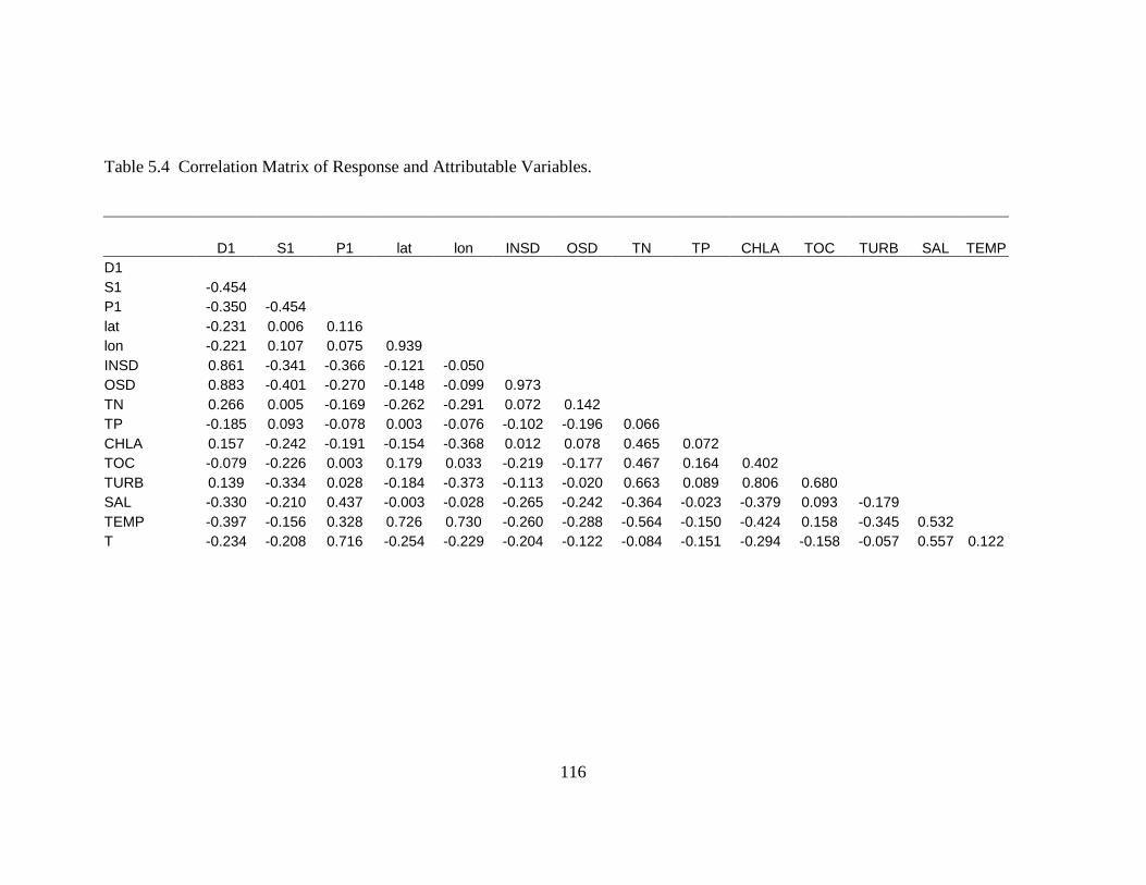
116

Table 5.4 Correlation Matrix of Response and Attributable Variables.

D1 S1 P1 lat lon INSD OSD TN TP CHLA TOC TURB SAL TEMP D1 S1 -0.454 P1 -0.350 -0.454 lat -0.231 0.006 0.116 lon -0.221 0.107 0.075 0.939 INSD 0.861 -0.341 -0.366 -0.121 -0.050 OSD 0.883 -0.401 -0.270 -0.148 -0.099 0.973 TN 0.266 0.005 -0.169 -0.262 -0.291 0.072 0.142 TP -0.185 0.093 -0.078 0.003 -0.076 -0.102 -0.196 0.066 CHLA 0.157 -0.242 -0.191 -0.154 -0.368 0.012 0.078 0.465 0.072 TOC -0.079 -0.226 0.003 0.179 0.033 -0.219 -0.177 0.467 0.164 0.402 TURB 0.139 -0.334 0.028 -0.184 -0.373 -0.113 -0.020 0.663 0.089 0.806 0.680 SAL -0.330 -0.210 0.437 -0.003 -0.028 -0.265 -0.242 -0.364 -0.023 -0.379 0.093 -0.179 TEMP -0.397 -0.156 0.328 0.726 0.730 -0.260 -0.288 -0.564 -0.150 -0.424 0.158 -0.345 0.532 T -0.234 -0.208 0.716 -0.254 -0.229 -0.204 -0.122 -0.084 -0.151 -0.294 -0.158 -0.057 0.557 0.122

117

After choosing the best statistical models using Mallow’s C(p) statistic, we

evaluate their suitability as the best statistical model via their 2R statistic and adjusted

2R statistic.

The coefficient of determination 2R is a criterion used in statistical model

selection. The coefficient of determination 2R is defined by

( )

( )

2

2 1

2

1

1 1

n

i iin

ii

y ySSE

RSST

y y

=

=

−= − = −

−

∑

∑

)

.

SSE is the error sums of squares and SST is the total sums of squares. It measures the

statistical model’s capability to fit the stony coral cover. This value is a measure of the

variation about the mean explained by the regression model. The addition of a new

variable will always increase2R . Thus, the inclusion of a new variable must be checked

to see that it is of statistical significance to the response.

The adjusted 2R is defined by

2 2 11 1 (1 )

1adj

SSEnn p

R RSST n p

n

−−= − = − − − −.

It is a modification of the 2R statistic. This is done by replacing SSE and SST by their

corresponding mean squares which is the division SSE and SST by their corresponding

degrees of freedom, n p− and 1n− respectively. The adjusted2R is not automatically

increased by introducing more variables to the statistical model. If additional variables

are added that do not contribute significantly to the statistical model, this criterion

penalizes the statistical model by lowering the value of the statistic. Thus

adjusted 2R helps in avoiding over fitting the model and must be very close to the

2R statistic.

The best initial statistical model was the four variable model with variables: patch

reef, latitude of the station, total organic carbon and salinity. We identified and ranked

the statistically significant attributable variables in Table 5.5.

118

Table 5.5 Statistical Ranking of the Attributing Variables to Stony Coral Cover.

Rank Variable 2R 1 Patch reef 0.513 2 Latitude of the CREMP station 0.628 3 Salinity 0.691 4 Total organic carbon 0.708

The model with these four attributing variables explains 70.81% of the variation

in the response variable and has an adjusted2R value of 0.66. Since SAL and P1 had a

correlation with each other, we investigated the possibility of multicollinearity using the

variance inflation factor (VIF). Multicollinearity is present if the VIF values are greater

than 10. The VIF of the four attributable variables in our statistical model are close to 1;

therefore, we should not be concerned with the correlation that exists between P1 and

SAL.

5.4.3 Interaction and Higher Order

While the attributable variables in Table 5.5 explain 70.81% of the variation in

the response, to improve the quality of the model we tested for possible contribution to

the stony coral cover by various interactions of the attributable variables. We found that

there are significant interactions between patch reef and latitude, patch reef and total

organic carbon, latitude and total organic carbon, and total organic carbon and salinity.

We ranked the statistically significant attributable interaction variables in Table 5.6.

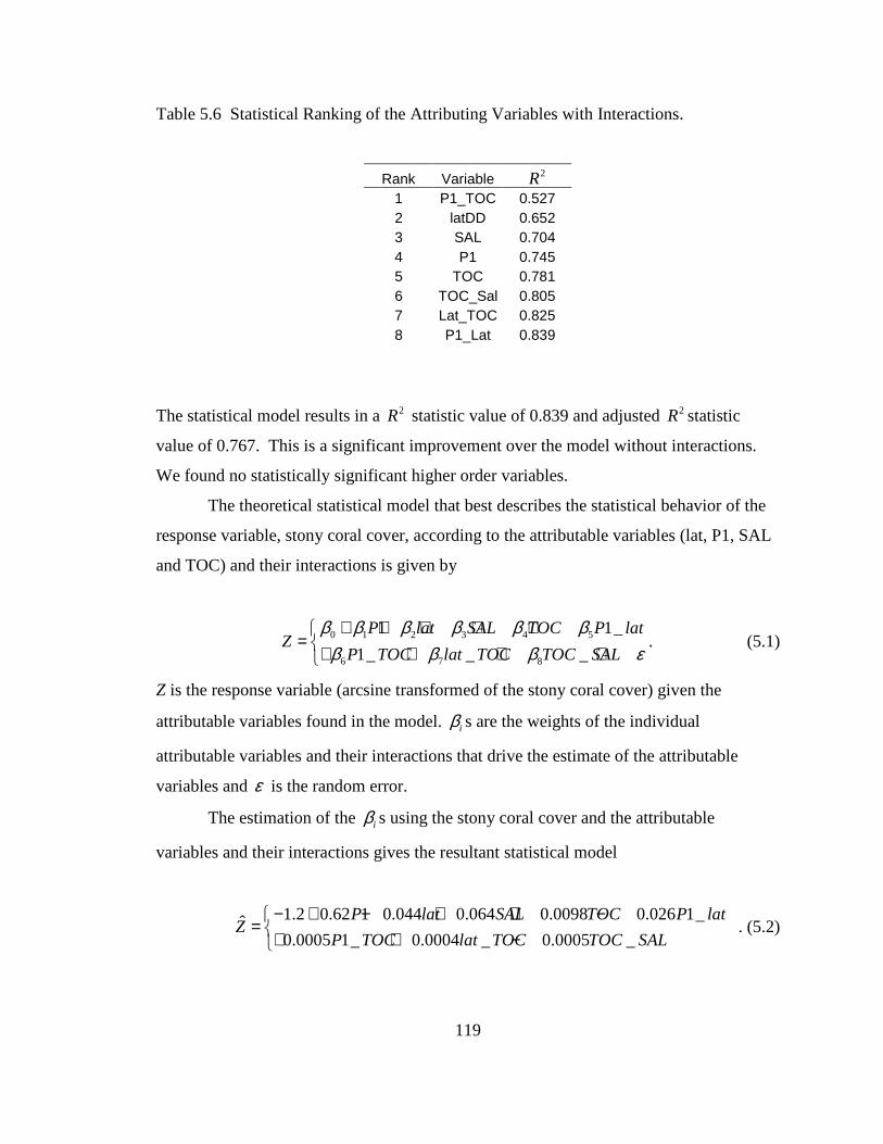
119

Table 5.6 Statistical Ranking of the Attributing Variables with Interactions.

Rank Variable 2R 1 P1_TOC 0.527 2 latDD 0.652 3 SAL 0.704 4 P1 0.745 5 TOC 0.781 6 TOC_Sal 0.805 7 Lat_TOC 0.825 8 P1_Lat 0.839

The statistical model results in a 2R statistic value of 0.839 and adjusted 2R statistic

value of 0.767. This is a significant improvement over the model without interactions.

We found no statistically significant higher order variables.

The theoretical statistical model that best describes the statistical behavior of the

response variable, stony coral cover, according to the attributable variables (lat, P1, SAL

and TOC) and their interactions is given by

0 1 2 3 4 5

6 7 8

1 1_

1_ _ _

P lat SAL TOC P latZ

P TOC lat TOC TOC SAL

β β β β β ββ β β ε

+ + + + += + + + +

. (5.1)

Z is the response variable (arcsine transformed of the stony coral cover) given the

attributable variables found in the model. iβ s are the weights of the individual

attributable variables and their interactions that drive the estimate of the attributable

variables and ε is the random error.

The estimation of the iβ s using the stony coral cover and the attributable

variables and their interactions gives the resultant statistical model

1.2 0.62 1 0.044 0.064 0.0098 0.026 1_ˆ0.0005 1_ 0.0004 _ 0.0005 _

P lat SAL TOC P latZ

P TOC lat TOC TOC SAL

− + − + + −= + + −

. (5.2)

120

where Z is the estimate of the arcsine transformed of the stony coral cover. To obtain the

stony coral cover, we untransformed the Z by

2 ˆsin ( )ˆ0.01

ZY = .

5.4.4 Model Predictive Capability

Of the statistical models investigated, the best is given in equation (5.2). This

model contains the exploratory variables: patch reef, total organic carbon, latitude and

salinity and the interactions between patch reef and latitude, patch reef and total organic

carbon, latitude and total organic carbon, and total organic carbon and salinity. To

investigate how well this model acts as a predictor model, the predictability of the stony

coral cover for 22 stations sampled in 2005 is investigated. The attributable variables,

TOC and salinity, are obtained from the WQMP sampled in the second quarter of 2005.

The observed stony coral cover, P1 and lat are obtained from the CREMP. The results are

given in Table 5.7 as percentage cover.

121

Table 5.7 Prediction Results.

CREMP Type Num WQMP Observed (%) Predicted (%) Turtle P 1 212 6.07 0.45 El Radabob HB 2 220 0.14 2.44 Molasses S 3 225 4.61 1.01 Conch S 4 228 2.28 3.02 Long Key HB 2 242 5.92 18.04 Tennessee D 2 243 5.19 4.72 Tennessee S 2 243 2.55 4.79 W. Turtle Shoal P 1 248 10.74 10.56 Dustan P 2 248 13.20 10.77 Looe Key D 2 263 4.87 5.84 Looe Key S 2 263 4.90 5.81 Conch D 4 264 2.90 1.86 W. Washer Women P 1 269 21.79 14.13 Eastern Sambo D 3 273 4.28 4.60 Eastern Sambo S 3 273 2.26 4.60 Sand Key D 1 281 2.60 8.89 Grecian Rocks S 2 400 2.18 2.05 Porter Patch P 3 400 1.49 1.73 Alligator S 1 401 0.57 5.54 Sombrero S 1 402 4.49 5.52 Western Sambo D 4 403 1.69 4.28 Western Sambo S 4 403 6.58 4.28

The model’s prediction had a 1 to 3 % difference for about 17 of the 22 stations. Good

predictions were observed for various type of reef and high and low stony coral cover.

The worst prediction occurred at Long Key (hardbottom) where the observed value was

about 6 % but the predicted value was 18%. The station with the highest stony coral

cover in the data set was also not predicted properly: observed value of 22 % and the

predicted value was 14%. Most of the medium stony coral covered (2 to 7 % cover)

stations were predicted closely.

122

5.4.5 Final Model

We checked the model, equation (5.2), to see how well it predicted the 2005

values. Since we are satisfied with the model considering the amount of data we had, we

refitted equation (5.2) with the initial 27 values plus the 22 data values. The resulting

model is given by

0.590 0.440 1 0.0038 0.0194 0.0062ˆ 0.0184 1_ 0.00031 1_ 0.000022 _

0.00015 _

P lat SAL TOC

Y P lat P TOC lat TOC

TOC SAL

− + − + += − + −−

This model can now be used to predict the stony coral cover of other areas that have

stony coral cover. To predict stony coral cover, all that is needed for this model is the

latitude (location), type of reef, salinity and total organic carbon.

5.5 Conclusion

Despite the problems we encounter in this study and the limited samples size, this

predictive statistical model for the stony coral cover has shown that it is possible to

formulate a very good predictive model for the stony coral cover.

The statistically significant attributing variables to the predictive statistical model

are latitude (location), patch reef, salinity and total organic carbon. Patch reef contributes

positively to arcsine transformed stony coral cover. This is not surprising as the works by

Tsokos et al. (2006a) showed that since 1996 up to 2005, the patch reefs had the highest

coverage by reef type. Higher latitude shows to have a negative impact on the arcsine

transformed stony coral cover. This again is substantiated by the fact that the high stony

coral coverage are found in the lower keys and Dry Tortugas in the works of Tsokos et al.

(2006a). Salinity has a positive effect to the proportion stony coral cover. Keeping all

other variables in the model constant the proportion stony coral cover increases by 0.0194

for every 1 unit increase in salinity not including its effect in the interaction with total

123

organic carbon. Total organic carbon has a positive contribution of 0.0062 for every unit

increase of TOC while all other variables are kept constant and not including its

contribution due to its interactions with patch reef, latitude and with salinity. This

positive contribution concurs with the chemical properties of TOC, of which colored

dissolved organic matter (CDOM) and particulate organic matter (POM) are two

components. Screening from UV-radiation through light attenuation by suspended POM

(Goreau, McClanahan, Hayes and Strong 1998), or through light absorption by CDOM

(Otis, Carder, English, Ivey and Warrior 2004), can also protect corals from solar-

radiation that sontributes to bleaching events. The interactions between patch and

latitude, latitude and total organic, and salinity and total organic carbon all have a

negative contribution to the proportion stony coral cover. The interaction between patch

and total organic carbon has a positive contribution to the proportion stony coral cover.

A model such as the one formulated here for the FKNMS can be effectively used

in many ways by local managers of reserve sites throughout the world. They can use it to

ensure that influences from developing areas are not affecting the coral reef by measuring

the relevant environment variables. It can also be used in conjunction with GIS mapping

of the habitat areas such as the one that has been done in the Florida Keys. This model

can be used to increase the accuracy of such mapping endeavors. This would also help

governments in locating the best areas to create relevant reserves to ensure the existence

of coral reefs.

124

Chapter 6

Future Research

6.1 Introduction

From the results of the present study, we have identified several interesting and

important extensions for this research.

6.2 Non-Parametric Kernel Density

We will proceed to study the behavior of the bandwidth to obtain better non-

parametric probabilistic estimates of the behavior of the pseudovalues. We will also study

if any other kernel function will give better results of such data. We will seek a

combination of an estimate of the optimal bandwidth and the appropriate kernel function

that will minimize the mean integrated square error. We also propose to investigate the

behavior of the kernel density estimate as a function of sample size.

6.3 Improving the Proposed Statistical Model

We will continue to improve the proposed statistical model by identifying and

testing the significant contributions of additional attributable variables and their

interactions with the ones we have already identified. Attributable variables such as

surface temperature, humidity, rainfall, wind speed, current among others will be

investigated. We believe that these additional attributable variables will significantly

improve the quality of the statistical model.

125

6.4 Surface Response Analysis

We propose to apply surface analysis methodology to the developed model and

any improvements of the subject model. We would like to identify the behavior of the

attributable variables so that we will maximize the response, percent stony coral cover,

with a specified degree of accuracy.

6.5 Stony Coral Cover Parametric Analysis

We will proceed to further investigate the works done by Yanev et al. (2003a, b,

2004) and Tsokos et al. (2005, 2006a) as it pertains to hypothesis testing of the stony

coral cover from over the years for the Coral Reef Evaluation and Monitoring Project.

Since we have identified the probability distribution of the stony coral cover, we can now

proceed to test using parametric analysis as compared to the non-parametric analysis that

was done by Yanev et al. (2003a, b, 2004) and Tsokos et al. (2005, 2006a).

126

References

Andrews, K., Nall, L., Jeffrey, C., and Pittman, S. (2005), "The State of Coral Reef Ecosystems of Florida," 150-200. Angus, J. E. (1994), "Bootstrap One-Sided Confidence Intervals for the Log-Normal Mean," The Statistician, 43, 395-401. Aronson, R. B., and Precht, W. F. (2001), "White-Band Disease and the Changing Face of Caribbean Coral Reefs," Hydrobiologia, 460, 25-38. Baxter, M. J. (2001), "Metodological Issues in the Study of Asssemblage Diversity," American Antiquity, 66, 715-725. Baxter, M. J., Beardah, C. C., and Wright, R. V. S. (1997), "Some Archaeological Applications of Kernel Density Estimates," Journal of Archaeological Science, 24, 347-354. Bean, S. J., and Tsokos, C. P. (1980), "Developments in Nonparametric Density Estimation," International statistical review, 48, 267-287. Bellwood, D. R., Hughes, T. P., Folke, C., and Nystrom, M. (2004), "Confronting the Coral Reef Crisis," Nature, 429, 827-833. Birkeland, C. (1997a), "Implications for Resource Management," in Life and Death of Coral Reefs, ed. C. Birkeland, Norwell, Massachusetts: Kluwer Academic Publishers, pp. 411-435. Birkeland, C. (1997b), "Introduction," in Life and Death of Coral Reefs, ed. C. Birkeland, Norwell, Massachusetts: Kluwer Academic Publishers, pp. 1-12. Boyer, J. N., and Jones, R. D. (2002), "A View from the Bridge: External and Internal Forces Affecting the Ambient Water Quality of the Florida Keys National Marine Sanctuary (Fknms)," in The Everglades, Florida Bay, and Coral Reefs of the Florida Keys. An Ecosystem Sourcebook., eds. J. W. Porter and K. G. Porter, Boca Raton: CRC Press, pp. 609-628. Brown, B. E. (1987), "Worldwide Death of Corals: Natural Cyclic Events or Man-Made Pollution?," Marine Pollution Bulletin, 18, 9-13.

127

Brown, E., Cox, E., Jokiel, P., Rodgers, K., Smith, W., Bissot, B., Coles, S.L., and Hultquist, J. (2004), "Development of Benthic Sampling Methods for the Coral Reef Assessment and Monitoring Program (Cramp) in Hawai'i," Pacific Science, 58, 145-158. Bryant, D., Burke, L., McManus, J., and Spalding, M. (1998), Reefs at Risk a Map-Based Indicator of Threats to the World's Coral Reefs, Washington, D.C.: World Resources Institute. Buddemeier, R. W., Kleypas, J. A., and Aronson, R. B. (2004), "Coral Reefs and Global Climate Change: Potential Contributions of Climate Change to Stresses on Coral Reef Ecosystems.," Technical, Pew Center on Global Climate Change. Buskirk, T. D., and Lohr, S. L. (2005), "A Symptotic Properties of Kernel Density Estimation with Complex Survey," Journal of Statistical Planning and Inference, 128, 165-190. Butler, R. A. (2006), "Coral Reefs and Mangroves Have High Economic Value," mongabay.com. Calitz, F. (1973), "Maximum Likelihood Estimation of the Parameters of the Three Parameter Lognormal Distribution - a Reconsideration," Australian Journal of Statistics, 9, 221-226. Callahan, M. K. (2005), "Distribution of Clionid Sponges in the Florida Keys National Marine Sanctuary (Fknms), 2001-2003," Master's, University of South Florida, College of Marine Science. Callahan, M.K., Wheaton, J., Beaver, C., Brooke, S., Johnson, D., Kidney, J., Kupfner, S., Porter, J.W., Meyers, M., Wade, S., Colella, M., and Bertin, M. (2006), "Coral Reef Evaluation and Monitoring Project 2006 Executive Summary Epa Steering Committee Meeting July 2007," Technical, Florida and Wildlife Research Institute. Carleton, J. H., and Done, T. J. (1995), "Quantitative Video Sampling of Coral Reef Benthos: Large-Scale Application," Coral Reefs, 14, 35-46. Chen, C. (2006), "Tests of Fit for the Three-Parameter Lognormal Distribution," Computational Statistics & Data Analysis, 50, 1418-1440. Cohen, A. C. J. (1951), "Estimating Parameters of Logarithmic-Normal Distributions by Maximum Likelihood," Journal of the American Statistical Association, 46, 206-212. Cohen, A. C. J., and Whitten, B. J. (1980), "Estimation in the Three-Parameter Lognormal Distribution," Journal of the American Statistical Association, 75, 399-404.

128

Connell, J. H., Hughes, T. P., and Wallace, C. C. (1997), "A 30-Year Study of Coral Abundance, Recruitment, and Disturbance at Several Scales in Space and Time.," Ecological Monographs, 67, 461-488. Cummings, B., "Ecology: Distribution and Adaptations of Organisms ", Pearson Education Inc. Datta, S., and Jana, B. B. (2002), "Ecosystem Health Assessment in Five Shallow Tropical Waterbodies " Aquatic Ecosystem Health & Management, 5, 411-421. Davis, G. E. (1982), "A Century of Natural Change in Coral Distribution at the Dry Tortugas: A Comparison of Reef Maps from 1881 and 1976.," Bulletin of Marine Science, 32, 608-623. DOC, U. S. (2003), "Fisheries of the United States, 2002.," Technical, Department of Commerce. Foggo, A., Rundle, S. D., and Bilton, D. T. (2003), "The Net Result: Evaluation Species Richness Extrapolation Techniques for Littoral Pond Invertebrates," Freshwater Biology, 48, 1756-1764 Fox, H. E., Mous, P. S., Pet, J. S., Muljadi, A. H., and Caddwell, R. L. (2005), "Experimental Assessment of Coral Reef Rehabilitation Following Blast Fishing," Conservation Biology, 19, 98-107. Garrison, V.H., Shinn, E.A., Foreman, W.T., Griffin, D.W., Holmes, C.W., Kellogg, C.A., Majewski, M.S., Richardson, L.L., Ritchie, K.B., and Smith, G.W. (2003), "African and Asian Dust: From Desert Soils to Coral Reefs.," BioScience, 53, 469-480. Goreau, T., McClanahan, T., Hayes, R., and Strong, A. (1998), "Conservation of Coral Reefs after the 1998 Global Bleaching Event.," Conservation Biology, 14, 5-15. Goreau, T. F. (1959), "The Ecology of Jamaican Coral Reefs. I. Species Composition and Zonation," Ecology, 40, 67-90. Greenstein, B. J., Curran, H. A., and Pandolfi, J. M. (1998), "Shifting Ecological Baselines and the Demise of Acropora Cervicornis in the Western Atlantic and Caribbean Province: A Pleistocene Perspective.," Coral Reefs, 17, 249-261. Griffin, S. P., Garcia, R. P., and Weil, E. (2003), "Bioerosion in Coral Reef Communities in the Southwest Puerto Rico by the Sea Urchin Echinometra Viridis," Marine Biology, 143, 79-84.

129

Hackett, K. E. (2002), "A Comparative Study of Two Video Analysis Methods to Determine Percent Cover of Stony Coral Species in the Florida Keys," Master's Thesis, University of South Florida, College of Marine Science. Hallock, P. (1997), "Reefs and Reef Limestones in Earth History," in Life and Death of Coral Reefs, ed. C. Birkeland, Norwell, Massachusetts: Kluwer Academic Publishers, pp. 13-42. Hayek, L. C., and Buzas, M.A. (1997), Surveying Natural Populations, New York: Columbia University Press. Heltshe, J. F., and Forrester, N.E. (1985), "Statistical Evaluation of the Jackknife Estimate of Diversity When Using Quadrat Samples," Ecology, 66, 107-111. Hill, B. M. (1963), "The Three-Parameter Lognormal Distribution and Bayesian Analysis of a Point-Source Epidemic," Journal of the American Statistical Association, 58, 206-212. Hinrichsen. (1997), "Coral Reefs in Crisis," BioScience, 47, 554-558. Hodges, A., Mulkey, D., Philippakos, E., and Adams, C. (2006), "Economic Impacts of Agricultural and Natural Resource Industries in Florida, 2003," EDIS, FE627. Hodgson, G. (1999), "A Global Assessment of Human Effects on Coral Reefs.," Marine Pollution Bulletin, 38, 345-355. Hubbard, D. K. (1997), "Reefs as Dynamic Systems," in Life and Death of Coral Reefs, ed. C. Birkeland, Massachusetts: Kluwer Academic Publishers, pp. 43-67. Hughes, T. P., and Tanner, J. E. (2000), "Recruitment Failure, Life Histories, and Long-Term Decline of Caribbean Corals.," Ecology, 81, 2250-2263. Hunter, I. G., and Jones, B. (1996), "Coral Associations of the Plesitocene Ironshore Formation, Grand Cayman," Coral Reefs, 15, 249-267. Jaap, W. C. (2000), "Coral Reef Restoration," Ecological Engineering, 15, 345-364. Jackson, J. B. C. (1992), "Pleistocene Perspectives of Coral Reef Community Structure," American Zoologist, 32, 719-731. Jackson, J.B.C., Kirby, M.X., Berger, W.H., Bjorndal, K.A., Botsford, L.W., Bourque, B.J., Bradbury, R.H., Cooke, R., Erlandson, J., Estes, J.A., Hughes, T.P., Kidwell, S., Lange, C.B., Lenihan, H.S., Pandolfi, J.M., Peterson, C.H., Steneck, R.S., Tegner, M.J., and Warner, R.R. (2001), "Historical Overfishing and the Recent Collapse of Coastal Ecosystems," Science, 293, 629-638.

130

Johannes, R. E., and Riepen, M. (1995), "Environmental, Economic and Social Implications of the Live Fish Trade in Asia and the Western Pacific," Technical, The Nature Conservancy Coastal and Marine Program. Johns, G. M., Leeworthy, V. R., Bell, F. W., and Bohn, M. A. (2003), "Socioeconomic Study of Reefs in Southeast Florida, Final Report," Technical, Broward County, Palm Beach County, Miami-Dade County, Monroe County, Florida Fish and Widlife Conservation Commission, National Oceanic and Atmospheric Administration. Jørgensen, S. E., Costanza, R., and Xu, F. (eds.) (2005), Handbook of Ecological Indicators for Assessment of Ecosystem Health, Boca Raton, FL: CRC Press. Keller, B. D., and Itkin, A. (2002), "Shoreline Nutrients and Chlorophyll a in the Florida Keys, 1994-1997: A Preliminary Analysis.," in The Everglades Florida Bay and Coral Reefs of the Florida Keys: An Ecosystem Sourcebook, ed. J. W. Porter, Porter, K. G., Boca Raton, FL.: CRC Press, pp. 649-658. Ker, A. P., and Goodwin, B. K. (2000), "Nonparametric Estimation of Crop Insurance Rates Revisited," American Journal of Agricultural Economics, 82, 463-478. Krebs, C. J. (1999), Ecological Methodology, Menlo Park , CA: Addison- Wesley Educational Publishers, Inc. Land, C. E. (1971), "Confidence Intervals for Linear Functions of the Normal Mean and Variance," The Annals of Mathematical Statistics, 42, 1187-1205. Land, C. E. (1972), "An Evaluation of Approximate Confidence Interval Estimation Methods for Lognormal Means," Technometrics, 14, 145-158. Land, C. E. (1974), "Confidence Interval Estimation for Means after Data Transformations to Normality," Journal of American Statistical Association, 69, 1187-1205. Lapointe, B. E., and Thacker, K. (2002), "Community-Based Water Quality and Coral Reef Monitoring in the Negril Marine Park, Jamaica: Land-Based Nutrient Inputs and Their Ecological Consequences," in The Everglades Florida Bay and Coral Reefs of the Florida Keys: An Ecosystem Sourcebook, ed. J. W. Porter, Porter, K. G., Boca Raton, FL.: CRC Press, pp. 939-963. Lessios, H. A. (1988), "Mass Mortality of Diadema Antillarum in the Caribbean: What Have We Learned?," Annual Review of Ecology and Systematics, 19, 371-393. Lirman, D. G., Gracias N. R., Gintert, B. E., Gleason, A.C.R., Reid, R.P., Negahdaripour, S., and Kramer, P. (2007), "Development and Application of a Video-Mosaic Survey Technology to Document the Status of Coral Reef Communities," Environmental Monitoring and Assessment, 125, 59-73.

131

Liu, K. (1998), "Kernel Estimates of Statistical Distribution Function," Dissertation, University of South Florida, Mathematics and statistics. Liu, K., and Tsokos, C. P. (2002), "Optimal Bandwidth Selection for a Nonparametric Estimate of the Cumulative Distribution Function," International Journal of Applied Mathematics, 10, 33-50. Loft, K. (2008), "The Fading of the Reefs," The Tampa Tribune, 4. Lotti, F., and Santarelli, E. (2004), "Industry Dynamics and the Distribution of Firm Sizes: A Nonparametric Approach," Southern Economics Journal, 70, 443-466. Macintyre, I. G. (1988), "Modern Coral Reefs of Western Atlantic: New Geological Perspective.," American Association of Petroleum Geologists Bulletin, 72, 1360-1369. Mesolella, K. J. (1968), "The Uplift Reefs of Barbados: Physical Stratigraphy, Facies Relationships and Absolute Chronology," Dissertation, Brown University. Miller, R. G. (1974), "The Jackknife--a Review," Biometrika, 61, 1-15. Mohn, E. (1979), "Confidence Estimation of Measures of Location in the Log Normal Distribution," Biometrika, 66, 567-575. Murdoch, T. J. T., and Aronson, R.B. (1999), "Scale-Dependent Spatial Variability of Coral Assemblages Along the Florida Reef Tract," Coral Reefs, 18, 341-351. Otis, D., Carder, K., English, D., Ivey, J., and Warrior, H. (2004), "Cdom Transport from the Bahamas Banks.," Coral Reefs, 23, 152-160. Overton, W. S., White, D., and Stevens, D.L. (1991), "Design Report for the Environmental Monitoring Assessment Program (Emap)," Technical Report EPA/600/3-91/053 US EPA. Pandolfi, J. M. (1996), "Limited Membership in Pleistocene Reef Coral Assembages from Huon Peninsula, Papua New Guinea: Constancy During Global Change," Paleobiology, 22, 152-176. Pandolfi, J. M., and Jackson, J. B. C. (1997), "The Maintenance of Diversity on Coral Reefs: Examples from the Fossil Record.," in Eighth International Coral Reef Symposium Panama, pp. 397-404. Pandolfi, J. M., and Jackson, J. B. C. (2001), "Community Structure of Pleistocene Coral Reefs of Curacao, Netherlands, Antilles.," Ecological Monographs, 71, 49-67.

132

Pandolfi, J. M., and Jackson, J. B. C. (2007), "Broad-Scale Patterns in Pleistocene Coral Reef Communities from the Cribbean: Implications for Ecology and Management," in Geological Approaches to Coral Reef Ecology, ed. R. B. Aronson, New York, NY: Springer, pp. 201-236. Pante, E., King, A., and Dustan, P. (2007), "Short-Term Decline of a Bahamian Patch Reef Coral Community: Rainbow Gardens Reef 1991-2004," Hydrobiologia, online. Paulay, G. (1996), "Diversity and Distribution of Reef Organisms," in Life and Death of Coral Reefs, ed. C. Birkeland, Massachusetts: Kluwer Academic Publishers, pp. 298-353. Pavlov, D.S., Smurov, A.V., Il'yash,L.V., Matorin, D.N., Kluyev,N.A., Kotelevtsev, S.V., Rumak, V.S., and Smurova, T.G.. (2004), "Present-Day State of Coral Reefs of Nha Trang Bay (Southern Vietnam) and Possible Reasons for the Disturbance of Habitats of Scleractinian Corals," Russian Journal of marine Biology, 30, 43-50. Peters, E. C. (1997), "Diseases of Coral-Reef Organisms.," in Life and Death of Coral Reefs, ed. C. Birkeland, Norwell, Massachusetts: Kluwer Academic Publishers, pp. 68-95. Pinckney, J. L., Paerl, H. W., and Valdes-Weaver, L. M. (2005), "Using Phytoplankton Photopigments as a Bioindicator for the Condition of Estuarine Ecosystems," ERF 2005. Porter, J. W., Lewis, S. K., and Porter, K. G. (1999), "The Effect of Multiple Stressors on the Florida Keys Coral Reef Ecosystem: A Landscape Hypothesis and a Physiological Test," Limnology and Oceanography, 44, 941-949. Porter, J. W., Vladimir, K., Patterson, K.L., Porter, K.G.,Japp, W. C., Wheaton, J.L., Hackett, K., Lybolt, M., Tsokos, C.P., Yanev, G., Marcinek,.M., Dotten, J., Eaken, D., Patterson, M., Meier, O.W., Brill, M., Dustan, P. (2002), "Detection of Coral Reef Change by the Florida Keys Coral Reef Monitoring Project," in The Everglades Florida Bay and Coral Reefs of the Florida Keys: An Ecosystem Sourcebook, ed. J. W. Porter, Porter, K. G., Boca Raton, FL.: CRC Press, pp. 749-769. Research. (2008), "Historic Economic Impact." Riegl, B. (2007), "Extreme Climatic Events and Coral Reefs: How Much Short-Term Threat from Global Change?," in Geological Approaches to Coral Reef Ecology, ed. R. B. Aronson, New York, NY: Springer, pp. 315-341. Rogers, C. S., Gilnack, M., and Fitz III, H. C. (1983), "Monitoring of Coral Reefs with Linear Transects: A Study of Storm Damage," Journal of Experimental Marine Biology and Ecology, 66, 285-300.

133

Rosenblatt, M. (1956), "Remarks on Some Nonparametric Estimates of a Density Function," Annals of Mathematical Statistics, 27, 832-837. Routledge, R. D. (1980), "Bias in Estimating the Diversity of Large, Uncensused Communities," Ecology, 61, 276-281. Santavy, D.L., Mueller, E., Peters, E.C., MacLaughlin, L., Porter, J., Patterson, K.L., and Campbell, J. (2001), "Quantitative Assessment of Coral Diseases in the Florida Keys: Strategy and Methodology," Hydrobiologia, 460, 39-52. Santavy, D. L., Summers, J. K., Engle, V. D., and Harwell, L. C. (2005), "The Conditions of Coral Reefs in South Florida (2000) Using Coral Disease and Bleaching as Indicators.," Enviromental Monitoring and Assessment, 100, 129-152. Shannon, C. E. (1948), "A Mathematical Theory of Communication " Bell system technical journal, 27, 379-423, 623-656. Shinn, E.A., Smith, G.W., Prospero, J.M., Betzer, P., Hayes, M.L., Garrison, V., and Barber, R.T. (2000), "African Dust and the Demise of Caribbean Coral Reefs.," Geophysical Research Letters, 27, 3029-3032. Silverman, B. W. (1986), Density Estimation for Statistics and Data Analysis, New York, NY: Chapman and Hall. Simpson, E. H. (1949), "Measurement of Diversity," Nature, 163, 688. Sokal, R. R., and Rohlf, F.J. (1995), Biometry (3rd ed.), New York: W.H. Freeman and Company. Spellerberg, I. F. (2005), Monitoring Ecological Change (2nd ed.), United Kingdom: Cambridge University Press. Stephens, M. A. (ed.) (1986), Tests Based on Edf Statistics (Vol. Chapter 4), ed. R. B. D'Agostino, Stephens, M.A., New York: Marcel Dekker, INC. Talaue-McManus, L., and Kesner, K. P. N. (1993), "Valuation of a Philippine Municipal Sea Urchin Fishery and Implications of Its Collapse," in Fourth Annual Common Property Conference, Manila, Philippines: Coastal Resources Research Network, pp. 229-239. Tapia, R. A., and Thompson, R. J. (1978), Nonparametric Probability Density Estimation, London: The Johns Hopkins University Press. Tian, L., and Wu, J. (2006), "Confidence Intervals for Mean of Lognormal Data with Excess Zeros," Biometrical Journal, 48, 149-156.

134

Tsokos, C. P., Hoare, A. J., and Yanev, G. P. (2005), "Statistical Analysis of Florida Keys Coral Reef Data (1996-2004 Video Point Count Data)," Technical, US EPA Florida Keys National Marine Sanctuary Water Quality Protection Program, Florida Marine Institute. Tsokos, C. P., Hoare, A. J., and Yanev, G. P. (2006a), "Statistical Analysis of Florida Keys Coral Reef Data (1996-2005 Video Point Count Data)," Technical, US EPA Florida Keys National Marine Sanctuary Water Quality Protection Program, Florida Marine Institute. Tsokos, C. P., Hoare, A. J., and Yanev, G. P. (2006b), "Statistical Analysis of Species Inventory and Disease/Condition Coral Reef Data, 1996-2005," Technical, US EPA Florida Keys National Marine Sanctuary Water Quality Protection Program, Florida Fish and Widlife Research Institute. Tukey, J. (1958), "Bias and Confidence in Not Quite Large Samples (Abstract)," Annals of Mathematical Statistics, 29, 614. Urquhart, N. S., and Kincaid, T. M. (1999), "Designs for Detecting Trend from Repeated Surveys of Ecological Resources," Journal of Agricultural, Biological, and Emvironmental Statistics, 4, 404-414. Wellington, G. M., and Glynn, P. W. (2007), "Responses of Coral Reefs to El Nino-Southern Oscillation Sea-Warming Events," in Geological Approaches to Coral Reef Ecology, ed. R. B. Aronson, New York, NY: Springer, pp. 342-385. Westmacott, S., Teleki, K., Wells, S., and West, J. (2000), Management of Bleached and Severly Damaged Coral Reefs., Gland, Switzerland, and Cambridge, UK.: IUCN. Wheaton, J., Jaap, W.C., Porter, J.W., Kosmynin, V., Hackett, K.E., Lybolt, M., Callahan, M.K., Kidney, J., Kupfner, S., Tsokos, C.P., and Yanev, G. (2001), "Epa/Fknms Coral Reef Monitoring Project Executive Summary 2001," in FKNMS Symposium: An Ecosystem Report Card, Washington D.C., December 2001: Florida Marine Research Institute IHR2001-004. , p. 19. Wielgus, J., Chadwick-Furman, N. E., and Dubinsky, Z. (2004), "Coral Cover and Partial Mortality on Anthropogenically Impacted Coral Reefs at Eilat, Northern Red Sea," Marine Pollution Bulletin, 48, 248-253. Wilkinson, C. (2002), "Status of Coral Reefs of the World:2002," Technical, Austrialian Institute of Marine Science.

135

Wolf, C. A., and Sumner, D. A. (2001), "Are Farm Sixe Distribution Bimodal? Evidence from Kernel Density Estimates of Dairy Farm Size Distributions," American Journal of Agricultural Economics, 83, 77-88. Wood, R. (2007), "The Changing Fate of Coral Reefs: Lessons from the Deep Past," in Geological Approaches to Coral Reef Ecology, ed. R. B. Aronson, New York, NY: Springer, pp. 3-27. Xu, F. (1996), "Ecosystem Health Assessment of Lake Chao, a Shallow Eutrophic Chinese Lake," Lakes & Reservoirs: Research & Management, 2, 101–109 Yanev, G. P., and Tsokos, C. P. (2003a), "Statistical Analysis of Florida Keys Coral Reef Data (1996-2002 Video Point Count Data)," Technical, US EPA Florida Keys National Marine Sanctuary Water Quality Protection Program, Florida Marine Institute. Yanev, G. P., and Tsokos, C. P. (2003b), "Statistical Analysis of Florida Keys Coral Reef Data :1996-2001 (Video Transects) and 1996-2002 (Species Inventory and Disease) " Technical, US EPA Florida Keys National Marine Sanctuary Water Quality Protection Program, Florida Marine Institute. Yanev, G. P., and Tsokos, C. P. (2004), "Statistical Analysis of Florida Keys Coral Reef Data (1996-2003 Video Point Count Data)," Technical, US EPA Florida Keys National Marine Sanctuary Water Quality Protection Program, Florida Marine Institute. Zahl, S. (1977), "Jackknifing an Index of Diversity," Ecology, 907-913. Zar, J. H. (1996), Biostatistical Analysis (3rd ed.), Upper Saddle River, New Jersey: Prentice-Hall, Inc. Zhou, X., and Gao, S. (1997), "Confidence Intervals for the Lognormal Mean," Statistics in Medicine, 16, 783-790. Zhou, X., and Gao, S. (2000), "One-Sided Confidence Intervals for Means of Positively Skewed Distributions," The American Statistician, 54, 100 -104. Zhou, X., and Tu, W. (2000), "Confidence Intervals for the Mean of Diagnostic Test Charge Data Containing Zeros," Biometrics, 56, 1118-1125.

About The Author

Armando J. Hoare was born in Corozal Town, Belize, Central America, the ninth child of

11 siblings. In 1992 he graduated magna cum laude with his Bachelor of Science degree

in Mathematics and Chemistry from Regis University, Colorado. He taught mathematics

for 10 years at St. John’s Junior College, served as department head for two years and

was awarded Teacher of the Year in 1998.

In 2002, Armando received his Master of Education in Educational Leadership

from the University of North Florida with a distinction in mathematics. He achieved a

Master of Arts in Mathematics at the University of South Florida. He then pursued his

doctoral degree focusing on Statistics. During his time as a graduate student, Armando

received a certificate of recognition for outstanding performance as a graduate teaching

assistant, and was nominated for the Provost’s Award. Armando is married to Ana and

they have a son, Armando Fulgencio.