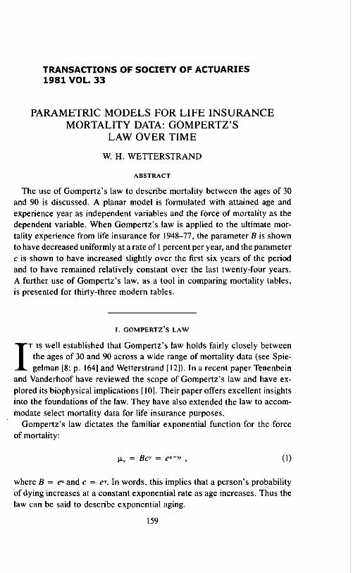
TRANSACTIONS OF SOCIETY OF ACTUARIES 1981 VOL. 33

PARAMETRIC MODELS FOR LIFE INSURANCE MORTALITY DATA: GOMPERTZ'S

LAW OVER TIME

W. H. WETTERSTRAND

ABSTRACT

The use of Gompertz's law to describe mortality between the ages of 30 and 90 is discussed. A planar model is formulated with attained age and experience year as independent variables and the force of mortality as the dependent variable. When Gompertz's law is applied to the ultimate mor- tality experience from life insurance for 1948-77, the parameter B is shown to have decreased uniformly at a rate of I percent per year, and the parameter c is shown to have increased slightly over the first six years of the period and to have remained relatively constant over the last twenty-four years. A further use of Gompertz's law, as a tool in comparing mortality tables, is presented for thirty-three modern tables.

I. GOMPERTZ'S LAW

I T IS well established that Gompertz's law holds fairly closely between

the ages of 30 and 90 across a wide range of mortality data (see Spie- gelman [8: p. 164] and Wetterstrand [12]). In a recent paper Tenenbein

and Vanderhoof have reviewed the scope of Gompertz's law and have ex-

plored its biophysical implications [ 10]. Their paper offers excellent insights into the foundations of the law. They have also extended the law to accom- modate select mortality data for life insurance purposes.

Gompertz's law dictates the familiar exponential function for the force of mortality:

I~y = B c .~ = e ~+~y , (1)

where B = e" and c = e~. In words, this implies that a person's probability of dying increases at a constant exponential rate as age increases. Thus the law can be said to describe exponential aging.

159

160 PARAMETRIC MODELS FOR MORTALITY DATA

If we apply the natural logarithmic transformation to equation (1), a linear equation results:

In ixy = a + 3'Y. (2)

The familiar textbook approximation can be used to estimate the force of mortality from observed mortality rates [2: p. 17]:

~y+l/2- - l n ( l - qy). (3)

One of the consequences of formula (2) is that a force of mortality satisfying Gompertz 's law has a linear graph when plotted on semilog paper. Miller recommends the plotting of observed mortality rates in this way and notes that others have recommended that graduation processes be applied to a logarithm of the observed rates plus a constant. [3: pp. 14, 15, 46, 48]. Ruth showed that the application of linear least squares to formula (2) is an effective way of determining B and c [6]. Tenenbein and Vanderhoof ad- vocate applying weighted linear least squares to formula [2], using as weights the number of deaths making up the numerator in the mortality rate.

One advantage of applying linear least squares to formula (2) is that the result is of the form

l n l x , = & + '~y + ~ . , (4)

where & and ¢/are determined in such way that the~. 's are minimal in the least-squares sense; that is, the sum of their squares is minimal. When the exponential transformation is applied to formula (4), the result represents the desired fitted model:

~., = ~.,d,., (5)

where Ay = e a÷~ are the fitted values. The point to be made from formula (5) is that if the~, 's are minimized in formula (4) the relative (or percentage) error in formula (5) is minimized, the relative error being contained in the term e~,. Thus, minimizing the absolute error in formula (4) is equivalent to minimizing the relative error in formula (5). This is important when dealing with data that vary as much in magnitude as mortality data do.

A computer program named GOMPQ has been written to accept mortality rates as input and produce a graph on a video plotter with photostatic copier. The graph contains approximate values of the forces of mortality, along with

PARAMETRIC MODELS FOR MORTALITY DATA 161

a regression line fitted to them, be tween the ages of 30 and 90. The program

uses unweighted linear least squares to est imate In ~.y+~. (Weighted least

squares will be used in future studies, when possible.) The observed , fitted,

and residual values of ~y,~2 are printed out along with the est imates of B,

c, and the multiple regression coefficient be tween the observed and fitted

values of In p.y+ ~. A program with identical output, called U S L I F E , accepts

United States census and mortali ty data (Pv and D~.) as input, and forms qy

from the formula in Grevil le [l]:

D~, (6) qY = 3Py - V2Dy"

These two programs allow one to process a set of mortali ty data quite easily

in five minutes or less at a graphic terminal.

11. EXAMPLES

The applicability of G o m p e r t z ' s law to life insurance mortal i ty data can

be explored by considering the results of using G O M P Q to analyze the

following sets of data:

1. 1930--40 experience, which was the basis for the Commissioners 1941 Standard Ordinary Mortality Table [9].

2. 1950-54 experience, which was the basis for the Commissioners 1958 Standard Ordinary Mortality Table [9].

3. 1970-75 experience separated by sex, which is the basis for the K-tables proposed as new standards for life insurance valuation [7].

These results are shown graphically in Figures 1-4. The Gomper t z con-

stants and corresponding complete expecta t ions of life at age 30 are shown

in Table 1. Good Gomper tz fits be tween ages 30 and 90 can be seen in Figures I-3.

Figures 1 and 2 represent predominant ly male mortality, and Figure 3 rep-

TABLE 1

COMBINED, ULTIMATE EXPERIENCE FOR LIFE INSURANCE: COMPARISON OF PARAMETERS OVER FOUR TIME PERIODS

1930-40 .1326 !.089 38.89 1950-54 .0569 1.098 43.65 1970-75, male .0416 1.100 45.55 1970-75, female . . . . . . . . . . . . 0312 1.097 50.29

10 ~

l0 ~ •

i,0

I

10-, I I I I I I I I I l0 20 30 40 50 60 70 80 90 100

Attained Age

FIG. l . - - - -Combined, ult imate experience for life insurance: force of mortality by

age for 1930--40 anniversaries .

103

10 2 -

IO

_

I - +

lO-' I I I I I I I I I 10 20 30 40 50 60 70 80 90 100

Attained Age

FiG. 2 . - - -Combined , ultimate exper ience for life insurance: force of mortality by

age for 1950-54 anniversar ie s .

162

10 ~

+

102

i,o

l ' + ' 4 - +

+

io- , I I I I I I 0 10 20 30 40 50 60 70 80 90 100

Attained Age

FIe;. 3 . - - M a l e , ultimate experience for life insurance: force of mortality by age for 1970-75 anniversar ie s .

10 ~

102 -

l0

I - ' =

10-'

0

+.

-I- + +

I I I I I I I I I 10 20 30 40 50 60 70 80 90 100

Attained Age

FIG. 4 . - - F e m a l e , u l t imate e x p e r i e n c e for life insu rance : force o f mor ta l i ty by age

for 1970-75 ann ive r sa r i e s .

163

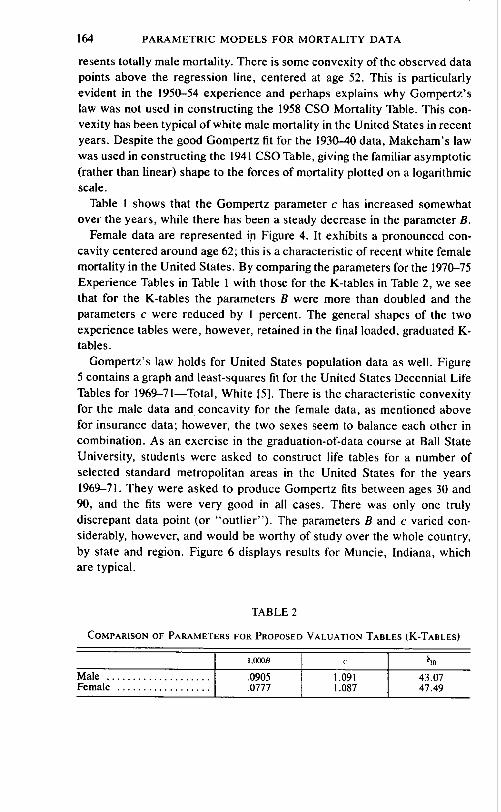
164 PARAMETRIC MODELS FOR MORTALITY DATA

resents totally male mortality. There is some convexity of the observed data points above the regression line, centered at age 52. This is particularly evident in the 1950--54 experience and perhaps explains why Gompertz's law was not used in constructing the 1958 CSO Mortality Table. This con- vexity has been typical of white male mortality in the United States in recent years. Despite the good Gompertz fit for the 1930-40 data, Makeham's law was used in constructing the 1941 CSO Table, giving the familiar asymptotic (rather than linear) shape to the forces of mortality plotted on a logarithmic scale.

Table 1 shows that the Gompertz parameter c has increased somewhat over the years, while there has been a steady decrease in the parameter B.

Female data are represented in Figure 4. It exhibits a pronounced con- cavity centered around age 62; this is a characteristic of recent white female mortality in the United States. By comparing the parameters for the 1970-75 Experience Tables in Table I with those for the K-tables in Table 2, we see that for the K-tables the parameters B were more than doubled and the parameters c were reduced by ! percent. The general shapes of the two experience tables were, however, retained in the final loaded, graduated K- tables.

Gompertz's law holds for United States population data as well. Figure 5 contains a graph and least-squares fit for the United States Decennial Life Tables for 1969-71--Total, White [5]. There is the characteristic convexity for the male data and concavity for the female data, as mentioned above for insurance data; however, the two sexes seem to balance each other in combination. As an exercise in the graduation-of-data course at Bali State University, students were asked to construct life tables for a number of selected standard metropolitan areas in the United States for the years 1969-71. They were asked to produce G0mpertz fits between ages 30 and 90, and the fits were very good in all cases. There was only one truly discrepant data point (or "outlier"). The parameters B and c varied con- siderably, however, and would be worthy of study over the whole country, by state and region. Figure 6 displays results for Muncie, Indiana, which are typical.

TABLE 2

COMPARISON OF PARAMETERS FOR PROPOSED VALUATION TABLES (K-TABLES)

1.000B c

Male .0905 1.091 Female . . . . . . . . . . . . . . . . . . . . 0777 1.087

~30

43.07 47.49

lO ~

10 ~

~ to t-

io-, I I I I I I I I I 0 10 20 30 40 50 60 70 80 90 100

Attained Age

FIG. 5.--United States Life Table for 1969-71--Total, White: force of mortality by

• age.

|0 ~

0

lO 2

l0

+

I

I I I I I I I I I I 0 20 30 40 50 60 70 80 90 100

Attained Age

FIG. 6.--1969-71 Life Table for Muncie, Indiana: force of mortality by age

10-1

166 PARAMETRIC MODELS FOR MORTALITY DATA

1II. SOCIETY OF ACTUARIES CONTINUING STUDY OF ULTIMATE MORTALITY

The Society of Actuaries, in its annual Reports of Mortality and Morbidity Experience, has published mortality data for standard issues, by attained age, for policy years 16 and over combined, on an annual basis for each experience year beginning with the period between 1947 and 1948 policy anniversaries and continuing to the present. This is the most homogeneous, regular body of mortality data available in which to observe annual changes. For this paper, data for thirty policy years, beginning with the year ending on the 1948 policy anniversary and concluding with the year ending on the 1977 policy anniversary, were studied separately with particular reference to the applicability of Gompertz ' s law to such data. The experience years are labled 1948-77 in this paper. The label 1948, for example, is used to identify experience between 1947 and 1948 anniversaries, with midpoint January I, 1948.

A program similar to GOMPQ was used to analyze each year 's data separately, fitting Gompertz ' s law to the forces of mortality with unweighted least squares. Data for 1976-77 anniversaries were analyzed separately with GOMPQ. Three typical graphs are presented in Figures 7-9, corresponding

10 ~ +

I I F -

10 "--:

o

y 10-, I I I I I I I l I

10 20 30 40 50 60 70 80 90 100

Attained Age

FIG. 7.---Combined, ultimate experience for life insurance: force of mortality by age for 1947-48 anniversaries.

10 3

102 -

.-_ -

!

,k

]o-' I I ~ l l l l l l l l l l l l l l ~ t l l l l l l l l l l l l l , l l l l l l l l l l l l l l l l 10 20 30 40 50 60 70 80 90 100

Attained Age

FtG. 8 . - - C o m b i n e d , u l t ima te e x p e r i e n c e for life in su rance : force of mor t a l i t y by

age for 1962--63 ann ive r s a r i e s .

10 3

102 -

o o o

I

0 10 20 30 40 50 60 70 80 90 100

Attained Age

FiG. 9 . - - -Combined , u l t ima te e x p e r i e n c e for life i n su rance : force o f mor t a l i t y by

age for 1975-76 ann ive r s a r i e s .

168 PARAMETRIC MODELS FOR MORTALITY DATA

TABLE 3

COMBINED, ULTIMATE EXPERIENCE FOR LIFE INSURANCE: COMPARISON OF PARAMETERS FROM 1947--48 TO 1976-77

Year L00os c ~0 Year 1,000B c I ~30

1948 . . . . . 074 1.095 42.7 1963 . . . . . 049 1.099 44.5* 1949 . . . . . 072 1.095 43.0 1964 . . . . . 055 1.097 44.5 1950 . . . . . 070 1.095 43.5 1965 . . . . . 054 1.097 44.7 1951 . . . . . 069 1.095 43.3* 1966 . . . . . 052 1.098 44.8 1952 . . . . . 073 1.094 43.7 1967 . . . . . 050 1.098 44.8

1953 . . . . . 068 1.095 43.7 1968 . . . . . 048 1.099 44.8 1954 . . . . . 061 1.097 43.8 1969 . . . . . 053 1.097 45.0 1955 . . . . . 057 1.097 44.0 1970 . . . . . 054 1.096 45.3 1956 . . . . . 056 1.097 44.2 1971 . . . . . 050 1.097 45.5 1957 . . . . . 050 1.099 44.2 1972 . . . . . 048 1.098 45.6

1958 . . . . . 055 1.098 44.2 1973 . . . . . 044 1.099 45.6 1959 . . . . . 050 1.099 44.4 1974 . . . . . 046 1.098 45.8 1960 . . . . . 046 1.100 44.4 1975 . . . . . 044 1.098 46.3 1961 . . . . . 051 1.098 44.6 1976 . . . . . 041 1.099 46.7 1962 . . . . . 049 1.099 44.6 1977 . . . . . 043 1.098 46.6*

*Decreased from previous year.

to the e x p e r i e n c e y e a r s 1948, 1963, and 1976, respec t ive ly . Cha rac t e r i s t i c

c o n v e x i t y can be o b s e r v e d fo r 1948 and 1963, bu t no t fo r 1976. T h e va lues

o f the p a r a m e t e r s 1,000B and c, a long wi th ~30, are s h o w n in Table 3 fo r all

yea r s . T h e r e is a fair ly u n i f o r m d e c r e a s e in the p a r a m e t e r 1,000B o v e r the

y e a r s , f r o m 0.074 in 1948 to 0.043 in 1977. T h e r e is one s h a r p b r eak in the

va lue s o f c b e t w e e n 1953 and 1954. Af te r 1954, c s t ays b e t w e e n 1.096 and

1.100. F r o m these da ta w e see that G o m p e r t z ' s law ho lds qui te c lose ly in

annua l c r o s s s ec t i ons o f the mor ta l i t y sur face . We will n o w inves t iga te tha t

su r f ace in its ent i re ty.

IV. PLANAR MODELS INCORPORATING TIME TRENDS

T w o v e r s i o n s o f a t h r e e - d i m e n s i o n a l model have been f o r m u l a t e d , each

wi th t w o i n d e p e n d e n t va r iab les :

1. Attained age y, which is time from birth.

2. Two alternative time measures:

a) Experience year s, which is time from the base year (1900).

b) Birth year, u = s - y, which is constant for any individual, measured from the

base year (1900).

P a r a m e t e r s in the mode l inc lude the fol lowing:

1. B0, the Gompertz location parameter for the base year (1900).

PARAMETRIC MODELS FOR MORTALITY DATA 169

2. c, the Gompertz aging parameter. 3. d, a new parameter to allow discounting of B with respect to time.

Two equivalent models are considered here. They are both extensions of Gompertz's law and correspond to using the two time measures described above. The first model is

p,y., = B o d ~ c y = B , c ~ ' , (7)

where B, (= B o d O varies by experience year but c does not. The second model results from a simple reparameterization of the first:

p.:.u = Bod'~ : = B u O , (8)

where Bu (= B o d O varies by birth year (or cohort) and ~ = c d . Since the two are equivalent, we will concentrate on the experience year in fitting a planar model to the data considered in the previous section.

We first transform formula (7) into exponential form:

p.y., = e "+a'÷vr , (9)

where Bo = e% d = e~, and c = ev. Taking the natural logarithm of formula (9) yields

In p.~;, = a + {3s + 7 Y . (lO)

This expression represents a plane for ~,., Figure 10 shows the surface of In ~y,~ for the data considered previously

covering the years 1948-76. At first glance it seems quite planar, almost dull. There is some jaggedness at the higher ages, and a slight hump at the middle ages for the earlier years.

Unweighted least-squares analyses were performed on the data, using the model in formula (10) for two time periods: 1948-76 and 1954-76. Because

of the break in the value of c around 1954, noted in the univariate analyses, the fit of the model for the second time period was found to be slightly better than for the first time period.

The values of the parameters for both time periods are shown in Table 4. The values of c are in the range established previously by the univariate analyses. The parameter d corresponds to a rate of discount of about l percent per year. The parameter B0 is arbitrary, since it depends on the

choice of the base year.

170 PARAMETRIC MODELS FOR MORTALITY DATA

The fit o f the planar model can be judged from the residuals, or deviat ions

of the obse rved values of In p.y., f rom their fitted values. These are exhibi ted

in Table 5. If we cons ide r a residual value of zero to be the level o f water

in a topological map, we can speak of " i s l ands , " "pen insu l a s , " and " b a y s "

represent ing curvature above and below the regression plane. There is a

good deal o f curvature above the plane be tween the ages 47.5 and 67.5.

Data for 1975 and 1976 are under water and fairly level. These character is t ics

~25 162 .~ 5

52.2

Attained Age 422

322

~ 1948 1950

955

19~0

96'i Experience Year

1970

FIG. 10.--Combined, ultimate experience for life insurance: logarithm of force of mortality by age and year.

TABLE 4

COMBINED, U L T I M A T E EXPERIENCE FOR L I F E

INSURANCE: PARAMETERS FOR PLANAR

M O D E L OVER T W O TERM PERIODS

Parameter 1948-76 ! 954-76

c( . . . . . . . . . . . . . -2.255 -2.340 B o . . . . . . . . . . . . . 10487 .09630 13 . . . . . . . . . . . . . - .010667 - .009949 d . . . . . . . . . . . . . . 98939 .99070 "y . . . . . . . . . . . . . . 09278 .09339 c . . . . . . . . . . . . . 1.09722 1.09789

COMBINED ULTIMATE EXPERIENCE FOR LIFE INSURANCE: RELATIVE RESIDUALS FOR PLANAR MODEL

YEAR

1948 .... 1949 .... 1950 ..'.. 1951 .... 1952 ....

1953 .. 1954 .. 1955 .. 1956 .. 1957 ..

1958 .. 1959 .. 1960 .. 1961 .. 1962 ..

1963 .. 1964 .. 1965 .. 1966 .. 1967 ..

1968 1969 1970 1971 1972

1973 1974 1975 1976

AGE

32.5 37.5 42.5 47.5 52.5 57.5 ~.5 67.5 72.5 77.5 82.5 87.5

• 07 -.04 .03 .05 ".12 .18 .14 .15 .04 .04 -.17 -.09 • 06 -.03 -.06 .05 .I0 .14 .15 .09 -.02 -.07 -.09 -.11

-.09 -.II -.03 .04 .15 .12 .14 .06 .02 .02 -.17 -.35 • 08 -.18 .lO .06 .09 .I0 .12 .05 .05 .09 -.08 -.II .05 -.09 .01 .02 .09 .11 .08 .04 .07 -.II -.17 -.25

-.02 -.13 .06 .01 .05 .I0 .15 .I0 .04 -.05 -.14 -.26 .06 - . 1 4 - . 1 0 .03 .06 .07 .08 .03 - . 0 3 - . 0 5 - . 0 3 - .11 .02 - .11 - .11 - . 0 3 .00 .05 .08 .05 - . 0 4 - . 0 2 - . 0 7 - . 0 5 .03 - . 2 4 i - . 1 2 - . 0 2 .03 .06 .09 .02 .05 - . 0 6 - . 0 9 - . 1 8

- . 0 8 - . 1 9 - .11 - . 0 4 .05 .06 .05 .06 .01 .00 - . 0 3 - . 0 9

- . 0 4 - . 1 6 - . 0 9 .07 .05 .08 .13 .06 .02 - . 0 6 - . 0 4 - . 0 9 - . 0 8 - . 1 6 - . 1 4 .02 .06 .04 .08 .08 - . 0 2 - . 01 - . 0 5 - . 0 5 - . 1 5 - . 2 0 - .11 - .01 .08 .08 .05 .07 .05 - . 0 5 - . 0 8 .03 - . 0 8 - . 1 7 - . 0 6 .04 .04 .06 .07 .08 .03 - . 0 3 - . 0 5 - . 0 8 - . 0 9 - . 1 8 - . 0 8 .01 .08 .07 .08 .04 .04 - . 0 0 - . 0 2 - . 0 7

- . 0 5 - . 2 0 - . 1 0 .03 .14 .05 .11 .08 .04 .02 - . 0 2 - . 0 5 .09 - . 1 0 - . 0 9 .10 .09 .10 .11 .10 .03 .01 - . 0 2 - . 0 3 • 05 - . 0 4 - . 0 6 .05 .01 :10 .10 .04 .04 - . 0 0 - . 01 - . 0 5 • 10 - . 1 2 - . 0 6 .02 .04 .09 .11 .07 - . 0 0 .01 .00 - . 0 2 • 10 - . 1 3 - . 0 6 - . 0 2 .05 .06 .09 .10 .04 .00 - . 0 0 .00

.01 - . 0 7 - . 0 5 .02 .04 .10 .08 .12 .04 .09 .00 .02

.06 - . 0 5 .02 .02 .09 .11 .08 .07 .04 .05 .01 - . 0 8

.14 - . 0 6 - .01 .00 .06 .07 .07 .05 .04 - .01 - . 01 - . 0 7

.13 - . 1 5 - . 0 2 - . 0 3 .00 .06 .07 .04 .00 .03 - . 0 4 - . 0 3

.09 - . 0 9 - . 1 2 .02 .03 .04 .06 .06 .04 .00 .01 - . 0 4

- . 0 3 - . 1 2 - . 0 5 .02 - . 01 .05 .06 .06 .04 .02 - . 0 0 .02 .10 - . 0 6 - . 1 0 - . 0 4 - . 0 2 .08 .03 .07 .03 .06 .02 - . 0 4 .12 - . 1 9 - . 1 2 - . 0 5 - . 0 6 - .01 - . 0 2 - . 0 0 - . 0 4 - . 0 3 - . 0 3 - . 0 4 • 05 - . 1 5 - . 1 9 - . 0 9 - . 0 8 - . 0 9 - . 0 3 - . 0 3 - . 0 4 - . 0 3 - . 0 4 - . 0 5

172 P A R A M E T R I C M O D E L S F O R M O R T A L I T Y D A T A

were noted previously in the cross sections by experience year. Also, there is an underwater trench for all years at ages 37.5 and 42.5. Finally, there is an underwater low spot at the higher ages and earlier years.

V. POLYNOMIAL MODELS

Polynomial models involving up to fourth-degree powers of the variables s and y were fitted to the data in an attempt to describe better the curvature noted above. Although the fit was improved by expanding the planar model in this way, the improvement was not very noticeable. The residuals for the polynomial models still displayed systematic patterns. Because of the sim- plicity of the planar models and the only marginal improvement achieved by using the polynomial models, the planar models are to be preferred and the results for the polynomial models are not given here.

Vi. VALIDITY OF THE PLANAR MODEL

It is interesting to compare the results for the planar model applied to insurance data with results using population data. Myers presents a table of ratios of the mortality rates in the United States Life Tables from 1900 onward to corresponding rates in the 196%71 table [4]. The ratios for the 194%51 and 1959-61 tables are fairly constant for ages 30-90, indicating that the slope of a fitted Gompertz curve might be similar to that for the 1969-71 table. Thus, a planar fit might be appropriate for population data in the same time period as covered under the insurance study. Earlier tables in the series show a definite downward trend of ratios with advancing age, indicating a decrease in c (the slope) as time recedes. Further study of the United States Life Tables is warranted, taking into account the factors of sex and race as well as age.

The conclusions of the study of planar models presented here are fairly straighiforward. Gompertz's law describes fairly accurately the ultimate mortality of insured lives over the last thirty years. The parameter B has decreased uniformly over that time period at a rate of about l percent per year. The parameter c increased slightly over the first six years of the period and has remained relatively constant over the last twenty-four years. One might be tempted to expect, for prediction purposes, that these rela- tionships will continue to hold in the future. Gompertz's law is useful, if not as a formal graduation process, then at least as a descriptive tool in mortality study.

VII . COMPARISON OF THIRTY-THREE MORTALITY TABLES

An actuary is often called upon to make quick comparisons of mortality tables. One way to do this is to compare expectations of life from one table

PARAMETRIC MODELS FOR M OR T AL IT Y DATA 173

tO a n o t h e r . T h e e x p e c t a t i o n o f l ife at age 30 m i g h t be r e l e v a n t fo r m a n y

i n s u r a n c e p u r p o s e s , w h e r e a s t h e e x p e c t a t i o n o f life at age 65 m i g h t be

r e l e v a n t to p e n s i o n c o s t s . U l t i m a t e l y , for m o r e ca r e fu l c o m p a r i s o n s , a c t u -

a r i es w o u l d c o n s i d e r a n n u i t y v a l u e s a t p a r t i c u l a r a g e s for r e l e v a n t i n t e r e s t

r a t e s .

In a d d i t i o n to c o m p l e t e e x p e c t a t i o n s o f life, it is u s e f u l to c o m p a r e t h e

G o m p e r t z p a r a m e t e r s B a n d c. T ab l e 6 c o n t a i n s v a l u e s o f 1 ,000B, c, ~30, a n d

~ fo r t h i r t y - t h r e e c o m m o n m o r t a l i t y t a b l e s . T h e G o m p e r t z p a r a m e t e r s

w e re o b t a i n e d by u s i n g G O M P Q to p r o c e s s m o r t a l i t y r a t e s f r o m T i l l i n g h a s t ,

N e l s o n a n d W a r r e n ' s w i d e l y d i s t r i b u t e d c o m p e n d i u m o f m o r t a l i t y t a b l e s

[5]. T h e e x p e c t a t i o n s o f life w e r e o b t a i n e d f r o m t h a t s o u r c e a l so , e x c e p t f o r

T AB L E 6

COMPARISON OF MORTALITY TABLES----AGES 30-90

Mortality Table 1,000B c ~30 ~65

American Experience . . . . . . . . . . . . . . . . . 561 1.071 35.3 II . I Standard Industrial . . . . . . . . . . . . . . . . . . . 1.050 1.066 30.6 9.4 1941 Standard Industrial . . . . . . . . . . . . . . . 475 1.075 34.2 10.1 American Men Ultimate (5) . . . . . . . . . . . . 269 1.081 37.7 11.3 1930-40 Experience . . . . . . . . . . . . . . . . . . . 133 1.089 38.9* 12.3" 1941 CSO . . . . . . . . . . . . . . . . . . . . . . . . . . . . 272 1.080 37.7 ! 1.6 1950-54 Experience . . . . . . . . . . . . . . . . . . . 057 1.098 43.7* 13.9" 1958 CSO . . . . . . . . . . . . . . . . . . . . . . . . . . . . 120 1.089 41.3 12.9 1960 CSG . . . . . . . . . . . . . . . . . . . . . . . . . . . . 147 1.087 40.3 12.5 1961 CSI . . . . . . . . . . . . . . . . . . . . . . . . . . . . . 193 1.083 39.7 12.6 1965-70 Ultimate Bas ic - -Combined . . . . . 051 1.098 44.3 14.5 1965-70 Ultimate Bas ic - -Male . . . . . . . . . 055 1.098 43.9 14.2 1965-70 Ultimate Bas ic - -Female . . . . . . . . 032 1.098 49.2 17.8 1970-75 Exper ience- -Male . . . . . . . . . . . . I .042 1.100 45.6* 15.1" 1970-75 Exper ience - -Female . . . . . . . . . . i .031 1.097 50.3* 19.1" K - - M a l e . . . . . . . . . . . . . . . . . . . . . . . . . . . . . 091 1.091 43.1 * 14.0" K - - F e m a l e . . . . . . . . . . . . . . . . . . . . . . . . . . . 078 1.087 47. l * 17.4" Combined Annui ty . . . . . . . . . . . . . . . . . . . . 182 1.084 40.0 12.7 1937 Standard Annui ty . . . . . . . . . . . . . . . . 201 1.079 41.9 14.4 a - 1949-Male . . . . . . . . . . . . . . . . . . . . . . . . . 057 !.096 44.6 15.0 Ga-1951- -Male . . . . . . . . . . . . . . . . . . . . . . . 049 1.100 44.0 14.2 GO-1951--Male Projected to 1965 . . . . . . 037 1.101 45.5 15.1 1955 American Annui ty Male . . . . . . . . . . . 046 1.097 46.5 15.9 1971 Individual Annui ty Male . . . . . . . . . . 049 1.094 47.4 17.2 1971 Individual Annui ty Female . . . . . . . . 018 1.102 52.4 20.1 1971 G A M - - M a l e . . . . . . . . . . . . . . . . . . . . . 037 1.102 45.6 15.1 1971 G A M - - F e m a l e . . . . . . . . . . . . . . . . . . . 015 1.105 51.8 19.2 1969--71 U.S. Li fe- -Male , White . . . . . . . l l 2 1.090 41.1 13.0 1969--71 U.S. Li fe- -Female , White . . . . . 048 1.095 47.6 16.9 1969--71 U.S. Life Total, White . . . . . . . 081 1.091 44.3 15.1 1969--71 U.S. Li fe- -Male , Nonwhite . . .839 !.061 36.2 12.9 1969---71 U.S. Li fe- -Female , Nonwhite .337 1.068 42.6 16.0 1969--71 U.S. Life--Total , Nonwhite . . .563 1.064 39.4 14.5

*Computed from Gomper tz parameters .

174 PARAMETRIC MODELS FOR MORTALITY DATA

those marked with an asterisk, which were computed from the Gompertz parameters, as discussed previously.

Two tables can be compared if their values for c are identical or very close. The logarithmic slopes of the forces of mortality are equal (or nearly so), and the values of B can be compared directly as representing the levels of mortality in the two tables. The 1965-70 Ultimate Basic Tables have the same value of c for male and female. The ratio of male to female values of B is 1.719, and one can therefore conclude that male mortality is 172 percent of female mortality, uniformly, from age 30 to age 90. The ratio can be translated to an age setback for females of (log 1.719)/(log 1.089) -- 6.35 years, confirming the six-year setback in the 1976 amendments to the stan- dard nonforfeiture law. The 1971 Group Annuity Mortality Male Table and the 1970-75 Experience Male Table have very close values of B and c, from which one Can conclude that they have very similar levels of mortality from

age 30 to age 90. It is interesting to note that tables intended for use in the valuation of life

insurance have higher B-values and lower c-values than the experience tables upon which they are based. This is because the margins added to the basic experience have been decreasing percentages of the mortality rates as age increases. When B and c move in opposite directions, nothing de- finitive can be said concerning the relative levels of mortality in two tables.

In population data, the values of B and c are markedly different for whites

and nonwhites. For nonwhites, c is much lower and B is much higher. Gompertz's law applies to both, nonetheless.

REFERENCES

1. GREVILLE, T. N. E, U.S. Decennial Life Tables for 1969-71. Vol. l, No. 3, Methodology of the National and State Life Tables for the United States: 1969-71, pp. 3-10. Rockville, Md.: National Center for Health Statistics, May,. 1975.

2. JORDAN, C. W. Life Contingencies. Chicago: Society of Actuaries, 1975. 3. MILLER, M. D. Elements of Graduation. Philadelphia: Actuarial Society of

America and American Institute of Actuaries, 1949. 4. MYERS, R. J. "United States Life Tables for 1969-71," TSA, XXVIII (1976), 102. 5. Principal Mortality Tables, OLD and NEW. St. Louis: Tillinghast, Nelson and

Warren, Inc., 1977. 6. RUTH, O. E. Makehamizing Mortality Data by Least Squares Curve Fitting.

M.S. thesis, Ball State University, 1978. 7. SOCIETY OF ACTUARIES SPECIAL COMMITTEE TO RECOMMEND NEW MORTALITY

TAaLES FOR VALUATION. "Report on New Mortality Tables for Valuation of Individual Ordinary Insurance." 1979. Published in TSA, XXXIII, 617.

8. SPIEGELMAN, M. Introduction to Demography. Rev. ed. Cambridge, Mass.: Har- vard University Press, 1968.

PARAMETRIC MODELS FOR MORTALITY DATA 175

9. STERNHELL, C. M. "The New Standard Ordinary Mortality Table," TSA, IX (1957), 6.

10. TENENBEIN, A., and VANDERHOOF, I. T. "New Mathematical Laws of Select and Ultimate Mortality," TSA, XXXI1 (1981), l l9.

I I. TSA, 1949-78 Reports Numbers. 12. WETTERSTRAND, W. H. "'Recent Mortality Experience Described by Gompertz's

and Makeham's Laws--Including a Generalization." Paper presented at Actuarial Research Conference at Ball State University, August, 1978. ARCH, 1978.

D I S C U S S I O N OF P R E C E D I N G PAPER

ROGER S. LUMSDEN:*

Mr. Wetterstrand's comment in Section V1 that "one might be tempted to expect, for prediction purposes, that these relationships will continue to hold in the future" was interesting. In effect, he has created a facility for projecting insurance mortality tables, for the important insurance ages, sim- ilar in some ways to the projection scales associated with the a-1949 and 1971 Individual Annuity Mortality Tables. The difference is that his method has a much more solid base than the rather arbitrary factors associated with the many annuity projection scales.

It would certainly be pleasant if data had been available to permit a study similar to Tables 3 and 4 for the individual annuity experience. Less use is available for projected insurance mortality than for projected annuitant mortality, since in the insurance case projection is not conservative. How- ever, a member attempting to value by using currently appropriate as- sumptions may benefit from knowing the probable expected improvement in mortality to date in such a precise and compact form.

It is also possible to use the data in Table 4 to create the insurance analogue of a progressive annuity table, where the improvement is assumed to continue indefinitely. Using. the Table 4 data for the years 1954-76, I estimate that a static table for 1980 would have an age 30 complete expec- tation of life of about 45.9 years, but a progressive table would project at about 49.8 years, an increase in life expectancy of 8V~ percent if mortality continues to improve.

(AUTHOR'S REVIEW OF DISCUSSION)

W. H. WETTERSTRAND"

Mr. Lumsden's comment concerning the application of the planar model to annuitant mortality, for the purpose of developing projection factors for the rate of improvement of mortality, is well taken.

Since the first appearance of the paper in preprint form, I have been able to convert the computer programs to include weighted least-squares anal- ysis, on another computer, and have run several interesting analyses, in- cluding the following:

1. Mortality for Individual Immediate Annuities, Male and Female, Refund and Non-

* Mr. Lumsden, not a member of the Society, is assistant superintendent, actuarial valuation, Crown Life Insurance Company.

177

178 PARAMETRIC MODELS FOR MORTALITY DATA

TABLE 1

SUMMARY OF RESULTS FOR PLANAR MODEL

Combined, Insurance Data !.O00Bo d

1948-76: unweighted . . . . . . . . 1948-78: weighted . . . . . . . . . .

1948-53: weighted . . . . . . . . . .

1954-76: unweighted . . . . . . . . 1954-73: weighted . . . . . . . . . .

1974-78: weighted . . . . . . . . . .

Female data: Annuity; nonrefund* . . . . . Annuity; refund* . . . . . . . . . Medicare: 1968-78 . . . . . . . Medicare: 1968-73 . . . . . . . Medicare: 1974-78 . . . . . . .

Male data: Annuity; non-refund* . . . . . Annuity; refund* . . . . . . . . . Medicare: 1968-78 . . . . . . . Medicare: 1968-73 . . . . . . . . Medicare: 1974-78 . . . . . . . .

* "By number."

.1049

.I 163

.1995

.0963

.0897

.0623

.0209

.0589

.1081

.0661

.1094

.1434

.1909

.6080

.3706

.5851

.9894

.9884

.9806

.9901

.9921

.9660

1.0210 .9974 .9764 .9824 .9772

!.0041 .9985 .9847 .9916 .9853

c 1 - R 2 RMSE

1.0972 .27% . . . . . . 1.0972 .28 7%

1.0947 .43 10

1.0979 .21 1.0979 .20 7

1.0978 • 17 2

1.0888 8.66 29 1.0942 2.93 17 1.1068 .11 2.5 1.1078 .07 1.9 1.1057 .12 2.5

1.0805 9.80 28 1.0821 3.02 15 1.0812 .08 1.6 1.0813 .06 1.5 1.0810 .04 I 1.1

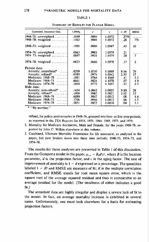
refund, for policy anniversaries in 1948-76, grouped into four- or five-year periods, as reported in the TSA Reports for 1954, 1959, 1964, 1969, 1973, and 1979.

2. Mortality for Medicare Recipients, Male and Female, for the years 1968-78, re- ported by John C. Wilkin elsewhere in this volume.

3. Combined, Ultimate Mortality Experience for life insurance, as analyzed in the paper, but now broken down into three time periods: 1948-53, 1954-73, and 1974-78.

The results for these analyses are p resen ted in Table 1 of this discussion.

F rom the Gom per t z model in the paper, tx~,s = Bodsc y, where B is the location

parameter , d is the project ion factor, and c is the aging factor. The rate of

improvement of mortal i ty is 1 - d expressed as a percentage. The quantit ies

labeled I - R 2 and R M S E are measures of fit; R is the multiple correlat ion

coefficient, and R M S E stands for root mean square error, which is the

square root o f the average squared residual and thus is comparable to an

average residual for the model . (The smallness of ei ther indicates a good

fit.)

The annui tant data are highly irregular and display a severe lack of fit to

the model. In fact , an average mortality increase is exhibi ted in several

cases . Unfor tunate ly , one must look e lsewhere for a basis for estimating

project ion factors .

DISCUSSION 179

The medicare data provide such a basis, for ages 65-90, since they are homogeneous, complete, and accurate. For 1968-78, uniform, average, an- nual improvement factors are exhibited as 1.5 percent for males and 2.4 percent for females. The fits for the medicare data are the best found. A similar figure for 1948-78 using the insurance data exhibits 1.2 percent, which is predominantly male mortality.

Splitting the data into before and after 1974 shows an increase of 2.2 percent, to a 3.4 percent rate of improvement for the insurance data; no change for males receiving medicare; and an increase of 0.1 percent for like females. With essentially no change in the rate of improvement in recent years for medicare, the significant change from a 1.2 percent to a 3.4 percent rate of improvement in the insurance might be questioned. Perhaps it is due to some factor other than pure mortality.

It is interesting to note that the values for c differ among the three groups but have not changed within the groups since 1954.

Photocopies of the tables of residuals for the analyses cited above are available from the author.