PARAMETRIC LEVEL SET METHODS FOR INVERSE PROBLEMS

ALIREZA AGHASI, MISHA KILMER, ERIC L. MILLERAAGHAS01@ECE.TUFTS.EDU, MISHA.KILMER@TUFTS.EDU, ELMILLER@ECE.TUTS.EDU

Abstract. In this paper, a parametric level set method for reconstruction of obstacles in gen-eral inverse problems is considered. General evolution equations for the reconstruction of unknownobstacles are derived in terms of the underlying level set parameters. We show that using theappropriate form of parameterizing the level set function results a significantly lower dimensionalproblem, which bypasses many difficulties with traditional level set methods, such as regularization,re-initialization and use of signed distance function. Moreover, we show that from a computationalpoint of view, low order representation of the problem paves the path for easier use of Newton andquasi-Newton methods. Specifically for the purposes of this paper, we parameterize the level setfunction in terms of adaptive compactly supported radial basis functions, which used in the pro-posed manner provides flexibility in presenting a larger class of shapes with fewer terms. Also theyprovide a “narrow-banding” advantage which can further reduce the number of active unknowns ateach step of the evolution. The performance of the proposed approach is examined in three examplesof inverse problems, i.e., electrical resistance tomography, X-ray computed tomography and diffuseoptical tomography.

Key words. parametric level set methods, shape-based methods, inverse problems

1. Introduction. Inverse problems arise in many applications of science and en-gineering including e.g., geophysics [66,84], medical imaging [3,48,79], nondestructiveevaluation [47, 49] and hydrology [13, 70, 81]. In all cases the fundamental problemis usually extracting the information concerning the internal structure of a mediumbased on indirect observations collected at the periphery, where the data and theunknown are linked via a physical model of the sensing modality. A fundamentalchallenge associated with many inverse problems is ill-posedness (or ill-conditioningin the discrete case), meaning that the solution to the problem is highly sensitiveto noise in the data or effects not captured by the physical model of the sensor.This difficulty may arise due to the underlying physics of the sensing system whichin many cases (e.g., electrical impedance tomography [17], diffuse optical tomogra-phy [3], inverse scattering [24], etc) causes the data to be inherently insensitive tofine scale variations in the medium. This phenomenon makes such characteristicsdifficult, if not impossible to recover stably [73]. Another important factor causingthe ill-posedness is limitations in the distribution of the sensors yielding sparse datasets that again do not support the recovery of fine scale information uniformly in theregion of interest [52]. Many inverse problems of practical interest in fact suffer fromboth of these problems. From a practical point of view, left untreated, ill-posednessyields reconstructions contaminated by high frequency, large amplitude artifacts.

Coping with the ill-posedness is usually addressed through the use of regular-ization [27, 53]. Based on prior information about the unknowns, the regularizationschemes add constraints to the inverse problem to stabilize the reconstructions. Whenthe inverse problem is cast in a variational framework, these regularization methodsoften take the form of additive terms within the associated cost function and are inter-preted as penalties associated with undesirable characteristics of the reconstruction.They may appear in various forms such as imposing boundedness on the values ofthe unknown quantity (e.g., Tikhonov or minimum norm regularizations [30, 73]) orpenalizing the complexity by adding smoothness terms (e.g., the total variation reg-ularization [1]). These regularization schemes are employed in cases where one seeksto use the data to determine values for a collection of unknowns associated with adense discretization of the medium (e.g, pixels, voxels, coefficients in a finite element

1

representation of the unknown [62]).

For many problems, the fundamental objective of the process is the identificationand characterization of regions of interest in a medium (tumors in the body [12],contaminant pools in the earth [34], cracks in a material sample [69], etc). For suchproblems, an alternative to forming an image and then post-processing to identifythe region is to use the data to directly estimate the geometry of the regions as wellas the contrast of the unknown in these regions. Problems tackled in this way areknown as the inverse obstacle or shape-based problems. For earlier works in thisarea see [18, 40, 43] and particularly the more theoretical efforts by Kirsch [39] andKress et al. [41]. Such processes usually involve a rather simple parametrization ofthe shape and perform the inversion based on using the domain derivatives mappingthe scattering obstacle to the observation. Relative to pixel-type approaches, thesegeometric formulations tend to result in better posed problems due to a more ap-propriate obstacle representation. Moreover, in such problems the regularization canbe either performed implicitly through the parametrization or expressed in terms ofgeometric constraints on the shape [44]. However, this class of shape representationis not topologically flexible and the number of components for the shape should bea priori known [63]. They also create difficulties in encountering holes and high cur-vature regions such as the corners. These difficulties have lead over the past decadeor so to the development of shape-based inverse methods employing level set-typerepresentation of the unknowns.

The concept of level sets was first introduced by Osher and Sethian in [57]. Thismethod was initially designed for tracking the motion of a front whose speed dependson the local curvature. The application of the level set approach to inverse problemsinvolving obstacles was discussed by Santosa in [63]. One of the most attractivefeatures of the level set method is its ability to track the motion through topologicalchanges. More specifically, an a priori assumption about the connectedness of theshapes of interest was no longer required. Following Santosa’s work, Litman et al.in [46] explored the reconstruction of the cross-sectional contour of a cylindrical target.Two key distinguishing points about this work were in the way that the authors dealtwith the deformation of the contour, and in their use of the level set method torepresent the contour. The shape deformation method implemented in this work wasenabled by a velocity term, and lead to a closed-form derivative of the cost functionalwith respect to a perturbation of the geometry. They defined shape optimization asfinding a geometry that minimizes the error in the data fit. Later Dorn et al. in [26]introduced a two-step shape reconstruction method that was based on the adjoint fieldand level set methods. The first step of this algorithm was used as an initializationstep for the second step and was mainly designed to deal with the non-linearitiespresent in the model. The second step of this algorithm used a combination of thelevel set and the adjoint field methods. Although inspired by the works of [46,57,63],the level set method used by Dorn et al. was not based on a Hamilton-Jacobi typeequation, instead, an optimization approach was employed, and an inversion routinewas applied for solving the optimization. The level set ideas in inverse problemswere further developed to tackle more advanced problems such as having shapes withtextures or multiple possible phases [15,25]. Moreover, regarding the evolution of thelevel set function where usually gradient descent methods are the main minimizationschemes applied, some authors such as Burger [10] and Soleimani [67] proposed usingsecond order convergent methods such as the Newton and quasi-Newton methods.

Although level set methods provide large degrees of flexibility in shape represen-

2

tation, there are numerical concerns associated with these methods. Gradient descentmethods used in these problems usually require a long evolution process. Althoughthis problem may be overcome using second order methods, the performance of thesemethods for large problems such as 3D shape reconstructions remains limited andusually gradient descent type methods are the only option for such problems. More-over re-initialization of the level set function to keep it well behaved and velocityfield extensions to globally update the level set function through the evolution areusually inevitable and add extra computational costs and complexity to the prob-lem [56]. More detailed reviews of level set methods in inverse problems can be foundin [11,24].

In all traditional level set methods already stated, the unknown level set functionbelongs to an infinite dimensional function space. From an implementation perspec-tive, this requires the discretization of the level set function onto a dense collectionof nodes. An alternative to this approach is to consider a finite dimensional functionspace or a parametric form for the level set function such as the space spanned bya set of basis functions. Initially, Kilmer et al. in [38] proposed using a polynomialbasis for this purpose in diffuse optical tomography applications. In this approach,the level set function is expressed in terms of a fixed order polynomial and evolvedthrough updating the polynomial coefficients at every iteration. Parametrization ofthe level set function later motivated some authors in field of mechanics to use it inapplications such as structural topology optimization [60, 77, 78]. One of the maincontributions in this regard is the work by Wang et al. in [78]. Here the level setfunction is spanned by multiquadric radial basis functions as a typical basis set inscattered data fitting and interpolation applications. Authors showed that throughthis representation, the Hamilton-Jacobi partial differential equation changes into asystem of ordinary differential equations and the updates for the expansion coefficientsmay be obtained by numerically solving an interpolation problem at every iteration.

More recently, the idea of parametric representation of the level set functionhas been considered for image processing applications [5, 29]. Gelas et al. in [29]used a similar approach as the one by Wang et al. for image segmentation. Asthe basis set they used compactly supported radial basis functions, which not onlyreduce the dimensionality of the problem due to the parametric representation, butalso reduce the computation cost through the sparsity that this class of functionsprovide. As advantages of the method they showed that appropriate constraints onthe underlying parameters can avoid implementation of the usual re-initialization.Also the smoothness of the solution is guaranteed through the intrinsic smoothnessof the underlying basis functions, and in practice no further geometric constraintsneed to be added to the cost function. As an alternative to this approach, Bernardet al. in [5] parameterized the level set function in terms of B-splines. One of themain advantages of their method was representing the the cost function minimizationdirectly in terms of the B-spline coefficients and avoiding the evolution through theHamilton-Jacobi equation.

In this paper the general parametric level set approach for inverse problems isconsidered. For an arbitrary parametrization of the level set function, the evolutionequation is derived in terms of the underlying parameters. Since one of the mainadvantages of this approach is low order representation of the level set function, inpractice the number of unknown parameters in the problem is much less than thenumber of pixels (voxels) in a traditional Hamilton-Jacobi type of level set method,therefore we concentrate on faster converging optimization methods such as the New-

3

ton or quasi-Newton type method. To represent the parametric level set function, asin [29, 78] we have proposed using radial basis functions. However unlike the previ-ous works employing radial basis functions in a level set framework, in addition tothe weighting coefficients, the representation is adaptive with respect to the centersand the scaling of the underlying radial basis functions. This technique basically pre-vents using a large number of basis terms in case that no prior information about theshape is available. To fully benefit from this adaptivity, we further narrow our choiceby considering compactly supported radial basis functions. Apparently, this choicewould result sparsity in the resulting matrices. However, we will discuss a behavior ofthese functions which can be exploited to further reduce the number of underlying ba-sis terms and provide the potential to reconstruct rather high curvature regions. Theflexibility and performance of proposed methods will be examined through illustrativeexamples.

The paper is structured as follows. In Section 2 we review shape-based inverseproblems in a general variational framework. Section 3 is concerned with obtainingthe first and second order sensitivities of the cost function with respect to the func-tions defining the shape. Based on the details provided, a brief revision of the relevanttraditional level set methods is provided paving the path to use parametric level setmethods. In Section 4 the general parametric level set method will be introducedand evolution equations corresponding to the underlying parameters are derived. InSection 5 an adaptive parametric level set based on the radial basis functions willbe proposed and the approach will be narrowed down to compactly supported classof functions, due to their interesting properties. Section 6 will examine the methodthrough some examples in the context of electrical resistance tomography, X-ray to-mography and diffuse optical tomography. Finally in Section 7 some concluding re-marks and suggestions will be provided.

2. Problem Formulation.

2.1. Forward Modelling. The approach to modelling and determination ofshape we consider in this paper is rather general with the capability of being appliedto a range of inverse problems. In Section 6 we specifically consider three applications:electrical resistance tomography, limited view X ray tomography, and diffuse opticaltomography. The details of the specific problems will be provided in the same sectionwithin the context of the examples themselves. Up until that point, we have chosento keep the discussion general.

Consider Ω to be a compact domain in Rn, n ≥ 2, with Lipschitz boundary ∂Ω.

Further assume for x ∈ Ω, a space dependent property p(x) ∈ Sp, where Sp is aHilbert space. A physical model M acts on a property of the medium (e.g., electricalconductivity, mass density or optical absorption), p, to generate an observation (ormeasurement) vector u,

u = M(p), (2.1)

where u itself belongs to some Hilbert space Su. In most applications u is a vector inC

k, the space of k dimensional complex numbers where k represents the number ofmeasurements and accordingly a canonical inner product is used.

As a convention throughout this paper, to keep the generality of notation, theinner products and norms corresponding to any Hilbert space H, are subindexed withthe notation of the space itself, e.g. ⟨., .⟩H.

4

2.2. Inverse Problem. The goal of an inverse problem is the recovery of in-formation about the property p based on the data u. Here we consider a variationalapproach where the estimate of p is generated as the solution to an optimization prob-lem. The functional underlying the problem is usually comprised of two terms. Thefirst term demands that the estimate of p be consistent with the data in a mathe-matically precise sense. As is well known however, many interesting inverse problemsare quite ill-posed. This means when the data consistency is our only concern, theresulting estimate of p could be quite far from the truth, corrupted by artifacts suchas high frequency and large amplitude oscillations. Hence, an additional term (orterms) are required in the formulation of the variation problem which capture ourprior knowledge concerning the expected behavior of the p in Ω. Such terms serve tostabilize (or regularize) the inverse problem. Defining a residual operator as

R(p) = M(p) − u, (2.2)

the inverse problem is formulated in the following manner

minp

F (p) = 1

2∥R(p)∥2Su + L(p), (2.3)

where L is the regularization functional. Appropriate choice of L is usually basedon properties of the problem. In the typical case where the unknown property p isrepresented as a dense collection of pixels (or voxels) in Ω, the regularization penal-ties are used to enforce smoothness and boundedness of p in Ω. These are usuallyconsidered in the framework of Tikhonov and total variation regularizations [1, 73].An alternative approach that has been of great interest in recent years is based ongeometric parameterizations of the unknown. Here the regularization penalties areeither embedded in the nature of the unknown or expressed as geometric constraintson the unknown. No matter which approach is used, usually in defining L differentspaces and their corresponding norms may be used. For a more detailed review ofsuch methods an interested reader is referred to [24,76]. However, since the idea to bepresented in this paper focuses on appropriately reducing the dimensionality of theinverse problem and as will be examined through various examples the problem showsto be well-posed enough that no necessary regularization terms need to be added tothe cost function, L will be neglected in our future discussions of F .

2.3. A Shape-Based Approach For the Unknown Parameter. For a largeclass of “shape-based” inverse problems [24, 42, 51, 63], it is natural to view p(x) asbeing comprised of two classes, i.e., foreground and background. The problem thenamounts to determination of the boundary separating these classes as well as charac-teristics of the property values in each class. In the simplest case, p(x) is piecewiseconstant while in more sophisticated cases p(x) may be random and characterized bydifferent probabilistic models in the two regions. In this paper, we assume that overeach region p(x) is at least differentiable. The property of interest in this case is usu-ally formulated through the use of a characteristic function. Given a closed domainD ⊆ Ω with corresponding boundary ∂D, the characteristic function χD is defined as

χD(x) = { 1 x ∈D0 x ∈ Ω ∖D. (2.4)

Accordingly, the unknown property p(x) can be defined over the entire domain Ω as

p(x) = pi(x)χD(x) + po(x)(1 − χD(x)). (2.5)

5

Unlike p(x) which is clearly not differentiable along ∂D, pi(x) indicating the propertyvalues inside D and po(x) denoting the values outside, are assumed to be smoothfunctions, and as mentioned earlier, at least belonging to C1(Ω).

In a shape-based approach, finding ∂D is a major objective. As (2.5) and (2.4)show, p(x) is implicitly related to D and to find ∂D, a more explicit way of relatingthem should be considered. In this regard the idea of using a level set function provesto be especially useful [63]. Here ∂D is represented as some level set of a Lipschitzcontinuous function φ ∶ Ω → R. When the zero level set is considered, φ(x) is relatedto D and ∂D via

⎧⎪⎪⎪⎨⎪⎪⎪⎩φ(x) > 0 ∀x ∈Dφ(x) = 0 ∀x ∈ ∂Dφ(x) < 0 ∀x ∈ Ω ∖D. (2.6)

Making the use of a Heaviside function, defined as H(.) = 12(1+ sign(.)), the function

p(x) can be represented as

p(x) = pi(x)H(φ(x)) + po(x)(1 −H(φ(x))). (2.7)

This equation in fact maps the space of unknown regions D into the space of unknownsmooth functions φ.

3. Inversion as a Cost Function Minimization. In this section we developthe mathematical details of the minimization problem (2.3) when a shape-based ap-proach as (2.7) is considered. Most current methods use the first and second ordersensitivities of the cost function with respect to the unknown parameter to performthe minimization [11]. Based on the general details provided, we will briefly revisitthe traditional level set approaches relevant to this paper in Section 3.2, since under-standing the details better justifies the use of parametric level set methods.

3.1. Cost Function Variations Due to the Unknowns. We begin by as-suming that the first and second order Frechet derivatives of R(p) exist and denotethem as R′(p)[ . ] and R′′(p)[., .]. The first order Frechet derivative of a function (ifit exists) is a bounded and linear operator. The second order Frechet derivative isalso bounded but bilinear, which means the operator acts on two arguments and islinear with respect to each [4].

For an arbitrary variation δp ∈ Sp and the real scalar ε, using the generalizedTaylor expansion we have

R(p + εδp) = R(p) + εR′(p)[δp] + ε22R′′(p)[δp, δp] +O(ε3). (3.1)

Rewriting F (p) as

F (p) = 1

2⟨R(p),R(p)⟩Su , (3.2)

and recalling the fact that ⟨u1, u2⟩Su = ⟨u2, u1⟩Su for u1, u2 ∈ Su and overline denotingcomplex conjugate, the variations of the cost function with respect to the variationsof p can be derived as

F (p + εδp) = F (p) + εF ′(p)[δp] + ε22

F ′′(p)[δp, δp] +O(ε3), (3.3)

6

where for p1, p2 ∈ SpF ′(p)[p1] = Re⟨R′(p)[p1],R(p)⟩Su (3.4)

and

F ′′(p)[p1, p2] = Re⟨R′(p)[p1],R′(p)[p2]⟩Su + Re⟨R′′(p)[p1, p2],R(p)⟩Su . (3.5)

The notation Re indicates the real part of the corresponding quantity. DenotingR′(p)∗[ . ] as the adjoint operator between Su and Sp as

⟨u,R′(p)[p]⟩Su = ⟨R′(p)∗[u], p⟩Sp , ∀u ∈ Su,∀p ∈ Sp, (3.6)

(3.4) can be written as

F ′(p)[p1] = Re⟨R′(p)∗[R(p)], p1⟩Sp . (3.7)

Equations (3.4), (3.7) and (3.5) are in fact the first and second order Frechet deriva-tives of F with respect to p. In a more general context (and indeed one which we shalluse in Section 4), p itself can be the map over some variable v from another Hilbertspace Sv into Sp, i.e., p(v) ∶ Sv → Sp. Assuming the existence of the first and secondorder Frechet derivatives of p with respect to v, denoted as p′(v)[ . ] and p′′(v)[., .],the first and second order Frechet derivatives of F with respect to v can be obtainedusing the chain rule as

F ′(v)[v1] = F ′(p)[p′(v)[v1]] (3.8)

and

F ′′(v)[v1, v2] = F ′′(p)[p′(v)[v1], p′(v)[v2]] + F ′(p)[p′′(v)[v1, v2]], (3.9)

where v1, v2 ∈ Sv. Equations (3.8) and (3.9) themselves can be easily expressed interms of R(p) and its derivatives using (3.4) and (3.5). These equations will beused later as the key equations in finding the sensitivities in our parametric level setrepresentation of p.

3.2. Pixel Based Minimizations (Revisiting Traditional Level Set Meth-ods). In the specific context of the shape-based inverse problems of interest here, thefirst and second order sensitivities of the cost function F with respect to the functionsdefining p(x) in (2.7) i.e., φ(x), pi(x) and po(x), can be used to form a minimiza-tion process. Based on the order of the sensitivities available, first order optimizationmethods such as gradient descent or second order methods such as Newton or quasi-Newton techniques can be implemented.

For simplicity in reviewing the current methods, we assume that pi and po areknown a priori and only the shape (i.e., the zero level set of φ) is unknown (see[25,28,75] for details on the recovery of both the shape as well as the contrast function).In an evolution approach it is desired to initialize a minimization process with somelevel set function φ0 and evolve the function to find a φ which minimizes F . To takeinto account the concept of evolution, an artificial time is defined where the level setfunction at every time frame t ≥ 0 is rewritten as φ(x; t) and the zero level set ofφ(x; t) is denoted as ∂Dt. A straightforward differentiation of φ(x; t) = 0 with respectto t yields to the Hamilton-Jacobi type equation

∂φ

∂t+ V (x; t) ⋅ ∇φ = 0 (3.10)

7

for the points on ∂Dt where V (x; t) = dx/dt. To move the interface in the normaldirection, V (x; t) should be chosen as v(x; t)n(x; t) where v is a scalar speed functionand n = ∇φ/∣∇φ∣ is the unit outward vector on ∂Dt. Incorporating this into theminimization of F , the speed function for the points on ∂Dt, denoted as v, can bechosen to be in the steepest descent direction of F which is [24]

v = −Re{(po − pi)R′(p)∗ [R(p)]}. (3.11)

As (3.11) is only valid for x ∈ ∂D, a velocity extension should be performed to extend vto v defined over the entire domain Ω and therefore capable of globally evolve the levelset function [56]. Beside this classical level set approach, other ways of representingthe speed functions and performing the minimization process are proposed [10,50,58].For example, Hadj Miled and Miller [50] proposed a normalized version of the classicspeed function in the context of electrical resistance tomography.

Some authors have also proposed using Newton type methods to update v atevery iteration (e.g., see [10,63,68]). Analogous to (2.2) and (3.2), in these problemsthe residual operator and the cost function are usually written directly as R(D) andF (D), functions of the shape itself. Assuming the existence of the first and secondorder shape derivatives [55], denoted as F ′(D)[ . ] and F ′′(D)[., .], at every timestep the Newton update v is obtained by solving [11]

F ′′(D)[w, v] + F ′(D)[w] = 0 ∀w ∈ SD. (3.12)

Here SD is an appropriate Hilbert space such as L2(∂D), which may depend on thecurrent shape [9, 10]. Considering the general forms of the derivatives as (3.4) and(3.5), in a Gauss-Newton method the second derivatives of R are disregarded and(3.12) becomes

Re⟨R′(D)[v],R′(D)[w]⟩Su + Re⟨R′(D)[w],R(D)⟩Su = 0 ∀w ∈ SD. (3.13)

Furthermore, to avoid ill conditioning, in a Levenberg-Marquardt approach (3.13) isregularized as

Re⟨R′(D)[v],R′(D)[w]⟩Su + Re⟨R′(D)[w],R(D)⟩Su + λ⟨v, w⟩SD = 0 ∀w ∈ SD.(3.14)

in which for λ > 0, the equation is shown to be well-posed [10]. Similar to theprevious approach, once v is obtained, a velocity extension is performed to result aglobally defined v which can be used to update φ. However, although using secondorder methods can reduce the number of iterations in finding a minima, compared togradient descent methods, they do not necessarily reduce the computation load.

From an implementation perspective there are some concerns using the afore-mentioned methods. The gradient descent method usually requires many iterationsto converge and performances become poor for low sensitivity problems [50]. Althoughusing Newton and quasi-Newton methods to update the level set function increases theconvergence rate, they are usually computationally challenging and for large problemsand relatively finer grids, a large system of equations must be solved at every iteration.Also for both types of methods, there are usually added complications of the level setfunction re-initialization and speed function extension. The approach that we will putforth in the next section is capable of addressing these problems. It is low order andnumerically speaking, the number of unknowns involved in the problem are usuallymuch less than the number of grid points and hence allows us to easily use second

8

order methods. Moreover, our proposed method does not require re-initialization ofthe level set function, speed function extension or even length-type regularization asa common regularization in many shape-based methods (e.g., see [24,33,50]) and ourlevel set function remains well behaved through the corresponding evolution process.

4. A Parametric Level Set Approach. As discussed earlier, in most currentshape-based methods φ(x) is represented by function values on a dense discretizationof x-space as part of a discretization of the underlying evolution equation or Newton-type algorithm. Consider now the level set function to be still a function of x butalso a function of a parameter vector μ = (μ1, μ2,⋯, μm) ∈ Rm. In this case we definethe continuous Lipschitz function φ ∶ Ω × R

m → R, as a parametric level set (PaLS)representation of D if for a c ∈ R

⎧⎪⎪⎪⎨⎪⎪⎪⎩φ(x,μ) > c ∀x ∈Dφ(x,μ) = c ∀x ∈ ∂Dφ(x,μ) < c ∀x ∈ Ω ∖D. (4.1)

In the PaLS approach we assume that the general form of φ(x,μ) is known and thespecification of μ can explicitly define the level set function over the entire domain Ω.In other words the evolution of φ required to solve the underlying inverse problems isperformed via the evolution of μ. An example of a PaLS function is a basis expansionwith known basis functions and unknown weights and as will be shown later in thispaper we considerably expand on this notion. We call μ the PaLS parameters.

To setup the problem using the PaLS approach, consider momentarily that pi(x)and po(x) are known a priori (later we will appropriately take away this restriction).Based on (4.1) p is written as

p(x,μ) = pi(x)H(φ(x,μ) − c) + po(x)(1 −H(φ(x,μ) − c)). (4.2)

Under this model, we now view F in (3.2) as a function of μ, i.e. F (μ) ∶ Rm → R.Therefore unlike the classic level set approach, the unknown is no longer the functionφ, but a vector belonging to R

m, where m is usually much smaller than the number ofunknowns associated with a discretization of x-space. With this model and assuming(1) φ is sufficiently smooth with respect to the elements of μ and (2) the discontinuousHeaviside function is replaced by a C2 approximation (e.g., [83]) denoted as Hrg, wenow proceed to formulate a second order approach for the minimization of F (μ). Tobegin, rewriting (4.2) with Hrg and taking a derivative with respect to φ yields

∂p

∂φ= (pi − po)δrg(φ − c), (4.3)

where δrg(.) is accordingly the regularized version of the Dirac delta function (seeexamples in [72,83]). Using the chain rule gives

∂p

∂μj= ∂p

∂φ

∂φ

∂μj= (pi − po)δrg(φ − c) ∂φ

∂μj. (4.4)

9

Now using (4.4) with (3.8) and (3.7), the gradient vector for F is

∂F

∂μj= F ′(p)[ ∂p

∂μj]

= Re⟨R(p),R′(p)[ ∂p∂μj

]⟩Su (4.5)

= Re⟨R′(p)∗[R(p)], (pi − po)δrg(φ − c) ∂φ∂μj

⟩Sp . (4.6)

We denote by Jµ(F ) the gradient of F with respect to the parameter vector μ. Withthis notation a gradient descent equation can be formed to evolve the PaLS functionas

μ(t+1) = μ(t) − λ(t)Jµ(F )∣µ=µ(t)

t ≥ 0, (4.7)

where λ(t) > 0 is the iteration step [6]) and (4.7) is assumed to be initialized withsome μ(0). Although gradient decent is relatively simple to implement, it is knownto be slow to converge and can suffer from difficulties associated with scaling of theparameters [21]. Moreover, the use of gradient decent fails to take advantage of oneof the primary benefits of the PaLS idea; namely the ability to specify a level setfunction using a small (relative to a discretization of x-space) number of parameters.Under this model, it becomes feasible and indeed useful to consider higher orderoptimization methods (Newton or quasi-Newton) for the determination of μ. Thesemethods usually use the information in the Hessian, which we now derive. To calculatethe elements of the Hessian matrix for F using (4.4) we have

∂2p

∂μj∂μk= (pi − po)(δrg(φ − c) ∂2φ

∂μj∂μk+ δ′rg(φ − c) ∂φ

∂μj

∂φ

∂μk

), (4.8)

where δ′rg(.) is the derivative of the regularized Dirac delta function. Based on (3.9)and (3.5) we have

∂2F

∂μj∂μk= F ′′(p)[ ∂p

∂μj,∂p

∂μk

] + F ′(p)[ ∂2p

∂μj∂μk

]= Re⟨R′(p)[ ∂p

∂μj],R′(p)[ ∂p

∂μk]⟩Su + Re⟨R′′(p)[ ∂p

∂μj,∂p

∂μk],R(p)⟩Su

+ Re⟨R′(p)∗[R(p)], ∂2F

∂μj∂μk⟩Sp . (4.9)

This equation is in fact the exact expression for the elements of the Hessian matrixfor F . However as mentioned earlier, in methods such as the Gauss-Newton orLevenberg-Marquardt, to reduce the computation cost the Hessian is approximatedin that the terms containing second order derivatives are disregarded. Following thatapproach here, (4.9) becomes

∂2F

∂μj∂μk≃ Re⟨R′(p)[ ∂p

∂μj],R′(p)[ ∂p

∂μk]⟩Su (4.10)

= Re⟨R′(p)[(pi − po)δrg(φ − c) ∂φ∂μj

],R′(p)[(pi − po)δrg(φ − c) ∂φ∂μk

]⟩Su .(4.11)

10

We denote as Hµ(F ) the approximate Hessian matrix, the elements of which areobtained through (4.10). Having this in hand, a stable and faster converging PaLSfunction evolution can be proposed by solving the following Levenberg-Marquardtequation for μ(t+1)

[Hµ(F )∣µ=µ(t)

+ λ(t)I](μ(t+1) −μ(t)) = −Jµ(F )∣µ=µ(t)

t ≥ 0. (4.12)

Here λ(t) is a small positive number chosen at every iteration and I is the identitymatrix. In fact referring to (4.10) we can see that the approximate Hessian matrixHµ(F ) is a Gramian matrix and hence positive semidefinite. Therefore adding thesmall regularization term λ(t)I would make the matrix at the left side always positivedefinite and hence the system of equations resulting the updates for μ always has aunique solution. The left hand side matrix being strictly positive definite guaranteesΔμ(t) = μ(t+1) −μ(t) to be in the descent direction since we have

[Δμ(t)]T[Jµ(F )] = −[Δμ(t)]T[Hµ(F ) + λ(t)I][Δμ(t)] < 0 (4.13)

where the superscript T denotes the matrix transpose. More technical details aboutthe implementation of the Levenberg-Marquardt algorithm such as the techniques ofchoosing λ(t) at each iteration based on trust region algorithms are available in [6,21].

We now turn our attention to the determination of pi(x) and po(x). For simplicityhere we assume that p(x) is piecewise constant as is often the case in work of thistype [71]. This, in addition to the shape parameters, we need to determine twoconstants defining the contrasts over the regions. We do note that the approachcan easily be extended to consider other low order “texture models” as is done ine.g. [37]. As our primary interest in this paper is a new method for representingshape, we defer this work to the future. Under our piecewise constant contrast model,we denote the contrasts as pi(x) = pi and po(x) = po, were pi and po are unknownconstant values. Following analogous equations as (4.5) and (4.9), these parameterscan also be appended to the unknown PaLS parameters. The sensitivity of F withrespect to these parameters can also be derived based on the fact that

∂p

∂pi= 1 − ∂p

∂po=Hrg(φ − c). (4.14)

and the second order derivatives of p with respect to pi and po are zero.For the PaLS approach represented in this section, the intention is to keep the

formulations general and emphasize the fact that this representation can formally re-duce the dimensionality of the shaped based inversion. Clearly the expression ∂φ/∂μj

depends on how the PaLS functions are related to their parameters. In the next sec-tion a specific PaLS representation is presented the efficiency of which will be laterexamined through some examples.

5. PaLS Function Representation.

5.1. Adaptive Radial Basis Functions. As pointed out earlier, appropriatechoice of a PaLS function can significantly reduce the dimensionality of an inverseproblem. In this paper we are interested in a low order model for the level set func-tion which will provide flexibility in terms of its ability to represent shapes of varyingdegree of complexity as measured specifically by the curvature of the boundary. Thisrepresentation may allow for “coarse scale” elements capable of representing bound-aries of low curvature with few elements. Furthermore, it is desired to have finer

11

grain elements capable of capturing higher curvature portions of the boundary suchas sharp turns or corners. Such adaptability is desirable for a general PaLS represen-tation since the characteristics must be present for well-posed inverse problems suchas full view X-ray CT or even image segmentation where high fidelity reconstructionsare possible. On the other hand, as we demonstrate in Section 6, for severely ill-posedproblems, the availability of models with this parsimonious, but flexible structure mayallow for the recovery of geometric detail that otherwise would be not be obtainableform e.g., a traditional level set or pixel based approach. Writing a PaLS functionas a weighted summation of some basis functions may be a reasonable choice here,where different terms in the summation may handle some desired properties aboutthe shape. Here we focus specifically on the class of radial basis functions (RBF).We are motivated to concentrate on RBFs as they have shown to be very flexible inrepresenting functions of various detail levels. This flexibility makes them appropriatechoice for topology optimization [78], solving partial differential equations [36] andmultivariate interpolation of scattered data [32,80]. Some examples of commonly usedRBFs are Gaussian, multiquadric, polyharmonic splines and thin plate splines. Moredetails about these functions and their properties are available in [8].

Based on the statements made, consider the PaLS function

φ(x,α) = m0∑j=1

αjψ(∥x −χj∥) (5.1)

where ψ ∶ R+ → R is a sufficiently smooth radial basis function, α ∈ Rm0 is the PaLSparameter vector and ∥.∥ denotes the Euclidean norm. The points χj are called theRBF centers. In an interpolation context, usually the centers are decided in advanceand distributed more densely in regions with more data fluctuations. However, ina PaLS approach there may be limited information about the shape geometry andtherefore more flexibility is required. Thus here we consider a more general PaLSfunction of the form

φ(x, [α,β,χ]) = m0∑j=1

αjψ(∥βj(x −χj)∥†), (5.2)

for which the vector of centers χ = [χ1,χ2,⋯,χm0] and the dilation factors β =[β1, β2,⋯, βm0

] are added to the set of PaLS parameters. Also in order to make thePaLS function globally differentiable with respect to the elements of β and χ, similarto [1] a smooth approximation of the Euclidean norm is used as

∥x∥† ∶= √∥x∥2 + υ2 ∀x ∈ Rn, (5.3)

where υ ≠ 0 is a small real number. The use of (5.2) rather than (5.1) makes thePaLS function capable of following more details through scaling the RBFs or floatingcenters moving to regions where more details are required. To incorporate this intothe optimization methods described, the sensitivities of φ with respect to the PaLSparameters are

∂φ

∂αj= ψ(∥βj(x −χj)∥†) (5.4)

and

∂φ

∂βj= αjβj

∥(x −χj)∥2∥βj(x −χj)∥†ψ′(∥βj(x −χj)∥†). (5.5)

12

Also considering χ(k)j and x(k) to be the kth components of χj and x as points in R

n,for k = 1,2,⋯, n we have

∂φ

∂χ(k)j

= αjβ2j

χ(k)j − x(k)

∥βj(x −χj)∥†ψ′(∥βj(x −χj)∥†). (5.6)

Clearly the sensitivities obtained are general and valid for any RBF in C1(R+). In thenext section, we consider a specific class of RBFs that we have found to be particularlywell suited to the PaLS problem.

5.2. The Choice of Compactly Supported Radial Basis Functions. Usu-ally the RBFs used in various applications involving function representations are C∞

functions with global support [8]. However a different class of RBFs which have re-cently been under consideration are the compactly supported radial basis functions(CSRBFs) [80]. These functions become exactly zero after a certain radius while stillretaining various orders of smoothness. From a numerical point of view, compactsupport of the RBFs yields sparsity in the resulting matrices arising in the implemen-tation of these methods and hence reduces the computation cost. This was recentlythe motivation to use these functions in simplifying level set methods [29]. Anotherinteresting property of these functions is their local sensitivities to the underlyingparameters [80]. In other words, when a function is expressed as a weighted sum ofCSRBFs, changing a term would not have a global effect on the function and onlylocally deforms it.

Beside aforementioned advantages of the CSRBFs, our interest in this class ofRBFs arises from their potential in reconstructing the shapes with a very small numberof terms in a PaLS representation as (5.2). Furthermore, as will be explained, thisrepresentation can involve shapes with corners and rather high curvature regions. Forψ ≥ 0 being a smooth CSRBF, lets denote every basis term in (5.2) as

ψj(x) = ψ(∥βj(x −χj)∥†) (5.7)

and call ψj a bump. Due to the compact support of these functions, for every twobumps ψj and ψk we can write

supp(ψj +ψk) = supp(ψj) ∪ supp(ψk). (5.8)

For a real valued function ϑ defined over Rn we define

Ic(ϑ) ∶= {x ∶ ϑ(x) ≥ c}. (5.9)

Clearly for c > 0, Ic(ϑ) represents the interior of the c-level set of ϑ. Based on (5.8)and the smoothness of the bumps, we obviously have that as c → 0+, Ic(ψj + ψk)would tend to Ic(ψj)⋃Ic(ψk). More generally for αj > 0, Ic(∑m0

j=1 αjψj) tendsto ⋃m0

j=1 Ic(ψj) as c → 0+. In other words, using positively weighted CSRBFs andconsidering some level sets very close to zero can imply reconstruction of the shapethrough the union of some floating balls of various radii. Moreover Ic(ψj − αkψk)would tend to Ic(ψj)∖Ic(ψk) as c → 0+ and αk → +∞. Therefore in this context,bumps with larger negative coefficients can yield holes or inflect the shape by excludingsome portions of it. We would consider the two aforementioned properties of theCSRBFs as a “pseudo-logical” behavior of these functions. This property can resultin rather high curvature geometries with a limited number of bumps. Besides high

13

−1 0 1

−1

0

1 α = 1 α = −1

α = −50

α = −10

−1 1−1

1

Fig. 5.1. (a) Left: A close to zero (c = 0.01) level set of the function ψ1 + αψ2 for variousvalues of α. The CSRBF used is the Wendland’s function ψ1,1 (cf. Table 5.1), the dilation factorsare β1 = β2 = 1 and the centers are taken as χ1 = (−

14,− 1

4) and χ2 = (

25, 25). (b) Center: A PaLS

function involved in representation of a square at a close to zero level set. Only 5 bumps are involved.(c) Right: The representation of the square

Table 5.1

Compactly supported RBFs of minimal degree where � = ⌊n/2⌋ + l + 1 and (1 − r)+ =max{0,1 − r}

Function Smoothness

ψn,1(r) = (1 − r)�+1+ (( + 1)r + 1) C2

ψn,2(r) = (1 − r)�+2+ (( 2 + 4 + 3)r2 + (3 + 6)r + 3) C4

ψn,3(r) = (1 − r)�+3+ (( 3 + 9 2 + 23 + 15)r3+ C6

(6 2 + 36 + 45)r2 + (15 + 45)r + 15)curvature regions, low curvature segments (e.g., an almost straight line in R

2 ora planar segment in R

3) can be formed by interaction of two identical bumps butwith opposite signs at their footprint intersections. Figure 5.1.a sheds more light onaforementioned facts, and shows the interaction of two bumps, which for instance canrepresent a crescent with two rather sharp corners (α = −50), or a contour with a lowcurvature segment (α = −1). As a second example, a representation of a square usingonly 5 bumps is depicted in Figures 5.1.b and 5.1.c.

The most commonly used CSRBFs are those called Wendland’s functions [80].The smoothness and the compact support provided by Wendland’s functions are ofinterest and hence we shall use them as the basis for our PaLS approach. Wendland’sfunctions follow the general form of

ψn,l(r) = { Pn,l(r) 0 ≤ r ≤ 10 r > 1

(5.10)

when representing an RBF in Rn, with Pn,l being a univariate polynomial of degree⌊n/2⌋ + 3l + 1. In terms of smoothness, this class of RBFs belong to C2l. A derivation

of these functions is provided in [80], from which we have listed the first few functionsin Table 5.1.

In the next section we discuss the regularized heaviside function and explainhow choosing an appropriate version of this function in (4.2), can pave the path forexploiting the pseudo-logical behavior of the bumps.

5.3. Numerical Approximation of the Heaviside Function. In a shape-based representation such as (4.2), solving the inverse problem numerically and mak-

14

0

0

0.1

0.4

0.6

0.8

1

ε−ε

H1,ε(x)

H2,ε(x)

x0

0

ε−εx

δ1,ε(x)

δ2,ε(x)

12ε

1ε

Fig. 5.2. (a) Left: Two regularized versions of the heaviside function. (b) Right: Correspondingregularized delta functions

ing the evolution of the level set function possible requires using a smooth version ofthe heaviside function. A possible C∞ regularization of H(.) denoted as H1,ε is theone used in [16], as

H1,ε(x) = 1

2(1 + 2

πarctan(πx

ε)). (5.11)

This function is commonly used in shape-based applications and specifically in therecent parametric representations of the level set function in image segmentation[5, 29]. Chan et al. in [14] have studied the characteristics of the resulting level setfunctions using H1,ε as the evolution proceeds. In the context of the current shape-based problem for which pi(x) = pi and po(x) = po, and considering the zero level set,(2.7) reveals that in an evolution process φ is likely to evolve towards a state thatH(φ(x)) = 1 for x ∈D and H(φ(x)) = 0 for x ∈ Ω ∖D. Referring to Figure 5.2.a, oneobserves that when H1,ε is used as the regularized heaviside function, in order to haveH1,ε(φ) ≃ 1 in D, the level set function should take rather large positive values (ascompared to ε) in this region. Analogously in Ω∖D, φ is pushed to take rather largenegative values. These constraints are implicitly imposed on the resulting level setfunction and specifically using CSRBFs in a PaLS approach as (5.2), the bumps areexpected to distribute throughout Ω to form a level set function which takes ratherlarge positive (or negative) values inside (or outside) D.

An alternative choice of the regularized Heaviside function is the C2 function,

H2,ε(x) =⎧⎪⎪⎪⎨⎪⎪⎪⎩

1 x > ε0 x < −ε

12+ x

2ε+ 1

2πsin(πx

ε) ∣x∣ ≤ ε, (5.12)

as proposed in [83]. It can be shown that if the nonzero level set c and ε are appro-priately set, using H2,ε enables us to exploit the pseudo-logical behavior describedpreviously. More specifically, for c > 0, and φ being a weighted sum of some bumps,and therefore compactly supported itself, we clearly want the points for which φ ≤ 0to belong to Ω ∖D, i.e., to correspond to the intensity po. Using (4.2), this requires

15

Fig. 5.3. (a) Left: A typical PaLS function resulted using H1,ε with 65 bumps and consideringthe zero level set. (b) Right: A typical PaLS function resulted using H2,ε with 30 bumps andconsidering the c level set

having H(φ−c) = 0 for φ ≤ 0. Referring to Figure 5.2.a, this condition is satisfied whenH2,ε is chosen as the regularized heaviside function and −c ≤ −ε (or in general case∣c∣ ≥ ε as the required criteria). Practically, this use of H2,ε takes away the implicitconstraint imposed on the level set function using H1,ε, i.e., the bumps do not haveto spread throughout Ω and may only concentrate inside and about the shape D toperform a higher resolution shaping. Figure 5.3 shows a typical shape representationresulted using H1,ε and H2,ε highlighting the pseudo-logical property.

Besides exploiting the pseudo-logical behavior, using H2,ε can provide anotheradvantage which reduces the dimensionality of the problem at every iteration, i.e., atevery step of the evolution process, the cost function will be sensitive to a specificgroup of PaLS parameters. To further describe this behavior, consider the termδrg(φ − c) ∂φ

∂μjappearing in both the Jacobian and the approximate Hessian of F in

(4.6) and (4.11). Also for an evolution iteration, assume the superscript (t) indicatingthe value of every quantity at that iteration. If for a PaLS parameter such as μj

0

δrg(φ(t) − c)∂φ(t)∂μj

0

∣μj

0=μ(t)j0

= 0 ∀x ∈ Ω, (5.13)

then using either one of the minimization schemes as (4.7) or (4.12) yields

μ(t+1)j0

= μ(t)j0. (5.14)

The reason for this result is clear for the gradient descent scheme (4.7), based on thefact that using (5.13) in (4.6) causes the jth

0element of gradient vector to vanish and

hence μ(t)j0

remaining unchanged at the corresponding iteration. For the Levenberg-

16

Marquardt scheme (4.12), using (5.13) in (4.11) causes all the elements in the jth0

row of the approximate Hessian matrix to vanish, which results the correspondingequation

λ(μ(t+1)j0

− μ(t)j0) = 0, (5.15)

again equivalent to (5.14). Therefore, for either one of the minimization schemes, if(5.13) holds, the PaLS parameter μj

0will stay unchanged in that iteration. We here

describe a common case that (5.13) holds during the evolution process:By using H2,ε as the regularized level set function, the corresponding regularized

delta function δ2,ε will be compactly supported (as shown in Figure 5.2.b), henceδ2,ε(φ − c) is only nonzero for c − ε < φ < c + ε. On the other hand, based on thePaLS approach presented in this paper using CSRBFs, for μj being any of the PaLS

parameters αj , βj or χ(k)j corresponding to the bump ψj , we have

supp( ∂φ∂μj

) ⊆ supp(ψj). (5.16)

This fact is easily observable in (5.4), (5.5) and (5.6), where the related derivativescan only have nonzero values in supp(ψj). Therefore, if at some iteration and for abump ψj

0,

supp (δ2,ε(φ − c)) ∩ supp(ψj0) = ∅, (5.17)

then in that iteration we have

δ2,ε(φ − c) ∂φ∂μj

0

= 0 (5.18)

and therefore the PaLS parameters corresponding to ψj0will stay unchanged in that

iteration. Figure 5.4 illustrates this phenomenon, showing a PaLS function composedof 6 bumps at some iterations. For 5 of the bumps used, the corresponding supportdoes intersect the region supp(δ2,ε(φ − c)), and therefore their corresponding param-eters have the potential to change at this state of the PaLS function. However, abump denoted as ψj

0, does not intersect supp (δ2,ε(φ − c)), and the underlying PaLS

parameters do not need to be considered in that iteration. This approach is similar tothe narrow-banding approach in traditional level-set methods [2,65], where the valuesof the level set function are only updated on a narrow band around the zero levelset and hence reducing the computation load. In our approach, however, this bandis the points for which c − ε < φ < c + ε and the bumps which do not intersect withthis band do not evolve at the corresponding iteration and hence their correspondingparameters are not updated.

In the next section, through a number of examples drawn from a wide range of ap-plications, we will show the superior performance of the proposed method specificallyexploiting the pseudo-logical behavior of the CSRBFs.

6. Examples. In this section, we examine our proposed method for three dif-ferent inverse problems, namely electrical resistance tomography, X-ray computedtomography and diffuse optical tomography. The examples are simulated for 2Dimaging and the results are provided in each section. Throughout all the examples,Ω denotes the region to be imaged and D denotes the shape domain as stated in theprevious sections.

17

−1 1−1

1

supp(∂φ

∂μj)

supp(∂φ

∂μj0

)

supp(δ2,ε(φ − c))

Fig. 5.4. (a) Left: A typical PaLS function composed of 6 bumps, and the c ± ε level sets.(b) Right: The bumps with active evolving parameters and the frozen bump

6.1. Electrical Resistance Tomography. As the first example we considerelectrical resistance tomography (ERT) categorized as a severely ill-posed problem [22,31]. The objective of this problem is the reconstruction of the electrical conductivitywithin a region of interest based on the potential or current measurements performedat the periphery of that region. Such reconstructions may be applicable in variousareas such as medical imaging [17], geophysics [23] and environmental monitoring [19].

For many geophysical applications the underlying physical model describing theDC potential u(x) inside Ω in terms of the conductivity σ(x) and the current sourcedistribution s(x) is

∇ ⋅ (σ(x)∇u(x)) = s(x) in Ω, (6.1)

σ∂u

∂ν= 0 on ∂Ωn ⊂ ∂Ω,

u = 0 on ∂Ωd = ∂Ω ∖ ∂Ωn,

where ν denotes the outward unit normal on ∂Ω and ∂Ωn and ∂Ωd correspond to Neu-mann and Dirichlet boundaries. In many of the applications (e.g., see [45, 54, 64, 74])the Dirichlet boundary condition is imposed as an approximation to the potential inregions far from the actual imaging region, and is used here for simplicity. For arbi-trary distributions of the conductivity, (6.1) is usually solved numerically by means offinite element or finite difference methods [68,82]. However, as the main focus of thepaper, we concentrate on piecewise constant conductivity distribution as σ(x) = σifor x ∈D and σ(x) = σo for x ∈ Ω ∖D.

For the inverse problem, the sensitivities of the measurements to perturbationsof the conductivity (in our approach the perturbations of the PaLS parameters) arerequired. For s(x) = δ(x − xs), i.e., a point source current at xs ∈ Ω, we denote byus(x) the resulting potential over the domain Ω and consider the measured potentialat xd ∈ Ω as

uds = ∫Ωus(x)δ(x − xd)dx. (6.2)

18

0

−0.2

−0.4

−0.6

−0.8

−1

−3−3 −0.5 −0.3 −0.1 0.1 0.3 0.5 3

y (m)

Ω

Ω′

u = 0u = 0

∂u

∂ν= 0

u = 0 x (m)

−

+

−

+

−

+

−

+−

+

−+

−

+

−

+−

+

−+

−

+

−

+−

+

−

+

−

+

−

+

−

+

−+

−

+

−

+

x

y

−0.5 −0.4 −0.3 −0.2 −0.1 0 0.1 0.2 0.3 0.4 0.5−1

−0.9

−0.8

−0.7

−0.6

−0.5

−0.4

−0.3

−0.2

−0.1

0

Fig. 6.1. (a) Left: The 2D modelling region for ERT. The darker interior region is the imagingregion surrounded by the sources and detectors. The dashed lines correspond to dipole nodes used inevery experiment (b) Right: The gray region shows the shape to be reconstructed in the ERT problem.The dots with “+” and “-” signs correspond to the centers of positive and negative weighted bumpsin the initial state of the problem. The black contour is the resulting c-level set of the initial PaLSfunction.

The variation of uds resulting from a perturbation δσ in the conductivity (i.e., theFrechet derivative of the measurements with respect to the conductivity) can be thenexpressed as [61,67]

dudsdσ

[δσ] = ∫Ωδσ ∇us ⋅ ∇ud dx, (6.3)

where ud is the adjoint field that results from placing the current point source atxd. To express the inverse problem in a PaLS framework, we consider M(.) asthe nonlinear forward model mapping the conductivity distribution into a vector ofvoltage measurements u obtained by performing M experiments, having a differentpoint source position at each experiment and making N� potential measurements for = 1,2,⋯,M . Having the residual operator R(σ) = M(σ) − u and using (6.3), theFrechet derivative denoted as R′(σ)[.] can be considered as a vector consisting of Msub-vectors R′�(σ)[.], structured as

R′�(σ)[δσ] = ⎛⎜⎝∫Ω δσ ∇u� ⋅ ∇u�1 dx⋮∫Ω δσ ∇u� ⋅ ∇u�N�

dx

⎞⎟⎠ . (6.4)

Here u� denotes the potential in the th experiment and u�i denotes the adjoint field

corresponding to the th experiment resulted from placing the current point source

at the ith measurement point. Having R′(σ)[.] in hand, one can obtain the PaLSevolution through using (4.5) and (4.11) in (4.12).

For the purpose of this example, we model the electric potential within the boxΩ = [−3,3] × [−3,0] all dimensions in units of meters in x − y plane. Here ∂Ωn

corresponds to the top surface (y = 0) and ∂Ωd corresponds to the sides and bottomboundaries as shown in Figure 6.1.a. The region to be imaged is the square Ω′ =

19

[−0.5,0.5]×[−1,0], where 30 points are allocated to the sensors placed equally spacedon the top and the sides of this region (shown as small circles in the figure). A totalof M = 40 experiments are performed and in every experiment two of the sensorsare used as a current dipole (superposition of two point sources with opposite signs)and the remaining 28 sensors measure the potential at the corresponding positions.The dipole sources are chosen in a cross-medium configuration, where the electrodescorresponding to every experiment are connected with a dashed line as again shown inFigure 6.1.a. With this configuration we try to enforce electric current flow across themedium anomalies and obtain data sets more sensitive to shape characteristics. Forthe simulation, we use the finite difference method where Ω is discretized to 125 gridpoints in the x direction and 100 points in the y direction. The gridding is performedin a way that we have a uniform 75 × 75 grid within Ω′ (excluding the boundariescontaining the sensors) and the exterior grids linearly get coarser as they get furtherfrom Ω′ in the x and y direction. The forward modelling is performed over the wholecollection of grids in Ω, while the inversion only involves the pixels within Ω′ (knownas active cells [59]).

The shape to be reconstructed is shown as the gray region in Figure 6.1.b.This shape is a threshholded version of a real scenario and is of particular inter-est here because it has a concavity facing the bottom where there are no measure-ments performed. The values for the anomaly conductivities are σi = 0.05 Sm−1 andσo = 0.01 Sm−1 and the conductivity value used for Ω ∖ Ω′ is the same as the truevalue of σo in all our inversions. In the inversions we consider the data u to be themeasured potentials generated by the true anomaly with 1% additive Gaussian noise.For the shape representation we use H2,ε with ε = 0.1 and we consider the c = 0.15level set.

For the PaLS representation (5.1) we have m0 = 40 terms and the Wendland’sfunction ψ1,1 is used as the corresponding bump. For the initial PaLS parameters, weconsider a random initial distribution of the centers χj , within the square [−0.4,0.4]×[−0.8,0]. The weighting coefficients are initialized as αj = ±0.2 where the centers ofalternatively positive and negative weighted bumps are shown with “ + ” and “ − ”signs in Figure 6.1.b. The positive initial values of αj are taken slightly bigger thanc to have some initial c-level sets. The purpose behind having alternative bump signsis to have the narrow-band supp(δ2,ε(φ − c)) cover various regions of Ω′ and increasethe chance of initially involving more bumps in the shaping as explained in previoussection and Figure 5.4. The dilation factors are taken uniformly to be βj = 4, asan initialization to make the support radii of the bumps small enough for capturingdetails and more or less large enough to carpet the region Ω′. Our intention for thisinitialization of the PaLS parameters is to provide a rather simple, reproducible andgeneral initialization. The stopping criteria in the reconstructions is when the normof the residual operator reaches the noise norm (known in the regularization literatureas the discrepancy principle [76]).

Figure 6.2.a shows the shape reconstruction using the PaLS approach, and as-suming the values σi and σo are a priori known. Figure 6.2.b shows the result ofthe same problem using a typical Gauss-Newton approach with the level set functiondefined as a signed distance function over the pixels and a smoothing regularizationadded as explained in [68]. This algorithm only considers shape reconstruction (i.e.,σi and σo are considered known) and it is initialized with the same contour as the ini-tial c-level set contour of the PaLS approach. As the results in Figure 6.2.a and 6.2.bshow, the PaLS approach performs well in reconstructing major shape characteristics,

20

−

+

−

+

−

+

+−

+

−+

−

+

−

+−

+

−

+

−

+

−

+

−

+

−

+

−

+

−

+

−

+

−+

−

+

−

+

x

y

−0.5 −0.4 −0.3 −0.2 −0.1 0 0.1 0.2 0.3 0.4 0.5−1

−0.9

−0.8

−0.7

−0.6

−0.5

−0.4

−0.3

−0.2

−0.1

0

x

y

−0.5 −0.4 −0.3 −0.2 −0.1 0 0.1 0.2 0.3 0.4 0.5−1

−0.9

−0.8

−0.7

−0.6

−0.5

−0.4

−0.3

−0.2

−0.1

0

−

+

−

+

−

+

+−

+

−+

−

+

−

+−

+

−

+

−

+

−

+

−

+

−

+

−

+

−

+

−

+

−+

−

+

−

+

x

y

−0.5 −0.4 −0.3 −0.2 −0.1 0 0.1 0.2 0.3 0.4 0.5−1

−0.9

−0.8

−0.7

−0.6

−0.5

−0.4

−0.3

−0.2

−0.1

0

Fig. 6.2. (a) Left: The result of reconstructing the shape using PaLS approach after 26 itera-tions, the centers χj and their corresponding weight signs are shown. (b) Center: Result of usingthe traditional level set method after 39 iterations (c) Right: The result of reconstructing both theshape and the binary conductivity values after 32 iterations

Fig. 6.3. (a) Left: The initial PaLS function (b) Right: The final PaLS function for theshape-only reconstruction of Figure 6.2.a

while the traditional level set approach fails to provide a good reconstruction in lowsensitivity regions close to the bottom and does not capture the concavity. Figure6.2.c shows the result of reconstructing both the shape and the anomaly values usingthe PaLS approach, where this time the PaLS evolution takes slightly more itera-tions (32 iterations verses 26), but the resulting reconstruction still well represents

the shape. The initial values used for the conductivity values are σ(0)i = 0.01 Sm−1

and σ(0)o = 0.005 Sm−1 and the final resulting values are σ

(32)i = 0.056 Sm−1 and

σ(32)o = 0.010 Sm−1, which show a good match with the real values. To illustrate

the behavior of the PaLS function, in Figure 6.3 we have shown the initial and finalPaLS functions for the shape only reconstruction. Also to compare the convergencebehaviors of the PaLS approach and the traditional level set approach, in Figure 6.4we show the residual error through the evolution steps for both methods. Using the

21

5 10 15 20 25 30 35 40

101

102

Iteration

||R(σ

)||

PaLSNoise LevelTraditional LS

stopping criteria reached

Fig. 6.4. Residual error reduction through the iterative process for the shape only reconstruction,using PaLS approach and the traditional level set method

PaLS approach the stopping criteria is met after 26 iterations while traditional levelset method reaches a local minima after 39 iterations (the updates after 39 iterationsbecome so small that it stops evolving further).

6.2. X-ray Computed Tomography. As the second example and a mildly ill-posed problem, we consider X-ray Computed Tomography (CT) [20]. In this imagingtechnique, X-ray photons are transmitted through the object of interest and the in-tensity of transmitted ray is measured at the boundaries to reconstruct the object’sattenuation coefficient. The contrast between the attenuation characteristics of dif-ferent materials can provide structural information about the object being imaged.X-ray CT is among the most well known methods for imaging the body tissue inmedical applications [35].

For an X-ray beam transmitting along a line Lk in the tissue, the photon intensityXk measured at the detector side of the line can be written as

Xk = ∫ Ik(E) exp ( − ∫Lk

α(x,E) dx) dE (6.5)

where α(x,E) denotes the attenuation coefficient, in general as a function of theposition x and the energy of the incident ray E , and Ik(E) denotes the incident rayenergy spectrum. In case of a monoenergetic beam as Ik(E) = I0,kδ(E−E0), a measuredquantity related to the photon intensity may be defined as

uk ∶= − log( Xk

I0,k) = ∫

Lk

α(x)dx. (6.6)

Equation (6.6) simply relates the measurements to the Radon transform of the atten-uation coefficient α(x) in a monoenergetic scenario. The quantities uk are actuallywhat is considered as the data in CT imaging.

22

−2 −1.5 −1 −0.5 0 0.5 1 1.5 2 2.5−2

−1.5

−1

−0.5

0

0.5

1

1.5

2

2.5

θ

array axis

O

y

x

2 mΩ

2.7 m

−

+

−

+

−+

−

+

−

+

−

+

−

+

−+

−+

−

+

−

+−

+

−

+

−

+

−

+ −

+

− +−

+

−

+

−

+−

+−

+

−

+

−

+

−

+

x

y

−1 −0.8 −0.6 −0.4 −0.2 0 0.2 0.4 0.6 0.8 1−1

−0.8

−0.6

−0.4

−0.2

0

0.2

0.4

0.6

0.8

1

Fig. 6.5. (a) Left: The 2D X-ray CT imaging setup (b) Right: The gray region shows theattenuation shape to be reconstructed. The dots with “+” and “-” signs correspond to the centersof positive and negative weighted bumps in the initial state of the problem. The black contour is theresulting c-level set of the initial PaLS function

The Frechet derivative of the CT measurements with respect to the attenuationcoefficient is expressed as

dukdα

[δα] = ∫Lk

δα dx. (6.7)

Considering u to be the set of CT data collected along different paths Lk, for k =1,2,⋯N , and M(α) as the forward model mapping the attenuation to the CT dataset, based on (6.7) the sensitivity of the residual operator R(α) = M(α) − u withrespect to a perturbation in α can be written as

R′(α)[δα] = ⎛⎜⎝∫L1

δα dx⋮∫LN

δα dx

⎞⎟⎠ , (6.8)

which we need for the PALS evolution process.We consider 2D imaging over a square of 2 m×2 m, i.e., Ω = [−1,1]×[−1,1] in the

x − y plane, as shown in Figure 6.5.a. The region outside Ω is assumed to have zeroattenuation. The X-ray beams are emitted as parallel beams and the measurementsare performed through an equally spaced linear array of 34 sensors, the vertical axisof which makes an angle θ with the x axis. For a full view X-ray CT we haveθ0 ≤ θ ≤ θ0+π, while in a limited view scenario, and hence a more ill-posed problem, θvaries in a smaller angular domain. The shape to be reconstructed is shown in Figure6.5.b, which is brought here from [71] as a rather complex shape to examine theflexibility of the PaLS approach. The region Ω is discretized into 64×64 uniform grid.The binary attenuation values are αi = 2.5 cm−1 and αo = 1 cm−1. For the purposeof imaging, the forward model measurements are performed at every 1 degree angle.For the PaLS representation, we use m0 = 50 bumps with the centers χj , distributed

23

− +

−

+

−

+

−

+

−

+

−

+

−

+

−+

−

++

+

+

+−

+

−

+

−

+

−

+

−

+

− +

−

−

−

+

−

+

−

+

−

+ −

+

−+

−

+

x

y

−1 −0.8 −0.6 −0.4 −0.2 0 0.2 0.4 0.6 0.8 1−1

−0.8

−0.6

−0.4

−0.2

0

0.2

0.4

0.6

0.8

1

x

y

−1 −0.8 −0.6 −0.4 −0.2 0 0.2 0.4 0.6 0.8 1−1

−0.8

−0.6

−0.4

−0.2

0

0.2

0.4

0.6

0.8

1

Fig. 6.6. (a) Left: The result of reconstructing both the shape and the anomaly values in a 5%noise case using the PaLS approach, convergence achieved after 20 iterations (b) Right: Result ofusing the same data set with traditional level set method to recover shape only, assuming attenuationcoefficients are known, convergence achieved after 14 iterations

randomly as shown in Figure 6.5.b. For this example we use slightly more bumps dueto the better posed nature of the problem (at least in the full view case) and the morecomplex shape. Again to roughly carpet the domain Ω with the bumps we uniformlytake the dilation factors to be βj = 2.5. The other PaLS settings used are similar tothose of the ERT example in the previous section.

− +

−

+

−

+

−

+

−+

−

+

−

+

− −

−

+

+

+

−

+−

+

−

+

−

+

−

+

−

+

+

+−

+

−

+

−

+−

+

−

+

−+

−+

−

+

x

y

−1 −0.8 −0.6 −0.4 −0.2 0 0.2 0.4 0.6 0.8 1−1

−0.8

−0.6

−0.4

−0.2

0

0.2

0.4

0.6

0.8

1

Fig. 6.7. (a) Left: The result of PaLS shape reconstruction in a 1% noise case to show theflexibility of following shape details due to the pseudo-logical property, convergence achieved after42 iterations (b) Right: The corresponding PaLS function

Figure 6.6.a shows the result of reconstructing both the shape and the attenuationvalues for a full view experiment where 0 < θ < π. The synthetic data are obtainedfrom the true attenuation map and by adding 5% Gaussian noise to the measurements.

24

+

+

−

+

−+

−

+

−

+

−

+

−

+

− +

−+

−

+

−

+−

+

−

+

−

+

−

+−

+

−

+−

−

−

+

−

+

−

+

−

+

−+

−+

−

+

x

y

−1 −0.8 −0.6 −0.4 −0.2 0 0.2 0.4 0.6 0.8 1−1

−0.8

−0.6

−0.4

−0.2

0

0.2

0.4

0.6

0.8

1

x

y

−1 −0.8 −0.6 −0.4 −0.2 0 0.2 0.4 0.6 0.8 1−1

−0.8

−0.6

−0.4

−0.2

0

0.2

0.4

0.6

0.8

1

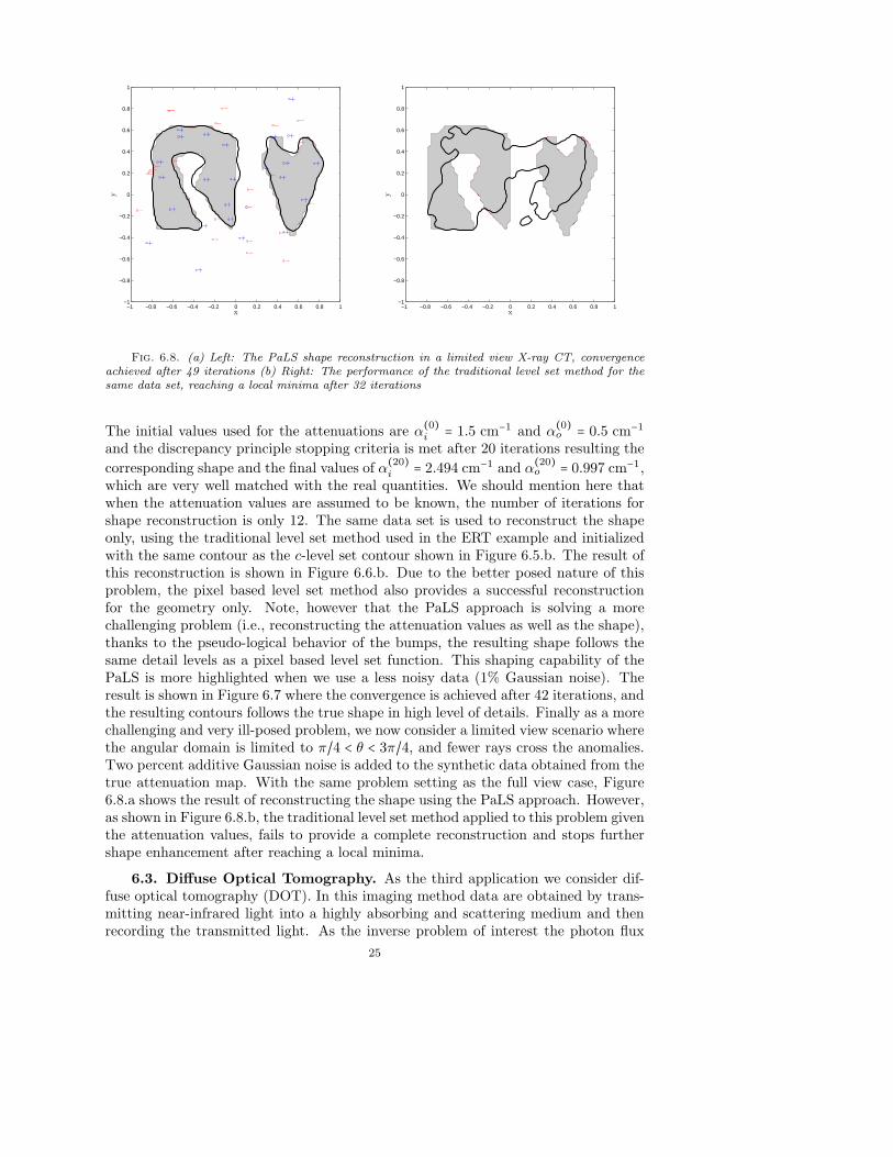
Fig. 6.8. (a) Left: The PaLS shape reconstruction in a limited view X-ray CT, convergenceachieved after 49 iterations (b) Right: The performance of the traditional level set method for thesame data set, reaching a local minima after 32 iterations

The initial values used for the attenuations are α(0)i = 1.5 cm−1 and α

(0)o = 0.5 cm−1

and the discrepancy principle stopping criteria is met after 20 iterations resulting the

corresponding shape and the final values of α(20)i = 2.494 cm−1 and α

(20)o = 0.997 cm−1,

which are very well matched with the real quantities. We should mention here thatwhen the attenuation values are assumed to be known, the number of iterations forshape reconstruction is only 12. The same data set is used to reconstruct the shapeonly, using the traditional level set method used in the ERT example and initializedwith the same contour as the c-level set contour shown in Figure 6.5.b. The result ofthis reconstruction is shown in Figure 6.6.b. Due to the better posed nature of thisproblem, the pixel based level set method also provides a successful reconstructionfor the geometry only. Note, however that the PaLS approach is solving a morechallenging problem (i.e., reconstructing the attenuation values as well as the shape),thanks to the pseudo-logical behavior of the bumps, the resulting shape follows thesame detail levels as a pixel based level set function. This shaping capability of thePaLS is more highlighted when we use a less noisy data (1% Gaussian noise). Theresult is shown in Figure 6.7 where the convergence is achieved after 42 iterations, andthe resulting contours follows the true shape in high level of details. Finally as a morechallenging and very ill-posed problem, we now consider a limited view scenario wherethe angular domain is limited to π/4 < θ < 3π/4, and fewer rays cross the anomalies.Two percent additive Gaussian noise is added to the synthetic data obtained from thetrue attenuation map. With the same problem setting as the full view case, Figure6.8.a shows the result of reconstructing the shape using the PaLS approach. However,as shown in Figure 6.8.b, the traditional level set method applied to this problem giventhe attenuation values, fails to provide a complete reconstruction and stops furthershape enhancement after reaching a local minima.

6.3. Diffuse Optical Tomography. As the third application we consider dif-fuse optical tomography (DOT). In this imaging method data are obtained by trans-mitting near-infrared light into a highly absorbing and scattering medium and thenrecording the transmitted light. As the inverse problem of interest the photon flux

25

is measured on the surface to recover the optical properties of the medium such asabsorption and/or reduced scattering functions. A well known application of thismethod is breast tissue imaging, where the differences in the absorption and scatter-ing may indicate the presence of a tumor or other anomaly [7]. For given absorptionand scattering functions a number of mathematical models have been proposed inthe literature to determine the synthetic data (photon flux) [3]. We focus on thefrequency-domain diffusion model in which the data is a non-linear function of theabsorption and scattering functions.

Consider Ω, a square with a limited number of sources on the top and a limitednumber of detectors on either the top or bottom or both. We use the diffusion modelin [3] modified for the 2D case where the photon flux u(x;ω) is related to input s(x;ω)through

−∇ ⋅ β(x)∇u(x;ω) + α(x)u(x;ω) + iωvu(x;ω) = s(x;ω), (6.9)

with the Robin boundary conditions

u(x;ω) + 2β(x)∂u(x;ω)∂ν

= 0, x ∈ ∂Ω. (6.10)

Here, β(x) denotes the diffusion, which is related to the reduced scattering functionμ′s(x), by β(x) = 1/(3μ′s(x)), α(x) denotes absorption and ∂/∂ν denotes the normal

derivative. We also have i = √−1, ω as the frequency modulation of light and v beingthe speed of light in the medium. Knowing the source and the functions α(x) andβ(x), we can compute the corresponding u(x;ω) everywhere, in particular, at thedetectors.

As the inverse problem, we consider a case that the reduced scattering functionis known and we want to reconstruct the absorption α(x) from the data. Again forthis problem we consider a point source s(x;ω) = δ(x−xs) for xs ∈ ∂Ω, which resultsin a photo flux us(x;ω) in Ω. For a measurement at xd ∈ Ω as

uds = ∫Ωus(x;ω)δ(x − xd)dx, (6.11)

the variations with respect to the variations in the absorption can be written as [3]

dudsdα

[δα] = ∫Ωδα us(x;ω) ud(x;ω)dx, (6.12)

with ud being the adjoint field caused by having the point source at xd. Identical tothe notation used for the ERT problem, consider R(α) = M(α) − u as the residualoperator where the data vector u contains the measurements of N� detectors from

M experiments. Based on (6.12) the th block of R′(α)[.] corresponding to the th

experiment is

R′�(α)[δα] = ⎛⎜⎝∫Ω δα u� u�1 dx⋮∫Ω δα u� u�N�

dx

⎞⎟⎠ , (6.13)

with u� denoting the photon flux in the th experiment and u�i being the adjointfield. For the purpose of this example we consider a very ill-posed problem whereΩ corresponds to a 5cm × 5cm imaging region, and there are only 8 point sources

26

−

+

−

+

−

+

−

+−

+

−

+−

+

−

+

−

+

−

+

x (m)

y(m

)

−0.025 −0.0125 0 0.0125 0.025

0.025

0.0125

0

−0.0125

−0.025

sources

detectors

Fig. 6.9. The 2D DOT imaging setup with the sources and detectors setting. The gray regionshows the absorption shape, while 2% Gaussian noise is added to the absorption as a heterogeneity.The dots with “+” and “-” signs correspond to the centers of positive and negative weighted bumpsin the initial state of the problem. The black contour is the resulting c-level set of the initial PaLSfunction

+

−

+

−

−

−

+

−

+

+

−

+

+

−

+

x

y

−0.025 −0.0125 0 0.0125 0.025

0.025

0.0125

0

−0.0125

−0.025

+

−

+−

−

+−

+

−

+

+

−

+

+

−

+

x

y

−0.025 −0.0125 0 0.0125 0.025

0.025

0.0125

0

−0.0125

−0.025

Fig. 6.10. (a) Left: The PaLS shape-only reconstruction, stopping criteria achieved after 152iterations in case 0.1% data noise and 2% heterogeneity (b) Right: The results of shape reconstruc-tion in case of only heterogeneity in the absorption. The evolution is manually stopped after 200iterations, showing the results

on the top and 8 detectors at the bottom. In every experiment only one of thesources is on and the measurements are performed at the bottom detectors. We haveμ′s(x) = 6 cm−1 throughout Ω. The measurements are performed at DC mode, 25 MHzand 50 MHz. The absorption binary distribution is shown in Figure 6.9 with valuesαi = 0.015 cm−1 and αo = 0.005 cm−1. To make the problem more challenging we madethe absorption distribution slightly heterogeneous by adding 2% white Gaussian noiseto it. For the PaLS setting, due to the very ill-posed nature of the problem we userelatively fewer bumps, i.e., m0 = 20. Similar to the previous two examples the centers

27

χj corresponding to positive and negative weighted bumps are taken randomly insideΩ as shown in Figure 6.9. Again to have reasonable initial support radius for thebumps the dilation factors are set to be βj = 80. Other PaLS settings are similar tothe previous examples. The forward model is solved using finite difference methodby discretizing Ω to 50 × 50 grid points. Figure 6.10.a shows the result of our shape-only reconstruction after 152 iterations, when the true absorption map is used togenerate the data and 0.1% Gaussian noise is added to it. In case of not havingany noise in the data (but still considering the heterogeneity in the absorption), theresults after 200 iterations are shown in figure 6.10.b. Although the current problemsettings make it very ill-posed and extremely hard for shape reconstruction, the PaLSapproach shows reasonable reconstructions, providing important details. For this veryill-posed problem, using the traditional level set method we failed to generate usefulreconstructions.

7. Concluding Remarks. In this paper we proposed a parametric level set ap-proach to shape based inverse problems. The basic formulation of the problem is keptgeneral, emphasizing the fact that numerically, an appropriate parametrization of thelevel set function is capable of reducing the problem dimensionality and intrinsicallyregularizes the problem. Through such modelling the level set function is more likelyto remain well behaved, and therefore there is no need to re-initialize as in traditionallevel set methods. Moreover, based on the fact that the number of underlying param-eters in a parametric approach is usually much less than the number of pixels (voxels)resulting from the discretization of the level set function, we make a use of a Newtontype method to solve the underlying optimization problem. We specifically consideredusing compactly supported radial basis functions, which used as proposed providestwo main advantages besides being parametric; first, the pseudo-logical property al-lows for recovery of wide range of shapes; and second, implicit narrow-banding forthe evolution.

Although in this paper, we only considered compactly supported radial basisfunctions as the bump functions with circular support, a combination of sufficientlysmooth bumps with various types of supports may be considered in applications wherethere is more prior information about the shape and its general geometric structure.An efficient classification of such functions for various types of shapes and problems(i.e., forming a basis dictionary) would be a future direction of research. Also for sakeof simplicity we considered only 2D problems, whereas the efficiency of a parametricapproach is more pronounced for 3D shape reconstructions where the contrast betweenthe number of voxels and the number of PaLS parameters in a parametric approachis more significant. Efficiently modelling 3D scenarios via both parametric shaperepresentation and appropriate texture and heterogeneity models is an importantfuture direction and a continuation of the current work.

Acknowledgments. This work is funded and supported by NSF, the NationalScience Foundation, under grant EAR 0838313.

REFERENCES

[1] R. Acar and CR Vogel, Analysis of bounded variation penalty methods for ill-posed problems,Inverse problems, 10 (1994), pp. 1217–1229.

[2] D. Adalsteinsson and J.A. Sethian, A fast level set method for propagating interfaces, Jour-nal of Computational Physics, (1995).

[3] SR Arridge, Optical tomography in medical imaging, Inverse problems, 15 (1999), pp. R41–R93.

28

[4] M.S. Berger, Nonlinearity and functional analysis, (1977).[5] O. Bernard, D. Friboulet, P. Thevenaz, and M. Unser, Variational B-spline level-set: a

linear filtering approach for fast deformable model evolution, IEEE Transactions on ImageProcessing, 18 (2009), pp. 1179–1191.

[6] D.P. Bertsekas, Nonlinear Programming, Athena Scientific, Belmont, MA, 1999.[7] DA Boas, DH Brooks, EL Miller, CA DiMarzio, M. Kilmer, RJ Gaudette, and

Q. Zhang, Imaging the body with diffuse optical tomography, IEEE Signal ProcessingMagazine, 18 (2001), pp. 57–75.

[8] MD Buhmann, Radial basis functions, Acta numerica, 9 (2001), pp. 1–38.[9] M. Burger, A framework for the construction of level set methods for shape optimization and

reconstruction, Interfaces and Free boundaries, 5 (2003), pp. 301–330.[10] , Levenberg-Marquardt level set methods for inverse obstacle problems, Inverse problems,

20 (2004), pp. 259–282.[11] M. Burger and S.J. Osher, A survey on level set methods for inverse problems and optimal

design, European Journal of Applied Mathematics, 16 (2005), pp. 263–301.[12] J.T. Bushberg, J.A. Seibert, E.M. Leidholdt Jr, J.M. Boone, and E.J. Goldschmidt Jr,

The essential physics of medical imaging, vol. 30, 2003.[13] J. Carrera, A. Alcolea, A. Medina, J. Hidalgo, and L.J. Slooten, Inverse problem in

hydrogeology, Hydrogeology Journal, 13 (2005), pp. 206–222.[14] T.F. CHAN, S. ESEDOGLU, and M. NIKOLOVA, Algorithms for finding global minimizers

of image segmentation and denoising models, SIAM journal on applied mathematics, 66(2006), pp. 1632–1648.

[15] T.F. Chan and X.C. Tai, Level set and total variation regularization for elliptic inverseproblems with discontinuous coefficients, Journal of Computational Physics, 193 (2004),pp. 40–66.

[16] T.F. Chan and L.A. Vese, Active contours without edges, IEEE Transactions on image pro-cessing, 10 (2001), pp. 266–277.

[17] M. Cheney, D. Isaacson, and J.C. Newell, Electrical impedance tomography, SIAM review,41 (1999), pp. 85–101.

[18] D. Colton and A. Kirsch, A simple method for solving inverse scattering problems in theresonance region, Inverse problems, 12 (1996), pp. 383–393.

[19] W. Daily and A.L. Ramirez, Electrical imaging of engineered hydraulic barriers, Geophysics,65 (2000), pp. 83–94.

[20] M.E. Davison, The ill-conditioned nature of the limited angle tomography problem, SIAMJournal on Applied Mathematics, 43 (1983), pp. 428–448.

[21] J.E. Dennis and R.B. Schnabel, Numerical methods for unconstrained optimization andnonlinear equations, Society for Industrial Mathematics, 1996.

[22] M. Di Cristo and L. Rondi, Examples of exponential instability for elliptic inverse problems,Arxiv preprint math/0303126, (2003).

[23] KA Dines and RJ Lytle, Analysis of electrical conductivity imaging, Geophysics, 46 (1981),p. 1025.

[24] O. Dorn and D. Lesselier, Level set methods for inverse scattering, Inverse Problems, 22(2006), p. R67.

[25] , Level set techniques for structural inversion in medical imaging, Deformable Models,(2007), pp. 61–90.

[26] O. Dorn, E.L. Miller, and C.M. Rappaport, A shape reconstruction method for EM tomog-raphy, Inverse problems, 16 (2000), pp. 1119–1156.

[27] H.W. Engl, M. Hanke, and A. Neubauer, Regularization of inverse problems, Kluwer Aca-demic Pub, 1996.

[28] H. Feng, W.C. Karl, and D. Castanon, A curve evolution approach to object-based tomo-graphic reconstruction, IEEE Transactions on Image Processing, 12 (2003), pp. 44–57.

[29] A. Gelas, O. Bernard, D. Friboulet, R. Prost, and V. INSA, Compactly supported radialbasis functions based collocation method for level-set evolution in image segmentation,IEEE Transactions on Image Processing, 16 (2007), pp. 1873–1887.

[30] G.H. Golub, P.C. Hansen, and D.P. O’Leary, Tikhonov regularization and total leastsquares, SIAM Journal on Matrix Analysis and Applications, 21 (2000), pp. 185–194.

[31] P.C. Hansen, Rank-deficient and discrete ill-posed problems: numerical aspects of linear in-version, Society for Industrial Mathematics, 1998.

[32] R.L. Hardy, Multiquadric equations of topography and other irregular surfaces, Journal ofGeophysical Research, 76 (1971), pp. 1905–1915.

[33] K. Ito, K. Kunisch, and Z. Li, Level-set function approach to an inverse interface problem,Inverse problems, 17 (2001), p. 1225.

29

[34] A.I. James, W.D. Graham, K. Hatfield, PSC Rao, and M.D. Annable, Optimal Estimationof Residual Non–Aqueous Phase Liquid Saturations Using Partitioning Tracer Concentra-tion Data, Water Resources Research, 33.

[35] W.A. Kalender, X-ray computed tomography, Physics in medicine and biology, 51 (2006),p. R29.

[36] E.J. Kansa, Multiquadrics–A scattered data approximation scheme with applications to compu-tational fluid-dynamics–II solutions to parabolic, hyperbolic and elliptic partial differentialequations, Computers & Mathematics with applications, 19 (1990), pp. 147–161.

[37] M.E. Kilmer, E.L. Miller, A. Barbaro, and D. Boas, 3D shape-based imaging for diffuseoptical tomography, Applied Optics, 42 (2003), pp. 3129–3144.

[38] M. Kilmer, E. Miller, M. Enriquez, and D. Boas, Cortical constraint method for diffuseoptical brain imaging, in Proceedings of SPIE, vol. 5559, 2004, p. 381.

[39] A. Kirsch, The domain derivative and two applications in inverse scattering theory, InverseProblems, 9 (1993), pp. 81–96.

[40] , Characterization of the shape of a scattering obstacle using the spectral data of the farfield operator, Inverse problems, 14 (1998), pp. 1489–1512.

[41] R. Kress and W. Rundell, A quasi-Newton method in inverse obstacle scattering, InverseProblems, 10 (1994), pp. 1145–1157.

[42] , Inverse obstacle scattering using reduced data, SIAM Journal on Applied Mathematics,59 (1998), pp. 442–454.

[43] R. Kress and A. Zinn, On the numerical solution of the three-dimensional inverse obstaclescattering problem, Journal of Computational and Applied Mathematics, 42 (1992), pp. 49–61.

[44] G. Kristensson, Inverse problems for acoustic waves using the penalised likelihood method,Inverse Problems, 2 (1986), pp. 461–479.

[45] D.J. LaBrecque, M. Miletto, W. Daily, A. Ramirez, and E. Owen, The effects of noiseon Occam’s inversion of resistivity tomography data, Geophysics, 61 (1996), pp. 538–548.

[46] A. Litman, D. Lesselier, and F. Santosa, Reconstruction of a two-dimensional binary ob-stacle by controlled evolution of a level-set, Inverse Problems, 14 (1998), pp. 685–706.

[47] G.R. Liu and X. Han, Computational inverse techniques in nondestructive evaluation, CRC,2003.

[48] AK Louis, Medical imaging: state of the art and future development, vol. 8, Institute of PhysicsPublishing, 1992.

[49] R. Marklein, K. Mayer, R. Hannemann, T. Krylow, K. Balasubramanian, KJ Langen-

berg, and V. Schmitz, Linear and nonlinear inversion algorithms applied in nondestruc-tive evaluation, Inverse Problems, 18 (2002), pp. 1733–1759.

[50] B.H. Miled and EL Miller, A projection-based level-set approach for anomaly reconstruction,Inverse Problems, 23 (2007), pp. 2375–2400.

[51] EL Miller, M. Kilmer, and C. Rappaport, A new shape-based method for object localiza-tion andcharacterization from scattered field data, IEEE Transactions on Geoscience andRemote Sensing, 38 (2000), pp. 1682–1696.

[52] EL MILLER and AS WILLSKY, A multiscale, statistically based inversion scheme for lin-earized inverse scattering problems, IEEE transactions on geoscience and remote sensing,34 (1996), pp. 346–357.

[53] V.A. Morozov and M. Stessin, Regularization methods for ill-posed problems, crc press BocaRaton, FL:, 1993.

[54] I.R. Mufti, FINITE-DIFFERENCE RESISTIVITY MODELING FOR ARBITRARILYSHAPED TWO-DIMENSIONAL STRUCTURES, Geophysics, 41 (1976), p. 62.

[55] A. Novruzi and M. Pierre, Structure of shape derivatives, Journal of Evolution Equations,2 (2002), pp. 365–382.

[56] S. Osher and R.P. Fedkiw, Level set methods and dynamic implicit surfaces, Springer Verlag,2003.

[57] S. Osher and J.A. Sethian, Fronts propagating with curvature-dependent speed: algorithmsbased on Hamilton-Jacobi formulations, Journal of computational physics, 79 (1988),pp. 12–49.

[58] W.K. Park and D. Lesselier, Reconstruction of thin electromagnetic inclusions by a level setmethod, Inverse Problems, 25 (2009), p. 085010.

[59] A. Pidlisecky, E. Haber, and R. Knight, RESINVM3D: a 3D resistivity inversion package,Geophysics, 72 (2007), p. H1.

[60] G. Pingen, M. Waidmann, A. Evgrafov, and K. Maute, A parametric level-set approachfor topology optimization of flow domains, Structural and Multidisciplinary Optimization,41 (2010), pp. 117–131.

30

[61] N. Polydorides and W.R.B. Lionheart, A Matlab toolkit for three-dimensional electricalimpedance tomography: a contribution to the Electrical Impedance and Diffuse Optical Re-construction Software project, Measurement Science and Technology, 13 (2002), pp. 1871–1883.

[62] I.T. Rekanos, T.V. Yioultsis, and T.D. Tsiboukis, Inverse scattering using the finite-element method and a nonlinear optimization technique, IEEE Transactions on MicrowaveTheory and Techniques, 47 (1999), pp. 336–344.

[63] F. Santosa, A level-set approach for inverse problems involving obstacles, ESAIM: Control,Optimisation and Calculus of Variations, 1 (1996), pp. 17–33.

[64] JH Saunders, JV Herwanger, CC Pain, MH Worthington, and CRE de Oliveira, Con-strained resistivity inversion using seismic data, Geophysical Journal International, 160(2005), pp. 785–796.

[65] J.A. Sethian et al., Level set methods and fast marching methods, Cambridge university pressCambridge, 1999.

[66] R. Snieder and J. Trampert, Inverse problems in geophysics, Springer, 1999.[67] M. Soleimani, Computational aspects of low frequency electrical and electromagnetic tomogra-

phy: A review study, International Journal of Numerical Analysis and Modeling, 5 (2008),pp. 407–440.

[68] M. Soleimani, WRB Lionheart, and O. Dorn, Level set reconstruction of conductivity andpermittivity from boundary electrical measurements using experimental data, Inverse prob-lems in science and engineering, 14 (2006), pp. 193–210.

[69] G.E. Stavroulakis, Inverse and crack identification problems in engineering mechanics,Kluwer Academic Pub, 2001.

[70] N.Z. Sun, Inverse problems in groundwater modeling, (1994).[71] X.C. Tai and T.F. Chan, A survey on multiple level set methods with applications for iden-

tifying piecewise constant functions, Int. J. Numer. Anal. Model, 1 (2004), pp. 25–47.[72] HY Tian, S. Reutskiy, and CS Chen, A basis function for approximation and the solutions

of partial differential equations, Numerical Methods for Partial Differential Equations, 24(2008), pp. 1018–1036.

[73] A.N. Tikhonov, V.Y. Arsenin, and F. John, Solutions of ill-posed problems, VH WinstonWashington, DC, 1977.

[74] AC Tripp, GW Hohmann, CM Swift, et al., Two-dimensional resistivity inversion, Geo-physics, 49 (1984), pp. 1708–1717.

[75] R. Villegas, F. Mustieles, M. Kindelan, O. Dorn, and M. Moscoso, Simultaneous char-acterization of geological shapes and permeability distributions in reservoirs using the levelset method, (2006).

[76] C.R. Vogel, Computational methods for inverse problems, (2002).[77] SY Wang, KM Lim, BC Khoo, and MY Wang, An extended level set method for shape and

topology optimization, Journal of Computational Physics, 221 (2007), pp. 395–421.[78] S. WANG and M. YU WANG, Radial basis functions and level set method for structural topol-

ogy optimization, International journal for numerical methods in engineering, 65 (2006),pp. 2060–2090.

[79] A. Webb and G.C. Kagadis, Introduction to biomedical imaging, vol. 30, 2003.[80] H. Wendland, Scattered data approximation, Cambridge University Press, 2005.[81] W.W.G. Yeh, Review of parameter identification procedures in groundwater hydrology: The

inverse problem, Water Resources Research, 22.[82] J. Zhang, R.L. Mackie, and T.R. Madden, 3-D resistivity forward modeling and inversion

using conjugate gradients, Geophysics, 60 (1995), p. 1313.[83] H.K. Zhao, T. Chan, B. Merriman, and S. Osher, A variational level set approach to

multiphase motion, Journal of computational physics, 127 (1996), pp. 179–195.[84] M.S. Zhdanov, Geophysical inverse theory and regularization problems, Elsevier Science Ltd,

2002.

31