Parametric Identification of a Base-Excited Single Pendulum

YANG LIANG and B. F. FEENYDepartment of Mechanical Engineering, Michigan State University, East Lansing, MI 48824, USA

Abstract. A harmonic balance based identification algorithm was applied to the simulated single pendulum withhorizontal base-excitation. The purpose of this simulation was to examine the applicability of the algorithm onparametrically excited, whirling chaotic systems. Modifications were adopted to adapt to the whirling systems. Thesystem was supposed to be unknown except only the excitation frequency. Linear interpolation functions and theFourier series functions were tested to approximate unknown nonlinear functions in the governing differential equation.After extracting unstable periodic orbits, all of the parameters were simultaneously identified. By direct comparison,Poincare section plots and reconstructed phase portrait techniques, it was shown that the identified system hadsimilar dynamical characteristics to the original simulated pendulum, which implies the effectiveness of the examinedalgorithm.

Keywords: parametric identification, harmonic balance method, chaotic systems, unstable periodic orbits, whirlingsystems, pendulums.

1. Introduction

A simulated, horizontally base-excited pendulum is investigated for chaotic system identification.

A harmonic balance parametric identification method is examined here, because of its simplicity

and capacity of handling chaotic data [26].

Pendulum systems are among the most thoroughly investigated dynamic systems in chaotic,

nonlinear system research (references [1–7], etc. ), for their simplicity in both theoretical expression

and experimental validation. Water [1] studied the unstable periodic orbits of a vertically excited

system. Jeong and Kim [2] investigated the bifurcation phenomena and routes to chaos of a hori-

zontally excited system. Furthermore, Bishop [3] and Dooren [4] studied the parametric regions of

chaos of a parametrically excited pendulum.

Parametric identification of nonlinear systems has seen a lot of progress in recent years. Direct

identification method [8] can be applied provided that all the displacement, velocity and accel-

eration signals are known or can be obtained. However, it is usually not so in applications, and

the method is vulnerable to noise contamination. Chen and Tomlinson [9] developed an efficient

AVD time series model, which accommodates the acceleration, velocity and displacement (AVD)

simultaneously by means of the fast Fourier transform. Plakhtienko [10, 11] introduced a method

of special weight functions, by which the second order differential equation could be converted to

a series of linear equations if some periodic orbits are known. Hence, the differential equation can

be transformed into matrix equations. Like many other studies (references [9–20]), these methods

c© 2005 Kluwer Academic Publishers. Printed in the Netherlands.

report113.tex; 25/07/2005; 21:33; p.1

focused on two types of identification procedures: random/impulse excitation response or forced

steady state periodic vibration. Furthermore, the random/impulse excitation methods based upon

the FFT and/or the frequency response function [19, 20] actually apply to weak nonlinearity due

to their assumptions. Nonlinear free vibration was also investigated for identification purposes.

Feldman [21, 24] introduced a method of utilizing the Hilbert transformation to free vibration

systems. But, it is unclear whether the Hilbert transform method can be applied to multi-degree-

of-freedom systems. Ghanem [25] proposed an algorithm based on wavelet analysis. The algorithm

was tested on single and multi-degree of freedom (d. o. f. ) systems, and was proven effective for

free and forced non-chaotic vibration. The wavelet analysis method is based upon the orthogonality

of the wavelet basis functions, it is thus essentially similar to the harmonic balance method, which

utilizes the orthogonality of the Fourier series orthonormal functions. The wavelet basis functions

are time localized, while the harmonic basis functions apply to the entire duration of time. Recently,

a method [22, 23] which exploits proper orthogonal decomposition (POD) and optimization was

developed for nonlinear systems and tested on simple chaotic systems. Meanwhile, based upon the

harmonic balance method [15–18], Feeny and Yuan [26, 27] proposed a method for chaotic systems,

which also exploits the extracted unstable periodic orbits. This method was successfully applied to

single degree of freedom systems, and is theoretically applicable to chaotic or non-chaotic, strongly

nonlinear multi-degree of freedom systems. Thus, this study is to present new research results by

applying the method to more complicated chaotic systems. As we know, the harmonic balance

method requires periodic responses for identification purposes. For linear systems, the method can

be simplified to frequency response functions (FRF) method if periodic responses can be obtained

at multiple frequencies. For non-chaotic, nonlinear systems, the harmonic balance method also

have advantages over other methods due to its simple algorithm and/or the resistance to noise

contamination. For chaotic systems, the chaotic response is no-periodic. However, for hyperbolic

chaos, if unstable periodic orbits (UPOs) lie within, we can extract the approximated unstable

periodic orbits from the chaotic data. Hence, the harmonic balance identification can be applied

based upon the UPOs. On the other hand, many other identification methods can not be applied to

chaotic systems. Noticeably, the wavelet analysis method [25] can also be applied for chaotic system

since both the wavelet method and the harmonic balance method are based upon orthonormal basis

and signal reconstruction. The harmonic balance method has simpler algorithm and is easier for

industry applications. The wavelet analysis, on the other hand, is more suitable for identification

of the time-variant parameters. Since our present study focused on systems with time-invariant

parameters, the harmonic balance method is a more suitable choice.

2

Our purpose here is to apply the harmonic balance algorithm to the horizontally excited

pendulum system such that we can examine the algorithm applicability on systems with chaotic

whirling behavior and strong nonlinearity. Also, the single pendulum was investigated due to its

simplicity in simulation and experiment verification. The identification method has been examined

on smooth excitation single d. o. f. systems with simple nonlinearity [26]. However, the pendulum is

a more complicated case, and the algorithm must be modified. In the following sections, the single

pendulum system and the modified method will be introduced first. Pre-requirements of applying

this method will be discussed, primarily regarding the phase plane reconstruction. In the last two

sections, the simulation results will be presented and discussed.

2. Horizontally excited single pendulum & identification algorithm

Single pendulum systems have simple structures, but strong non-linearity due to their whirling

property. The governing differential equations can be simulated easily, and the experimental veri-

fication is also feasible. Based upon these advantages, horizontally base excited single pendulums

are chosen for investigation here. The non-dimensional form of the differential equation is

θ + 2ξ/rθ + 1/r2 sin θ − f sin t cos θ = 0, (1)

where t = ωτ , ω is the angular excitation velocity, and τ is the actual time; ξ is the viscous

damping coefficient; r = ω/ωN , ωN =√

mgeJ is the natural frequency of the linearized system, m

is the pendulum mass, e is the the centroid offset from the pendulum hinge, J is the moment of

inertia about the hinge point. Meanwhile coefficient f = meJ a, and a is the excitation amplitude.

For simplicity, we denote cr = 2ξ/r as the new non-dimensional friction coefficient. The function

f sin t cos θ is the nonlinear parametric excitation term, and 1/r2 sin θ is the autonomous nonlinear

part. The angular displacement θ is in S[ − π, π)1 space (one dimensional sphere space), whereas

the angular velocity and acceleration are in R1 space.

To apply the identification algorithm [26] to the pendulum system, the following more general

expression of (1) can be assumed:

crx + kx + fanl(x, x) + {d1 + fpnl(x, x)}p(t) = −x, (2)

where k is the linear stiffness parameter, fanl(x, x) is the autonomous nonlinear part, fpnl(x, x) is

the time-independent part of the parametric excitation term, and coefficient d1 is the amplitude of

external excitation force. If d1 is non-zero and fpnl equal to zero, the system becomes a nonlinear

system with external excitation force. On the contrary, if d1 is zero and fpnl is non-trivial, it is

3

then a parametrically excited system. For the examined single pendulum, parameter k = 0 and

d1 = 0. Meanwhile, since the non-linearity of the pendulum is caused by geometry, it is convenient

to assume fanl and fpnl in equation (2) as functions of only displacement, such that

crx + fanl(x) + fpnl(x)p(t) = −x. (3)

Based on equation (3), it is assumed that nothing is known a priori except the harmonic

excitation term p(t) = α1 cosωt + β1 sinωt. Unknown functions fpnl and fanl can be approximated

by

fpnl ≈N∑

i=1

Piφi(x), (4)

fanl ≈N∑

i=1

qiφi(x), (5)

where {φi(x)} is a set of basis functions, and Pi, qi are unknown parameters. Since the choice of

basis functions can affect accuracy of the identified functions, two sets of basis functions were tested

in the simulation: linear interpolation functions and Fourier series functions.

Substituting (4), (5) and harmonic excitation into (3), we have

crx +N∑

i=1

qiφi(x) +N∑

i=1

niφi(x) cos t +N∑

i=1

piφi(x) sin t = −x, (6)

where ni = Piα1 and pi = Piβ1. With equation (6), harmonic balance identification [26] can be

applied after extracting unstable or stable periodic orbits from the collected displacement data. For

a period k orbit, if x in R1 (one dimensional real space), the displacement, velocity and acceleration

signals can be approximated by the following truncated Fourier series expansions:

xk(t) ≈ a0,k

2+

M∑

j=1

(aj,k cosjωt

k+ bj,k sin

jωt

k), (7)

xk(t) ≈M∑

j=1

jω

k(−aj,k sin

jωt

k+ bj,k cos

jωt

k), (8)

xk(t) ≈M∑

j=1

−j2ω2

k2(aj,k cos

jωt

k+ bj,k sin

jωt

k), (9)

where, for non-dimensional equation (6), ω = 1. However, for x in S1 (one dimensional sphere space,

such as angular displacement θ in the single pendulum), Equations (7) – (9) are not applicable.

The harmonic balance method can still be applied here, but a modification is needed to derive the

velocity and acceleration R1 signals from the sampled S1 displacement signal.

4

0 0.5 1 1.5 23

2

1

0

1

2

3

period(a)

angl

e

0 0.5 1 1.5 210

8

6

4

2

0

2

4

period(b)

angl

e

0 0.5 1 1.5 215

10

5

0

5

10

period(c)

angl

e

Figure 1. A period-4 orbit (a) sampled signal; (b) actual continuous signal xc; (c) · · · constant rotation part ωckt, –oscillatory part xvar.

Consider an experiment in which whirling angle θ is sensed with an encoder such that the

output x has values in the interval [−π, π). Thus, x = θmod(2π)−π is discontinuous. According to

the illustration in Figure 1 of a period four orbit of the single pendulum system, the sampled data

{x} should be converted to a continuous signal {xc} in R1, and then decomposed as

xck = ωckt + xvar,k,

where ωckt represents the constant rotating part of a whirling periodic orbit, and xvar,k is the

oscillatory part of the orbit signal, which can be approximated by the truncated Fourier series

expansion

xvar,k(t) ≈ u0,k

2+

M∑

j=1

(uj,k cosjωt

k+ vj,k sin

jωt

k).

5

Based upon xck, the corresponding velocity and acceleration can be expressed as

xk(t) ≈ ωck +M∑

j=1

jω

k(−uj,k sin

jωt

k+ vj,k cos

jωt

k), (10)

xk(t) ≈M∑

j=1

−j2ω2

k2(uj,k cos

jωt

k+ vj,k sin

jωt

k). (11)

Meanwhile, for a period-k orbit, if φi(x): S1 → C[−1, 1], as in the case of the pendulum, then

continuous functions φi(xk), φi(xk) cos t and φi(xk) sin t can also be approximated by

φi(xk) ≈ ci0,k

2+

M∑

j=1

(cij,k cosjωt

k+ dij,k sin

jωt

k), (12)

φi(xk) cos t ≈ ei0,k

2+

M∑

j=1

(eij,k cosjωt

k+ fij,k sin

jωt

k), (13)

φi(xk) sin t ≈ gi0,k

2+

M∑

j=1

(gij,k cosjωt

k+ hij,k sin

jωt

k). (14)

Substituting (10)–(14) into (6), the differential equation can be transformed into the following

matrix equation for a period-k orbit

ωck e10,k/2 g10,k/2 c10,k/2 · · · eN0,k/2 gN0,k/2 cN0,k/2ωk v1,k e11,k g11,k c11,k · · · eN1,k gN1,k cN1,k

−ωk u1,k f11,k h11,k d11,k · · · fN1,k hN1,k dN1,k...

......

.... . .

......

...Mωk vM,k e1M,k g1M,k c1M,k · · · eNM,k gNM,k cNM,k

−Mωk uM,k f1M,k h1M,k d1M,k · · · fNM,k hNM,k dNM,k

·

cr

n1

p1

q1...

nN

pN

qN

=

0ω2

k2 u1,kω2

k2 v1,k...

M2ω2

k2 uM,kM2ω2

k2 vM,k

.

(15)

For simplicity, Ak is denoted as the left-hand side matrix,

λ = ( cr n1 p1 q1 · · · nN pN qN )T ,

and

βk = ( 0 ω2

k2 u1,kω2

k2 v1,k · · · M2ω2

k2 uM,kM2ω2

k2 vM,k )T .

6

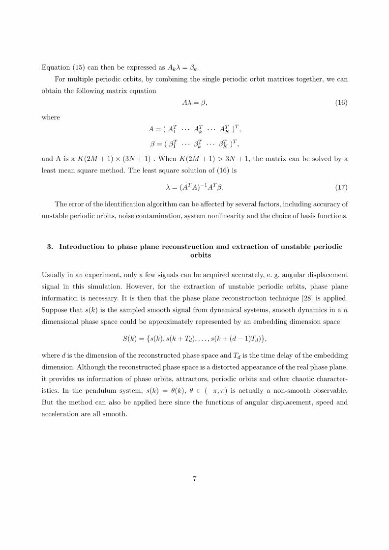
Equation (15) can then be expressed as Akλ = βk.

For multiple periodic orbits, by combining the single periodic orbit matrices together, we can

obtain the following matrix equation

Aλ = β, (16)

where

A = ( AT1 · · · AT

k · · · ATK )T ,

β = ( βT1 · · · βT

k · · · βTK )T ,

and A is a K(2M + 1) × (3N + 1) . When K(2M + 1) > 3N + 1, the matrix can be solved by a

least mean square method. The least square solution of (16) is

λ = (AT A)−1AT β. (17)

The error of the identification algorithm can be affected by several factors, including accuracy of

unstable periodic orbits, noise contamination, system nonlinearity and the choice of basis functions.

3. Introduction to phase plane reconstruction and extraction of unstable periodicorbits

Usually in an experiment, only a few signals can be acquired accurately, e. g. angular displacement

signal in this simulation. However, for the extraction of unstable periodic orbits, phase plane

information is necessary. It is then that the phase plane reconstruction technique [28] is applied.

Suppose that s(k) is the sampled smooth signal from dynamical systems, smooth dynamics in a n

dimensional phase space could be approximately represented by an embedding dimension space

S(k) = {s(k), s(k + Td), . . . , s(k + (d− 1)Td)},

where d is the dimension of the reconstructed phase space and Td is the time delay of the embedding

dimension. Although the reconstructed phase space is a distorted appearance of the real phase plane,

it provides us information of phase orbits, attractors, periodic orbits and other chaotic character-

istics. In the pendulum system, s(k) = θ(k), θ ∈ (−π, π) is actually a non-smooth observable.

But the method can also be applied here since the functions of angular displacement, speed and

acceleration are all smooth.

7

3.1. Choosing the embedding dimension and time delay

The time delay value Td can be obtained from average mutual information function [28], which is

expressed as

IAB(t) =∑

ai,bk

PAB(ai, bk)log2

PAB(ai, bk)PA(ai)PB(bk)

, (18)

where t is the time lag, ai is the sampled data s(i), A is the set of {s(i)}, k = i + T , bk is thus

s(i + t), and B is considered as the set of {s(i + t)}. Meanwhile, PA(x) is the probability function

of observing x out of a set A, PB(y) is the probability of observing y out of a set B, and PAB(x, y)

is the joint probability function of observing x and y out of A and B. After calculating I(t), the

best time delay Td is chosen when I(t) reaches its first minimum. To determine the value of dE for

minimum required delay dimensions, the false nearest neighborhood method was applied [28].

3.2. Extracting Unstable Periodic Orbits (UPOs)

There are numerous unstable periodic orbits in a chaotic signal. The reconstructed phase space can

be used to extract the hidden UPOs. Since the horizontally excited single pendulum is excited by

a harmonic signal with period T , the UPOs will have the periodicity of integer multiples of the

excitation period T . Though theoretically, no exact UPO can be found through the collected data,

the theory proved that some very close approximation of the UPO exists provided that the data is

long enough. With the error tolerance e set for UPO extraction, we say that a approximated UPO

of period k is extracted if |S(n− kT )−S(n)|c < e. Noticing that in S1 space, the distance between

two points, x and y, is measured on a circle, and thus can be expressed as

|x− y|c = |(π + |x− y|mod2π)− π|. (19)

Usually e is set as 1–5% of the span of the data [26], and the smaller e value is always desirable if

possible, since the corresponding UPOs will be closer to the real periodic orbits.

4. Numerical simulation of the horizontally excited pendulum

4.1. Phase plane reconstruction

The simulation was based upon the non-dimensional differential equation (1). A data set of 30000

points was gathered with a sampling rate fs = 25/T . Displayed in Figure 2 (a) is the 2-D recon-

structed phase space. The coefficients were chosen as f = 1.52, c = 0.03, r = 0.8333. The actual

minimum embedding dimension needed for a complete phase plane reconstruction was found to be

8

−4 −2 0 2 4−4

−2

0

2

4

theta(t)

thet

a(t+

5)

−4 −2 0 2 4−4

−2

0

2

4

theta(t)

thet

a(t+

dt)

(a) (b)

Figure 2. Reconstructed phase plane (a) and Poincare section plot (b); θ(t) is represented by theta(t) in the plots.

0 5 10 15 20 250

0.5

1

1.5

2

2.5

dt

I(dt

)

Mutual Information

Figure 3. Mutual information of the data; the first minimum is at dt=5.

four. However, since our purpose of reconstructing phase plane is to extract UPOs, which compare

points with kT time interval (implying the addition of the S1 dimension of time), the possibility of

false nearest neighbor is then greatly reduced. Hence, two embedding coordinates are adequate for

this case, and also simpler for display purposes.

Meanwhile, according to Figure 3 of average mutual information, the calculated best time delay

was Td = 5. The Poincare section is displayed in Figure 2 (b). The Poincare section plot provides us

9

3 2 1 0 1 23

2

1

0

1

2

theta(t)(a)

thet

a(t+

dt)

4 2 0 2 43

2

1

0

1

2

3

4

theta(t)(b)

thet

a(t+

dt)

4 2 0 2 44

2

0

2

4

theta(t)(c)

thet

a(t+

dt)

4 2 0 2 44

2

0

2

4

theta(t)(d)

thet

a(t+

dt)

Figure 4. (a)A period-1 orbit; (b) A period-2 orbit; (c) A period-2 orbit; (d) A period-2 orbit.

a handy tool to visually compare chaotic properties of different systems. Similar Poincare section

plots give evidence of similar dynamical behaviors of the systems.

4.2. Parametric identification

For simplicity, the data used in identification process was noise-free, thus excluding the noise-

generated error in the identified parameters. The UPOs were extracted before applying identification

algorithm. An error tolerance of e = 3% was applied in the extraction. The error tolerance can be

made smaller if longer sampled data is available. Consequently, around 25 UPOs were extracted

from period 1 to period 16. Figure 4 shows a example of periodic orbits of period one and two.

Some are whirling orbits, whereas others are oscillating orbits. With the UPOs extracted, in the

identification process, two sets of basis functions were tested to approximate the unknown nonlinear

functions in the governing equation.

10

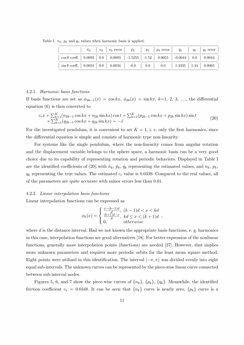
Table I. nk, pk and qk values when harmonic basis is applied.

– nk nk nk error pk pk pk error qk qk qk error

cos θ coeff. 0.0093 0.0 0.0093 -1.5255 -1.52 0.0055 -0.0044 0.0 0.0044

sin θ coeff. 0.0034 0.0 0.0034 -0.0 0.0 0.0 1.4335 1.44 0.0065

4.2.1. Harmonic basis functions

If basis functions are set as φ2k−1(x) = cos kx, φ2k(x) = sin kx, k=1, 2, 3, . . ., the differential

equation (6) is then converted to

crx +∑K

k=1(n2k−1 cos kx + n2k sin kx) cos t +∑K

k=1(p2k−1 cos kx + p2k sin kx) sin t

+∑K

k=1(q2k−1 cos kx + q2k sin kx) = −x. (20)

For the investigated pendulum, it is convenient to set K = 1, i. e. only the first harmonics, since

the differential equation is simple and consists of harmonic type non-linearity.

For systems like the single pendulum, where the non-linearity comes from angular rotation

and the displacement variable belongs to the sphere space, a harmonic basis can be a very good

choice due to its capability of representing rotation and periodic behaviors. Displayed in Table I

are the identified coefficients of (20) with nk, pk, qk representing the estimated values, and nk, pk,

qk representing the true values. The estimated cr value is 0.0339. Compared to the real values, all

of the parameters are quite accurate with minor errors less than 0.01.

4.2.2. Linear interpolation basis functions

Linear interpolation functions can be expressed as

φk(x) =

x−(k−1)dd , (k − 1)d < x < kd

(k+1)d−xd , kd ≤ x < (k + 1)d

0, otherwise

,

where d is the distance interval. Had we not known the appropriate basis functions, e. g. harmonics

in this case, interpolation functions are good alternatives [18]. For better expression of the nonlinear

functions, generally more interpolation points (functions) are needed [27]. However, that implies

more unknown parameters and requires more periodic orbits for the least mean square method.

Eight points were utilized in this identification. The interval [−π, π) was divided evenly into eight

equal sub-intervals. The unknown curves can be represented by the piece-wise linear curve connected

between sub-interval nodes.

Figures 5, 6, and 7 show the piece-wise curves of {nk}, {pk}, {qk}. Meanwhile, the identified

friction coefficient cr = 0.0348. It can be seen that {nk} curve is nearly zero, {pk} curve is a

11

−4 −3 −2 −1 0 1 2 3 4−1

−0.8

−0.6

−0.4

−0.2

0

0.2

0.4

0.6

0.8

1

theta position

nk

Figure 5. nk curve for linear interpolation basis; (*) identified values, (—) true function.

−4 −3 −2 −1 0 1 2 3 4−2

−1.5

−1

−0.5

0

0.5

1

1.5

2

theta position

Pk

Figure 6. pk curve for linear interpolation basis; (*) identified values, (—) true function.

12

−4 −3 −2 −1 0 1 2 3 4−2

−1.5

−1

−0.5

0

0.5

1

1.5

theta position

Qk

Figure 7. qk curve for linear interpolation basis; (o) identified values, (—) true function.

cosine curve, and the {qk} curve is a sine curve, which are consistent with the differential equation

(1). However, eight points are still a rough representation of the real curve, and consequently the

interpolation functions introduces more error than the harmonic basis case. In the next section, we

will discuss the error’s influence on the dynamic characteristics of the system.

5. Discussion and Validation

Direct comparison showed that the identification algorithm was satisfying for the single degree of

freedom system. Furthermore, it was the harmonic basis that generated the more precise identifi-

cation result, due to the fact that the unknown nonlinear functions consist of harmonics. However,

when investigating unknown systems, direct comparison is unavailable. In this case, it is then

natural to examine the dynamical behavior, e. g. chaotic characteristics, of the identified system

for validation purposes.

Displayed in Figure 8 (a) and (b) are Poincare sections of the identified systems with harmonic

basis and linear interpolation basis. The Poincare sections look similar to the original pendulum,

which implies the dynamical similarity of these three chaotic systems. Thus, for the description of

chaotic characteristics, the linear interpolation approximation, though a coarse representation, is

still acceptable.

13

−4 −2 0 2 4−4

−2

0

2

4

theta(t)

thet

a(t+

dt)

−4 −2 0 2 4−4

−2

0

2

4

theta(t)

thet

a(t+

dt)

(a) (b)

Figure 8. Poincare section plots of identified systems: (a) by linear interpolation basis, (b) by Harmonic basis.

For more validation methods of the unknown systems, we can also refer to the linearized model,

comparison of fractal dimensions, vector fields [27], bifurcation diagrams, and Lyapunov exponents.

But for this simulation case, where the parameters are known, direct comparison of parameters is

the best tool.

6. Conclusions

In this paper, the simulated parametric identification procedure was investigated on a chaotic

system of a horizontally base excited pendulum. Theoretically, the identification algorithm can

be applied to single degree of freedom system with a known excitation frequency and unknown

parametric, or forced excitation functions. The identification algorithm [26, 27] was modified and

improved for application to the whirling pendulum system with parametric excitation. Two types

of basis functions were applied to approximate the unknown functions. Then, the simulations of

the identified models were presented to verify the effectiveness of the algorithm.

The direct comparison of both parameters and Poincare sections showed the accuracy of the

identified parameters and the similarity between the original and the identified systems. Although

both of the methods gave similar results, the harmonic basis functions matched the form of the

true nonlinearity, and therefore in this case, gave a more precise result. On the other hand, the

linear interpolation was also shown to be valuable since it is a good choice for a general unknown

type of non-linearity in a single variable.

According to the simulation result, the improved parametric identification process was success-

ful in single degree-of-freedom parametrically excited whirling systems. It is also promising to apply

14

this method to more general dynamic systems, such as rotational and/or multi-degree-of-freedom

systems. For this study, the simulation was limited to single degree of freedom systems with no

noise contamination. Hence, the error and convergence analysis was not addressed in this study.

However, we do know that to obtain more accurate identification results, more accurate UPOs

are necessary, i. e. small recurrence error in the UPO extraction. For more general applications,

multi-degree of freedom systems and experimental verifications are needed for full investigation of

the proposed method.

Acknowledgements

We would like to express our appreciation to NASA (grant number NAG-1-01048, with Dr. Walt

Silva) for supporting this research.

References

1. Willem van de Water, Marc Hoppenbrouwers, ‘Unstable periodic orbits in the parametrically excited pendulum’,Physical Review A, Vol. 44(10), 1991, pp. 6388–6397.

2. Jaeyong Jeong, Sang-Yoon Kim, ‘Bifurcations in a Horizontally Driven Pendulum’, Journal of Korean PhysicalSociety, Vol. 35(5), 1999, pp. 393–398.

3. S. R. Bishop, M. J. Clifford, ‘Zones of Chaotic Behavior in the parameterically excited pendulum’, Journal ofSound and Vibration, Vol. 189, 1996, pp. 142–147.

4. R. V. Dooren, ‘Chaos in a pendulum with forced horizontal support motion: a tutorial’, Chaos, Solutions &Fractals, Vol. 7(1), 1996, pp. 77–90.

5. V. B. Raybov, ‘Using Lyapunov exponents to predict the onset of chaos in nonlinear oscillators’, Physical ReviewE, Vol. 66(1), No. 016214, Part 2, 2002.

6. W. Szemplinska-Stupnicka, E. Tyrkiel, ‘The oscillation-rotation attractors in the forced pendulum and theirpeculiar properties’, International Journal of Bifurcation and Chaos, Vol. 12(1), 2002, pp. 159–168.

7. M. Clerc, P. Coullet, E. Tirapegui, ‘The stationary instability in quasi-reversible systems and the Lorenzpendulum’, International Journal of Bifurcation and Chaos, Vol. 11(3), 2001, pp. 591–603.

8. K. S. Mohammad and et al., ‘Direct parameter estimation for linear and non-linear structures,’ Journal of Soundand Vibration, vol. 153(3), 1992, pp. 471–499.

9. Q. Chen, G. R. Tomlinson, ‘Parametric identification of systems with dry friction and nonlinear stiffness a timeseries model’, Journal of Vibration and Acoustics, Vol. 118 (2), 1996, pp. 252–263.

10. N. P. Plakhtienko, ‘Methods of identification of nonlinear mechanical vibrating systems’, International AppliedMechanics, Vol. 36 (12), 2000, pp. 1565–1594

11. N. P. Plakhtienko, ‘A method of special weight-functions in the problem of parametric identification ofmechanical systems’, DOPOV AKAD NAUK A, Vol. 8, 1983, pp. 31–35.

12. R. K. Kapania, and S. Park, ‘Parametric identification of nonlinear structural dynamic systems using time finiteelement method’, AIAA Journal, Vol. 35 (4), 1997, pp. 719–726

13. G. Verbeek, A. Dekraker, D. H. Vancampen, ‘Nonlinear parametric identification using periodic equilibriumstates - application to an aircraft landing gear damper’, Nonlinear Dynamics, Vol. 7 (4), 1995, pp. 499–515.

14. M. R. Hajj, J. Fung, A. H. Nayfeh, et al. , ‘Parametric Identification of Nonlinear Dynamic Systems’, Computers& Structures, Vol. 20 (3), 1985, pp. 487–493.

15. K. Yasuda, S. Kawamura, and K. Watanabe, ‘Identification of nonlinear multi-degree-of-freedom systems(presentation of a technique)’, JSME International Journal, Series III, Vol 31, 1988, pp. 8–14.

15

16. K. Yasuda, S. Kawamura, 1989, ‘A nonparametric identification technique for nonlinear vibratory systems(proposition of a technique)’, JSME International Journal, Series III, Vol 31, 1989, pp. 365–372.

17. K. Yasuda, K. Kamiya, ‘Identification of a nonlinear beam (proposition of an identification technique)’, JSMEInternational Journal, Series III, Vol 33, 1990, pp. 535–540.

18. K. Yasuda, K. Kamiya, ‘Experimental identification technique of nonlinear beams in time domain’, NonlinearDynamics, Vol. 18, 1997, pp. 185–202.

19. G. Kerschen, V. Lenaerts, J. C. Golinval, ‘Identification of a continuous structure with a geometrical non-linearity. Part I: Conditioned reverse path method’, Journal of Sound and Vibration, Vol. 262(4), 2003, pp. 889–906.

20. C. M. Richard, R. Singh, ‘Identification of multi-degree-of-freedom non-linear systems under random excitationsby the reverse-path spectral method’, Journal of Sound and Vibration, Vol. 213(4), 1998, pp. 673–708.

21. Michael Feldman, ‘Non-linear system vibration analysis using Hilbert transform–I. free vibration analysis method“FREEVIB” ’, Mechanical Systems and Signal Processing, Vol. 8(2), 1994, pp. 119–127.

22. V. Lenaerts, G. Kerschen, J. -C. Golinval, ‘Identification of a continuous structure with a geometrical non-linearity. Part II: Proper orthogonal decomposition’, Journal of Sound and Vibration, Vol. 262(4), 2003, pp. 907–919.

23. G. Kerschen, B. F. Feeny, J. C. Golinval, 2003, ‘On the exploitation of chaos to build reduced-order models’,Computer Methods in Applied Mechanics and Engineering, Vol. 192(13-14), 2003, pp. 1785–1795.

24. M. Feldman, 1997, ‘Non-linear free vibration identification via the Hilbert transform’, Journal of Sound andVibration, Vol. 208(3), 1997, pp. 475–489.

25. Roger Ghanem, F. Romeo, 2001, ‘A wavelet-based approach for model and parameter identification of nonlinearsystems’, International Journal of Non-linear Mechanics, Vol. 36, 2001, pp. 835–859.

26. C. M. Yuan, B. F. Feeny, ‘Parametric Identification of Chaotic Systems’, Journal of Vibration and Control, Vol.4(4), 1998, pp. 405–426.

27. B. F. Feeny, C. M. Yuan, J. P. Cusumano, ‘Parametric identification of an experimental magneto-elasticoscillator’, Journal of Sound and Vibration, Vol. 247(5), 2001, pp. 785–806.

28. H. D. I. Abarbanel, R. Brown, J. J. SIDorowich, L. S. Tsimring, ‘The analysis of observed chaotic data inphysical systems’, Reviews of Modern Physics, Vol. 65, 1993, pp. 1331–1392.

16