ORIGINAL PAPER - PRODUCTION ENGINEERING

Parametric analysis of diffusivity equation in oil reservoirs

Reza Azin1 • Mohamad Mohamadi-Baghmolaei1 • Zahra Sakhaei1

Received: 5 November 2015 / Accepted: 2 April 2016 / Published online: 15 April 2016

� The Author(s) 2016. This article is published with open access at Springerlink.com

Abstract The governing equation of fluid flow in an oil

reservoir is generally non-linear PDE which is simplified as

linear for engineering proposes. In this work, a compre-

hensive numerical model is employed to study the role of

non-linear term in reservoir engineering problems. The

pervasive sensitivity analysis is performed on rock and

fluid properties, and it is shown that rock permeability and

fluid viscosity are the most significant parameters which

influence the pressure profile. Moreover, the critical

reservoir radius was determined in four different cases

including heavy and light oil along with high and low

permeable rocks, in which the pressure difference of linear

and non-linear diffusivity equation is significant. Results of

this study give an insight into proper simplification of

diffusivity equation and provide an engineering-based

decision strategy for different reservoir properties having

certain rock and fluid properties in oil reservoirs. The

results show the significance of depletion time, production

rate, and reservoir radius in calculation of pressure drop.

Keywords Diffusivity equation � Non-linear partialdifferential equation � Numerical solution � Analyticalsolution

List of symbols

B Formation volume factor, bbl/STB

C Compressibility factor, psi-1

h Formation thickness, ft

K Absolute permeability, mD

p Pressure, psi

Q Flow rate, STB/day

q Constant rate, STB/day

r Radius, ft

t Time, h

Greek symbols

l Viscosity, cp

g Diffusivity constant

q Gas density, lb/ft3

[ Porosity

m Apparent fluid velocity, bbl/day-ft2

Subscripts

c Critical

e External

f Formation

i Initial

o Oil

pss Pseudo steady-state

sc Standard condition

t Total

w Wellbore

Abbreviations

L Linear

NL Non-linear

Introduction

Understanding the trend of pressure profile in a reservoir

during primary depletion is essential in reservoir studies.

Especially, for those reservoirs which are susceptible to

perform two phases of hydrocarbon due to pressure drop

& Reza Azin

reza.azin@pgu.ac.ir

1 Department of Chemical Engineering, Faculty of Petroleum,

Gas and Petrochemical Engineering, Persian Gulf University,

Bushehr, Iran

123

J Petrol Explor Prod Technol (2017) 7:169–179

DOI 10.1007/s13202-016-0247-5

(Danesh 1998). In this regard, any precise approach and

model which include less assumption can be a reliable

method. The fluid flow in reservoir or in porous medium

has been a great interest of physicists, engineers and

hydrologists who tried to predict the behaviors of com-

pressible and incompressible fluids. They have designed

several experiments so as to validate the implementation of

their proposed correlations (Ahmed 2011). The basic

equation for predicting pressure distribution in a reservoir

is the diffusivity equation. For this equation, the reservoir

temperature is supposed to be constant which is a valid

assumption in most cases. Several methods have presented

to solve the diffusivity equation including numerical and

analytical approaches. The diffusivity equation is also

solved in dimensionless form (Lee 1996).

Several procedures have been proposed to solve the

pressure diffusivity equation. Take Chakrabarty et al.

(1993) as an example, who provided a quantitative analysis

of the effects of neglecting the quadratic gradient term on

solving the diffusion equation governing the transient state

(Chakrabarty et al. 1993). It should be noted that among the

flow regimes in reservoir, the transient flow is the most

significant state upon which such important characteristics

as permeability, reservoir capacity, and skin factor can be

determined using well test analysis (Van Everdingen 1953;

Lee 1992). Regarding this specification, Liang et al.

applied the transient pulse decay to measure the perme-

ability of tight rocks and synthetic materials using the

pressure diffusion equation, in which due to dependent

pressure of gas compressibility the diffusivity equation

became non-linear (Liang et al. 1978). They also consid-

ered the Klinkenberg effect in their computations. Another

common application of diffusivity equation is during

pressure transient analyses. Goode offered an analytic

solution for three dimensional diffusivity equations during

drawdown and buildup of a horizontal model to get some

specifications of reservoir. He applied numerical solution

for validation of his procedure (Goode 1987). In some

cases, the researchers face with heterogeneous reservoirs

instead of homogeneous, therefore, they use some synthetic

methods to solve the problem (Dake 1983). Loucks et al.

solved diffusivity equation using Laplace transformation

for finding pressure drop characteristics in a composite

system with different permeabilities (Loucks and Guerrero

1961). Also, van Everdingen and Hurst proposed that by

use of Laplace transform instead of tedious prior mathe-

matical analysis, the problems encounter with flow equa-

tions can be simplified (Van Everdingen and Hurst 1949).

It should be noted that, as the non-linear form of dif-

fusivity equation causes difficulties in solution process

(Odeh and Babu 1988). To overcome these difficulties

several suggestions and methods have been proposed such

as that of Vik and Jelmert, who planned a solution using

pressure logarithm transform for diffusivity equation

included pressure squared term (Jelmert and Vik 1996).

Xu-Long et al. in their study found the exact solution for

radial fluid flow along with pressure squared term. They

considered both types of inner boundary conditions, con-

stant flow rate and constant pressure. The generalized

Weber transform has been used in their study. They also

proposed the analytical solution using Hankel transform for

fluid flow in spherical state when the pressure squared term

is included. Their researches consisted of analyzing and

comparing the linear and non-linear diffusivity equation.

Their results showed that, the differences between pres-

sures which had been obtained by two types of equations

reaches about 8 present for long time (Xu-long et al. 2004).

Another interesting illustration in this category is the work

done by Braeuning et al. who applied modified logarithm

transform for solving diffusivity equation. They considered

the damage skin and wellbore storage in their solution.

They noticed that, the magnitude of error as result of lin-

earization of diffusivity equation depends on the wellbore

damage, the pseudo-skin due to partial penetration and

non-linear flow parameter (Braeuning et al. 1998). Other

example is the usage of Laplace transform in analytical

solution of non-linear diffusivity equation which was done

by Dusseault and Wang. They claimed that the observed

deviation of their approach from existing solutions was

occurred due to high pressure gradient, compressibility of

the core and the injected fluids (Wang and Dusseault 1991).

These kinds of approximations and considerations may

cause some changes in pressure drop profile along the

radius of reservoir which may be significant or not. On this

subject in the current study first, the comparison between

analytical and numerical solution for both linear and non-

linear diffusivity equation will be performed at wellbore

radius, and second the comprehensive sensitivity analysis

will be done to find the significant physical properties of

reservoir which influence the pressure drop. Next, a com-

prehensive analysis of involved parameters such as deple-

tion time, reservoir radius and production rate will be

performed to find where the pressure differences of linear

and non-linear diffusivity equations are significant.

Mathematical considerations

For slightly compressible, unsteady-state fluid flow through

a radial reservoir, the diffusivity equation is written as

(Ahmed 2011). For more details, refer to ‘‘Appendix 1’’:

o2p

or2þ 1

r

op

orþ c

op

or

� �2

¼ 1

gop

otð1Þ

170 J Petrol Explor Prod Technol (2017) 7:169–179

123

Many authors neglect the opor

� �2

term assuming small

magnitude of compressibility factor and make Eq. 1 linear.

This assumption may be valid for slightly compressible

fluids. However, when either compressibility factor or

pressure gradient terms are large, the non-linear term

cannot be removed from diffusivity equation and makes the

PDE non-linear. In this paper, both numerical and

analytical solutions will be applied to understand the

difference between both linear and non-linear equation in

unsteady-state condition.

Boundary conditions and analytical solution

As a rule for second order differential equations, two

boundary conditions are required. The inner and outer

boundary conditions are set based on reservoir conditions.

A flush for determination of reservoir state is pseudo

steady-state time, tpss, defined by Eq. (2) (Ahmed 2011):

tpss ¼1200;lctr2e

Kð2Þ

Before this time the transient state is governed and after

this the pseudo steady-state is started. As said, solving the

partial differential equation of diffusivity equation is

possible using proper inner and outer boundary

conditions. The inner boundary condition for both states

can be one either constant rate or constant pressure,

however, the second is most common (Ahmed 2011). The

constant rate boundary condition is:

limr!rw

2prhKl

dp

dr

� �¼ q ð3Þ

Nevertheless, outer boundary condition is different for

transient and pseudo steady-state. The infinite acting

boundary is used for transient state and no flow outer

boundary commonly used for pseudo steady-state. Both

boundary conditions are illustrated below, respectively

(Ahmed 2011):

limr!1

p r; tð Þ ¼ pi ð4Þ

limr!1

2prhKl

dp

dr

� �¼ 0 ð5Þ

Both numerical and analytical solutions of diffusivity

equation have attracted the considerations of many

researchers (Eymard and Sonier 1994). Some useful

approaches have been applied to solve the mentioned

equation such as Laplace transform, Boltzmann transform,

dimensionless form and Ei function (Loucks and Guerrero

1961;Odeh andBabu 1988;Marshall 2009).Also, Cole–Hopf

transform is used to simplify pressure diffusivity equation

included pressure dependence permeability, porosity and

density which cause the flow equation non-linear (Marshall

2009). The Ei function approach is functional for the current

case of study of analytical solution. The pressure variation in

reservoir for transient state using Ei function is presented

(Ahmed 2011; Craft et al. 1959):

p r; tð Þ ¼ pi þ70:6QolBo

Kh

� �Ei �x½ � ð6Þ

Non-linear diffusivity equation needs an extra step for

linearization to be solved analytically. This makes the non-

linear diffusivity equation unfavorable and tedious in

comparison with linear equations. Odeh and Babu

proposed an analytical approach for solving non-linear

diffusivity equation. Regarding ‘‘Appendix 2’’, the final

pressure function for constant flow at inner boundary

condition and infinite reservoir is described as Eq. (7)

(Odeh and Babu 1988):

Dp ¼ �1

c

� �ln 1þ k ln

T

r2w

� �þ 0:2319

� �� ��

þ 0:5772k

1þ k ln Tr2w

þ 0:2319� �

1A ð7Þ

Results and discussion

The models described in previous section are applied for

six cases reported in Table 1. The comprehensive analyti-

cal numerical analysis will be accomplished in three sec-

tions. In the first section, the comparison between

analytical and numerical solutions for both linear and non-

linear diffusivity equations is performed by employing

reported data of case 1. The validity of linear and non-

linear solutions is checked using CMG reservoir simulator

(version 2013). The second section is allocated to the

sensitivity analysis of physical properties of rock and fluid

using reported physical properties of case 2. The critical

radius of reservoir, defined as the maximum radius of a

reservoir with certain rock and fluid properties in which the

pressure differences resulted from linear and non-linear

solutions is considerable, was used to analyze the results.

The last section is attributed to real cases analysis to find

the critical radius of reservoir. Cases 3–6 are belonged to

the last section. The rock and fluid properties of each case

of study are reported in Table 1.

Pressure changes for oil reservoir considering

numerical and analytical solutions

Solution of pressure diffusivity equation is a major concern

of many researchers. Analytical and numerical solutions

are the conventional ways of solving pressure diffusivity

J Petrol Explor Prod Technol (2017) 7:169–179 171

123

equation. COMSOL Multiphasic 5.0 software was

employed for numerical solution of both linear and non-

linear diffusivity equations. The governing partial differ-

ential equations of current problem were solved by finite

element method with prevailing assumptions and boundary

conditions presented in ‘‘Mathematical considerations’’.

Application of four general types of equations in partial

differential module of COMSOL software including coef-

ficient form, general form, weak form and wave form,

facilitate the solution of complicated problems. For the

current problem, the coefficient form of differential equa-

tion along with one dimensional radial geometry was

employed. The discretization of current problem is dis-

played in Fig. 1 where, 1788 elements were generated. In

addition, 1 h time step was considered for the sake of time

discretization regarding 0.001 relative tolerances. It is

worth mentioning that, numerical solution of diffusivity

equation is started from initial production time and is fin-

ished at pseudo steady-state time (tpss).

To compare analytical and numerical solutions of linear

and non-linear diffusivity equations, the solid-symbolic

lines of each approach are depicted in Fig. 2. The abbre-

viations NL and L refer to non-linear and linear solutions

correspondingly.

The results of analytical and numerical solutions of

linear and non-linear pressure diffusivity equation validate

using reservoir simulator (Commercial CMG 2013). For

this reason, the single layer one dimensional radial reser-

voir along with one production well located in center of the

reservoir was built up. The flow was considered to be liquid

single phase. Other required parameters for simulation are

the same as data reported in case 1 of Table 1.

As cleared from Fig. 2, the results obtained by numer-

ical and analytical solutions are in great agreement with

those of reservoir simulator which justify the solution

approach. Thus, the numerical approach is used for further

analysis. Both numerical and analytical solutions have

resulted in a semi-similar pressure distribution trend.

Sensitivity analysis of physical properties of rock

and fluid

In this part, sensitivity analysis of rock and fluid physical

properties is performed using reported data of case 2.

Numerical solution is applied to recognize which involving

Table 1 Rock and fluid properties for each case

Index Bo (bbl/STB) lo (cp) Ct (psi-1) Ko (md) h (ft) Ø (%) rw (ft) pi (psi) Q (STB/D) References

Case 1 1.20 1.5 30 (10-6) 85.1 20 25 0.333 4000 500 (Craft et al. 1959)

Case 2 1.25 1.5 30 (10-6) 60 15 15 0.250 4000 300 (Ahmed 2011)

Case 3 1.26 0.65 (L) 21 (10-6) 7.23 (L) 82 12 0.280 3770 419 (Ahmed 2011)

Case 4 1.20 1.5 (L) 25 (10-6) 20 (L) 30 15 0.250 4500 100 (Ahmed 2011)

Case 5 1.30 25.33 (L) 20 (10-6) 782 (H) 15 28.8 0.25 4000 300 (Torabi et al. 2016)

Case 6 1.50 400.2 (H) 18 (10-6) 2820 (H) 15 25.4 0.25 4000 200 (Xu et al. 2016)

Fig. 1 Discretization of the

domain

Fig. 2 The comparison between analytical and numerical approaches

172 J Petrol Explor Prod Technol (2017) 7:169–179

123

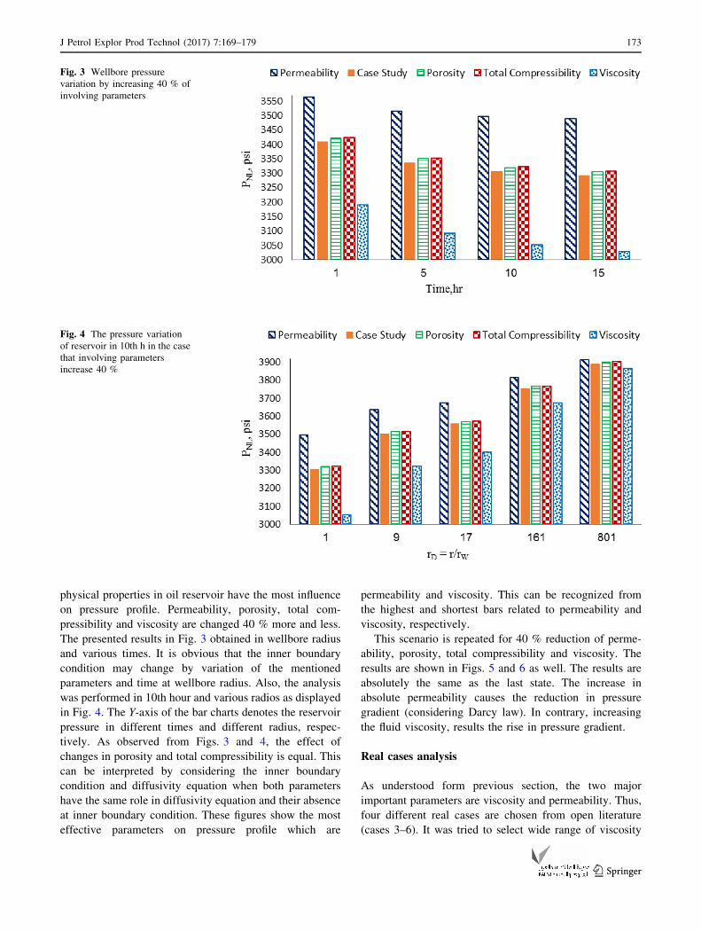
physical properties in oil reservoir have the most influence

on pressure profile. Permeability, porosity, total com-

pressibility and viscosity are changed 40 % more and less.

The presented results in Fig. 3 obtained in wellbore radius

and various times. It is obvious that the inner boundary

condition may change by variation of the mentioned

parameters and time at wellbore radius. Also, the analysis

was performed in 10th hour and various radios as displayed

in Fig. 4. The Y-axis of the bar charts denotes the reservoir

pressure in different times and different radius, respec-

tively. As observed from Figs. 3 and 4, the effect of

changes in porosity and total compressibility is equal. This

can be interpreted by considering the inner boundary

condition and diffusivity equation when both parameters

have the same role in diffusivity equation and their absence

at inner boundary condition. These figures show the most

effective parameters on pressure profile which are

permeability and viscosity. This can be recognized from

the highest and shortest bars related to permeability and

viscosity, respectively.

This scenario is repeated for 40 % reduction of perme-

ability, porosity, total compressibility and viscosity. The

results are shown in Figs. 5 and 6 as well. The results are

absolutely the same as the last state. The increase in

absolute permeability causes the reduction in pressure

gradient (considering Darcy law). In contrary, increasing

the fluid viscosity, results the rise in pressure gradient.

Real cases analysis

As understood form previous section, the two major

important parameters are viscosity and permeability. Thus,

four different real cases are chosen from open literature

(cases 3–6). It was tried to select wide range of viscosity

Fig. 3 Wellbore pressure

variation by increasing 40 % of

involving parameters

Fig. 4 The pressure variation

of reservoir in 10th h in the case

that involving parameters

increase 40 %

J Petrol Explor Prod Technol (2017) 7:169–179 173

123

and permeability for the chosen cases. Therefore, both light

and heavy oil along with low and high permeable rock used

in analysis are described in Table 1. L and H denote light

and heavy for oil and low and high for permeability,

respectively (Ahmed 2011; Craft et al. 1959; Torabi et al.

2016; Xu et al. 2016).

To evaluate other important parameters which poten-

tially may affect the pressure differences of linear and non-

linear diffusivity equation, the changes of production rate,

depletion time and radius are explored for the aforemen-

tioned cases. Figures 7 and 8 show the pressure differences

considering the variation of time, production rate and

reservoir radius. As seen, each case has different behavior

with respect to time, flow rate and radius changes. The

severest changes belong to case 6 (heavy oil and high

permeability), whereas the least important changes are

those of case 3 (light oil and low permeability). In addition,

the pressure differences increase by growing the depletion

time, production rate and decreasing reservoir radius.

Simultaneous changes of radius, depletion time and pro-

duction rate are considered to find the significant pressure

differences for each of 4 cases. In the present paper, critical

pressure (Pc) difference is arbitrarily set to 5 psi, and

pressure differences higher than 5 psi are considered to be

significant, as defined by Eq. (8).

Dpc ¼ pL � pNLj j ¼ 5psi ð8Þ

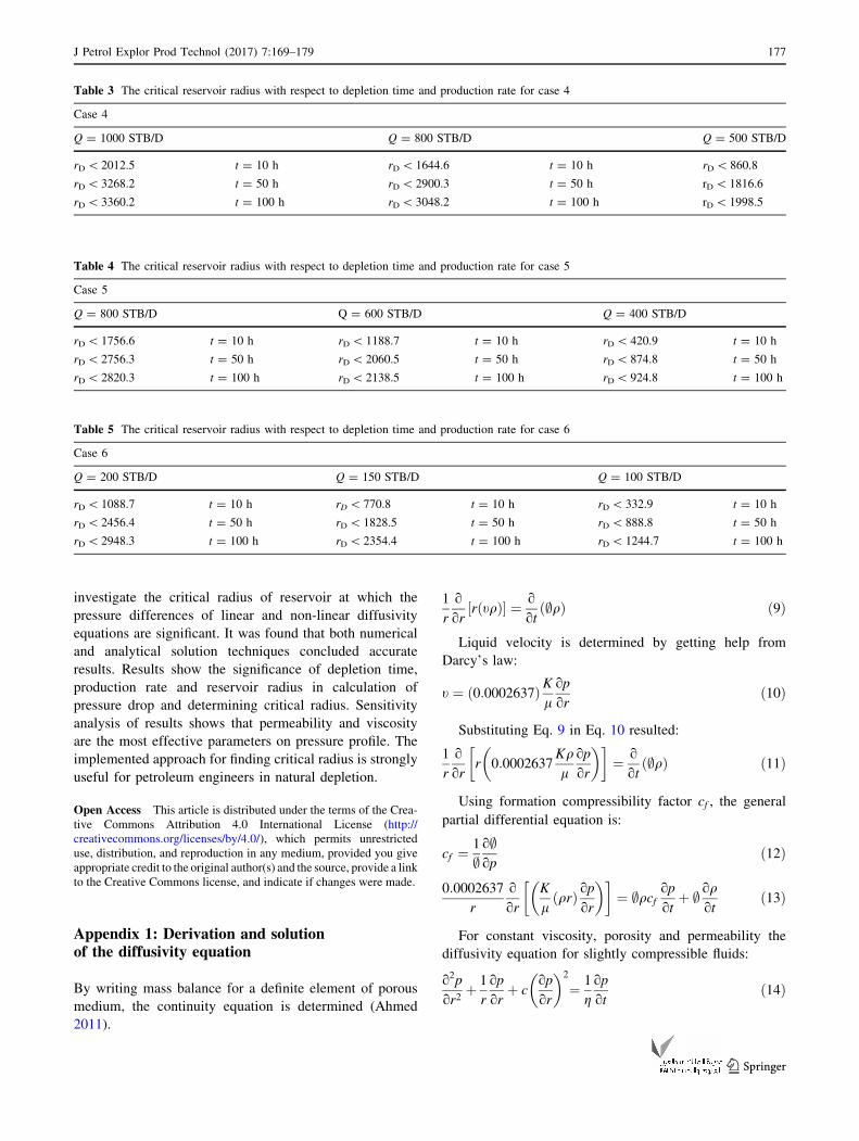
The reservoir radiuses in which the pressure differences

are thought to be critical are reported in Tables 2, 3, 4 and

5. These critical radiuses vary by changing depletion time

and production rate as observed in these tables. Beyond

that radius, pressure difference between linear and non-

linear becomes less than DPc, and both linear and non-

linear solutions apply with negligible error.

It should be taken into account that, by analyzing the

obtained results it was understood that, for the production

rates less than 500, 200, 230, 50 STB/day for each case

respectively, the pressure differences were not significant

Fig. 5 Wellbore pressure

variation by reducing 40 % of

involving parameters

Fig. 6 The pressure variation

of reservoir in 10th hr in the

case of 40 % parameters

decrease

174 J Petrol Explor Prod Technol (2017) 7:169–179

123

at all. This shows the significance of production rate at

which for every depletion time and reservoir radius the

pressure difference was insignificant. To put it another

way, while the flow rates of each cases are under the

boundary values, the pressure differences are less than

critical and unimportant. To clarify the presented issue, the

critical flow rates with variation of time and reservoir

radius are determined by nodes in Figs. 7 and 8. As seen in

Fig. 7, the pressure differences are highly significant for

presented case 6 where the flow rates are higher than

50 STB/day. On the other side, there is no critical flow rate

for case 3 regarding the smaller flow in compare with

500 STB/day index. Also, the indicated nodes on plotted

curve of cases 4 and 5 show the range of flow rates at

wellbore radius at which pressure differences are critical or

not. The similar scenario was repeated in Fig. 8, in which

the pressure differences were determined versus flow rates

for 10th and various radiuses. As observed from Fig. 8, the

designated nodes on curves of cases 4 and 5 belonging to

state A (wellbore radius) determine the border of critical

pressure. Whereas, the pressure differences of cases 3 and

6 are unimportant and highly critical, respectively. As

shown in Fig. 8, the pressure differences become unim-

portant for further distances. Hence, the pressure differ-

ences of other states (B–D) for each flow rates are normal

and unimportant as radius is extended.

Fig. 7 Comparison between different flow rates and depletion times considering in wellbore radius. a t = 10 h; b t = 30 h; c t = 50 h;

d t = 70 h

J Petrol Explor Prod Technol (2017) 7:169–179 175

123

Conclusion

In this work, a parametric analysis was studied on pressure

diffusivity equation. Results of numerical and analytical

solutions for both linear and non-linear pressure diffusivity

equations was presented and discussed. The critical radius

of reservoir, defined as the maximum radius of a reservoir

with certain rock and fluid properties in which the pressure

differences resulted from linear and non-linear solutions is

considerable, was used to analyze the results. Moreover,

four different cases including light and heavy oil along

with low and high permeable rock used in the analysis to

Fig. 8 Comparison between different flow rates and radiuses at t = 10 h. a r = rw; b r = 30.2 Ft; c r = 430.2 Ft; d r = 800.1 Ft

Table 2 The critical reservoir radius with respect to depletion time and production rate for case 3

Case 3

Q = 1200 STB/D Q = 1000 STB/D Q = 800 STB/D

rD\ 791.85 t = 10 h rD\ 504.4 t = 10 h rD = 215.2 t = 10 h

rD\ 1546.9 t = 50 h rD\ 1081.1 t = 50 h rD = 516.9 t = 50 h

rD\ 1654.1 t = 100 h rD\ 1163.2 t = 100 h rD = 574.1 t = 100 h

176 J Petrol Explor Prod Technol (2017) 7:169–179

123

investigate the critical radius of reservoir at which the

pressure differences of linear and non-linear diffusivity

equations are significant. It was found that both numerical

and analytical solution techniques concluded accurate

results. Results show the significance of depletion time,

production rate and reservoir radius in calculation of

pressure drop and determining critical radius. Sensitivity

analysis of results shows that permeability and viscosity

are the most effective parameters on pressure profile. The

implemented approach for finding critical radius is strongly

useful for petroleum engineers in natural depletion.

Open Access This article is distributed under the terms of the Crea-

tive Commons Attribution 4.0 International License (http://

creativecommons.org/licenses/by/4.0/), which permits unrestricted

use, distribution, and reproduction in any medium, provided you give

appropriate credit to the original author(s) and the source, provide a link

to the Creative Commons license, and indicate if changes were made.

Appendix 1: Derivation and solutionof the diffusivity equation

By writing mass balance for a definite element of porous

medium, the continuity equation is determined (Ahmed

2011).

1

r

o

orr tqð Þ½ � ¼ o

ot;qð Þ ð9Þ

Liquid velocity is determined by getting help from

Darcy’s law:

t ¼ 0:0002637ð ÞKlop

orð10Þ

Substituting Eq. 9 in Eq. 10 resulted:

1

r

o

orr 0:0002637

Kql

op

or

� �� �¼ o

ot;qð Þ ð11Þ

Using formation compressibility factor cf , the general

partial differential equation is:

cf ¼1

;o;op

ð12Þ

0:0002637

r

o

or

K

lqrð Þ op

or

� �� �¼ ;qcf

op

otþ ; oq

otð13Þ

For constant viscosity, porosity and permeability the

diffusivity equation for slightly compressible fluids:

o2p

or2þ 1

r

op

orþ c

op

or

� �2

¼ 1

gop

otð14Þ

Table 3 The critical reservoir radius with respect to depletion time and production rate for case 4

Case 4

Q = 1000 STB/D Q = 800 STB/D Q = 500 STB/D

rD\ 2012.5 t = 10 h rD\ 1644.6 t = 10 h rD\ 860.8

rD\ 3268.2 t = 50 h rD\ 2900.3 t = 50 h rD\ 1816.6

rD\ 3360.2 t = 100 h rD\ 3048.2 t = 100 h rD\ 1998.5

Table 4 The critical reservoir radius with respect to depletion time and production rate for case 5

Case 5

Q = 800 STB/D Q = 600 STB/D Q = 400 STB/D

rD\ 1756.6 t = 10 h rD\ 1188.7 t = 10 h rD\ 420.9 t = 10 h

rD\ 2756.3 t = 50 h rD\ 2060.5 t = 50 h rD\ 874.8 t = 50 h

rD\ 2820.3 t = 100 h rD\ 2138.5 t = 100 h rD\ 924.8 t = 100 h

Table 5 The critical reservoir radius with respect to depletion time and production rate for case 6

Case 6

Q = 200 STB/D Q = 150 STB/D Q = 100 STB/D

rD\ 1088.7 t = 10 h rD\ 770.8 t = 10 h rD\ 332.9 t = 10 h

rD\ 2456.4 t = 50 h rD\ 1828.5 t = 50 h rD\ 888.8 t = 50 h

rD\ 2948.3 t = 100 h rD\ 2354.4 t = 100 h rD\ 1244.7 t = 100 h

J Petrol Explor Prod Technol (2017) 7:169–179 177

123

c ¼ 1

qoqop

ð15Þ

g ¼ 0:0002637K

/lCt

ð16Þ

where c is the compressibility factor of slightly com-

pressible fluid.

Appendix 2: Analytical solution for linear and non-linear diffusivity equation and errors

The analytical solution of linear pressure diffusivity

equation concluded to Ei function (Ahmed 2011):

P r; tð Þ ¼ Pi þ70:6Q0lB0

Kh

� �Ei �x½ � ð17Þ

x ¼ 948;lctr2Kt

ð18Þ

where B0 is the formation volume factor.

The mathematical function of Ei is called exponential

integral (Ahmed 2011):

Ei �x½ � ¼ �Z1

x

e�udu

u¼ ln x� x

1!þ x2

2 2!ð Þ �x3

3 3!ð Þ

� �ð19Þ

For the values of x less than 0.01, the below

approximation is applicable:

Ei �x½ � ¼ ln 1:781xð Þ ð20Þ

And for range of x between 0.01 and 3:

Ei �x½ � ¼ a1 þ a2 ln xð Þ þ a3½ln xð Þ�2 þ a4 ln xð Þ½ �3þ a5x

þ a6x2 þ a7x

3 þ a8

x

ð21Þa1 ¼ �0:33153973 a2 ¼ �0:81512322a3 ¼ 5:22123384� 10�2 a4 ¼ 5:9849819� 10�3

a5 ¼ 0:662318450 a6 ¼ �0:12333524a7 ¼ 1:0832566� 10�2 a8 ¼ 8:6709776� 10�4

For most applicable ranges, there are some useful

figures in which the value of Ei can be determined knowing

x (Ahmed 2011).

The analytical solution of non-linear diffusivity equation

needs changing variables to perform linear equation to be

solved analytically (Odeh and Babu 1988).

o2p

or2þ 1

r

op

orþ c

op

or

� �2

¼ ;lckt

op

otð22Þ

Dp ¼ p� pi; T ¼ Kt

;lc andDp ¼ 1

cln p�

The linearized form is presented as:

o2p�

or2þ 1

r

op�

or¼ op�

oTð23Þ

The linear equation can be solved using Laplace

transform and concludes:

Dp ¼ �1

c

� �ln 1þ k ln

T

r2w

� �þ 0:2319

� �� ��

þ 0:5772k

1þ k ln Tr2w

þ 0:2319� �

1A ð24Þ

k ¼ qlc4pKh

where h is the formation thickness.

References

Ahmed T, McKinney P (2011) Advanced reservoir engineering. Gulf

Professional Publishing, Oxford

Braeuning S, Jelmert TA, Vik SA (1998) The effect of the quadratic

gradient term on variable-rate well-tests. J Petrol Sci Eng

21(3):203–222

Chakrabarty C, Ali S, Tortike W (1993) Analytical solutions for

radial pressure distribution including the effects of the quadratic-

gradient term. Water Resour Res 29(4):1171–1177

Craft BC, Hawkins MF, Terry RE (1959) Applied petroleum reservoir

engineering, vol 199. Prentice-Hall, Englewood Cliffs

Dake LP (1983) Fundamentals of reservoir engineering. Elsevier,

Amsterdam

Danesh A (1998) PVT and phase behaviour of petroleum reservoir

fluids, vol 47. Elsevier, Amsterdam

Eymard R, Sonier F (1994) Mathematical and numerical properties of

control-volumel finite-element scheme for reservoir simulation.

SPE Reserv Eng 9(04):283–289

Goode P (1987) Pressure drawdown and buildup analysis of horizontal

wells in anisotropic media. SPE Form Eval 2(04):683–697

Jelmert T, Vik S (1996) Analytic solution to the non-linear diffusion

equation for fluids of constant compressibility. J Petrol Sci Eng

14(3):231–233

Lee WJ (1992) Pressure transient testing: part 9. production

engineering methods. In: Development Geology Reference

Manual. AAPG Methods in Exploration No. 10, Tulsa, OK,

pp 477–481

Lee WJ, Wattenbarger RA (1996) Gas reservoir engineering, SPE

Textbook Series, Vol. 5.Society of Petroleum Engineers, p 349

Liang Y et al (2001) Nonlinear pressure diffusion in a porous

medium: approximate solutions with applications to permeabil-

ity measurements using transient pulse decay method. J Geophys

Res Solid Earth 106(B1):529–535

Loucks T, Guerrero E (1961) Pressure drop in a composite reservoir.

Soc Petrol Eng J 1(03):170–176

Marshall SL (2009) Nonlinear pressure diffusion in flow of

compressible liquids through porous media. Transp Porous

178 J Petrol Explor Prod Technol (2017) 7:169–179

123

Media 77(3):431–446

Odeh A, Babu D (1988) Comparison of solutions of the nonlinear and

linearized diffusion equations. SPE Reserv Eng 3(04):1202–1206

Torabi F, Mosavat N, Zarivnyy O (2016) Predicting heavy oil/water

relative permeability using modified Corey-based correlations.

Fuel 163:196–204

Van Everdingen A (1953) The skin effect and its influence on the

productive capacity of a well. J Petrol Technol 5(06):171–176

Van Everdingen A, Hurst W (1949) The application of the Laplace

transformation to flow problems in reservoirs. J Petrol Technol

1(12):305–324

Wang Y, Dusseault MB (1991) The effect of quadratic gradient terms

on the borehole solution in poroelastic media. Water Resour Res

27(12):3215–3223

Xu J et al (2016) Study on relative permeability characteristics

affected by displacement pressure gradient: experimental study

and numerical simulation. Fuel 163:314–323

Xu-long C, Deng-ke T, Rui-he W (2004) Exact solutions for nonlinear

transient flow model including a quadratic gradient term. Appl

Math Mech 25(1):102–109

J Petrol Explor Prod Technol (2017) 7:169–179 179

123