Parameterization Improvements and Functional and ...

Journal of Advances in Modeling Earth Systems – Discussion

Parameterization Improvements and Functional and Structural Advances in Version 4 of the Community Land Model

David M. Lawrence1, Keith W. Oleson1, Mark G. Flanner2, Peter E. Thornton3, Sean C. Swenson1, Peter J. Lawrence1, Xubin Zeng4, Zong-Liang Yang5, Samuel Levis1, Koichi Sakaguchi4, Gordon B. Bonan1, and Andrew G. Slater6

1 NCAR Earth System Laboratory, Climate and Global Dynamics Division, National Center for Atmospheric

Research, Boulder, CO, USA 2 Department of Atmospheric, Oceanic, and Space Sciences, University of Michigan, Ann Arbor, MI, USA 3 Environmental Sciences Division, Oak Ridge National Laboratory, Oak Ridge, TN, USA 4 Department of Atmospheric Sciences, University of Arizona, Tuscon, AZ, USA 5 Department of Geological Sciences, John A. and Katherine G. Jackson School of Geosciences, University of Texas

at Austin, Austin, TX, USA 6Cooperative Institute for Research in Environmental Sciences, University of Colorado, Boulder, CO, USA Manuscript submitted 14 May 2010, Revised 27 August, 2010, Accepted December 8, 2010 The Community Land Model is the land component of the Community Climate System Model. Here, we describe a broad set of model improvements and additions that have been provided through the CLM development community to create CLM4. The model is extended with a carbon-nitrogen (CN) biogeochemical model that is prognostic with respect to vegetation, litter, and soil carbon and nitrogen states and vegetation phenology. An urban canyon model is added and a transient land cover and land use change (LCLUC) capability, including wood harvest, is introduced, enabling study of historic and future LCLUC on energy, water, momentum, carbon, and nitrogen fluxes. The hy-drology scheme is modified with a revised numerical solution of the Richards equation and a revised ground evapo-ration parameterization that accounts for litter and within-canopy stability. The new snow model incorporates the SNow and Ice Aerosol Radiation model (SNICAR) - which includes aerosol deposition, grain-size dependent snow aging, and vertically-resolved snowpack heating – as well as new snow cover and snow burial fraction parameteri-zations. The thermal and hydrologic properties of organic soil are accounted for and the ground column is extended to ~50-m depth. Several other minor modifications to the land surface types dataset, grass and crop optical proper-ties, surface layer thickness, roughness length and displacement height, and the disposition of snow-capped runoff are also incorporated.

The new model exhibits higher snow cover, cooler soil temperatures in organic-rich soils, greater global river discharge, and lower albedos over forests and grasslands, all of which are improvements compared to CLM3.5. When CLM4 is run with CN, the mean biogeophysical simulation is degraded because the vegetation structure is prognostic rather than prescribed, though running in this mode also allows more complex terrestrial interactions with climate and climate change.

1. Introduction

Global models of the terrestrial surface continue to increase in complexity and accuracy as a result of improving existing process representations while also incorporating new processes and functionality

(see Pitman 2003). These models are used to gain understanding as to how land processes and anth-ropogenically or naturally evolving land states af-fect and interact with weather, climate, and cli-mate change. The Community Land Model (CLM, www.cesm.ucar.edu/models/cesm1.0/clm/)

2 Lawrence et al.

JAMES-D

is one of several global land models and is the land component used in the Community Climate Sys-tem Model (CCSM) (Collins et al. 2006b; Gent et al. 2009). Biogeophysical processes simulated by CLM include solar and longwave radiation inte-ractions with vegetation canopy and soil, momen-tum and turbulent fluxes from canopy and soil, heat transfer in soil and snow, hydrology of cano-py, soil, and snow, and stomatal physiology and photosynthesis. The CLM and the CCSM are community-developed models of the land and global climate systems and are used for studies of interannual and interdecadal variability, paleocli-mate regimes, and projections of future climate change. As a community model, CLM benefits from continual and extensive evaluation, criticism, and improvement by CLM users and developers.

The latest version of CLM, CLM4, builds on CLM3.5 (Oleson et al. 2008c) and is the result of a concerted effort by a diverse group of collabora-tors to address model deficiencies and biases and to add scientific capability to the model. CLM4 represents a significant advance in terrestrial mod-eling in the CCSM system. Changes to the model parameterizations and structure are extensive and include updates to soil hydrology, soil thermody-namics, the snow model, albedo parameters, the land surface types dataset, and the River Transport Model, as well as several other minor modifica-tions. The model has been extended with a carbon and nitrogen cycle model that includes prognostic vegetation phenology, the capability to apply tran-sient land cover and land use change, and a new urban canyon model that permits the study of the impact of climate change in urban areas and the urban heat island. Improvements to the way the offline forcing data (i.e. observed meteorological forcing) is applied across the diurnal cycle and to the partitioning of solar radiation into direct versus diffuse radiation have also been included in CLM4.

Many of the improvements adopted in CLM4 were developed independently by individual re-search groups for disparate reasons and applica-tions; therefore, one of the primary purposes of this paper is to catalog and describe the complete set of improvements (Section 2) and to character-ize their integrated impact on the performance of the model, primarily from the biogeophysical

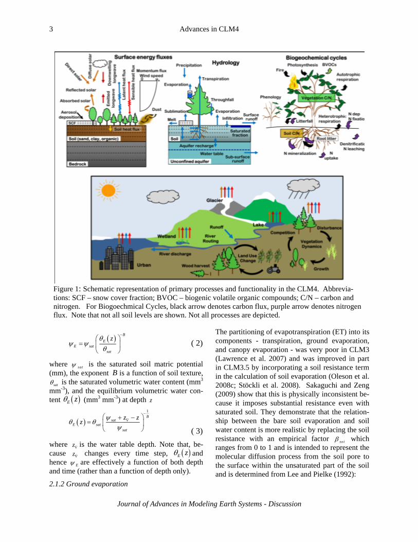
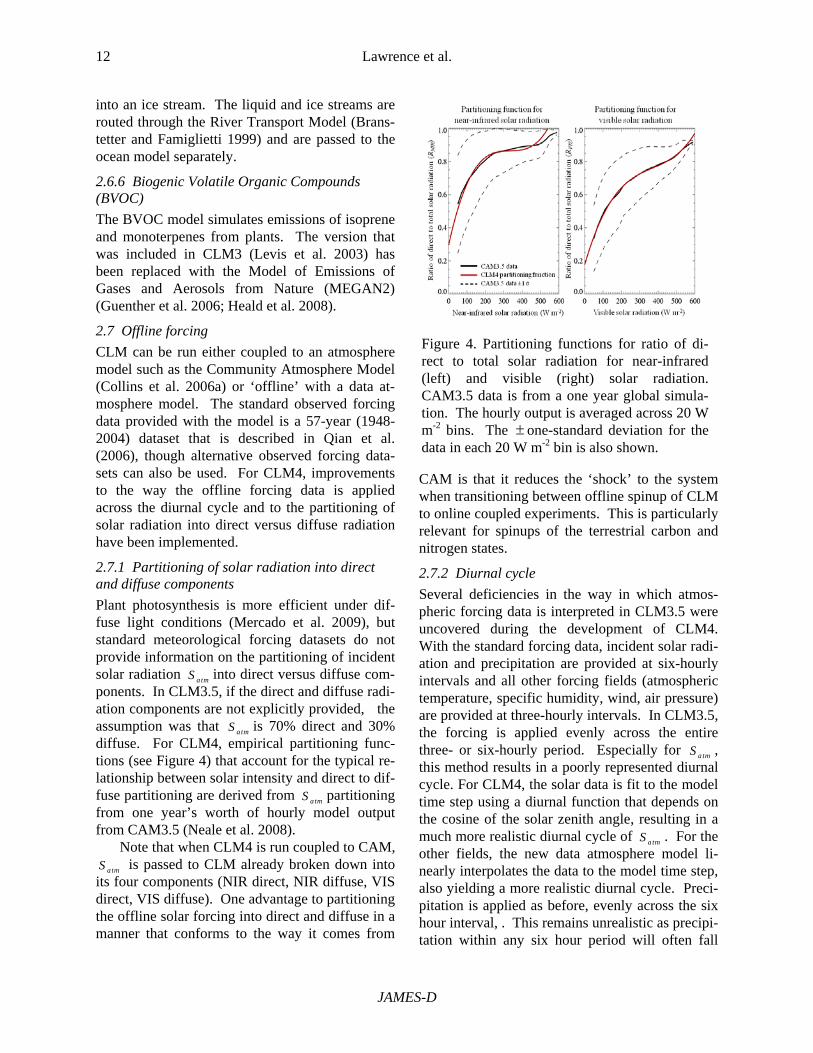
perspective, in offline simulations (Section 3). More detailed descriptions of the parameteriza-tions, and assessments of their performance in iso-lation, can be found in the cited papers. Compre-hensive documentation of the structure and algo-rithms used in CLM4 can be found in the CLM4.0 Technical Description (www.cesm.ucar.edu/models/cesm1.0/clm/CLM4_Tech_Note.pdf; Oleson et al. 2010). For refer-ence, we include a schematic diagram that depicts the main processes and functionality that exist in CLM4 (Figure 1).

2. Model improvements

2.1. Soil model

2.1.1 Richards equation

Zeng and Decker (2009) and Decker and Zeng (2009) demonstrate that the -based form of the Richards equation that governs vertical soil water movement and that is used in CLM3.5 cannot maintain the hydrostatic equilibrium soil moisture distribution because of truncation errors of the fi-nite-difference numerical scheme. The mass-conservative numerical scheme is deficient, espe-cially when the water table is within the soil col-umn, and these deficiencies cannot be resolved by increasing the vertical resolution of the soil col-umn. The solution is to explicitly subtract the hy-drostatic equilibrium soil moisture distribution, resulting in a modified Richards equation, as de-rived in Zeng and Decker (2009):

Ek Qt z z

( 1)

where is the volumetric soil water content (mm3 of water mm-3 of soil), k is the hydraulic conduc-tivity (mm s-1 ), is the soil matric potential (mm), E is the equilibrium soil matric potential (mm), and Q is a soil moisture sink term representing soil water losses due to transpiration (mm of water mm-1 of soil s-1). This equilibrium distribution can be derived at each time step from a constant hydraulic (i.e., capillary plus gravita-tional) potential above the water table, representing a steady-state solution of the Richards equation. The equilibrium soil matric potential is

3 Advances in CLM4

Journal of Advances in Modeling Earth Systems - Discussion

B

EE sat

sat

z

( 2)

where sat is the saturated soil matric potential (mm), the exponent B is a function of soil texture,

sat is the saturated volumetric water content (mm3 mm-3), and the equilibrium volumetric water con-tent E z (mm3 mm-3) at depth z

1

Bsat

E satsat

z zz

( 3)

where z is the water table depth. Note that, be-cause z changes every time step, E z and hence E are effectively a function of both depth and time (rather than a function of depth only).

2.1.2 Ground evaporation

The partitioning of evapotranspiration (ET) into its components - transpiration, ground evaporation, and canopy evaporation - was very poor in CLM3 (Lawrence et al. 2007) and was improved in part in CLM3.5 by incorporating a soil resistance term in the calculation of soil evaporation (Oleson et al. 2008c; Stöckli et al. 2008). Sakaguchi and Zeng (2009) show that this is physically inconsistent be-cause it imposes substantial resistance even with saturated soil. They demonstrate that the relation-ship between the bare soil evaporation and soil water content is more realistic by replacing the soil resistance with an empirical factor soi which ranges from 0 to 1 and is intended to represent the molecular diffusion process from the soil pore to the surface within the unsaturated part of the soil and is determined from Lee and Pielke (1992):

Figure 1: Schematic representation of primary processes and functionality in the CLM4. Abbrevia-tions: SCF – snow cover fraction; BVOC – biogenic volatile organic compounds; C/N – carbon and nitrogen. For Biogoechmical Cycles, black arrow denotes carbon flux, purple arrow denotes nitrogen flux. Note that not all soil levels are shown. Not all processes are depicted.

4 Lawrence et al.

JAMES-D

1 ,1

2

11 ,1

,1

1 or 0

0.25 1 *

1 cos

fc atm g

soi sno

fc snofc

q q

f

f

( 4)

where 1 and ,1fc are the volumetric liquid water content and field capacity of the top soil layer (m3 m-3) and snof is the fraction of ground covered by snow.

Sakaguchi and Zeng (2009) argue that, over regions with wetter soils, it is typically not the soil water content but rather the surface litter and the stable under-canopy air that controls ground eva-poration. Following their suggestions, for vege-tated surfaces, , the new soil evaporation function is

soi s g

g atm

aw litter

q qE

r r

. ( 5)

where sq and gq are the specific humidity of the canopy air and the soil surface (kg kg-1), atm is the density of atmospheric air (kg m-3), '

awr is the aerodynamic resistance (s m-1) to water vapor transfer between the ground and the canopy air. The litter resistance litterr (s m-1) is

11

0.004

efflitterL

litterr eu

( 6)

where the effective litter area index efflitterL (m2 m-2)

is the fraction of plant litter area index litterL (cur-rently set to 0.5 m2 m-2) that is not covered by snow and *u is the friction velocity (m s-1). In the future litterL is a parameter that could be prognosti-cally calculated by the model. The aerodynamic resistance 'awr is a function of the turbulent trans-fer coefficient sC which in CLM3.5 is a weighted combination of values for dense canopy Cs,dense and bare soil Cs,bare (Zeng et al. 2005). Instead of set-ting Cs,dense to the constant value of 0.004, as is done in CLM3.5, in CLM4

,

0.004 0

0.0040

1 min ,10

s g

s dense

s g

T T

CT T

S

( 7)

where sT and gT are canopy air and ground tem-

peratures, respectively and 0.5 and S is a sta-bility parameter that is a function of sT , gT , *u , and canopy top height. Combined, the new vege-tated and non-vegetated soil evaporation formula-tions exhibit higher gE at high latitudes and simi-lar or slightly higher gE in dry regions. A larger reduction of gE is found over regions with wet soil and more vegetation, leading to a better agreement with observations and independent modeling studies of the gE contribution to ET (Grelle et al. 1997; Choudhury et al. 1998; Bar-bour et al. 2005).

2.1.3 Thermal and hydrologic properties of organ-ic soil

Organic matter alters the thermal and hydraulic properties of soil. It acts as an insulator, with its low thermal conductivity and high heat capacity modulating the transfer of energy down into the soil during spring and summer and out of the soil during fall and winter, typically leading to cooler soil temperatures than would be apparent for pure mineral soils (Bonan and Shugart 1989). Organic or peat soils are also characterized by high porosi-ty, much higher than that of mineral soils, and cor-respondingly high hydraulic conductivity and weak soil suction. A global soil carbon dataset (GlobalSoilDataTask 2000) is used to build a geo-graphically distributed, vertically-profiled soil carbon density dataset applicable in CLM. In CLM3.5, soil properties such as thermal conduc-tivity and hydraulic conductivity are defined ac-cording to empirical relationships with soil texture (i.e., sand, silt, and clay contents; Oleson et al. 2004). In CLM4, soil physical properties are as-sumed to be a weighted combination of values for mineral soil and values for pure organic soil (Law-rence and Slater 2008). For example, the volume-tric water content at saturation (porosity) is now defined as

, , ,min, , ,(1 )sat i om i sat i om i sat omf f ( 8)

where , , ,max/om i om i omf , ,om i is the organic mat-ter density for layer i obtained from the CLM or-ganic matter dataset, ,maxom = 130 kg m-3 is the as-sumed density of pure organic soil, ,min,sat i is the porosity of mineral soil, and ,sat om = 0.9 is the po-rosity of organic matter. Parameters for thermal conductivity, heat capacity, saturated hydraulic

5 Advances in CLM4


conductivity, and soil water retention are similarly treated. Lawrence and Slater (2008) find that an-nual mean soil temperature in locations characte-rized by high organic matter content (e.g., northern high-latitudes) are cooled by up to ~2.5°C. Cool-ing is strongest in summer due to a reduction of early and mid-summer heat flux into the soil. High porosity and hydraulic conductivity of organic soil leads to a wetter soil column by volume but with comparatively low surface layer saturation levels and correspondingly reduced ground evaporation.

2.1.4 Soil/ground depth

Nicolsky et al. (2007) and Alexeev et al. (2007) demonstrated that soil temperature dynamics can-not be accurately modeled with a shallow soil col-umn and that a ground depth of at least 30m is re-quired for century-scale integrations. Therefore, in order to account for the thermal inertia of deep ground, the number of ground layers is extended in CLM4 from 10 to 15 layers, as in Lawrence et al. (2008). Layer thicknesses exponentially in-crease with depth, as before, ranging from a thick-ness of 0.018m at the surface to 13.9m for layer 15. The upper 10 layers are hydrologically active (i.e. the ‘soil’ layers) while the bottom five layers (3.8 m to 42 m depth) are thermal slabs that are not hydrologically active. The thermal conductivi-ty for the deep ground layers is set at 3.0 W m-1 K-1, which is comparable to that reported for satu-rated granitic rock (Clauser and Huenges 1995), while the heat capacity is set to that of a generic rock (2x106 J m-3 K-1) . The continued assumption of a globally uniform 3.8 m of hydrologically ac-tive soil remains unrealistic and is a deficiency of the model that requires attention in future devel-opment of the model.

2.1.5 Simplified bottom boundary condition for soil water equations

In CLM3.5, the redistribution of water within the soil column/aquifer system takes place in two steps. In the first step, the soil hydrology equa-tions are solved for the 10-layer soil column. Then, if the water table is deeper than the lowest soil layer, the aquifer recharge rate from the low-est soil layer to the unconfined aquifer is calcu-lated. This two-step procedure decouples the water fluxes within the soil column from the flux of wa-ter between the lowest layer and the aquifer layer,

leading on occasion to unrealistically large aquifer recharge rates.

For CLM4, the aquifer is coupled directly to the soil column via the soil water equations, result-ing in consistent moisture fluxes in the soil column / aquifer system. When the water table is within the soil column, a zero-flux boundary condition is applied at the bottom of the tenth layer, as in CLM3.5. When the water table drops from the lowest soil layer into the aquifer, an additional layer representing the portion of the aquifer be-tween the bottom of the lowest layer and the water table is added to the system of soil water equa-tions. The zero-flux boundary condition is then applied at the water table depth, rather than the bottom of the tenth layer.

2.1.6 Surface and subsurface runoff

Surface runoff in CLM3.5 and CLM4 consists of overland flow due to saturation excess (Dunne ru-noff) and infiltration excess (Hortonian runoff) mechanisms. The saturation excess term is a func-tion of the saturated fraction satf of the soil column, which includes a dependence on the surface layer frozen soil impermeable area fraction ,1frzf (Niu and Yang 2006) :

,1 max ,1(1 ) exp( 0.5 )sat frz over frzf f f f z f ( 9)

where maxf is the maximum saturated fraction, z is the water table depth, and overf is a decay factor. Subsurface runoff draiq is calculated according to the following expression (Niu et al. 2005):

,max(1 ) exp( )drai imp drai draiq f q f z ( 10)

where im pf is the fraction of impermeable area de-

termined from the ice content of the soil at depth, z is the water table depth, and draif is a decay factor. For CLM4, the decay factor overf and the maximum drainage ,maxdraiq when the water table is at the surface are adjusted through sensitivity analysis and comparison with observed runoff (

2.5overf in CLM3.5, 0.5overf in CLM4; ,maxdraiq = 4.5x10-4 kg m-2 s-1 in CLM3.5, ,maxdraiq = 5.5x10-3 kg m-2 s-1 in CLM4). The changes in these para-meters help alleviate the wet soil bias detected in CLM3.5 (Oleson et al. 2008c) and shifts the per-centages of surface runoff and subsurface runoff from 30%:70% to 55%:45%.

2.2. Snow model

6 Lawrence et al.

JAMES-D

2.2.1 SNICAR

The CLM3 snowpack radiation formulation is re-placed with SNICAR (SNow and ICe Aerosol Radiation; (Flanner and Zender 2005; Flanner and Zender 2006; Flanner et al. 2007)). In CLM3.5, new snow albedos are prescribed and snow albe-dos evolve according to a simple snow aging pa-rameterization (Oleson et al. 2004) and all solar radiation is absorbed in the up to 2-cm thick up-permost snow layer. SNICAR incorporates a two-stream radiative transfer solution based on Toon et al. (1989). Snow albedo and the vertical absorp-tion profile depend on solar zenith angle, the albe-do of the substrate underlying snow, mass concen-trations of atmospheric-deposited aerosols (black carbon, mineral dust, and organic carbon), and the ice effective grain size (re), which is simulated with a snow aging routine.

The two-stream solution produces upward and downward radiative fluxes at each snow layer in-terface, from which net radiation, layer absorption, and surface albedo are derived. Because snow al-bedo varies strongly across the solar spectrum, so-lar fluxes are computed in five spectral bands: four near-infrared bands (NIR) and one visible band. Incoming NIR radiation is split into the four NIR bands according to pre-defined weights for the di-rect and diffuse beams (see Table 3.4, Oleson et al. 2010). With ground albedo as a lower boundary condition, SNICAR simulates solar absorption in all snow layers as well as the underlyingground. Solar radiation penetration is limited to snowpacks with total snow depth greater than 0.1 m to prevent unrealistic soil warming within a single timestep.

The change in effective grain size is represented in each snow layer as a summation of changes caused by dry snow metamorphism, liq-uid water-induced metamorphism, refreezing of liquid water, and addition of freshly-fallen snow. The mass of each snow layer is partitioned into fractions of snow carrying over from the previous timestep, freshly-fallen snow, and refrozen liquid water. Dry snow metamorphism is based on a mi-crophysical model described by Flanner and Zend-

er (2006). This model simulates diffusive vapor flux amongst collections of ice crystals with vari-ous size and inter-particle spacing. Specific sur-face area and effective radius are prognosed for any combination of snow temperature, temperature gradient, density, and initial size distribution. The combination of warm snow, large temperature gradient, and low density produces the most rapid snow aging, whereas aging proceeds slowly in cold snow, regardless of temperature gradient and density.

SNICAR requires atmospheric deposition rates for the following eight particle species: hy-drophilic black carbon, hydrophobic black carbon, hydrophilic organic carbon, hydrophobic organic carbon, and four species of mineral dust. Each of these species has unique optical properties and meltwater removal efficiencies. In offline CLM simulations (and coupled simulations without prognostic aerosols), aerosol deposition rates are prescribed according to rates obtained from a tran-sient 1850-2009 CAM-chem (1.9° latitude by 2.5° longitude) simulation with interactive chemistry (troposphere and stratosphere). This simulation was driven by CCSM3 20th century sea-surface temperatures and emissions for short-lived gases and aerosols; observed concentrations were speci-fied for methane, nitrous oxide, the ozone-depleting substances (CFCs) and CO2 (Lamarque et al. 2010).

Overall, snow albedo, solar absorption, and aging processes interact with each other in a more physically-based manner in SNICAR. Fresh snow is brighter resulting in slightly brighter albedos over Antarctica and Greenland. Snow aging oc-curs more slowly, especially in cold regions, and exhibits greater spread across different snow tem-perature regimes. SNICAR darkens the snow in areas that receive large amounts of black carbon and/or dust deposition (e.g., east Asia, Tibetan Plateau, central and eastern Europe, and eastern North America).

2.2.2 Snow cover fraction

7 Advances in CLM4


Ground albedo is a weighted average of snow-covered and snow-free albedos, where the weight-ing is determined by the snow cover fraction, snof . For CLM4, we replace the snof parameterization with a density-dependent parameterization derived by Niu and Yang (2007). The new formulation takes the following form:

0,

tanh2.5 ( / )

snosno m

g sno new

zf

z

( 11)

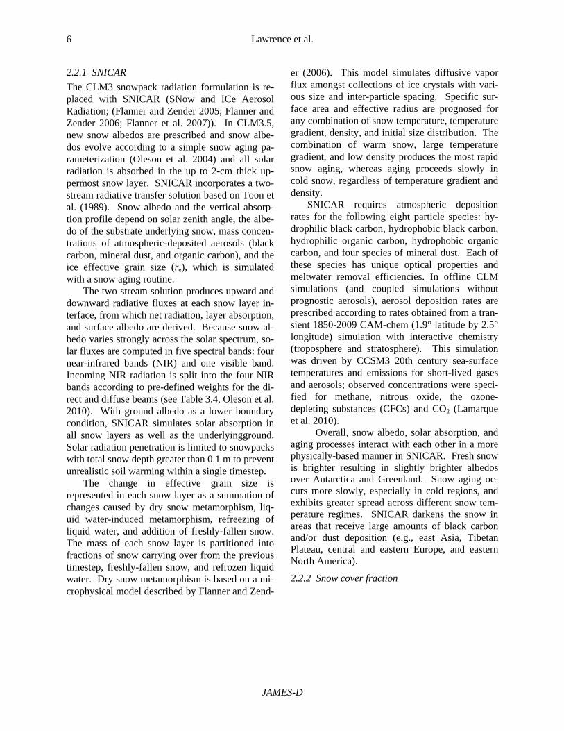
where snoz is the snow depth, 0 , gz is the roughness length of bare soil sno is the prognostic bulk den-sity of the snowpack and 100new kg m-3 is the density of new snow, and m = 1 is a scale-dependent melting factor that can be calibrated against observed snof . The new formulation in-creases snof by about 20-50% depending on loca-tion and time of year, resulting in much better agreement with observed snof Figure 2). The im-pact is especially pronounced at relatively shallow snow depths. The density-dependent formulation accounts for the observation that there is a sharper rise in snof with snow depth early in the snow sea-son (e.g., October, November, and December), when snowpack density is comparatively low than

there is during the warmer melt season (e.g., March, April, and May) when the snowpack is comparatively dense (see Figure 2, Niu and Yang 2007).

2.2.3 Burial fraction of vegetation by snow

The vertical fraction of vegetation buried by snow sno

vegf is used to determine the exposed leaf and stem area indices. In CLM3.5, all plant functional types (PFTs) utilize the same parameterization for

snovegf that is a function of snow depth as well as ca-

nopy top and canopy bottom heights. Based on the work of Wang and Zeng (2009), the sno

vegf para-meterization is updated in CLM4 to treat tall vege-tation (tree and shrub) and short vegetation (grass and crops) separately according to

for trees and shrubs

min , for grasses and crops

sno sno botveg

top bot

sno csnoveg

c

z zf

z z

z zf

z

( 12)

where topz and botz are PFT-specific canopy top and bottom heights that are either prescribed or prognostic (i.e., they are prognostic when the car-bon-nitrogen cycle model is active, see Section

Figure 2. Maps of climatological annual mean (1985-2004) snow cover fraction for CLM3.5 and CLM4SP (where SP stands for the CLM4 version with prescribed climatological satellite phenology, see Section 2.3) versus observations (for years 1967-2003) for the Northern hemisphere. Observed snow cover fraction is derived from National Oceanic and Atmospheric Administration AVHRR data (Robinson and Frei 2000).

8 Lawrence et al.

JAMES-D

2.3) and cz = 0.2 m is the critical snow depth at which short vegetation is assumed to be complete-ly buried by snow. This modification largely eli-minates unrealistic surface turbulent fluxes that occur during snowmelt and leads to a more realis-tic timing and rate of snowmelt.

2.2.4 Other snow modifications

Minor errors in the calculation of snow compac-tion rates and in the vertical snow temperature pro-file during layer splitting were corrected (Law-rence and Slater 2009). These two corrections re-sult in a 5-10% reduction in the simulated annual maximum snow depths and eliminate unrealistic snow and soil temperature perturbations that occur immediately after a snow layer splitting event. Another minor error was corrected to ensure that snow enthalpy is always conserved during snow layer combination.

2.3 Carbon and nitrogen biogeochemistry

The model is extended with a carbon-nitrogen (CN) biogeochemical model (Thornton et al. 2007; Randerson et al. 2009; Thornton et al. 2009). CN is based on the terrestrial biogeochemistry Biome-BGC model (Thornton et al. 2002; Thornton and Rosenbloom 2005). It is prognostic with respect to carbon and nitrogen state variables in vegeta-tion, litter, and soil organic matter. CLM4 can be run with or without an active CN model. When CN is inactive, leaf area and stem area indices (LAI, SAI), and vegetation heights are prescribed according to data derived from MODIS (see Sec-tion 2.6.2, we refer to this mode as CLM4SP where SP stands for satellite phenology). When CN is active, LAI, SAI, and vegetation heights are determined prognostically by the model (hereafter CLM4CN). When the carbon-nitrogen biogeo-chemistry is active (CLM4CN), potential gross primary production (GPP) is calculated from leaf photosynthetic rate without nitrogen constraint. The nitrogen required to achieve this potential GPP is diagnosed, and the actual GPP is decreased for nitrogen limitation. In CLM4SP, this potential GPP must be reduced by multiplying the photo-synthetic parameter Vcmax (maximum rate of car-boxylation) by a PFT-specific factor scaled be-tween zero and one that represents nitrogen con-straints on GPP. The nitrogen factors were derived from CLM4CN simulations (see Oleson et al.

2008c).

2.3.1 Prognostic vegetation phenology

The CLM4CN phenology model consists of sever-al algorithms, operating at seasonal timescales. Three distinct phenological types are represented by separate algorithms: evergreen, seasonal-deciduous, and stress-deciduous. These are intro-duced briefly below.

Within the evergreen phenology algorithm, lit-terfall is specified to occur only through the back-ground litterfall mechanism – there are no distinct periods of litterfall for evergreen types, but rather a continuous (slow) shedding of foliage and fine roots. The rate of background litterfall depends on a specified leaf longevity. The seasonal-deciduous phenology algorithm is based on the parameteriza-tions for leaf onset and offset for temperate deci-duous broadleaf forest (White et al. 1997; Thorn-ton et al. 2002). Initiation of leaf onset is triggered when a common degree-day summation exceeds a critical value, and leaf litterfall is initiated when daylength is shorter than a critical value. The stress-deciduous phenology algorithm has been developed specifically for CLM4CN, but it is based in part on the grass phenology model pro-posed by White et al. (1997). The algorithm han-dles phenology for vegetation types such as grasses and tropical drought-deciduous trees that respond to both cold and drought-stress signals, and that can have multiple growing seasons per year. The algorithm also allows for the possibility that leaves might persist year-round in the absence of a suitable stress trigger. In that case the phenol-ogy switches to an evergreen habit, maintaining a marginally-deciduous leaf longevity (one year) un-til the occurrence of the next stress trigger. In rel-atively warm climates, onset triggering depends solely on soil water availability, whereas in cold climates onset triggering depends on both accumu-lated soil temperature summation and adequate soil moisture. Any one of three conditions is suf-ficient to trigger the initiation of an offset period: sustained period of dry soil, sustained period of cold temperature, or daylength shorter than 6 hours.

2.3.2 Dynamic vegetation (CNDV)

The dynamic global vegetation model that was available in prior versions of CLM (CLM-dgvm;

9 Advances in CLM4


Levis et al. 2004) has been integrated with CN to form CLM4CNDV which is an optional mode for CLM4. In CNDV, the annual processes of light competition, establishment, and survival as they pertain to the calculations of PFT cover and popu-lation are retained from CLM-DGVM. Except for the background mortality rate, for which the CLM-DGVM algorithms are retained, all other ecosys-tem processes (allocation, phenology, fire, etc.) are now handled by CN. CLM-dgvm only considered grass and tree PFTs; CLM4CNDV has been ex-tended to also include a shrub PFT (Zeng et al. 2008). CLM4CNDV simulations are not pre-sented in this paper.

2.4 Urban model

A parameterization for urban surfaces has been developed and incorporated into CLM4 (Oleson et al. 2008a; Oleson et al. 2008b). At the global scale, and at the coarse spatial resolution of the CCSM, urbanization has negligible impact on cli-mate. However, the urban parameterization, CLMU, allows simulation of the urban environ-ment within a climate model, and particularly the air temperature and humidity where the majority of people work and live. As such, the urban model allows scientific study of how climate change af-fects the urban heat island and possible urban planning and design strategies to mitigate warm-ing.

The urban system is represented as separate landunit within the grid cell and is based upon the “urban canyon” concept of Oke (1987) in which the canyon geometry is described by building height and street width. The canyon system con-sists of roofs, walls, and canyon floor. Walls are further divided into shaded and sunlit components. The canyon floor is divided into pervious (e.g., to represent residential lawns, parks) and impervious (e.g., to represent roads, parking lots, sidewalks) fractions.

Applications of the model make use of data-sets of urban extent, morphology (e.g., height to width ratio, roof fraction, average building height, and pervious fraction of the canyon floor), and ra-diative (e.g., albedo and emissivity) and thermal (e.g., heat capacity and thermal conductivity) properties of urban materials developed by Jack-son et al. (2010).

2.5 Transient land cover and land use change

New in CLM4 is the capability to prescribe tran-sient land cover and land use change (LCLUC). The LCLUC dataset used in CLM4 derives from a global historical transient land use and land cover change dataset, namely Version 1 of the Land-Use History A product (LUHa.v1, (Hurtt et al. 2006), referred to here as the UNH dataset) covering the period 1850-2005. The UNH dataset, available at 0.5° resolution, describes land cover and its change via four classes of vegetation: crop, pas-ture, primary vegetation, and secondary vegeta-tion. A transition matrix is provided with the LULC datasets that describes the annual fraction of land that is transformed from one category to another (e.g., primary land to crop, pasture to crop, etc.). Included in these transitions is the ‘conver-sion’ of secondary land to secondary land, repre-senting logging on previously disturbed land.

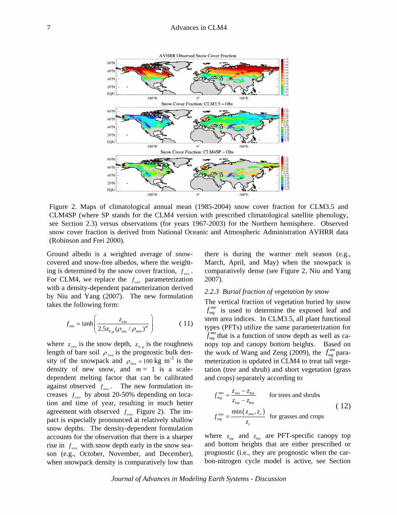
The information in the LCLUC datasets is then translated across to CLM’s PFT distribution in four steps, resulting in an annual gridded time series of PFT weights. First, crop PFT composi-tion is directly specified from the crop land unit fractional area. Second, pasture PFTs are assigned based on grass PFTs found in the potential vegeta-tion and current day CLM land surface parameters scaled by the area of pasture. Third, potential ve-getation PFTs are assigned to the grid cell scaled by the fractional area of the primary land unit. Last, current day non-crop and non-pasture PFTs are assigned to the grid cell scaled by the fraction-al area of the secondary land unit. The annual tree harvest values also are calculated from the harvest information of the UNH dataset used in conjunc-tion with transient tree PFT values. Separate data-sets representing the extent of water, wetland, ice and urban land cover are used to compile the final land cover present in each CLM grid cell. These additional non-vegetated land cover fractions are held constant throughout the time series. The present day dataset is based on the methodology in Lawrence and Chase (2007, see Section 2.6.2) and the potential vegetation is derived as in Lawrence and Chase (2010). Figure 3 shows the CLM4 PFT distributions according to the major classes of ve-getation (trees, shrubs, grasses, and crops) for the year 2000 and the difference relative to potential vegetation (year 1850).

10 Lawrence et al.

JAMES-D

Changes in PFT fractional cover over time are incorporated during a simulation via interpolation of PFT weights between annual time slices for year a and year b using a simple linear algorithm. This linear algorithm is applied at each timestep throughout a year such that the PFT weights for year b are realized exactly at the beginning of year b. Mass and energy are conserved through PFT weight changes through checks on total water and heat content before and after a transition. Any small discrepancy in water or energy due to chang-ing PFT weights is accounted for in runoff or in

the sensible heat flux.

2.6 Other modifications

2.6.1 Land surface types dataset

The PFT distribution is re-derived from multi-year Moderate Resolution Imaging Spectroradiometer (MODIS, Justice et al. 2002; Hansen et al. 2003) land surface data products and is as in CLM3.5 (Lawrence and Chase 2007) except that a new cropping dataset is used (Ramankutty et al. 2008) and a high grass PFT fraction bias in forested re-gions has been alleviated by replacing understory

Figure 3. Maps of PFT distribution, collated from the 16 CLM PFTs into trees, shrubs, grasses, and crops for the year 2000 and the change in PFT distribution since the year 1850.

11 Advances in CLM4


grasses reported in the MODIS data with short trees (see Figure 3 for tree, shrub, grass, and crop distribution in CLM4). This change results in im-proved grid cell mean albedos and leaf area indic-es when compared to MODIS data. Globally, the present day vegetation distribution (for non-glacier, non-lake, non-wetland, non-urban land area) shifts from 25% bare ground, 23% tree, 11% shrub, 31% grass, and 11% crop in the CLM3.5 land surface types dataset to 25% bare ground, 39% tree, 8% shrub, 20% grass, and 9% crop in CLM4. Soil colors are re-derived by the same protocol as in Lawrence and Chase (2007), but with the updated vegetation maps. Lake and wet-land areal fractions in the CLM3.5 surface dataset were derived from MODIS land cover data which were subsequently found to be unrealistically low. For CLM4, the lake and wetland distributions re-vert back to those used in CLM3 (Cogley 1991), except that the threshold area fraction that is used to determine whether or not a lake, wetland, or glacier surface type is represented in a particular grid cell is reduced from 5% to 1%. In CLM3.5, only the four most dominant PFTs are represented in any grid cell. For CLM4, partly to accommo-date requirements of transient land cover change, this restriction is relaxed such that all PFTs with non-zero grid cell MODIS area fractions are represented.

2.6.2 Grass and crop optical properties

Analysis of albedos simulated in CLM3.5 indi-cated that grassland and cropland albedos generat-ed with the optical properties taken from Dorman and Sellers (1989) are unrealistically high. Leaf and stem optical properties for grasses and crops are updated with values calculated from full opti-cal range spectra of measured optical properties (Asner et al. 1998). For updated values see Table 3.1 in the CLM4 Tech Note (Oleson et al. 2010).

2.6.3 Surface layer thickness

In prior versions of CLM, the sensible heat, latent heat, and momentum fluxes are determined for the surface layer between the surface at height 0z dand the atmospheric reference height, where 0z is roughness length (m) and d is displacement height (m). The atmospheric reference height is assumed to be the height above the ground. Since

0z and d vary depending on the type of surface

and there may be multiple surface types within a grid cell, the surface fluxes were determined for different surface layer thicknesses. In CLM4, the atmospheric reference height is now assumed to be the height above 0z d , thereby ensuring that the fluxes are consistently determined over the same surface layer thickness for all surface types. More importantly, the atmospheric reference height is no longer constrained to be greater than 0z d , which allows for a thin lowest atmospheric model layer.

2.6.4 Roughness length and displacement height for sparse and dense canopies

The vegetation displacement height and the roughness lengths are functions of plant height. The convergence of canopy roughness length (

, 0 , 0 ,, ,om v h v w vz z z ; momentum, sensible heat, water vapor, respectively) and displacement height ( d ) to bare soil values as the above-ground biomass goes to zero is ensured as in Zeng and Wang (2007) according to

0

0 , 0 , 0 ,

0 ,

lnexp

1 ln

top z m

m v h v w v

m g

V z Rz z z

V z

( 13)

top dd z R V ( 14)

where topz is canopy top height (m), 0z mR and dR are the ratio of momentum roughness length and displacement height to canopy top height, respec-tively, and 0 ,m gz is the ground momentum rough-ness length (m). The fractional weight V is de-termined from

1 exp min ,

1 exp

cr

cr

L S L SV

L S

( 15)

where =1 and crL S is a critical value of ex-

posed leaf plus stem area for which 0mz reaches its maximum. This change results in seasonal changes in sensible heat flux of 10 W m-2.

2.6.5 Liquid and ice water streams

To improve global energy conservation when CLM is being run as part of CCSM, runoff is split into two streams, a liquid water stream and an ice water stream. New snowfall that falls on snow-capped grid cells (to avoid continual accumulation of snow in very cold climates, the snowpack is capped at 1m snow water equivalent) is partitioned

12 Lawrence et al.

JAMES-D

into an ice stream. The liquid and ice streams are routed through the River Transport Model (Brans-tetter and Famiglietti 1999) and are passed to the ocean model separately.

2.6.6 Biogenic Volatile Organic Compounds (BVOC)

The BVOC model simulates emissions of isoprene and monoterpenes from plants. The version that was included in CLM3 (Levis et al. 2003) has been replaced with the Model of Emissions of Gases and Aerosols from Nature (MEGAN2) (Guenther et al. 2006; Heald et al. 2008).

2.7 Offline forcing

CLM can be run either coupled to an atmosphere model such as the Community Atmosphere Model (Collins et al. 2006a) or ‘offline’ with a data at-mosphere model. The standard observed forcing data provided with the model is a 57-year (1948-2004) dataset that is described in Qian et al. (2006), though alternative observed forcing data-sets can also be used. For CLM4, improvements to the way the offline forcing data is applied across the diurnal cycle and to the partitioning of solar radiation into direct versus diffuse radiation have been implemented.

2.7.1 Partitioning of solar radiation into direct and diffuse components

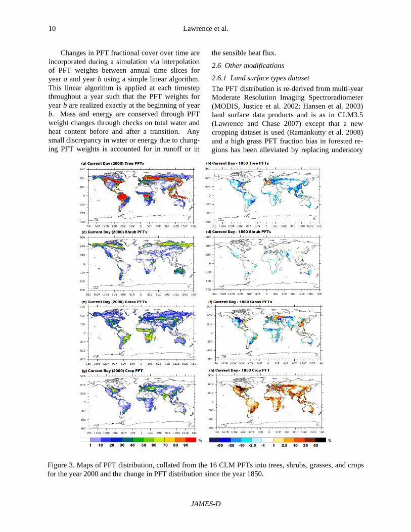
Plant photosynthesis is more efficient under dif-fuse light conditions (Mercado et al. 2009), but standard meteorological forcing datasets do not provide information on the partitioning of incident solar radiation atmS into direct versus diffuse com-ponents. In CLM3.5, if the direct and diffuse radi-ation components are not explicitly provided, the assumption was that atmS is 70% direct and 30% diffuse. For CLM4, empirical partitioning func-tions (see Figure 4) that account for the typical re-lationship between solar intensity and direct to dif-fuse partitioning are derived from atmS partitioning from one year’s worth of hourly model output from CAM3.5 (Neale et al. 2008).

Note that when CLM4 is run coupled to CAM,

atmS is passed to CLM already broken down into its four components (NIR direct, NIR diffuse, VIS direct, VIS diffuse). One advantage to partitioning the offline solar forcing into direct and diffuse in a manner that conforms to the way it comes from

CAM is that it reduces the ‘shock’ to the system when transitioning between offline spinup of CLM to online coupled experiments. This is particularly relevant for spinups of the terrestrial carbon and nitrogen states.

2.7.2 Diurnal cycle

Several deficiencies in the way in which atmos-pheric forcing data is interpreted in CLM3.5 were uncovered during the development of CLM4. With the standard forcing data, incident solar radi-ation and precipitation are provided at six-hourly intervals and all other forcing fields (atmospheric temperature, specific humidity, wind, air pressure) are provided at three-hourly intervals. In CLM3.5, the forcing is applied evenly across the entire three- or six-hourly period. Especially for atmS , this method results in a poorly represented diurnal cycle. For CLM4, the solar data is fit to the model time step using a diurnal function that depends on the cosine of the solar zenith angle, resulting in a much more realistic diurnal cycle of atmS . For the other fields, the new data atmosphere model li-nearly interpolates the data to the model time step, also yielding a more realistic diurnal cycle. Preci-pitation is applied as before, evenly across the six hour interval, . This remains unrealistic as precipi-tation within any six hour period will often fall

Figure 4. Partitioning functions for ratio of di-rect to total solar radiation for near-infrared (left) and visible (right) solar radiation. CAM3.5 data is from a one year global simula-tion. The hourly output is averaged across 20 W m-2 bins. The one-standard deviation for the data in each 20 W m-2 bin is also shown.

13 Advances in CLM4


over just one or two time steps. Qian et al., (2006) suggest that this problem can be reduced by ad-justing precipitation rates using observed precipi-tation frequency maps. However, sensitivity tests indicate that the runoff formulation currently im-plemented in CLM4 is not very sensitive to preci-pitation intensity. This is an aspect of the offline model that requires further investigation and in which the modeling system can be improved.

3. Simulations

Several offline simulations were completed to as-sess the integrated impact of the model improve-ments for difference configurations of the model and compared to CLM3.5. The model output data and meteorological forcing data for these simula-tions is available through the Earth System Grid (via www.cesm.ucar.edu/models/cesm1.0/clm). Four primary simulations are conducted: (1) CLM3.5 with the old data atmosphere forcing me-thod (CLM3.5OF), (2) CLM3.5 with the new forc-ing method (CLM3.5, see Section 2.7), (3) CLM4 with prescribed satellite-derived vegetation phe-nology (i.e., LAI, SAI, and vegetation height de-fined by satellite observations as in CLM3.5; CLM4SP), and (4) CLM4 with vegetation phenol-

ogy determined by the carbon-nitrogen biogeo-chemistry model (CLM4CN, see Section 2.3.1). In principle, CLM can be run at any resolution. These uncoupled simulations were conducted at a standard resolution for CLM4 and CCSM4 of 0.9° latitude by 1.25° longitude and were driven by a 57-year long (1948-2004) atmospheric forcing da-taset (Qian et al. 2006). Land state variables (e.g., soil temperature and moisture) for the CLM3.5OF and CLM3.5 simulations were spunup for 30 years with repeat year 1948 forcing while CLM4SP was spunup for an additional 120 years to account for the longer spinup timescale of the deep ground layers. The CLM3.5OF, CLM3.5, and CLM4SP simulations used static surface PFT distributions and aerosol deposition for the year 2000.

Two CLM4CN simulations were conducted. The first was initialized from a long (~1350 year) CLM4CN spinup simulation with repeat year 1948-1972 atmospheric forcing and 1850 PFT dis-tribution, CO2, nitrogen and aerosol deposition (the much longer spinup timescales for CLM4CN are dictated by the long timescales required to bring the carbon and nitrogen pools and associated LAI, SAI, and vegetation heights to approximate equilibrium). This spinup simulation is followed

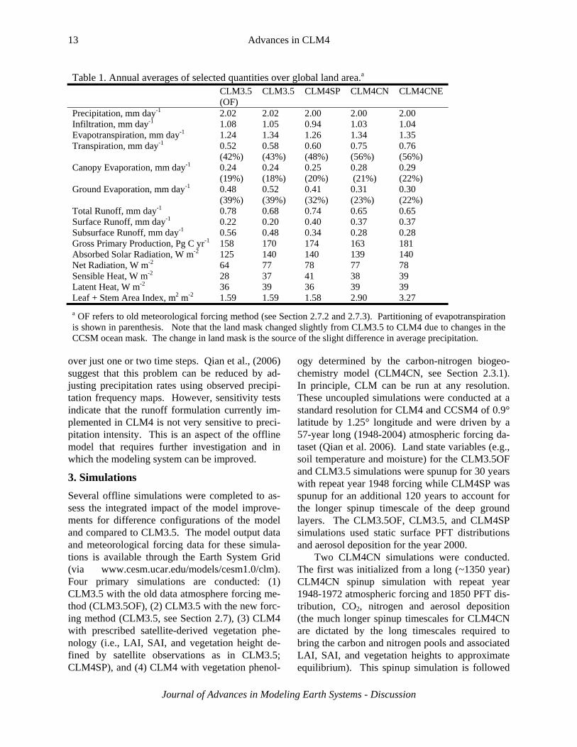
Table 1. Annual averages of selected quantities over global land area.a CLM3.5

(OF) CLM3.5 CLM4SP CLM4CN CLM4CNE

Precipitation, mm day-1 2.02 2.02 2.00 2.00 2.00 Infiltration, mm day-1 1.08 1.05 0.94 1.03 1.04 Evapotranspiration, mm day-1 1.24 1.34 1.26 1.34 1.35 Transpiration, mm day-1 0.52

(42%) 0.58 (43%)

0.60 (48%)

0.75 (56%)

0.76 (56%)

Canopy Evaporation, mm day-1 0.24 (19%)

0.24 (18%)

0.25 (20%)

0.28 (21%)

0.29 (22%)

Ground Evaporation, mm day-1 0.48 (39%)

0.52 (39%)

0.41 (32%)

0.31 (23%)

0.30 (22%)

Total Runoff, mm day-1 0.78 0.68 0.74 0.65 0.65 Surface Runoff, mm day-1 0.22 0.20 0.40 0.37 0.37 Subsurface Runoff, mm day-1 0.56 0.48 0.34 0.28 0.28 Gross Primary Production, Pg C yr-1 158 170 174 163 181 Absorbed Solar Radiation, W m-2 125 140 140 139 140 Net Radiation, W m-2 64 77 78 77 78 Sensible Heat, W m-2 28 37 41 38 39 Latent Heat, W m-2 36 39 36 39 39 Leaf + Stem Area Index, m2 m-2 1.59 1.59 1.58 2.90 3.27

a OF refers to old meteorological forcing method (see Section 2.7.2 and 2.7.3). Partitioning of evapotranspiration is shown in parenthesis. Note that the land mask changed slightly from CLM3.5 to CLM4 due to changes in the CCSM ocean mask. The change in land mask is the source of the slight difference in average precipitation.

14 Lawrence et al.

JAMES-D

by a 154 year transient simulation (1850-2004) in which the PFT distributions evolve according to the transient LCLUC dataset (see Section 2.5) and with prescribed transient CO2 and nitrogen deposi-tion rates (Lamarque et al. 2010). Aerosol deposi-tion rates were held constant at year 1850 levels. A second CLM4CN simulation was run out to equi-librium with PFT distributions, CO2, aerosol and nitrogen deposition data for the year 2000 with 1948-2004 atmospheric forcing (denoted CLM4CNE, Table 1).

4. Results

4.1. Impact of improved application of meteoro-logical forcing

Improving the diurnal cycle of incident solar rad-iation and incorporating an empirical partitioning of atmS into direct and diffuse radiation has a sig-

nificant impact on the offline model results. Global average values for selected model diagnos-tics are presented in Table 1. (CLM3.5 (OF) and CLM3.5). Absorbed solar radiation is significant-ly higher (+15 W m-2; net radiation, +13 W m-2) with the new forcing method since all the atmSprovided in the forcing dataset is forced to arrive during daylight timesteps see Section 2.7.2). The increase in absorbed solar radiation leads to in-creases in sensible heat flux (SH, +9 W m-2), latent heat flux (LH, +3 W m-2) and GPP (+12PgC yr-1). Approximately +6 PgC yr-1 of the GPP increase can be attributed to higher photosynthesis rates as-sociated with the improved partitioning of solar radiation into direct and diffuse components. The higher LH (i.e., evapotranspiration, ET) results in reduced runoff.

Figure 5. Climatological mean (1985-2004) annual cycle time series for Amazonia for selected va-riables. Albedo observations are from MODIS. Correlation of prescribed versus prognostic LAI across annual cycle shown for exposed LAI.

15 Advances in CLM4


4.2. Turbulent fluxes and ET Partitioning

4.2.1 Global simulations

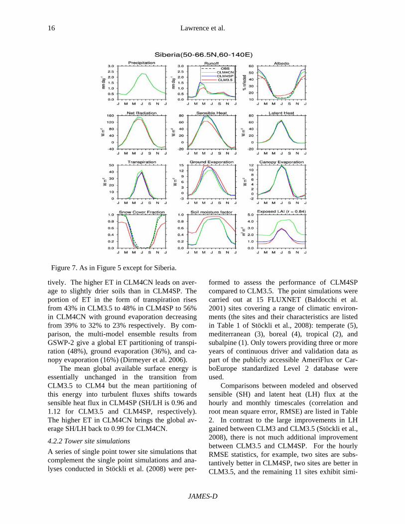
The combined impact of the suite of model changes described in Section 2 is illustrated via climatological annual cycle time series for three regions - Amazonia (Figure 5), the central United States (Figure 6), and Siberia (Figure 7) – which were subjectively selected to illustrate several as-pects of the new model. A robust change across all three regions is a decrease in ground evapora-tion. The decrease in ground evaporation is a re-sult of the new litter resistance function and the reduction of turbulent exchange under a dense ca-nopy with the new canopy turbulence formulation (Section 2.1.2). To meet atmospheric demand, the reduced ground evaporation is compensated for with increased transpiration, even though the on average drier soils increase soil moisture stress on vegetation (i.e., lower soil moisture factor in summer; note that the reduction in the soil mois-ture factor in Siberia in CLM4 is due to colder

soils resulting from the insulating properties of the organic-rich soil, see Section 4.6). Additional in-creases in transpiration and decreases in ground evaporation in CLM4CN are associated with the generally higher than observed LAI values simu-lated in these regions in CLM4CN.

Changes in the meridional distribution of ET and its partitioning are shown in Figure 8. A de-crease in ground evaporation at all latitudes is off-set somewhat by a slight rise in transpiration with canopy evaporation unchanged. Consequently, total ET is lower (and runoff is correspondingly higher, see Section 4.3) in CLM4SP compared to CLM3.5. In CLM4CN, higher LAI values trans-late into higher transpiration and slightly higher canopy evaporation and lower ground evaporation compared to CLM4SP. The increase in transpira-tion and canopy evaporation outweighs the de-crease in ground evaporation resulting in enhanced total ET at most latitudes. Globally, total ET shifts from 1.34 mm d-1 to 1.26 mm d-1 to 1.34 mm d-1 in CLM3.5, CLM4SP, and CLM4CN respec-

Figure 6. As in Figure 5 except for the Central US. Snow cover fraction observations are from AVHRR (Robinson and Frei 2000).

16 Lawrence et al.

JAMES-D

tively. The higher ET in CLM4CN leads on aver-age to slightly drier soils than in CLM4SP. The portion of ET in the form of transpiration rises from 43% in CLM3.5 to 48% in CLM4SP to 56% in CLM4CN with ground evaporation decreasing from 39% to 32% to 23% respectively. By com-parison, the multi-model ensemble results from GSWP-2 give a global ET partitioning of transpi-ration (48%), ground evaporation (36%), and ca-nopy evaporation (16%) (Dirmeyer et al. 2006).

The mean global available surface energy is essentially unchanged in the transition from CLM3.5 to CLM4 but the mean partitioning of this energy into turbulent fluxes shifts towards sensible heat flux in CLM4SP (SH/LH is 0.96 and 1.12 for CLM3.5 and CLM4SP, respectively). The higher ET in CLM4CN brings the global av-erage SH/LH back to 0.99 for CLM4CN.

4.2.2 Tower site simulations

A series of single point tower site simulations that complement the single point simulations and ana-lyses conducted in Stöckli et al. (2008) were per-

formed to assess the performance of CLM4SP compared to CLM3.5. The point simulations were carried out at 15 FLUXNET (Baldocchi et al. 2001) sites covering a range of climatic environ-ments (the sites and their characteristics are listed in Table 1 of Stöckli et al., 2008): temperate (5), mediterranean (3), boreal (4), tropical (2), and subalpine (1). Only towers providing three or more years of continuous driver and validation data as part of the publicly accessible AmeriFlux or Car-boEurope standardized Level 2 database were used.

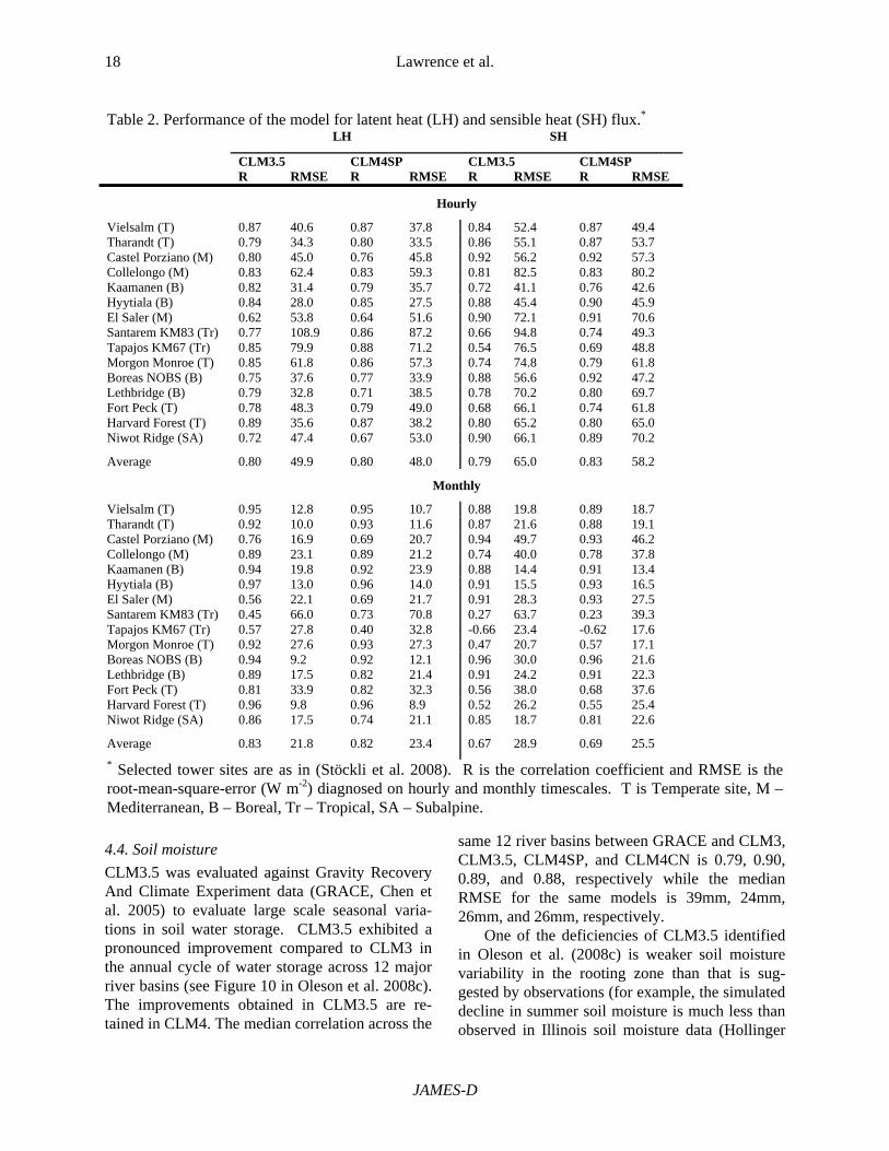
Comparisons between modeled and observed sensible (SH) and latent heat (LH) flux at the hourly and monthly timescales (correlation and root mean square error, RMSE) are listed in Table 2. In contrast to the large improvements in LH gained between CLM3 and CLM3.5 (Stöckli et al., 2008), there is not much additional improvement between CLM3.5 and CLM4SP. For the hourly RMSE statistics, for example, two sites are subs-tantively better in CLM4SP, two sites are better in CLM3.5, and the remaining 11 sites exhibit simi-

Figure 7. As in Figure 5 except for Siberia.

17 Advances in CLM4


lar performance in CLM3.5 and CLM4SP. For SH, there is a modest indication that CLM4SP is the superior model. For hourly RMSE, CLM4SP is the best model for four sites while the remaining 11 sites exhibit similar performance. Average hourly RMSE across all 15 drops from 65.0 W m-2 to 58.2 W m-2 from CLM3.5 to CLM4SP.

4.3. Runoff

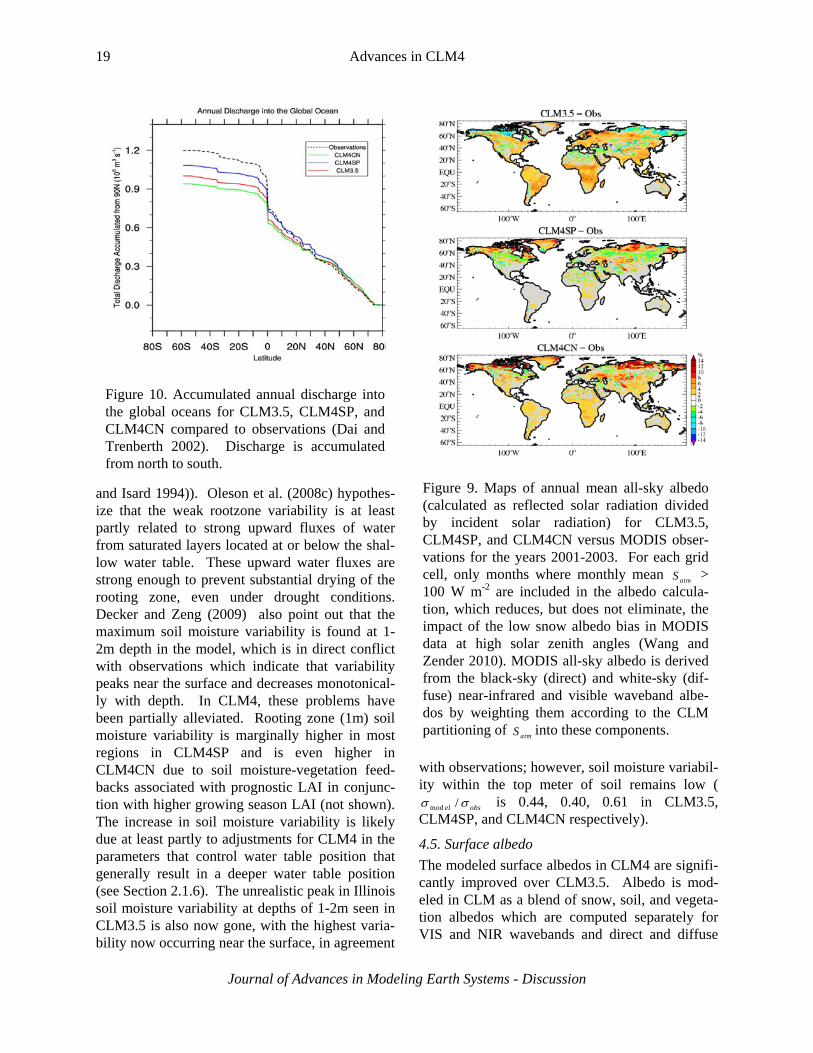
Total runoff increases by ~9% in CLM4SP over CLM3.5 (Table 2) resulting in better agreement with the observed annual discharge into the global oceans (Figure 10), though discharge remains ~9% too low in CLM4SP, which implies that global ET is too high. There is a significant shift towards the

fast component of runoff (surface) at the expense of the slow component (sub-surface), reversing in part the shift from CLM3 to CLM3.5 (Oleson et al. 2008c). The increase in surface runoff is pri-marily a function of the downward adjustment of the overf decay factor (see Section 2.1.6). At high latitudes, the increase in surface runoff is also a function of lower soil permeability associated with the cooler soil temperatures and increased ice frac-tions that are a result of representing the thermal properties of organic soil to the model (see Section 2.1.3 and Section 2.1.6). One outcome of this is an increase in runoff during the spring snowmelt season as less of the snow meltwater infiltrates in-to the soil (see regional Siberia plots, Figure 7) which leads to an improvement in the annual cycle of river discharge to the Arctic Ocean, which was acknowledged as a deficiency in CLM3.5 (Oleson et al. 2008c). We also compared against compo-site monthly climatological runoff data from the University of New Hampshire-Global Runoff Data Center (UNH-GRDC; Fekete et al. 2002), which was area-averaged from 0.5o to the model resolu-tion but masked by UNH-GRDC observed runoff fields. Globally, the climatological monthly RMSE against the UNH-GRDC data is only mar-ginally different, rising slightly from 0.78 mm day-

1 in CLM3.5 to 0.82 mm day-1 in CLM4SP. This increase in RMSE, while at the same time the total discharge bias goes down, suggests a slight degra-dation of the timing of runoff in CLM4SP relative to CLM3.5.

In CLM4CN runoff is significantly lower than in CLM4SP due to higher ET in CLM4CN. Glob-al annual discharge is lower than observations by ~23% in CLM4CN. The source of the lower dis-charge is predominantly low discharge levels from tropical rivers (Figure 10), which suggests that ET is too high in the tropics, especially the Amazon. Transpiration and canopy evaporation levels in the tropics are significantly higher in CLM4CN than in CLM4SP which can be attributed to high simu-lated LAI values in CLM4CN (see for example the regional Amazonia plots, Figure 5).

Figure 8. Zonal mean plots of total evapo-transpiration and its components for CLM4SP (top panel), CLM4SP minus CLM3.5 (middle panel), and CLM4CN minus CLM4SP (bottom panel). Zonal means are averaged over ~3° latitude bins to improve presentation clarity.

18 Lawrence et al.

JAMES-D

4.4. Soil moisture

CLM3.5 was evaluated against Gravity Recovery And Climate Experiment data (GRACE, Chen et al. 2005) to evaluate large scale seasonal varia-tions in soil water storage. CLM3.5 exhibited a pronounced improvement compared to CLM3 in the annual cycle of water storage across 12 major river basins (see Figure 10 in Oleson et al. 2008c). The improvements obtained in CLM3.5 are re-tained in CLM4. The median correlation across the

same 12 river basins between GRACE and CLM3, CLM3.5, CLM4SP, and CLM4CN is 0.79, 0.90, 0.89, and 0.88, respectively while the median RMSE for the same models is 39mm, 24mm, 26mm, and 26mm, respectively.

One of the deficiencies of CLM3.5 identified in Oleson et al. (2008c) is weaker soil moisture variability in the rooting zone than that is sug-gested by observations (for example, the simulated decline in summer soil moisture is much less than observed in Illinois soil moisture data (Hollinger

Table 2. Performance of the model for latent heat (LH) and sensible heat (SH) flux.* LH SH

CLM3.5 CLM4SP CLM3.5 CLM4SP R RMSE R RMSE R RMSE R RMSE

Hourly

Vielsalm (T) 0.87 40.6 0.87 37.8 0.84 52.4 0.87 49.4 Tharandt (T) 0.79 34.3 0.80 33.5 0.86 55.1 0.87 53.7 Castel Porziano (M) 0.80 45.0 0.76 45.8 0.92 56.2 0.92 57.3 Collelongo (M) 0.83 62.4 0.83 59.3 0.81 82.5 0.83 80.2 Kaamanen (B) 0.82 31.4 0.79 35.7 0.72 41.1 0.76 42.6 Hyytiala (B) 0.84 28.0 0.85 27.5 0.88 45.4 0.90 45.9 El Saler (M) 0.62 53.8 0.64 51.6 0.90 72.1 0.91 70.6 Santarem KM83 (Tr) 0.77 108.9 0.86 87.2 0.66 94.8 0.74 49.3 Tapajos KM67 (Tr) 0.85 79.9 0.88 71.2 0.54 76.5 0.69 48.8 Morgon Monroe (T) 0.85 61.8 0.86 57.3 0.74 74.8 0.79 61.8 Boreas NOBS (B) 0.75 37.6 0.77 33.9 0.88 56.6 0.92 47.2 Lethbridge (B) 0.79 32.8 0.71 38.5 0.78 70.2 0.80 69.7 Fort Peck (T) 0.78 48.3 0.79 49.0 0.68 66.1 0.74 61.8 Harvard Forest (T) 0.89 35.6 0.87 38.2 0.80 65.2 0.80 65.0 Niwot Ridge (SA) 0.72 47.4 0.67 53.0 0.90 66.1 0.89 70.2

Average 0.80 49.9 0.80 48.0 0.79 65.0 0.83 58.2

Monthly

Vielsalm (T) 0.95 12.8 0.95 10.7 0.88 19.8 0.89 18.7 Tharandt (T) 0.92 10.0 0.93 11.6 0.87 21.6 0.88 19.1 Castel Porziano (M) 0.76 16.9 0.69 20.7 0.94 49.7 0.93 46.2 Collelongo (M) 0.89 23.1 0.89 21.2 0.74 40.0 0.78 37.8 Kaamanen (B) 0.94 19.8 0.92 23.9 0.88 14.4 0.91 13.4 Hyytiala (B) 0.97 13.0 0.96 14.0 0.91 15.5 0.93 16.5 El Saler (M) 0.56 22.1 0.69 21.7 0.91 28.3 0.93 27.5 Santarem KM83 (Tr) 0.45 66.0 0.73 70.8 0.27 63.7 0.23 39.3 Tapajos KM67 (Tr) 0.57 27.8 0.40 32.8 -0.66 23.4 -0.62 17.6 Morgon Monroe (T) 0.92 27.6 0.93 27.3 0.47 20.7 0.57 17.1 Boreas NOBS (B) 0.94 9.2 0.92 12.1 0.96 30.0 0.96 21.6 Lethbridge (B) 0.89 17.5 0.82 21.4 0.91 24.2 0.91 22.3 Fort Peck (T) 0.81 33.9 0.82 32.3 0.56 38.0 0.68 37.6 Harvard Forest (T) 0.96 9.8 0.96 8.9 0.52 26.2 0.55 25.4 Niwot Ridge (SA) 0.86 17.5 0.74 21.1 0.85 18.7 0.81 22.6

Average 0.83 21.8 0.82 23.4 0.67 28.9 0.69 25.5

* Selected tower sites are as in (Stöckli et al. 2008). R is the correlation coefficient and RMSE is the root-mean-square-error (W m-2) diagnosed on hourly and monthly timescales. T is Temperate site, M – Mediterranean, B – Boreal, Tr – Tropical, SA – Subalpine.

19 Advances in CLM4


and Isard 1994)). Oleson et al. (2008c) hypothes-ize that the weak rootzone variability is at least partly related to strong upward fluxes of water from saturated layers located at or below the shal-low water table. These upward water fluxes are strong enough to prevent substantial drying of the rooting zone, even under drought conditions. Decker and Zeng (2009) also point out that the maximum soil moisture variability is found at 1-2m depth in the model, which is in direct conflict with observations which indicate that variability peaks near the surface and decreases monotonical-ly with depth. In CLM4, these problems have been partially alleviated. Rooting zone (1m) soil moisture variability is marginally higher in most regions in CLM4SP and is even higher in CLM4CN due to soil moisture-vegetation feed-backs associated with prognostic LAI in conjunc-tion with higher growing season LAI (not shown). The increase in soil moisture variability is likely due at least partly to adjustments for CLM4 in the parameters that control water table position that generally result in a deeper water table position (see Section 2.1.6). The unrealistic peak in Illinois soil moisture variability at depths of 1-2m seen in CLM3.5 is also now gone, with the highest varia-bility now occurring near the surface, in agreement

with observations; however, soil moisture variabil-ity within the top meter of soil remains low (

mod /el obs is 0.44, 0.40, 0.61 in CLM3.5, CLM4SP, and CLM4CN respectively).

4.5. Surface albedo

The modeled surface albedos in CLM4 are signifi-cantly improved over CLM3.5. Albedo is mod-eled in CLM as a blend of snow, soil, and vegeta-tion albedos which are computed separately for VIS and NIR wavebands and direct and diffuse

Figure 9. Maps of annual mean all-sky albedo (calculated as reflected solar radiation divided by incident solar radiation) for CLM3.5, CLM4SP, and CLM4CN versus MODIS obser-vations for the years 2001-2003. For each grid cell, only months where monthly mean atmS > 100 W m-2 are included in the albedo calcula-tion, which reduces, but does not eliminate, the impact of the low snow albedo bias in MODIS data at high solar zenith angles (Wang and Zender 2010). MODIS all-sky albedo is derived from the black-sky (direct) and white-sky (dif-fuse) near-infrared and visible waveband albe-dos by weighting them according to the CLM partitioning of atmS into these components.

Figure 10. Accumulated annual discharge into the global oceans for CLM3.5, CLM4SP, and CLM4CN compared to observations (Dai and Trenberth 2002). Discharge is accumulated from north to south.

20 Lawrence et al.

JAMES-D

radiation. Changes in modeled albedo are a com-bined result of the new surface dataset in which grass and shrub PFT fractions are generally lower in forested regions (Section 2.6.2), reduced grass and crop leaf and stem reflectance values (Section 2.6.1), and new snow cover fraction (Section 2.2.2) and snow burial fraction formulations (Sec-tion 2.2.3). The improvements in the simulated albedo are apparent in the three focal regions (Figure 5, Figure 6, Figure 7). For Amazonia, the annual mean albedo is clearly improved in CLM4SP, but the annual cycle is out of phase. Mean albedo in CLM4CN is biased high, despite the much larger LAI values, which a priori one would expect to decrease the albedo. The increase in albedo between CLM4CN and CLM4SP and the out of phase problem may both be related to the prescribed relationship between soil albedo and soil wetness (drier soils have higher soil albe-do). CLM4CN is slightly drier than CLM4SP in Amazonia due to high transpiration rates and the peak in albedo in CLM4SP occurs during the dry season. Both results suggest that the soil albedo-soil wetness relationship may be too strong or per-haps should not be invoked for tropical rainforests. For the central US, the positive influence of the adjusted grass/crop albedos (summer and early au-tumn) and the new snow cover fraction paramete-rization (snow season) are both apparent in the al-bedo plot (Figure 6, note the improvement in snow cover fraction).

Global maps of all-sky albedo bias compared to MODIS collection 4 estimates are shown in

Figure 9. The mean bias is reduced throughout the tropics and mid-latitudes. The bias across the bo-real forest regions shifts from positive to negative. Across the northern high latitudes, an opposite shift occurs with low albedos biases supplanted with high albedo biases. The MODIS snow albe-do retrievals appear to be biased significantly low at high solar zenith angles (Wang and Zender 2010), and therefore the model’s winter high-latitude (i.e., high solar zenith angle) bright albedo bias may not necessarily be indicative of a model deficiency. Note also that the excessively bright wintertime albedo in CLM4 over Siberia (Figure 7), despite a good simulation of snow cover frac-tion, is consistent with the assessment that MODIS snow albedo is biased low.

For the most part, CLM4CN albedo is similar to CLM4SP albedo, except in the northern high latitudes where CLM4CN albedos are slightly higher. This difference is probably due to the short vegetation heights simulated in very cold re-gions in CLM4CN (not shown), which leads to more frequent burial of vegetation by snow and consequently brighter albedos. Global area-weighted bias, RMSE, and pattern correlation sta-tistics are listed in Table 3. The mean albedo bias and RMSE decreases for snow-free points by 2.3% and 2.1%, respectively for CLM4SP compared to CLM3.5. For locations/months with snow cover, the mean bias swings from low to high (-5% to +2.9%), though for grid cells dominated by short vegetation (i.e. grasses and shrubs) the change is from a low bias (-12.5%) to a high bias (+5.6%)

Table 3. Global albedo statistics versus MODIS observation estimates.*

Bias (%) RMSE (%)

Model zsnow = 0.0m

zsnow > 0.2m

zsnow > 0.2m, grass+shrub > 75%

zsnow > 0.2m, tree > 75%

zsnow = 0.0m

zsnow > 0.2m

zsnow > 0.2m, grass+shrub > 75%

zsnow > 0.2m, tree > 75%

CLM3.5 2.7 -5.0 -12.5 2.4 4.1 11.9 16.7 6.2 CLM4SP 0.4 2.9 5.6 -7.9 2.0 13.2 12.3 10.2 CLM4CN 1.8 4.0 5.6 -4.8 2.9 14.8 17.6 9.5 * Area-weighted bias and RMSE for simulated versus observed albedo. The 2001-2003 CLM modeled climatol-ogy is compared to the 2001-2003 MODIS climatology. zsnow is snow depth. Results are calculated from monthly mean climatological values. Locations/months with atmS < 100 W m-2 and/or land fraction less than one (e.g. partial land / partial ocean grid cells) and glacier cells are excluded. Rightmost two columns for Bias and RMSE show results grid cells are screened for grass+shrub or tree dominance.

21 Advances in CLM4


while grid cells dominated by trees shift in the op-posite direction (2.4% to -7.9%). These vegetation type specific changes are consistent with the new snow burial fraction for short vegetation paramete-rization and the increase in forested area in CLM4.

4.6. Soil temperature / Permafrost

Soils are biased warm in northern high latitudes in CLM3.5, especially in summer at depth (Figure 11). This warm bias contributes to low simulated Northern Hemisphere near-surface permafrost ex-tent (8.2 million km2; we define near-surface permafrost extent in the model as the integrated area in which at least one soil layer within the up-permost 3.8m remains below 0oC throughout the year (Lawrence et al. 2008)). Observed estimates of Northern Hemisphere continuous permafrost (90–100% coverage) and discontinuous permafrost

(50–90% coverage) area combined are 11.8 – 14.7 million km2 (Zhang et al. 2000). Adding a repre-sentation of the thermal and hydrologic properties of organic soil (Section 2.1.3) and extending the ground column to ~50m (Section 2.1.4) in CLM3.5 (CLM3.5ORGDEEP) improved the simu-lation of northern high-latitude soil temperature considerably with the active layer depth (depth to which soils thaw in the summer) apparently well-simulated (see Figure 2, Lawrence et al. 2008). In CLM4, the northern high-latitude soils are even colder than they were in CLM3.5ORGDEEP and now appear to be biased low compared to the ob-served Siberian soil temperatures. Near-surface permafrost extent in CLM4 is now on the high end of the observed estimates (14.2 million km2 in CLM4SP). The cause of the decrease in soil tem-

Figure 11. Climatological (1985-2000) annual cycle-depth plots of soil temperature (filled contours) and percent saturation (lined contours, shown for model simulations only). Russian soil temperature monitor-ing data that spans most of Siberia (~900 sites; Zhang et al. 2001) was regridded to the CLM grid and then averaged across all grid cells that contain at least one permafrost (e.g. perennially frozen) ground layer within the upper 3.2 m of soil (126 grid cells). Equivalent grid cells extracted and averaged over the same time period for CLM simulations.

22 Lawrence et al.

JAMES-D

Figure 12. Change in variability of LE, SH, absorbed solar radiation, and LAI+SAI from CLM3.5 to CLM4SP (left panels) and CLM4SP to CLM4CN (right panels). Variability is calculated as the stan-dard deviation (ANN STDev) of the monthly 1948-2004 detrended anomaly time series.

perature between CLM3.5ORGDEEP and CLM4 may be related to changes in the hydrology para-meters that control water table position (Section 2.1.6). In CLM3.5ORGDEEP, locations with permafrost tended to exhibit nearly saturated soils throughout the soil column that were wetter than in CLM3.5 (see Figure 8, Lawrence and Slater 2008). In CLM4, the lower water table position allows the soils to dry out considerably resulting in very dry soils near the surface (Figure 11). The dry near-surface organic soils have very low ther-mal conductivity which restricts heat from pene-

trating into the soil during summer, leading to the cool soil temperatures and shallow active layer. Our hypothesis is that the soils are too dry, though soil moisture data that is co-located with the soil temperature data is not available to confirm or re-fute this hypothesis. However, other tertiary evi-dence also suggests that Arctic soil moisture may be biased low, including simulated area-averaged peak LAI in CLM4CN that is ~1 m2 m-2 too low (not shown). Sensitivity tests with a model ver-sion with wetter Arctic soils exhibit warmer soil temperatures and improved simulation of LAI in

23 Advances in CLM4


tundra regions. Cold region hydrology remains a weakness in the model and will be the subject of a follow-up study and future model development.

4.7. Variability

Changes in variability (defined here as the stan-dard deviation of monthly 1948-2004 detrended anomaly time series) for LH and SH, absorbed so-lar radiation, and LAI+SAI are shown in Figure 12 for CLM4SP – CLM3.5 and CLM4CN – CLM4SP. Considering first CLM4SP – CLM3.5, LH variability moderately increases in some arid and semi-arid regions, reflecting the drier soil conditions in CLM4SP and an associated increase in the frequency of moisture-limited evapotranspi-ration. Variability in absorbed solar radiation also increases in a few northern hemisphere locations, likely due to increased variation in the timing of snowmelt.

By contrast, in CLM4CN the variability in LH and SH increases by between 50 and 200% in CLM4CN across several regions including the central and eastern US, southeastern South Ameri-ca, southern Asia, and the Sahel. These regions coincide with regions of relatively strong LAI+SAI variability generated by the prognostic phenology model in CLM4CN. Inspection of the monthly annual cycle of LH and LAI+SAI stan-dard deviations for selected regions indicates that the variability increase is associated with both en-

hanced growing season LAI+SAI variability (e.g., central US) and by variations in the timing of leaf onset (e.g., India) and offset in CLM4CN (not shown).

5. Discussion

Overall, the community development process is a strength of the CLM (and CCSM) project. CLM4 is a more complete and accurate model than CLM3.5 as a result of broad community input. However, this development can result in a certain element of two steps forward, one step back situa-tions. For example, a principle CLM3.5 deficien-cies was a wet soil bias and associated weak soil moisture variability (Oleson et al. 2008c). Interim versions of CLM4 showed considerably better soil moisture variability than the final version that integrated all the changes from the separate groups. Consequently, soil moisture variability remains weaker than observed in CLM4 (though limited observations do not provide a strong con-straint). Experience gained during the develop-ment process suggests that missing features such as soil degradation in agricultural zones may play a significant role in soil moisture variability. Si-milarly, an interim version of CLM4 did not exhi-bit the dry Arctic soil bias that is present the final version of the model. This dry bias may be a non-linear outcome of interactions between organic soil hydrology and efforts to dry the soils, deepen the water table, and improve the stability of the soil water equations.

The introduction of CN and its prognostic phenology as a standard way to run the model opens up exciting new avenues of research. How-ever, it should be noted that the biogeophysical simulation in CLM4CN is slightly degraded com-pared to CLM4SP. This is not surprising since prognostic vegetation structure introduces a signif-icant new degree of freedom to the model, with the obvious advantages of biogeochemistry cycling and the capacity to represent interannual varia-tions in vegetation phenology and structure. Fig-ure 13 shows the correlation across the annual cycle of the climatological gridcell mean CLM4CN LAI with the gridcell mean LAI derived from MODIS. Across much of the world, the cor-relations are high, indicating that the phenology scheme is reasonably representing the real world

Figure 13. Correlation of climatological monthly mean LAI in prognostic phenology si-mulation (CLM4CN) versus prescribed phenol-ogy simulation (CLM4SP, phenology pre-scribed according to MODIS). Correlation is plotted only for grid cells where the amplitude of the prescribed LAI annual cycle is greater than 0.5

24 Lawrence et al.

JAMES-D

phenology. However, there is clearly room for improvement with some regions showing low or even negative correlations. LAI also tends to be high in CLM4CN compared to MODIS LAI (e.g., see Figure 5, Figure 6, Figure 7), albeit with ex-ceptions such as in the aforementioned Arctic re-gions. Clearly, the simulated vegetation phenolo-gy and structure requires further assessment and model development. We also note that LAI is even higher (x % in global average) in the CLM4CNE experiment (see Table 1) where the model is spun out to equilibrium with respect to LAI and other carbon/nitrogen state variables at year 2000 land cover. The higher LAI in CLM4CNE reflects the equilibrium condition at the elevated year 2000 nitrogen deposition and CO2 conditions as well as the recovery of forests to equilibrium conditions when wood harvesting is halted in the CLM4CNE experiment. Since the real world terrestrial vegetation system is also not in equilibrium, we recommend that where possible comparisons against observations should be com-pleted with transient simulations rather than equi-librium simulations.

Another area of ongoing investigation is into the apparent high bias in GPP simulated in CLM4SP and CLM4CN (and CLM3.5). Observa-tional estimates of global GPP are around 123 PgC yr-1 (Beer et al. 2010). In CLM4SP and CLMCN, global GPP is 174 PgC yr-1 and 163 PgC yr-1, re-spectively (see Table 1). The high bias is most pronounced in the tropics with compensating low biases in the high latitudes.

6. Summary

The development of CLM4 was a broad communi-ty effort and the end product represents a signifi-cant advance relative to CLM3.5. CLM4 includes parameterization updates throughout the model as well as several additional scientific capabilities. The revised model simulates, on average, higher snow cover, cooler soil temperatures in organic-rich northern high-latitude soils, greater global river discharge, lower albedos over forests and grasslands, and higher transition-season albedos in snow covered regions, all of which are improve-ments compared to CLM3.5. In addition to the ability to track carbon and nitrogen fluxes through the terrestrial system, the incorporation of CN and

its associated vegetation phenology scheme intro-duces a significant new degree of freedom to the model that, on the one hand, results in a poorer simulation from a biogeophysical perspective (e.g., global ET is too high and runoff is too low), but on the other hand also permits a more realistic and complex terrestrial response to climate (e.g., drought) and climate change (e.g., the ‘greening’ of the Arctic).

The new model is increasingly suited for in-vestigations of the role of land processes in weath-er, climate, and climate change including topics such as carbon and nutrient cycling, land cover and land use change, urbanization, and geoengi-neering as well as the study of feedbacks between the terrestrial and the broader earth system. None-theless, detailed scrutiny of the model, through this study and through assessments by the broad community of model users and developers, has al-ready and will continue to reveal several areas in which the model can be improved. For example, analyses presented here suggest that GPP is biased high especially in the tropics, Arctic soils are un-realistically dry leading to excessively cold soil temperatures and poorly growing vegetation in permafrost zones, soil moisture variability remains low compared to observations, and simulated ve-getation phenology is deficient in several regions around the world. Future development of the model will address these and other deficiencies. One of the aims of the CLM project is to better in-tegrate the biogeophysical model development with the biogeochemical model development and to develop a comprehensive land model testbed in which the biogeophysical and biogeochemical per-formance of the model can be evaluated in a sys-tematic and coordinated fashion (Randerson et al. 2009). Efforts are underway to incorporate addi-tional as yet unrepresented aspects of the land sys-tem including crops, irrigation, methane emissions and prognostic wetland distribution, and to im-prove existing parameterizations such as lake model thermodynamics and the River Transport Model.

Acknowledgments. We thank NCAR software

engineers E. Kluzek, M. Vertenstein, T. Craig, and B. Kaufmann for their invaluable contributions to the development of CLM4. We would also like to

25 Advances in CLM4


thank the three anonymous reviewers who made many useful suggestions that improved the paper. NCAR is sponsored by the National Science Foundation. David Lawrence is supported by the Office of Science (BER), U. S. DOE, Cooperative Agreement No. DE-FC02-97ER62402.

References

Alexeev, V. A., D. J. Nicolsky, V. E. Romanovsky, and D. M. Lawrence, 2007: An evaluation of deep soil configurations in the CLM3 for improved represen-tation of permafrost. Geophys. Res. Lett., 34, L09502, doi:10.1029/2007GL029536.

Asner, G. P., C. A. Wessman, D. S. Schimel, and S. Ar-cher, 1998: Variability in leaf and litter optical properties: Implications for BRDF model inversions using AVHRR, MODIS, and MISR. Rem. Sens. En-viron., 63, 243-257.

Baldocchi, D., E. Falge, L. Gu, R. Olson, D. Hollinger, S. Running, P. Anthoni, C. Bernhofer, K. Davis, R. Evans, J. Fuentes, A. Goldstein, G. Katul, B. Law, X. Lee, Y. Malhi, T. Meyers, W. Munger, W. Oe-chel, K. T. Paw, K. Pilegaard, H. P. Schmid, R. Va-lentini, S. Verma, T. Vesala, K. Wilson, and S. Wofsy, 2001: FLUXNET: A New Tool to Study the Temporal and Spatial Variability of Ecosystem-Scale Carbon Dioxide, Water Vapor, and Energy Flux Densities. Bull. Amer. Meteor. Soc., 82, 2415-2434.

Barbour, M. M., J. E. Hunt, A. S. Walcroft, G. N. D. Rogers, T. M. McSeveny, and D. Whitehead, 2005: Components of ecosystem evaporation in a tempe-rate coniferous rainforest, with canopy transpiration scaled using sapwood density. New Phytologist, 165, 549-558, doi:10.1111/j.1469-8137.2004.01257.x.

Beer, C., M. Reichstein, E. Tomelleri, P. Ciais, M. Jung, N. Carvalhais, C. Rödenbeck, M. Altaf Arain, D. Baldocchi, G. B. Bonan, A. Bondeau, A. Cescat-ti, G. Lasslop, A. Lindroth, M. Lomas, S. Luyssaert, H. Margolis, K. W. Oleson, O. Roupsard, E. Vee-nendaal, N. Viovy, C. Williams, I. Woodward, and D. Papale, 2010: Terrestrial Gross Carbon Dioxide Uptake: Global Distribution and Co-variation with Climate. Submitted to Science.

Bonan, G. B. and H. H. Shugart, 1989: Environmental-Factors and Ecological Processes in Boreal Forests. Ann. Rev. Ecol. Syst., 20, 1-28.

Branstetter, M. L. and J. S. Famiglietti, 1999: Testing the sensitivity of GCM-simulated runoff to climate model resolution using a parallel river transport al-gorithm. 14th Conf. on Hydrology, Dallas, TX, Amer. Meteor. Soc., 391-392.

Choudhury, B. J., N. E. DiGirolamo, J. Susskind, W. L. Darnell, S. K. Gupta, and G. Asrar, 1998: A bio-physical process-based estimate of global land sur-face evaporation using satellite and ancillary data - II. Regional and global patterns of seasonal and an-nual variations. J. Hydrology, 205, 186-204.

Clauser, C. and E. Huenges, 1995: Thermal conductivi-ty of rocks and minerals. Rock Physics and Phase Relations: A Handbook of Physical Constants, T. J. Ahrens, Ed., 105-126.

Cogley, J. G., 1991: GGHYDRO – Global Hydrograph-ic Data Release 2.0. Trent Climate Note 91-1.

Collins, W. D., P. J. Rasch, B. A. Boville, J. J. Hack, J. R. McCaa, D. L. Williamson, B. P. Briegleb, C. M. Bitz, S.-J. Lin, and M. Zhang, 2006a: The Formula-tion and Atmospheric Simulation of the Community Atmosphere Model Version 3 (CAM3). J. Clim., 19, 2144-2161.

Collins, W. D., C. M. Bitz, M. L. Blackmon, G. B. Bo-nan, C. S. Bretherton, J. A. Carton, P. Chang, S. C. Doney, J. J. Hack, T. B. Henderson, J. T. Kiehl, W. G. Large, D. S. McKenna, B. D. Santer, and R. D. Smith, 2006b: The Community Climate System Model Version 3 (CCSM3). J. Clim., 19, 2122-2143.

Dai, A. G. and K. E. Trenberth, 2002: Estimates of freshwater discharge from continents: Latitudinal and seasonal variations. J. Hydromet., 3, 660-687.

Decker, M. and X. Zeng, 2009: Impact of Modified Ri-chards Equation on Global Soil Moisture Simulation in the Community Land Model (CLM3.5). J. Adv. Model. Earth Syst., 1, DOI:10.3894/JAMES.2009.1.5.

Dirmeyer, P. A., X. Gao, M. Zhao, Z. Guo, T. Oki, and N. Hanasaki, 2006: GSWP-2: Multimodel Analysis and Implications for Our Perception of the Land Surface. Bull. Amer. Meteor. Soc., 87, 1381-1397, doi:10.1175/BAMS-87-10-1381.

Dorman, J. L. and P. J. Sellers, 1989: A Global Clima-tology of Albedo, Roughness Length and Stomatal-Resistance for Atmospheric General-Circulation Models as Represented by the Simple Biosphere Model (Sib). Journal of Applied Meteorology, 28, 833-855.

Fekete, B. M., C. J. Vorosmarty, and W. Grabs, 2002: High-resolution fields of global runoff combining observed river discharge and simulated water bal-ances. Glob. Biogeochem. Cyc., 1042.

Flanner, M. G. and C. S. Zender, 2005: Snowpack ra-diative heating: Influence on Tibetan Plateau cli-mate. Geophys. Res. Lett., 32, L06501, doi:10.1029/2004GL022076.

Flanner, M. G. and C. S. Zender, 2006: Linking snow-pack microphysics and albedo evolution. J. Geo-phys. Res., 111, D12208, doi:10.1029/2005JD006834.

26 Lawrence et al.

JAMES-D

Flanner, M. G., C. S. Zender, J. T. Randerson, and P. J. Rasch, 2007: Present-day climate forcing and re-sponse from black carbon in snow. J. Geophys. Res., 112, D11202, doi:10.1029/2006JD008003.

Gent, P. R., S. G. Yeager, R. B. Neale, S. Levis, and D. A. Bailey, 2009: Improvements in a half degree at-mosphere/land version of the CCSM. Clim. Dyn., 1-15, doi:10.1007/s00382-009-0614-8.

GlobalSoilDataTask, 2000: Global Gridded Surfaces of Selected Soil Characteristics (IGBP-DIS). Interna-tional Geosphere-Biosphere Programme - Data and Information Services. Available online [http://www.daac.ornl.gov/] from the ORNL Distri-buted Active Archive Center, Oak Ridge National Laboratory, Oak Ridge, Tennessee, U.S.A.

Grelle, A., A. Lundberg, A. Lindroth, A. S. Moren, and E. Cienciala, 1997: Evaporation components of a boreal forest: Variations during the growing season. J. Hydrology, 197, 70-87, doi:10.1016/S0022-1694(96)03267-2.

Guenther, A., T. Karl, P. Harley, C. Wiedinmyer, P. I. Palmer, and C. Geron, 2006: Estimates of global ter-restrial isoprene emissions using MEGAN (Model of Emissions of Gases and Aerosols from Nature). Atmos. Chem. Phys. Disc., 6, 107-173.

Hansen, M. C., R. S. DeFries, J. R. G. Townshend, M. Carroll, C. Dimiceli, and R. A. Sohlberg, 2003: Global Percent Tree Cover at a Spatial Resolution of 500 Meters: First Results of the MODIS Vegeta-tion Continuous Fields Algorithm. Earth Interac-tions, 7, 1-15.

Heald, C. L., D. K. Henze, L. W. Horowitz, J. Fedde-ma, J. F. Lamarque, A. Guenther, P. G. Hess, F. Vitt, J. H. Seinfeld, and A. H. Goldstein, 2008: Pre-dicted change in global secondary organic aerosol concentrations in response to future climate, emis-sions, and land use change. J. Geophys. Res, 113, D05211, D05211, doi:10.1029/2007JD009092.

Hollinger, S. E. and S. A. Isard, 1994: A Soil-Moisture Climatology of Illinois. J. Clim., 7, 822-833.

Hurtt, G. C., S. Frolking, M. G. Fearon, B. Moore, E. Shevliakova, S. Malyshev, S. W. Pacala, and R. A. Houghton, 2006: The underpinnings of land-use his-tory: three centuries of global gridded land-use tran-sitions, wood-harvest activity, and resulting second-ary lands. Glob. Change Biol., 12, 1208-1229.

Jackson, T., J. J. Feddema, K. W. Oleson, G. B. Bonan, and J. Bauer, 2010: Parameterization of urban cha-racteristics for global climate modeling. Submitted to Annals of the Association of Amercian Geo-graphers

Justice, C. O., J. R. G. Townshend, E. F. Vermote, E. Masuoka, R. E. Wolfe, N. Saleous, D. P. Roy, and J. T. Morisette, 2002: An overview of MODIS Land data processing and product status. Rem. Sens. Envi-ron., 83, 3-15.

Lamarque, J.-F., T. C. Bond, V. Eyring, C. Granier, A. Heil, Z. Klimont, D. Lee, C. Liousse, A. Mieville, B. Owen, M. G. Schultz, D. Shindell, S. J. Smith, E. Stehfest, J. Van Aardenne, O. R. Cooper, M. Kai-numa, N. Mahowald, J. R. McConnell, V. Naik, K. Riahi, and D. P. van Vuuren, 2010: Historical (1850–2000) gridded anthropogenic and biomass burning emissions of reactive gases and aerosols: methodology and application. Atmos. Chem. Phys. Disc., 10, 4963-5019, doi:10.5194/acpd-10-4963-2010.

Lawrence, D. M. and A. G. Slater, 2008: Incorporating organic soil into a global climate model. Clim. Dyn., 30, doi:10.1007/s00382-007-0278-1.

Lawrence, D. M. and A. G. Slater, 2009: The contribu-tion of changes in snow conditions on future ground climate. Clim. Dyn., DOI 10.1007/s00382-009-0537-4.

Lawrence, D. M., P. E. Thornton, K. W. Oleson, and G. B. Bonan, 2007: Partitioning of evaporation into transpiration, soil evaporation, and canopy evapora-tion in a GCM: Impacts on land-atmosphere inte-raction. J. Hydromet., 8, 862-880.

Lawrence, D. M., A. G. Slater, V. E. Romanovsky, and D. J. Nicolsky, 2008: The sensitivity of a model projection of near-surface permafrost degradation to soil column depth and inclusion of soil organic mat-ter. J. Geophys. Res., 113, F02011, doi:10.1029/2007JF000883.

Lawrence, P. J. and T. N. Chase, 2007: Representing a new MODIS consistent land surface in the Commu-nity Land Model (CLM3.0). J. Geophys. Res., 112, doi:10.1029/2006JG000168.

Lawrence, P. J. and T. N. Chase, 2010: Investigating the climate impacts of global land cover change in the community climate system model. Int. J. Clim., doi: 10.1002/joc.2061.

Lee, T. J. and R. A. Pielke, 1992: Estimating the soil surface specific humidity. J. Appl. Meteor, 31, 480-484.

Levis, S., C. Wiedinmyer, G. B. Bonan, and A. Guenth-er, 2003: Simulating biogenic volatile organic com-pound emissions in the Community Climate System Model. J. Geophys. Res., 108, -.

Levis, S., G. B. Bonan, M. Vertenstein, and K. W. Ole-son, 2004: The Community Land Model's dynamic global vegetation model (CLM-DGVM): Technical description and user's guide. NCAR Tech. Note TN-459+IA, 50 pp.

Mercado, L. M., N. Bellouin, S. Sitch, O. Boucher, C. Huntingford, M. Wild, and P. M. Cox, 2009: Impact of changes in diffuse radiation on the global land carbon sink. Nature, 458, 1014-U87, doi:10.1038/nature07949.

Neale, R. B., J. H. Richter, and M. Jochum, 2008: The Impact of Convection on ENSO: From a Delayed

27 Advances in CLM4


Oscillator to a Series of Events. J. Clim., 21, 5904-5924.

Nicolsky, D. J., V. E. Romanovsky, V. A. Alexeev, and D. M. Lawrence, 2007: Improved modeling of per-mafrost dynamics in a GCM land-surface scheme. Geophys. Res. Lett., 34, L08501, doi:10.1029/2007GL029525.

Niu, G. Y. and Z. L. Yang, 2006: Effects of Frozen Soil on Snowmelt Runoff and Soil Water Storage at a Continental Scale. J. Hydromet., 7, 937-952.

Niu, G. Y. and Z. L. Yang, 2007: An observation-based formulation of snow cover fraction and its evalua-tion over large North American river basins. J. Geophys. Res., 112, D21101, doi:10.1029/2007JD008674.

Niu, G. Y., Z. L. Yang, R. E. Dickinson, and L. E. Gul-den, 2005: A simple TOPMODEL-based runoff pa-rameterization (SIMTOP) for use in global climate models. J. Geophys. Res., 110, D21106. DOI: 10.1029/2005JD006111.

Oke, T., 1987: Boundary Layer Climates (2nd edition). Routledge, London and New York.

Oleson, K. W., G. B. Bonan, J. Feddema, and M. Ver-tenstein, 2008a: An urban parameterization for a global climate model. Part II: Sensitivity to input parameters and the simulated urban heat island in offline Simulations. J. Appl. Meteorol. Clim., 47, 1061-1076, DOI: 10.1175/2007JAMC1598.1.

Oleson, K. W., G. B. Bonan, J. Feddema, M. Vertens-tein, and C. S. B. Grimmond, 2008b: An urban pa-rameterization for a global climate model. Part I: Formulation and evaluation for two cities. J. Appl. Meteorol. Clim., 47, 1038-1060, DOI: 10.1175/2007JAMC1597.1.

Oleson, K. W., G. Y. Niu, Z. L. Yang, D. M. Lawrence, P. E. Thornton, P. J. Lawrence, R. Stöckli, R. E. Dickinson, G. B. Bonan, S. Levis, A. Dai, and T. Qian, 2008c: Improvements to the Community Land Model and their impact on the hydrological cycle. J. Geophys. Res., 113, doi:10.1029/2007JG000563.

Oleson, K. W., Y. Dai, G. Bonan, R. E. Dickinson, P. A. Dirmeyer, F. Hoffman, P. Houser, S. Levis, G.-Y. Niu, P. Thornton, M. Vertenstein, Z.-L. Yang, and X. Zeng, 2004: Technical description of the Community Land Model (CLM). NCAR Tech. Note TN-461+STR, 174 pp.

Oleson, K. W., D. M. Lawrence, G. B. Bonan, M. G. Flanner, E. Kluzek, P. J. Lawrence, S. Levis, S. C. Swenson, P. E. Thornton, A. Dai, M. Decker, R. DIckinson, J. Feddema, C. L. Heald, F. Hoffman, J. F. Lamarque, N. Mahowald, G.-Y. Niu, T. Qian, J. Randerson, S. Running, K. Sakaguchi, A. Slater, R. Stockli, A. Wang, Z.-L. Yang, X. Zeng, and X. Zeng, 2010: Technical description of version 4.0 of the Community Land Model. NCAR Tech. Note NCAR/TN-478+STR, 257 pp.

Pitman, A. J., 2003: The evolution of, and revolution in, land surface schemes designed for climate models. Int. J. Clim., 23, 479-510.

Qian, T., A. Dai., K. E. Trenberth, and K. W. Oleson, 2006: Simulation of global land surface conditions from 1948 to 2002: Part I: Forcing data and evalua-tions. J. Hydromet., 7, 953-975.

Ramankutty, N., A. T. Evan, C. Monfreda, and J. A. Foley, 2008: Farming the planet: 1. Geographic dis-tribution of global agricultural lands in the year 2000. Glob. Biogeochem. Cyc., 22, GB1003, doi:10.1029/2007GB002952.

Randerson, J. T., F. M. Hoffman, P. E. Thornton, N. M. Mahowald, K. Lindsay, Y. H. Lee, C. D. Nevison, S. C. Doney, G. Bonan, R. Stockli, C. Covey, S. W. Running, and I. Y. Fung, 2009: Systematic assess-ment of terrestrial biogeochemistry in coupled cli-mate-carbon models. Glob. Change Biol., 15, 2462-2484, doi: 10.1111/j.1365-2486.2009.01912.x.

Robinson, D. A. and A. Frei, 2000: Seasonal variability of Northern Hemisphere snow extent using visible satellite data. Professional Geographer, 52, 307-315.

Sakaguchi, K. and X. Zeng, 2009: Effects of soil wet-ness, plant litter, and under-canopy atmospheric sta-bility on ground evaporation in the Community Land Model (CLM3. 5). J. Geophys. Res., 114, D01107, doi:10.1029/2008JD010834.

Stöckli, R., D. M. Lawrence, G.-Y. Niu, K. W. Oleson, P. E. Thornton, Z.-L. Yang, G. B. Bonan, A. S. Denning, and S. W. Running, 2008: The use of Fluxnet in the Community Land Model develop-ment. J. Geophys. Res., 113, doi:10.1029/2007JG000562.

Thornton, P. E. and N. A. Rosenbloom, 2005: Ecosys-tem model spin-up: Estimating steady state condi-tions in a coupled terrestrial carbon and nitrogen cycle model. Ecological Modelling, 189, 25-48.

Thornton, P. E., J.-F. Lamarque, N. A. Rosenbloom, and N. M. Mahowald, 2007: Influence of carbon-nitrogen cycle coupling on land model response to CO2 fertilization and climate variability. Glob. Bio-geochem. Cyc., 21, GB4018, doi:10.1029/2006GB002868.

Thornton, P. E., S. C. Doney, K. Lindsay, J. K. Moore, N. Mahowald, J. T. Randerson, I. Fung, J. F. La-marque, J. J. Feddema, and Y. H. Lee, 2009: Car-bon-nitrogen interactions regulate climate-carbon cycle feedbacks: results from an atmosphere-ocean general circulation model. Biogeosciences, 6, 2099-2120.

Thornton, P. E., B. E. Law, H. L. Gholz, K. L. Clark, E. Falge, D. S. Ellsworth, A. H. Goldstein, R. K. Mon-son, D. Hollinger, M. Falk, J. Chen, and J. P. Sparks, 2002: Modeling and measuring the effects of disturbance history and climate on carbon and

28 Lawrence et al.

JAMES-D

water budgets in evergreen needleleaf forests. Agr. Forest Meteorol., 113, 185.

Toon, O. B., C. P. Mckay, T. P. Ackerman, and K. San-thanam, 1989: Rapid Calculation of Radiative Heat-ing Rates and Photodissociation Rates in Inhomo-geneous Multiple-Scattering Atmospheres. J. Geo-phys. Res., 94, 16287-16301.

Wang, A. H. and X. Zeng, 2009: Improving the Treat-ment of the Vertical Snow Burial Fraction over Short Vegetation in the NCAR CLM3. Adv. Atmos. Sci., 26, 877-886.

Wang, X. and C. S. Zender, 2010: MODIS snow albedo bias at high solar zenith angles relative to theory and to in situ observations in Greenland. Rem. Sens. En-viron., 114, 563-575, doi:10.1016/j.rse.2009.10.014.

White, M. A., P. E. Thornton, and S. W. Running, 1997: A continental phenology model for monitor-ing vegetation responses to interannual climatic va-riability. Glob. Biogeochem. Cyc., 11, 217-234.

Zeng, X., R. E. Dickinson, M. Barlage, Y. Dai, G. Wang, and K. Oleson, 2005: Treatment of under-canopy turbulence in land models. J. Climate, 18, 5086-5094.

Zeng, X. B. and A. H. Wang, 2007: Consistent parame-terization of roughness length and displacement height for sparse and dense canopies in land models. J. Hydromet., 8, 730-737.

Zeng, X. B. and M. Decker, 2009: Improving the Nu-merical Solution of Soil Moisture-Based Richards Equation for Land Models with a Deep or Shallow Water Table. J. Hydromet., 10, 308-319.

Zeng, X. D., X. B. Zeng, and M. Barlage, 2008: Grow-ing temperate shrubs over arid and semiarid regions in the Community Land Model-Dynamic Global Vegetation Model. Glob. Biogeochem. Cyc., 22, GB3003, doi:10.1029/2007GB003014.

Zhang, T., R. Barry, and D. Gilichinsky, compilers, 2001: , updated 2006. Russian historical soil tem-perature data. Boulder, Colorado USA: National Snow and Ice Data Center. Digital media.

Zhang, T., J. A. Heginbottom, R. G. Barry, and J. Brown, 2000: Further statistics on the distribution of permafrost and ground ice in the Northern Hemis-phere. Polar Geogr., 24, 126–131.

Parameterization Improvements and Functional and ...

Documents

Transcript of Parameterization Improvements and Functional and ...