Parameter Estimation for Differential Equations: A Gen- eralized...

Parameter Estimation for Differential Equations: A Gen-eralized Smoothing Approach

J. O. Ramsay, G. Hooker, D. Campbell and J. CaoJ. O. Ramsay,Department of Psychology,1205 Dr. Pen�eld Ave.,Montreal, Quebec,Canada, H3A [email protected]

The research was supported by Grant 320 from the Natural Science and EngineeringResearch Council of Canada, Grant 107553 from the Canadian Institute for Health Research,and Grant 208683 from Mathematics of Information Technology and Complex Systems(MITACS) to J. O. Ramsay. The authors wish to thank Professors K. McAuley and J.McLellan and Mr. Saeed Varziri of the Department of Chemical Engineering at Queen’sUniversity for instruction in the language and principles of chemical engineering, manyconsultations and much useful advice. Appreciation is also due to the referees, whosecomments on an earlier version of the paper have been invaluable.

Summary. We propose a new method for estimating parameters in models de�ned by a sys-tem of non-linear differential equations. Such equations represent changes in system outputsby linking the behavior of derivatives of a process to the behavior of the process itself. Currentmethods for estimating parameters in differential equations from noisy data are computation-ally intensive and often poorly suited to the realization of statistical objectives such as inferenceand interval estimation. This paper describes a new method that uses noisy measurementson a subset of variables to estimate the parameters de�ning a system of nonlinear differen-tial equations. The approach is based on a modi�cation of data smoothing methods alongwith a generalization of pro�led estimation. We derive estimates and con�dence intervals, andshow that these have low bias and good coverage properties, respectively, for data simulatedfrom models in chemical engineering and neurobiology. The performance of the method isdemonstrated using real-world data from chemistry and from the progress of the auto-immunedisease lupus.

Keywords: Differential equation, dynamic system, functional data analysis, pro�led estima-tion, parameter cascade, estimating equation, Gauss-Newton method

1. Challenges in dynamic systems estimation

1.1. Basic properties of dynamic systemsWe have in mind a process that transforms a set of m input functions u(t) into a set ofd output functions x(t). Dynamic systems model output change directly by linking theoutput derivatives x(t) to x(t) itself, as well as to inputs u:

x(t) = f(x,u, t|θ), t ∈ [0, T ]. (1)

Vector θ contains any parameters defining the system whose values are not known fromexperimental data, theoretical considerations or other sources of information. Systemsinvolving derivatives of x of order n > 1 are reducible to (1) by defining new variables,x1 = x, x2 = x1, . . . , xn = xn−1. Further generalizations of (1) are also candidates for theapproach developed in this paper, but will not be considered. Dependencies of f on t otherthan through x and u arise when, for example, certain quantities defining the system arethemselves time-varying.

Differential equations as a rule do not define their solutions uniquely, but rather as amanifold of solutions of typical dimension d. For example, d2x/dt2 = −ω2x(t), reduced tox1 = x2 and x2 = −ω2x1, implies solutions of the form x1(t) = c1 sin(ωt)+c2 cos(ωt), wherecoefficients c1 and c2 are arbitrary; and at least d = 2 observations are required to identifythe solution that best fits the data. Initial value problems supply x(0), while boundaryvalue value problems require d values selected from x(0) and x(T ).

However, we assume more generally that only a subset I of the d output variablesx may be measured at time points tij , i ∈ I ⊂ {1, . . . , d}; j = 1, ..., Ni, and that yij is acorresponding measurement that is subject to measurement error eij = yij−xi(tij). We maycall such a situation a distributed partial data problem. If either there are no observationsat 0 and T , or the observations supplied are subject to measurement error, then initial orboundary values may be considered as parameters that must be included in an augmentedparameter vector θ∗ = (x(0)′, θ′)′.

Solutions of the ordinary differential equation (ODE) system (1) given initial values x(0)exist and are unique over a neighborhood of (0,x(0)) if f is continuously differentiable or,more generally, Lipschitz continuous with respect to x. However, most ODE systems are

Parameter Estimation for Differential Equations: A Generalized Smoothing Approach 3

not solvable analytically, which typically increases the computational burden of data-fittingmethodology such as nonlinear regression. Exceptions are linear systems with constantcoefficients, where the machinery of the Laplace transform and transform functions plays arole, and a statistical treatment of these is available in Bates and Watts (1988) and Seberand Wild (1989). Discrete versions of linear constant coefficient systems, that is, stationarysystems of difference equations for equally spaced time points, are also well treated in theclassical time series ARIMA and state-space literature, and will not be considered furtherin this paper.

The insolvability of most ODEs has meant that statistical science has had comparativelylittle impact on the fitting of dynamic systems to data. Current methods for estimatingODEs from noisy data, reviewed below, are often slow, uncertain to provide satisfactoryresults, and do not lend themselves well to follow-up analyses such as interval estimation andinference. Moreover, when only a subset of variables in a system are actually measured, theremainder are effectively functional latent variables, a feature that adds further challengesto data analysis. For example, in systems describing chemical reactions, the concentrationsof only some reactants are easily measurable and inference may be based on measurementsof external quantities such as the temperature of the system.

This paper describes an extension of data smoothing methods along with a generalizationof profiled estimation to estimate the parameters θ defining a system of nonlinear differentialequations. High dimensional basis function expansions are used to represent the outputsx, and our approach depends critically on considering the coefficients of these expansionsas nuisance parameters. This leads to the notion of a parameter cascade, and the impactof nuisance parameters on the estimation of structural parameters is controlled through amulti-criterion optimization process rather than the more usual marginalization procedure.

1.2. Two test-bed problems1.2.1. FitzHugh-Nagumo equations

These equations were developed by FitzHugh (1961) and Nagumo et al. (1962) as simplifi-cations of the Hodgkin and Huxley (1952) model of the behavior of spike potentials in thegiant axon of squid neurons:

V = c

(V − V 3

3+ R

)

R = −1c

(V − a + bR) (2)

The system describes the reciprocal dependencies of the voltage V across an axon membraneand a recovery variable R summarizing outward currents. Although not intended to providea close fit to neural spike potential data, solutions to the FitzHugh-Nagumo ODEs do exhibitfeatures common to elements of biological neural networks (Wilson (1999)).

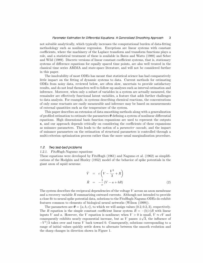
The parameters are θ = {a, b, c}, to which we will assign values (0.2, 0.2, 3), respectively.The R equation is the simple constant coefficient linear system R = −(b/c)R with linearinputs V and a. However, the V equation is nonlinear; when V > 0 is small, V ≈ cV andconsequently exhibits nearly exponential increase, but as V passes ±√3, the influence of−V 3/3 takes over and turns V back toward 0. Consequently, solutions corresponding to arange of initial values quickly settle down to alternate between the smooth evolution andthe sharp changes in direction shown in Figure 1.

0 5 10 15 20−2

0

2

4

V

0 5 10 15 20−1

0

1

2

R

Fig. 1. The limiting behavior of voltage V and recovery R variables de�ned by the FitzHugh-Nagumoequations (2) with parameter values a = 0.2, b = 0.2 and c = 3.0 and initial conditions (V0, R0) =(−1, 1). The horizontal axis is time in milliseconds.

−1−0.5

00.5

11.5 −1

0

1

0

500

1000

1500

ba

Fig. 2. A response surface for solutions of the FitzHugh-Nagumo equations (2) as parameters a andb are varied. Surface values give the integrated squared difference between solutions at parametersa = 0.2, b = 0.2 with solutions at the values of a and b given on the x and y axes, respectively; c = 3and initial conditions V (0) = −1, R(0) = 1 are held constant.


A concern in dynamic systems modeling is the possibly complex nature of the fit sur-face. The existence of many local minima has been commented on in Esposito and Floudas(2000); and a number of computationally demanding algorithms, such as simulated an-nealing, have been proposed to overcome this problem. For example, Jaeger et al. (2004)reported using weeks of computation to compute a point estimate. Figure 2 displays theintegrated squared difference between the paths in Figure 1 and those resulting from varyingonly the parameters a and b. The features of this surface include “ripples” due to changesin the shape and period of the limit cycle and breaks due to bifurcations, or sharp changesin behavior.

1.2.2. Tank reactor equationsThe chemical engineering concept of a continuously stirred tank reactor (CSTR) consistsof a tank surrounded by a cooling jacket containing an impeller which stirs its contents. Afluid containing a reagent with concentration Cin enters the tank at a flow rate Fin andtemperature Tin. A reaction produces a product that leaves the tank with concentration Cand temperature T . A coolant in the cooling jacket has temperature Tco and flow rate Fco.

The differential equations used to model a CSTR, simplified by setting the volume ofthe tank to one, are

C = −βCC(T, Fin)C + FinCin

T = −βTT (Fco, Fin)T + βTC(T, Fin)C + FinTin + α(Fco)Tco. (3)

The input variables play two roles in the right sides of these equations: through addedterms such as FinCin and FinTin, and via the weight functions βCC , βTC , βTT and α thatmultiply the output variables and Tco, respectively. These time-varying multipliers dependon four system parameters as follows:

βCC(T, Fin) = κ exp[−104τ(1/T − 1/Tref )] + Fin

βTT (Fco, Fin) = α(Fco) + Fin

βTC(T, Fin) = 130βCC(T, Fin)α(Fco) = aF b+1

co /(Fco + aF bco/2), (4)

where Tref is a fixed reference temperature within the range of the observed temperatures,and in this case was 350 deg K. These functions are defined by two pairs of parameters:(τ, κ) defining coefficient βCC and (a, b) defining coefficient α. The factor 104 in βCC rescalesτ so that all four parameters are within [0.4, 1.8]. These parameters are gathered in thevector θ in (1), and determine the rate of the chemical reactions involved, or the reactionkinetics.

The plant engineer needs to understand the dynamics of the two output variables C andT as determined by the five inputs Cin, Fin, Tin, Tco and Fco. A typical experiment designedto reveal these dynamics is illustrated in Figure 3, where we see each input variable steppedup from a baseline level, stepped down, and then returned to baseline. Two baseline levelsare presented for the most critical input, the coolant temperature Tco.

The behaviors of output variables C and T under the two experimental regimes, givenvalues 0.833, 0.461, 1.678 and 0.5 for parameters τ, κ, a and b, respectively, are shown inFigure 4. When the reactor runs in the cool mode, where the baseline coolant temperatureis 335 degrees Kelvin, the two outputs respond smoothly to the step changes in all inputs.

0 10 20 30 40 50 600.5

1

1.5

F(t)

0 10 20 30 40 50 60

1.82

2.2

C0(t)

0 10 20 30 40 50 60300

350

T0(t)

0 10 20 30 40 50 60

340

360

Tco

(t)

0 10 20 30 40 50 60101520

Fc(t)

Fig. 3. The �ve inputs to the chemical reactor modeled by the equations (3) and (4): �ow rate F (t),input concentration C0(t), input temperature T0(t), coolant temperature Tco(t) and coolant �ow F0(t).Coolant temperature Tco(t) was set at two baseline levels, cool and hot.

0 10 20 30 40 50 600

0.5

1

1.5

2

C(t)

(%)

Cool Hot

0 10 20 30 40 50 60

340

360

380

400

420

t (min)

T(t)

(deg

K)

Fig. 4. The two outputs, for each of baseline coolant temperatures Tco of 335 and 365 deg. K, fromthe chemical reactor modeled by the two equations (3): concentration C(t) and temperature T (t).The input functions are shown in Figure 3. Times at which an input variable Tco(t) was stepped downand then up are shown as vertical dotted lines.


However, an increase in baseline coolant temperature by 30 degrees Kelvin generates oscil-lations that come close to instability when the coolant temperature decreases, somethingthat is undesirable in an actual industrial process. These perturbations are due to the dou-ble impact of a decrease in output temperature, which increases the size of both βCC andβTC . Increasing βTC raises the forcing term in the T equation, thus increasing tempera-ture. Increasing βCC makes concentration more responsive to changes in temperature, butdecreases the size of the response. This push–pull process has a resonant frequency thatdepends on the kinetic constants, and when the ambient operating temperature reaches acertain level, the resonance appears. For coolant temperatures either above or below thiscritical zone, the oscillations disappear.

The CSTR equations present two challenges that are not an issue for the Fitz-HughNagumo equations. The step changes in inputs induce corresponding discontinuities inthe output derivatives that complicate the estimation of solutions by numerical methods.Moreover, the engineer must estimate the reaction kinetics parameters in order to estimatethe cooling temperature range to avoid, but a key question is whether all four parametersare actually estimable given a particular data configuration. Step changes in inputs andnear over-parameterization are common problems in dynamic systems modeling.

1.3. Review of current ODE parameter estimation strategiesProcedures for estimating the parameters defining an ODE from noisy data tend to fallinto three broad classes: linearization, discretization methods for initial value problemsand basis function expansion or collocation methods for boundary and distributed dataproblems. Linearization involves replacing nonlinear structures by first order Taylor seriesexpansions, and tends only to be useful over short time intervals combined with rather mildnonlinearities, and will not be considered further. There is a large literature on numericalmethods for solving constrained optimization problems, under which parameter estimationusually falls; see Biegler and Grossman (2004) for an excellent overview.

1.3.1. Data fitting by numerical approximation of an initial value problemThe numerical methods most often used to approximate solutions of ODEs over a range[t0, t1] use fixed initial values x0 = x(t0) and adaptive discretization techniques (Biegleret al. (1986)). The data fitting process, often referred to by textbooks as the nonlinear leastsquares or NLS method, works as follows. A numerical method such as the Runge-Kuttaalgorithm is used to approximate the solution given a trial set of parameter values and initialconditions, a procedure referred to by engineers as simulation. The fit value is input intoan optimization algorithm that updates parameter estimates. If the initial conditions x(0)are unavailable, they must be appended to the parameters θ as quantities with respect towhich the fit is optimized. The optimization process can proceed without using gradients,or these may also be approximated by solving the sensitivity differential equations

d

dt

(dxdθ

)=

∂f∂θ

+∂f∂x

dxdθ

, withdxdθ

∣∣∣∣t=0

= 0. (5)

In the event that x(0) = x0 must also be estimated, the corresponding sensitivity equationsare

d

dt

(dxdx0

)=

∂f∂x

dxdx0

, withdxdx0

∣∣∣∣t=0

= I. (6)

Systems for which solutions beginning at varying initial values tend to converge to a commontrajectory are called stiff, and require special methods that make use of the Jacobian ∂f/∂x.

The NLS procedure has many problems. It is computationally intensive since a numer-ical approximation to a possibly complex process is required for each update of parametersand initial conditions. The inaccuracy of the numerical approximation can be a problem,especially for stiff systems or for discontinuous inputs such as step functions or functionsconcentrating their masses at discrete points. The size of the parameter set may be in-creased by the set of initial conditions needed to solve the system, and the data may notprovide much information for estimating them. NLS also only produces point estimates ofparameters, and where interval estimation is needed, a great deal more computation canbe required. As a consequence of all this, Marlin (2000) warns process control engineers toexpect an error level of the order of 25% in parameter estimates.

A Bayesian approach which may escape minor ripples in the optimization surface isoutlined in Gelman et al. (1996). This model uses a likelihood centered on the numericalsolution to the differential equation x(tj |θ), such as yj ∼ N [x(tj |θ), σ2]. Since x(tj |θ) hasno closed form solution, the posterior density for θ | y has no closed form and inferencemust be based on simulation from a Metropolis-Hastings algorithm or other sampler. Ateach iteration of the sampler θ is proposed and the numerical approximation x(tj |θ) is usedto compute the likelihood. Parallels between this approach and NLS mean that they sharemany of the same optimization problems. To fix this, the Bayesian model often requiresstrong finitely bounded priors. Extensions to this method are outlined in Campbell (2007).

1.3.2. Collocation methods or basis function expansionsOur own approach belongs in the family of collocation methods that express the approxi-mation xi of xi in terms of a basis function expansion

xi(t) =Ki∑

k

cikφik(t) = c′iφi(t), (7)

where the number Ki of basis functions in vector φi is chosen so as to ensure enoughflexibility to capture the variation in the approximated function xi and its derivatives.Typically, this will require substantially more flexibility than is required to fit the data, sincexi and dx/dt must also satisfy the differential equation to an extent considered acceptable.Although the original collocation methods used polynomial bases, spline basis systems arenow preferred because they allow control over the smoothness of the solution at specificvalues of t, including discontinuities in dx/dt or higher order derivatives associated withstep and point changes in the inputs u. Using a spline basis to approximate an initial valueproblem is equivalent to the use of an implicit Runge-Kutta method for stepping pointslocated at the knots defining the basis (Deuflhard and Bornemann (2000)). For solvingboundary value problems, collocation tries to satisfy (1) at a discrete set of points; resultingin a large sparse system of nonlinear equations which must then be solved numerically.

Collocation with spline bases was applied to dynamic data fitting problems by Varah(1982), who suggested a two-stage procedure in which each xi is first estimated by datasmoothing methods without considering (1), followed by the minimization of a least squaresmeasure of the fit of dx/dt to f(x,u, t|θ) with respect to θ. The method is attractive whenf is nearly linear in θ, but nonlinear in x. Varah’s approach worked well for the simpleequations that were considered, but considerable care was required in the smoothing step


to ensure a satisfactory estimate of x, and the technique also required that all variables inthe system be measured.

Ramsay and Silverman (2005) and Poyton et al. (2006) took Varah’s method furtherby iterating the two steps, and replacing the previous iteration’s roughness penalty by apenalty on ‖dx/dt − f(x,u, t|θ)‖ using the last minimizing value of θ. They found thatthis process, iterated principal differential analysis (iPDA), converged quickly to estimatesof both x and θ that had substantially improved bias and precision. However, iPDA is ajoint estimation procedure in the sense that it optimizes a single roughness-penalized fittingcriterion with respect to both c and θ, an aspect that will be discussed further in the nextsection.

A number of procedures have attempted to solve the parameter estimation problem atthe same time as computing a numerical solution to (1). Tjoa and Biegler (1991) proposesto combine a numerical solution of the collocation equations with an optimization overparameters to obtain a single constrained optimization problem, see also Arora and Biegler(2004). Similar ideas can be found in Bock (1983), where the multiple shooting method isproposed that breaks the time domain into a series of smaller intervals, over each of which(1) is solved.

1.4. Overview of the paperOur approach to fitting differential equation models is developed in Section 2, where wedevelop the concepts of estimating functions and a generalization of profiled estimation.Section 3 tests the method on simulated data for the FitzHugh-Nagumo and CSTR equa-tions, and Section 4 estimates differential equation models for data drawn from chemicalengineering and medicine. Generalizations of the method are discussed in Section 5.

2. Generalized pro�ling estimation procedure

We first give an overview of our estimation strategy, and then provide further details below.As we noted above, our method is a variant of the collocation method, and as such, repre-sents each variable in terms of a basis function expansion (7). Let c indicate the compositevector of length K =

∑i∈I Ki that results from concatenating the ci’s. Let Φi be the

Ni by Ki matrix of values φk(tij), and let Φ be the N =∑

i∈I Ni by K super–matrixconstructed by placing the matrices Φi along the diagonals and zeros elsewhere. Accordingto this notation, we have the composite basis expansion x = Φc.

2.1. Overview of the estimation procedureDefining x as a set of basis function expansions implies that there are two classes of param-eters to estimate: the parameters θ defining the equation, such as the four reaction kineticsparameters in the CSTR equations; and the coefficients in ci defining each basis functionexpansion. The equation parameters are structural in the sense of being of primary interest,as are the error distribution parameters in σi, i ∈ I. But the coefficients ci are consideredas nuisance parameters that are essential for fitting the data, but usually not of direct con-cern. The sizes of these vectors are apt to vary with the length of the observation interval,density of observation, and other aspects of the structure of the data; and the number ofthese nuisance parameters can be orders of magnitude larger than the number of struc-

tural parameters, with a ratio of about 200 applying in the CSTR and FitzHugh-Nagumoproblems.

In our profiling procedure, the nuisance parameter estimates are defined to be implicitfunctions ci(θ, σ; λ) of the structural parameters, in the sense that each time θ and σare changed, an inner fitting criterion J(c|θ,σ, λ) is re-optimized with respect to c alone.The estimating function ci(θ,σ; λ) is regularized by incorporating a penalty term in J thatcontrols the size of the extent that x = c′φ fails to satisfy the differential equation exactly,in a manner specified below. The amount of regularization is controlled by smoothingparameters in vector λ. This process of eliminating the direct impact of nuisance parameterson the fit of the model to the data resembles the common practice of eliminating randomeffect parameters in mixed effect models by marginalizing over c with respect a prior density.

A data fitting criterion H(θ,σ|λ) is then optimized with respect to the structural pa-rameters alone. The dependency of H on (θ,σ) is two-fold: directly, and implicitly throughthe involvement of ci(θ, σ;λ) in defining the fit xi. Because ci(θ, σ; λ) is already regular-ized, criterion H does not require further regularization, and is a straightforward measureof fit such as error sum of squares, log likelihood or some other measure that is appropriategiven the distribution of the errors eij .

For the examples in this paper, λ has been adjusted manually using some numericaland visual heuristics. However, we also envisage that λ may be estimated automaticallythrough the use of a measure F (λ) of model complexity or mean squared error, such as thegeneralized cross-validation or GCV criterion often used in least squares spline smoothing.In this event, the vector λ defines a third level of parameters, and leads us to define a pa-rameter cascade in which structural parameter estimates are in turn defined to be functionsθ(λ) and σ(λ) of regularization or complexity parameters, and nuisance parameters nowalso become functions of λ via their dependency on structural parameters. We have appliedthis notion to semi-parametric regression in Cao and Ramsay (2006) where the estimationprocedure is a multi-criterion optimization problem, and we can refer to J,H and F asinner, middle and outer criteria, respectively. Keilegom and Carroll (2006) use a similarapproach, also in semi-parametric regression.

We motivate this approach as follows. Fixing complexity parameters λ for the purposesof discussion, we appreciate here, as in random effects modeling and nonparametric regres-sion, that it would be unwise to employ joint estimation using a fixed data-fitting criterionH with respect to all of θ, σ and c since the overwhelmingly larger number of nuisanceparameters would tend to lead to over-fitting the data and consequently unacceptable biasand sampling variance in θ and σ. By assessing smoothness of the fit x to the data interms of departure from satisfying (1), we are, in effect, bringing additional “data” into thefitting process in the form of the roughness penalty in much the same way that a Bayesianbrings prior information to parameter estimation in the form of the logarithm of a priordensity. However, the Bayesian strategy suffers from the problem that the integration inthe marginalization process is seldom available analytically, thus leading to computationallyintensive MCMC technology. We show here that our parameter cascade approach leads toanalytic derivatives required for efficient optimization, and also for linear approximation tointerval estimates.

2.2. Data �tting criterionLet ei indicate the vector of errors associated with observed variable i ∈ I, and let gi(ei|σi)indicate the joint density of these errors conditional on a parameter vector σi. In practice


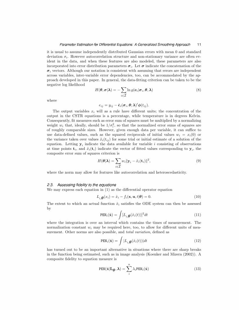
it is usual to assume independently distributed Gaussian errors with mean 0 and standarddeviation σi. However autocorrelation structure and non-stationary variance are often ev-ident in the data, and when these features are also modeled, these parameters are alsoincorporated into error distribution parameters σi. Let σ indicate the concatenation of theσi vectors. Although our notation is consistent with assuming that errors are independentacross variables, inter-variable error dependencies, too, can be accommodated by the ap-proach developed in this paper. In general, the data-fitting criterion can be taken to be thenegative log likelihood

H(θ, σ|λ) = −∑

i∈Iln g(ei|σi, θ,λ) (8)

whereeij = yij − ci(σi, θ; λ)′φ(tij).

The output variables xi will as a rule have different units; the concentration of theoutput in the CSTR equations is a percentage, while temperature is in degrees Kelvin.Consequently, fit measures such as error sum of squares must be multiplied by a normalizingweight wi that, ideally, should be 1/σ2

i , so that the normalized error sums of squares areof roughly comparable sizes. However, given enough data per variable, it can suffice touse data-defined values, such as the squared reciprocals of initial values wi = xi(0) orthe variance taken over values xi(tij) for some trial or initial estimate of a solution of theequation. Letting yi indicate the data available for variable i consisting of observationsat time points ti, and xi(ti) indicate the vector of fitted values corresponding to yi, thecomposite error sum of squares criterion is

H(θ|λ) =∑

i∈Iwi‖yi − xi(ti)‖2, (9)

where the norm may allow for features like autocorrelation and heteroscedasticity.

2.3. Assessing �delity to the equationsWe may express each equation in (1) as the differential operator equation

Li,θ(xi) = xi − fi(x,u, t|θ) = 0. (10)

The extent to which an actual function xi satisfies the ODE system can then be assessedby

PENi(x) =∫

[Li,θ(xi(t))]2dt (11)

where the integration is over an interval which contains the times of measurement. Thenormalization constant wi may be required here, too, to allow for different units of mea-surement. Other norms are also possible, and total variation, defined as

PENi(x) =∫|Li,θ(xi(t))|dt (12)

has turned out to be an important alternative in situations where there are sharp breaksin the function being estimated, such as in image analysis (Koenker and Mizera (2002)). Acomposite fidelity to equation measure is

PEN(x|Lθ,λ) =n∑

i

λiPENi(x) (13)

where Lθ denotes the vector containing the d differential operators Li,θ. Note that in this

case the summation will be over all d variables in the equation. The multipliers λi ≥ 0permit us to weight fidelities differently, and also control the relative emphasis on fittingthe data and solving the equation for each variable.

2.4. Estimating c(θ; λ)Finally, the data-fitting and equation-fidelity criteria are combined into the penalized loglikelihood criterion

J(c|θ, σ,λ) = −∑

i∈Iln g(ei|σi, θ, λ) + PEN(x|λ), (14)

or the least squares criterion

J(c|θ, σ, λ) =∑

i∈Iwi‖yi − xi(ti)‖2 + PENi(x|λ). (15)

In general the minimization of J will require numerical optimization, but in the least squarescase and linear ODEs, it is possible to express c(θ; λ) analytically (Ramsay and Silverman(2005)).

2.5. Optimizing with respect to θIn this and the remainder of the section, we simplify the notation considerably by droppingthe dependency of criterion H on σ and λ; and regarding the latter as a fixed parameter.These results can easily be extended to get the results for the joint estimation of systemparameters θ and error distribution parameters σ where required. It is assumed that H istwice continuously differentiable with respect to both θ and c, and that the second partialderivative or Hessian matrices ∂2H/∂θ2 and ∂2H/∂c2 are positive definite over a nonemptyneighborhood N of y in data space.

The gradient or total derivative with respect to θ is

dH

dθ=

∂H

∂θ+

∂H

∂cdcdθ

. (16)

Since c(θ) is not available explicitly, we apply the Implicit Function Theorem to obtain

dcdθ

= −(

∂2J

∂c2

)−1∂2J

∂c∂θ. and

dH

dθ=

∂H

∂θ− ∂H

∂c

(∂2J

∂c2

)−1∂2J

∂c∂θ. (17)

The matrices used in these equations and those below have complex expressions in termsof the basis functions in Φ and the functions f on the right side of the differential equation.Appendix A provides explicit expressions for them for the case of least squares estimation.

2.6. Approximating the sampling variation of θ and cLet Σ be the variance–covariance matrix for y. Making explicit the dependency of H onthe data y by using the notation H(θ|y), the estimate θ(y) of θ is the solution of thestationary equation ∂H(θ, |y)/∂θ = 0. Here and below, all partial derivatives as well as


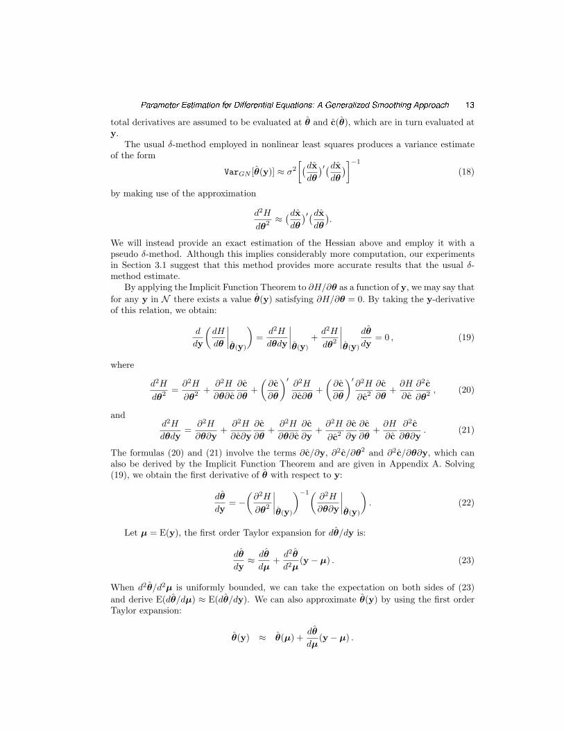
total derivatives are assumed to be evaluated at θ and c(θ), which are in turn evaluated aty.

The usual δ-method employed in nonlinear least squares produces a variance estimateof the form

VarGN [θ(y)] ≈ σ2

[(dxdθ

)′(dxdθ

)]−1

(18)

by making use of the approximation

d2H

dθ2 ≈ (dxdθ

)′(dxdθ

).

We will instead provide an exact estimation of the Hessian above and employ it with apseudo δ-method. Although this implies considerably more computation, our experimentsin Section 3.1 suggest that this method provides more accurate results that the usual δ-method estimate.

By applying the Implicit Function Theorem to ∂H/∂θ as a function of y, we may say thatfor any y in N there exists a value θ(y) satisfying ∂H/∂θ = 0. By taking the y-derivativeof this relation, we obtain:

d

dy

(dH

dθ

∣∣∣∣ˆθ(y)

)=

d2H

dθdy

∣∣∣∣ˆθ(y)

+d2H

dθ2

∣∣∣∣ˆθ(y)

dθ

dy= 0 , (19)

where

d2H

dθ2 =∂2H

∂θ2 +∂2H

∂θ∂c∂c∂θ

+(

∂c∂θ

)′∂2H

∂c∂θ+

(∂c∂θ

)′∂2H

∂c2

∂c∂θ

+∂H

∂c∂2c∂θ2 , (20)

andd2H

dθdy=

∂2H

∂θ∂y+

∂2H

∂c∂y∂c∂θ

+∂2H

∂θ∂c∂c∂y

+∂2H

∂c2

∂c∂y

∂c∂θ

+∂H

∂c∂2c

∂θ∂y. (21)

The formulas (20) and (21) involve the terms ∂c/∂y, ∂2c/∂θ2 and ∂2c/∂θ∂y, which canalso be derived by the Implicit Function Theorem and are given in Appendix A. Solving(19), we obtain the first derivative of θ with respect to y:

dθ

dy= −

(∂2H

∂θ2

∣∣∣∣ˆθ(y)

)−1(∂2H

∂θ∂y

∣∣∣∣ˆθ(y)

). (22)

Let µ = E(y), the first order Taylor expansion for dθ/dy is:

dθ

dy≈ dθ

dµ+

d2θ

d2µ(y− µ) . (23)

When d2θ/d2µ is uniformly bounded, we can take the expectation on both sides of (23)and derive E(dθ/dµ) ≈ E(dθ/dy). We can also approximate θ(y) by using the first orderTaylor expansion:

θ(y) ≈ θ(µ) +dθ

dµ(y− µ) .

Taking variance on both sides of (24), we derive

Var[θ(y)] ≈[

dθ

dµ

]Σ

[dθ

dµ

]′≈

[dθ

dy

]Σ

[dθ

dy

]′, since E

(dθ

dµ

)≈ E

(dθ

dy

). (24)

Similarly, the sampling variance of c[θ(y)] is estimated by

Var[c(θ(y))] =( dcdy

)Σ( dcdy

)′ , wheredcdy

=dc

dθ

dθ

dy+

∂c∂y

. (25)

2.7. Numerical integration in the inner optimizationThe integrals in PENi will normally require approximation by the linear functional

PENi(x) ≈Q∑q

vq[Li(xi(tq))]2 (26)

where Q, the evaluation points tq, and the weights vq are chosen so as to yield a reasonableapproximation to the integrals involved.

Let ξ` indicate a knot location or a breakpoint, and recall that there will be multipleknots at such a location in order to deal with step function inputs that will imply discontin-uous derivatives. We divide each interval [ξ`, ξ`+1] into four equal-sized intervals, and usingSimpson’s rule weights [1, 4, 2, 4, 1](ξ`+1 − ξ`)/5. The total set of these quadrature pointsand weights along with basis function values may be saved at the beginning of the compu-tation so as to save time. If a B-spline basis is used, improvements in speed of computationmay be achieved by using sparse matrix methods.

Efficiency in the inner optimization is essential since this will be invoked far more oftenthan the outer optimization. In the case of least squares fitting, the minimization of (14)can be expressed as a large nonlinear least squares approximation problem by observingthat we can express the numerical quadrature approximation to

∑i λiPENi(x) as

∑

i

∑q

[(λivq)1/2Li(xi(tq))]2.

These squared residuals can then be appended to those in H, and Gauss-Newton minimiza-tion can then be used.

2.8. Choosing the amount of smoothingWe now consider two rationales for choosing λ, corresponding to the need for robustness withrespect to poor initial parameter values or model mis-specification, respectively. Although λwas chosen manually for our examples, this choice can be automated under either paradigm,and we suggest some ways of doing so.

2.8.1. Robustness with respect to initial parameter valuesFigure 2 shows the severe non-convexity of least-squares fitting criteria for θ when using anexact solution of the FitzHugh-Nagumo ODE, implying a small neighborhood of the opti-mal parameter values from which convergence is assured using the Gauss-Newton method.


However, Figure 5, displaying the much more regular surface corresponding to λ = 105,suggests a much wider region of convergence; and our experience for other problems con-firms this robustness with respect to poor initialization of parameters for smaller λ values.Because the criterion H(θ, σ|λ) is increasing in each λi, it underestimates the responsesurface for exact solutions to the differential equation. Moreover, results in Appendix Aimply that ‖dc/dθ‖ increases in λ, implying that relaxing the differential equation modelregularizes the search for θ.

However, as λ becomes smaller, the estimates obtained for θ become both more biasedand more variable. Theorem 2.2, on the other hand, demonstrates that, ignoring errordue to (7), parameter estimates must approximate those that would have been obtainedfrom a straightforward maximum-likelihood fit as λ increases. This suggests the followingalgorithm:

(a) Choose initial value λ0 so that H(θ|σ,λ0) dominates PEN(x|Lθ, λ0).(b) Increase λi iteratively, and estimate θi, initializing the Gauss-Newton algorithm with

parameter estimates θi−1. We typically choose λi = 10i−k where k represents astarting value.

(c) Stop when λ0 becomes so large that the collocation approximation (7) starts to distortthe estimate of x.

In order to assess when λ has become too large:

(a) Calculate solutions x(t) to (1) with the current estimate of θ and x0.(b) Smooth x(t), the solution at the observation times, using the model-based criterion

(14) to get an estimate x∗.(c) Stop when ‖x− x∗‖ begins to increase after attaining a minimum.

We have observed that there is usually a large range of λ values that provide stable andaccurate estimates for θ.

For the simulated examples in Section 3 and for the Nylon production data, we chose λlarge enough to guarantee that we could reproduce solutions to (1) to a visually high degreeof accuracy without suffering distortion from the use of a basis expansion.

2.8.2. Robustness with respect to model mis-specification

For the Lupus data in Section 4.2, the ODE model provides only a partially adequate fitto the data, and consequently the optimal value of λ is not infinite. In such situations,a practical method of choosing λ is by visual inspection of the fit to the observed data,aided by examining the corresponding ODE solution at the estimated parameters. Initialconditions x(0) may be taken from the smooth x(0), or may be separately optimized.

When the objective is filtering the data, a GCV-type approach may be appropriate.The estimation of x given λ is in general a nonlinear problem, so standard cross-validationmeasures are not available. Instead, the following GCV-like criterion has been adapted fromWahba (1990):

F (λ) =∑I ‖yi − xi(ti)‖2[∑

I(Ni −

∑j

dxi(tij)dyij

)]2 , (27)

−0.5

0

0.5

1

−0.5

0

0.5

10

1000

2000

3000

ba

Fig. 5. The squared discrepancy between exact solutions to the FitzHugh-Nagumo equations and amodel based smooth that minimizes (14) with λ = 105. Values of the surface are calculated usingthe same data as in Figure 2.

where the derivatives in the denominator are exactly the diagonal elements of the smoothingmatrix in a linear smoothing problem. For the profiling procedure outlined above we have

dxi(tij)dyij

=∂xi(tij)

∂cdc

dyij

where dxi(tij)/dc is simply the value of the basis expansion (7) at tij and dc/dy hasbeen calculated in (24). Note that this explicitly takes the dependence of y on θ intoaccount. This construction is offered as speculation; it is well known that the first orderapproximation used in F (λ) can be biased (Friedman and Silverman (1989)). Furthermore,F (λ) is only indirectly related to θ, and our experience suggests that, for mis-specifiedmodels, estimators based on cross-validation tend select λ at values that produce goodestimates of x, but which are smaller than optimal for estimating θ.

2.9. Parameter estimate behavior as λ →∞In this section, we consider the behavior of our parameter estimate as λ becomes large.This analysis takes an idealized form in the sense that we assume that this optimizationmay be done globally and that the function being estimated can be expressed exactly andwithout the approximation error that would come from a basis expansion. We show thatas λ becomes large, the estimates defined through our profiling procedure converge to theestimates that we would obtain if we estimated θ by minimizing negative log likelihood overboth θ and the initial conditions x0. In other words, we treat x0 as nuisance parametersand estimate θ by profiling. When f is Lipschitz continuous in x and continuous in θ, the


likelihood is continuous in θ and the usual consistency theorems (e.g. Cox and Hinkley(1974)) hold and in particular, the estimate θ is asymptotically unbiassed.

For the purposes of this section, we will make a few simplifying conventions. Firstly, wewill take:

l(x) = −∑

i∈Iln g(ei|σi, θ, λ).

Secondly, we will represent

PEN(x|θ) =n∑

i=1

ciwi

∫(xi(t)− fi(x,u, t|θ))2 dt

where the ci are taken to be constants and the λi used in the definition (13) are given byλci for some λ.

We will also assume that solutions to the data fitting problem exist and are well defined,and that there are objects x that satisfy PEN(x|θ) = 0. Such objects are guaranteed to existlocally whenever f is locally Lipschitz continuous. That is, there is a time interval [t0, t0 +h]on which x exists. On this interval x is uniquely determined by x(t0); see Deuflhard andBornemann (2000). Existence on the interval of the experiment is more difficult to show ingeneral.

Finally, we will need to make some assumptions about the spline smooths minimizing

l(x) + λPEN(x|θ).

Specifically, we will assume that the minimizers of these are well-defined and boundeduniformly over λ. Guarantees on boundedness may be given whenever x · f(x,u, t|θ) < 0for ‖x‖ greater than some K (see Hooker (2007)). This condition is also sufficient forthe global uniqueness of solutions to (1). It is true for reasonable parameter values in allsystems presented in this paper. More general characteristics of functions f for which theseproperties hold is a matter of continued research.

Solutions of interest lie in the Hilbert space H = (W 1)n; the direct sum of n copies ofW 1 where W 1 is the Sobolev space of functions on the the time-observation interval [t1, t2]whose first derivatives are square integrable. The analysis will examine both inner andouter optimization problems as λ →∞. For the inner optimization, we can show

Theorem 2.1. Let λk →∞ and assume that

xk = argminx∈(W 1)n

l(x) + λkPEN(x|θ)

is well defined and uniformly bounded over λ. Then xk converges to x∗ with PEN(x∗|θ) = 0.

Further, when PEN(x|θ) is given by (13), x∗ is the solution of the differential equations(1) that is obtained by minimizing squared error over the choice of initial conditions. Theproof of this, and of the theorem below, is given in Hooker (2007).

Turning to the estimation of θ, we obtain the following:

Theorem 2.2. Let X ⊂ (W 1)n and Θ ⊂ Rp be bounded. Assume that for λ > K,

xθ,λ = argminx∈X

l(x) + λPEN(x|θ)

is well defined for each θ. Define x∗θ to be such that

l(x∗θ) = minx:P (x|θ)=0

l(x)

and letθ(λ) = argmin

θ∈Θ

l(xθ,λ) and θ∗ = argmin

θ∈Θ

l(x∗θ)

also be well defined. Thenlim

λ→∞θ(λ) = θ∗.

The conditions listed in this theorem are natural, in the sense that we merely requirethat the smoothing, parameter estimation and NLS optimization problems to have uniquesolutions. However, verifying that this is the case, even for the NLS problem, many not bestraightforward for any given f. We note a substantial literature on system identifiability:for example Denis-Vidal et al. (2003). We conjecture that it will hold for any f such thatthe parameter estimation problem is well defined for exact solutions to (1).

Taken together, these theorems state that as λ is increased, the solutions obtained fromthis scheme tend to those that would be obtained by estimating the parameters directlywhile profiling out the initial conditions. In particular, the path of parameter values as λchanges is continuous, motivating a successive approximation scheme. This analysis alsohighlights the distinction between these methods and traditional smoothing; our penaltiesare highly informative and it is, in fact, the data which plays the minor role in finding asolution.

3. Simulated data examples

3.1. Fitting the FitzHugh-Nagumo equationsWe set up simulated data for V alone by adding Gaussian error with standard deviation 0.5to the solution for parameters {a, b, c} = {0.2, 0.2, 3} and initial conditions {V, R} = {−1, 1}at times 0.0, 0.05, . . . , 20.0. Collocation fit x was a third order B-spline with knots at eachdata point.

Figure 6 gives quartiles of the parameter estimates for 60 simulations as λ is varied from10−2 to 105. There is large bias for small values of λ, where smoothing is emphasized andθ has little impact on c; but, as λ increases, parameter estimates become nearly unbiased.Table 3.1 provides bias and variance estimates from 500 simulations at λ = 104, along withour estimate (24) and the Gauss-Newton standard error (18). We obtain good coverageproperties for our estimates of variance while the Gauss-Newton estimates are somewhatless accurate. We note, however, that computing (24) increased computational effort by afactor of about 10 for this simulation. As a practical matter, using (18) may be consideredsufficient if (24) becomes too costly.

3.2. Fitting the tank reactor equationsData for concentration C and temperature T were simulated by adding zero mean Gaussiannoise with standard deviations 0.0223 and 0.79, respectively to the values for the cool modeexperimental condition shown in Figure (4). These error levels were about 20% of the vari-ation of the respective outputs over the experimental conditions, an error level considered


−2 −1 0 1 2 3 4−0.5

0

0.5

1

1.5

2

2.5

3

3.5

log10

lambda

para

met

er e

stim

ates

abc

Fig. 6. 25%, 50% and 75% quantiles of parameter estimates for the FitzHugh-Nagumo Equations asλ is varied. Horizontal lines represent the true parameter values.

Table 1. Summary statistics for parameter estimatesfor 500 simulated samples of data generated from theFitzHugh-Nagumo equations.

a b c

True value 0.2000 0.2000 3.0000Mean value 0.2005 0.1984 2.9949Bias Std. Err. 0.0007 0.0029 0.0012

Actual Std. Dev. 0.0149 0.0643 0.0264Estimate (24) Std. Dev. 0.0143 0.0684 0.0278Estimate (18) Std. Dev. 0.0167 0.0595 0.0334

Table 2. Summary statistics for parameter estimates for 1000 simulated samples.Results are for measurements on both concentration and temperature, and also fortemperature measurements only. The estimate of the standard deviation of parametervalues is by the delta method usual in nonlinear least squares analyses.

C and T data Only T data

κ τ a κ τ a

True value 0.4610 0.8330 1.6780 0.4610 0.8330 1.6780Mean value 0.4610 0.8349 1.6745 0.4613 0.8328 1.6795Bias Std. Err. 0.0002 0.0004 0.0012 0.0005 0.0005 0.0024

Actual Std. Dev. 0.0034 0.0057 0.0188 0.0084 0.0085 0.0377Estimate (18) Std. Dev. 0.0035 0.0056 0.0190 0.0088 0.0090 0.0386

typical for many chemical engineering processes. We estimated only the parameters κ, τand a, keeping b fixed at 0.5 because we had determined that the accurate estimation ofall four parameters is impossible within the data design described above. Since the dataare generated here from functions satisfying the differential equation system, we can expectthe fit to improve with larger and larger values for smoothing parameters λC and λT . Re-sults are reported here for 100 and 10, respectively, which are sufficiently large that furtherincreases were found to yield negligible improvement in parameter estimates.

We found, in applying the NLS method described in Section 1.3.1, that the approxi-mation to T (t) at the times of input step changes using the Runge-Kutta algorithm wereinaccurate and unstable with respect to small changes in parameters. As a consequence,the estimation of the gradient of fit (9) by differencing was so unstable that gradient-freeoptimization was impossible. When we estimated the gradient by solving the sensitivityequations (5) and (6), we could only achieve optimization when starting values for param-eters and initial values were much closer to the optimal values than could be realized inpractice. By contrast, our approach was able to converge reliably from random startingvalues far removed from the optimal estimates.

Table 3.2 displays bias and sampling precision results for parameter estimates by ourparameter cascade method for 1000 simulated samples for each of two measurement regimes:both variables measured, and only temperature measured. The first two lines of the tablecompare the true parameter values with the mean estimates, and the last two lines comparethe biases of the estimates with the standard errors of the mean estimates. We see thatthe estimation biases can be considered negligible for both measurement situations. Thethird and fourth lines compare the actual standard deviations of the parameter estimateswith the values estimated with the Gauss-Newton method in (18), and the two valuesseem sufficiently close for all three parameters to permit us to trust the Gauss-Newtonestimates in this case. As one might expect, the main impact of having only temperaturemeasurements is to increase the sampling error in the parameter estimates.

When the equations were solved using the parameters estimated from measurements onboth variables, the maximum absolute discrepancy between the fitted and true curves was0.11% and 0.03%, respectively, and when these parameter estimates were used for the hotmode of operation, the the discrepancies became 1.72% and 0.05%, respectively. Finally,when the parameters were estimated from only the temperature data, the concentrationand temperature discrepancies in cool mode became 0.10% and 0.04%, respectively, so thatusing only the quickly and cheaply attainable temperature measurements is sufficient foridentifying this system in either mode of operation.


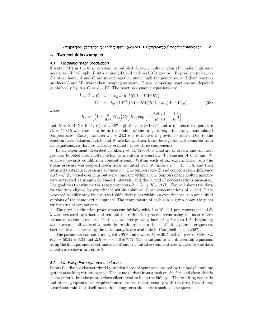
4. Two real data examples

4.1. Modeling nylon productionIf water (W ) in the form of steam is bubbled through molten nylon (L) under high tem-peratures, W will split L into amine (A) and carboxyl (C) groups. To produce nylon, onthe other hand, A and C are mixed together under high temperatures, and their reactionproduces L and W , water then escaping as steam. These competing reactions are depictedsymbolically by A + C L + W . The reaction dynamic equations are

−L = A = C = −kp ∗ 10−3(CA− LW/Ka)

W = kp ∗ 10−3(CA− LW/Ka)− km(W −Weq) (28)

whereKa =

[(1 +

g

1000Weq

)CT

]Ka0 exp

[− ∆H

R

( 1T− 1

T0

)]

and R = 8.3145 ∗ 10−3, CT = 20.97 exp[−9.624 + 3613/T ] and a reference temperatureT0 = 549.15 was chosen to be in the middle of the range of experimentally manipulatedtemperatures. Rate parameter km = 24.3 was estimated in previous studies. Due to thereaction mass balance, if A,C and W are known then L can be algebraically removed fromthe equations, so that we will only estimate those three components.

In an experiment described in Zheng et al. (2005), a mixture of steam and an inertgas was bubbled into molten nylon to maintain a constant W , causing A,C, L and Wto move towards equilibrium concentrations. Within each of six experimental runs thesteam pressure was stepped down from its initial level at times τi1, i = 1, . . . , 6, and thenreturned to its initial pressure at times τi2. The temperature Ti and concentration differenceAi(t)−Ci(t) varied over runs but were constant within a run. Samples of the molten mixturewere extracted at irregularly spaced intervals, and the A and C concentrations measured.The goal was to estimate the rate parameters θ = [kp, g, Ka0,∆H]. Figure 7 shows the datafor the runs aligned by experiment within columns. Since concentrations of A and C areexpected to differ only by a vertical shift, their plots within an experimental run are shiftedversions of the same vertical spread. The temperature of each run is given above the plotsfor each set of components.

The profile estimation process was run initially with λ = 10−4. Upon convergence of θ,λ was increased by a factor of ten and the estimation process rerun using the most recentestimates as the latest set of initial parameter guesses, increasing λ up to 103. Beginningwith such a small value of λ made the results robust to choice of initial parameter guesses.Further details concerning the data analysis are available in Campbell et al. (2007).

The parameter estimates along with 95% limits were: kp = 20.59±3.26, g = 26.86±6.82,Ka0 = 50.22 ± 6.34 and ∆H = −36.46 ± 7.57. The solutions to the differential equationsusing the final parameter estimates for θ and the initial system states estimated by the datasmooth are shown in Figure 7.

4.2. Modeling �are dynamics in lupusLupus is a disease characterized by sudden flares of symptoms caused by the body’s immunesystem attacking various organs. The name derives from a rash on the face and chest that ischaracteristic, but the most serious effects tend to be in the kidneys. The resulting nephritisand other symptoms can require immediate treatment, usually with the drug Prednisone,a corticosteroid that itself has serious long-term side effects such as osteoporosis.

708090

102030

536

0 2 4 6 8 1012204060

65

85100

0

2035

544

0 2 4 6 8 100

30

6075

95

115

C

0

20

40554

A

0 2 4 6 8102540

W

120

140

0

20

40557

0 2 4 610203040

200210220

0102030

557

0 2 4 610203040

40

60

C

20

40

557

A

0 2 4 6 810203040

W

Fig. 7. Nylon components A, C and W along with the solution to the differential equations usinginitial values estimated by the smooth for each of six experiments. The times of step change in inputpressures are marked by thin vertical lines. Horizontal axes indicate time in hours, and vertical axesare concentrations in moles. The labels above each experiment indicate the constant temperature indegrees Kelvin.


0 2 4 6 8 10 12 14 16 18 200

5

10

15

20

25

Year

SLE

DAI S

core

Fig. 8. Symptom level s(t) for a patient suffering from lupus as assessed by the SLEDAI scale.Changes in SLEDAI score corresponding to a �are are shown as heavy solid lines, and other theremaining changes are shown as dashed lines.

Various scales have been developed to measure the severity of symptoms, and Figure8 shows the course of one of the more popular measures, the SLEDAI scale, for a patientthat experienced 48 flares over about 19 years before expiring. A definition of a flare eventis commonly agreed to be a change in a scale value of at least 3 with a terminal value of atleast 8, and the figure shows flare events as heavy solid lines.

Because of the rapid onset of symptoms, and because the resulting treatment programusually involves a SLEDAI assessment and a substantial increase in Prednisone dose, wecan pin down the time of a flare with some confidence. Thus, the set of flare times combinedwith the accompanying SLEDAI score constitute a marked point process. Our goal here isto illustrate a simple model for flare dynamics, or the time course of symptoms over theonset period and the period of recovery. We hope that this model will also show how theseshort-term flare dynamics interact with longer term trends in symptom severity.

We postulated that the immune system goes on the attack for a fixed period of δ years,after which it returns to normal function due to treatment or normal recovery. For purposesof this illustration, we took δ = 0.02 years, or about two weeks, and represented the timecourse of attacks as a box function u(t) that is 0 during normal functioning and 1 during aflare.

This first order linear differential equation was proposed for symptom severity s(t) attime t:

s(t) = −β(t)s(t) + α(t)u(t), (29)

and has the solution

s(t) = Cs0(t) + s0(t)∫ t

0

α(z)u(z)/s0(z) dz

where

s0(t) = exp[−∫ t

0

β(z) dz].

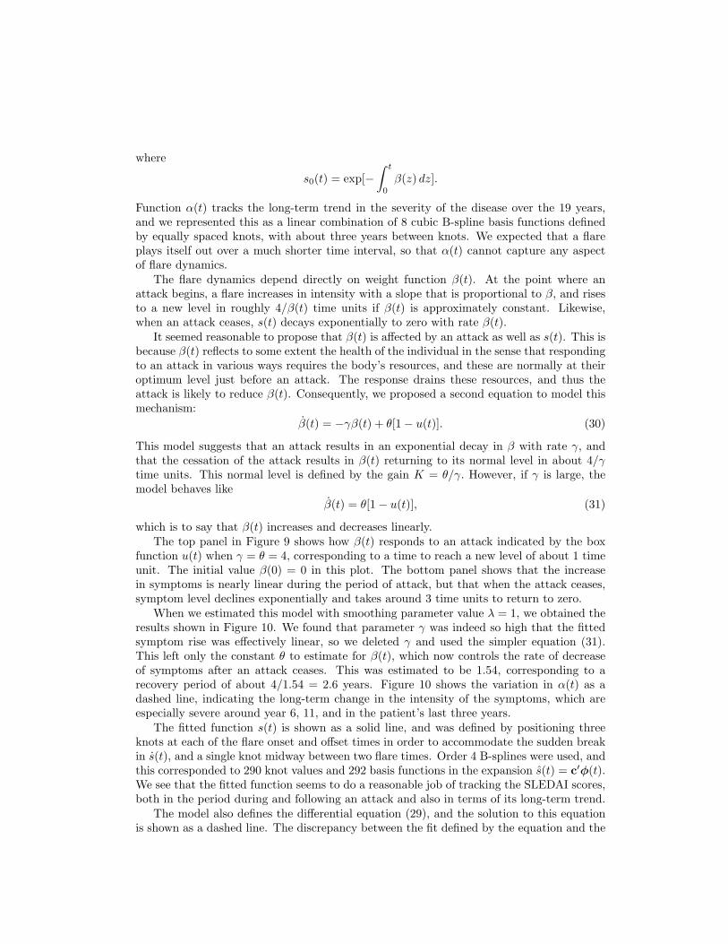
Function α(t) tracks the long-term trend in the severity of the disease over the 19 years,and we represented this as a linear combination of 8 cubic B-spline basis functions definedby equally spaced knots, with about three years between knots. We expected that a flareplays itself out over a much shorter time interval, so that α(t) cannot capture any aspectof flare dynamics.

The flare dynamics depend directly on weight function β(t). At the point where anattack begins, a flare increases in intensity with a slope that is proportional to β, and risesto a new level in roughly 4/β(t) time units if β(t) is approximately constant. Likewise,when an attack ceases, s(t) decays exponentially to zero with rate β(t).

It seemed reasonable to propose that β(t) is affected by an attack as well as s(t). This isbecause β(t) reflects to some extent the health of the individual in the sense that respondingto an attack in various ways requires the body’s resources, and these are normally at theiroptimum level just before an attack. The response drains these resources, and thus theattack is likely to reduce β(t). Consequently, we proposed a second equation to model thismechanism:

β(t) = −γβ(t) + θ[1− u(t)]. (30)

This model suggests that an attack results in an exponential decay in β with rate γ, andthat the cessation of the attack results in β(t) returning to its normal level in about 4/γtime units. This normal level is defined by the gain K = θ/γ. However, if γ is large, themodel behaves like

β(t) = θ[1− u(t)], (31)

which is to say that β(t) increases and decreases linearly.The top panel in Figure 9 shows how β(t) responds to an attack indicated by the box

function u(t) when γ = θ = 4, corresponding to a time to reach a new level of about 1 timeunit. The initial value β(0) = 0 in this plot. The bottom panel shows that the increasein symptoms is nearly linear during the period of attack, but that when the attack ceases,symptom level declines exponentially and takes around 3 time units to return to zero.

When we estimated this model with smoothing parameter value λ = 1, we obtained theresults shown in Figure 10. We found that parameter γ was indeed so high that the fittedsymptom rise was effectively linear, so we deleted γ and used the simpler equation (31).This left only the constant θ to estimate for β(t), which now controls the rate of decreaseof symptoms after an attack ceases. This was estimated to be 1.54, corresponding to arecovery period of about 4/1.54 = 2.6 years. Figure 10 shows the variation in α(t) as adashed line, indicating the long-term change in the intensity of the symptoms, which areespecially severe around year 6, 11, and in the patient’s last three years.

The fitted function s(t) is shown as a solid line, and was defined by positioning threeknots at each of the flare onset and offset times in order to accommodate the sudden breakin s(t), and a single knot midway between two flare times. Order 4 B-splines were used, andthis corresponded to 290 knot values and 292 basis functions in the expansion s(t) = c′φ(t).We see that the fitted function seems to do a reasonable job of tracking the SLEDAI scores,both in the period during and following an attack and also in terms of its long-term trend.

The model also defines the differential equation (29), and the solution to this equationis shown as a dashed line. The discrepancy between the fit defined by the equation and the


0 0.5 1 1.5 2 2.5 3 3.5 4 4.5 50

0.5

1

1.5

2

β(t)

0 0.5 1 1.5 2 2.5 3 3.5 4 4.5 50

1

2

3

4

t

s(t)

Fig. 9. The top panel shows the effect of a lupus attack on the weight function β(t) in differentialequation (29). The bottom panel shows the time course of the symptom severity function s(t).

0 2 4 6 8 10 12 14 16 180

5

10

15

20

25

Year

SLE

DAI s

core

Fig. 10. The circles indicate SLEDAI scores, the jagged solid line is the smoothing functions s(t),the dashed jagged line is the solution to the differential equation and the smooth dashed line is thesmooth trend α(t).

smoothing function s(t) is important in years 8 to 11, where the equation solution over-estimates symptom level. In this region, new flares come too fast for recovery, and thus buildon each other. Nevertheless, the fit to the 208 SLEDAI scores achieved by an investment of9 structural parameters seems impressive for both the smoothing function s(t) and equationsolution, taking into consideration that the SLEDAI score is a rather imprecise measure.Moreover, the model goes a long way to modeling the within-flare dynamics, the generaltrend in the data, and the interaction between flare dynamics and trend.

5. Generalizations and further problems

5.1. More general equationsWe have discussed the methods presented here with respect to systems of ODEs. However,these methods can be applied to the following situations in a direct manner:

• Differential-algebraic equations (DAEs), in which some components of x are specifieddirectly rather than on the derivative scale:

xi(t) = fi(x,u, t|θ). (32)

Such systems are common in chemical engineering; see (Biegler et al. (1986)) for aclassical example.

• Lagged equations:x(t) = f(x(t− δ1),u(t− δ2), t|θ),

where δ1 and δ2 are vectors of time lags for state and forcing functions, respectively.

• Partial differential equations (PDEs)in which a system x(s, t) is described over spatialvariables s as well as time t:

∂x∂t

= f(x,

∂x∂s

,u, t|θ)

.

Both lagged and partial differential equations require the specification of an infinitedimensional boundary condition, rather than a finite set of initial conditions.

5.2. Stochastic differential equationsCriterion (14) may be interpreted as the log likelihood for an observation from the stochasticdifferential equation:

x(t) = f(x,u, t|θ) + λdW(t)

dt

where W(t) is a d-dimensional Brownian motion. Thus for a fixed λ, interpreted as theratio of the Brownian motion variance to that of the observational error, the procedure maybe thought of as profiling an estimate of the realized Brownian motion. This approach hasbeen used for the problem of data assimilation in Apte et al. (2007), where they use criteriaclosely related to our own (14). This notion is appealing and suggests the use of alternativesmoothing penalties based on the likelihood of other stochastic processes. The flares in theLupus data, for example, could be considered to be triggered by events in a Poisson process,and we expect this to be a fruitful area of future research. However, this interpretation


relies on the representation of dW(t)/dt in terms of the discrepancy x(t) − f(x,u, t|θ)where x is given by a basis expansion (7). For nonlinear f the approximation propertiesof this discrepancy are not clear. Moreover, it is frequently the case that lack of fit innonlinear dynamics is due more to mis-specification of the system under consideration thanto stochastic inputs, and we are correspondingly wary of this interpretation.

5.3. Further statistical problemsDiagnostic tools are needed for differential equation models. Particularly in biological appli-cations, these models often provide the right qualitative behavior and may take values ordersof magnitude different from the observed data. Diagnostic analyses can estimate additionalcomponents of u that will provide good fits. These may be correlated with observed valuesof the system, or external factors, to suggest new model formulae.

Experimental design is a relatively unexplored area of research for nonlinear dynamicalsystems. Engineers plan experiments in which inputs are varied under various regimes;including step, ramp, periodic and other perturbations. These inputs are then continuousfunctions which join sampling rates for each component and replicated experiments as designvariables. See Bauer et al. (2000) for an approach to these problems.

Finally, there are a large class of theoretical and inferential problems in fitting nonlineardifferential equations to data, including inference near bifurcation boundaries, about systemstability and on the relationship between statistical information and chaotic behavior.

6. Conclusions

Differential equations have a long and illustrious history in mathematical modeling. How-ever, there has been little development of statistical theory for estimating such models orassessing their agreement with observational data. Our approach, a variety of collocationmethod, combines the concepts of smoothing and estimation, providing a continuum oftrade-offs between fitting the data well and fidelity to the hypothesized differential equa-tions. This has been done by defining a fit through a penalized spline criterion for eachvalue of θ and then estimating θ through a profiling scheme in which the fit is regarded asa nuisance parameter.

We have found that this procedure has a number of important advantages relative toolder methods such as nonlinear least squares. Parameter estimates can be obtained fromdata on partially measured systems, a common situation where certain variables are expen-sive to measure or are intrinsically latent. Comparisons with other approaches suggest thatthe bias and sampling variance of these estimates is at least as good as for other approaches,and rather better relative to methods such as NLS. The sampling variation in the estimatesis easily estimable, and our simulation experiments and experience indicate that there isgood agreement between these estimation precision indicators and the actual estimation ac-curacies. Our approach also gains from not requiring a formulation of the dynamic model asan initial value problem in situations where initial values are not available or not required.

On the computational side, the algorithm is as fast or faster than NLS and other ap-proaches. Unlike Bayesian MCMC, the generalized profiling approach is relatively straight-forward to deploy to a wide range of applications, and software in Matlab described belowmerely requires that the user to code the various partial derivatives that are involved, andwhich are detailed in the Appendix. Finally, the method is also robust in the sense of con-verging over a wide range of starting parameter values. The possibility of beginning with

smaller values of λ so as to work with a smooth criterion, and then stepping these valuesup toward those defining near approximations to the ODE further adds to the method’srobustness.

Finally the fitting of a compromise between an actual ODE solution and a simple smoothof the data adds a great deal of flexibility that should prove useful to users wishing to explorevariation in the data not representable in the ODE model. By comparing fits with smallervalues of λ with fits that are near or exact ODE solutions, the approach offers a diagnosticcapability that can guide further extensions and elaborations of the model.

6.1. SoftwareAll the results in this paper have been generated in the MATLAB computing language,making use of functional data analysis software intended to compliment Ramsay and Sil-verman (2005). A set of software routines that may be applied to any differential equationis available from the URL: http://www.functionaldata.org.

References

Apte, A., M. Hairer, A. M. Stuart, and J. Voss (2007). Sampling the posterior: An approachto non-gaussian data assymilation. Physica D, to appear.

Arora, N. and L. T. Biegler (2004). A trust region SQP algorithm for equality constrainedparameter estimation with simple parametric bounds. Computational Optimization andApplications 28, 51–86.

Bates, D. M. and D. B. Watts (1988). Nonlinear Regression Analysis and Its Applications.New York: Wiley.

Bauer, I., H. G. Bock, S. Korkel, and J. P. Schloder (2000). Numerical methods for optimumexperimental design in DAE systems. Journal of Computational and Applied Mathemat-ics 120, 1–25.

Biegler, L., J. J. Damiano, and G. E. Blau (1986). Nonlinear parameter estimation: a casestudy comparison. AIChE Journal 32 (1), 29–45.

Biegler, L. and I. Grossman (2004). Retrospective on optimization. Computers and ChemicalEngineering 28, 1169–1192.

Bock, H. G. (1983). Recent advances in parameter identification techniques for ODE.In P. Deuflhard and E. Harrier (Eds.), Numerical Treatment of Inverse Problems inDifferential and Integral Equations, pp. 95–121. Basel: Birkhauser.

Campbell, D. (2007). Bayesian Collocation Tempering and Generalized Profiling for Estima-tion of Parameters From Differential Equation Models. Ph. D. thesis, McGill University.

Campbell, D., G. Hooker, J. O. Ramsay, K. McAuley, and J. McLellan (2007). Generalizedprofiling parameter estimation in differential equation models with constrained variables.unpublished manuscript.

Cao, J. and J. O. Ramsay (2006). Parameter cascades and profiling in functional dataanalysis. Computational Statistics, In press.


Cox, D. R. and D. V. Hinkley (1974). Theoretical Statistics. London: Chapman & Hall.

Denis-Vidal, L., G. Joly-Blanchard, and C. Noiret (2003). System identifiability (sym-bolic computation) and parameter estimation (numerical computation). Numerical Al-gorithms 34, 283–292.

Deuflhard, P. and F. Bornemann (2000). Scientific Compuitng with Ordinary DifferentialEquations. New York: Springer-Verlag.

Esposito, W. R. and C. Floudas (2000). Deterministic global optimization in nonlinearoptimal control problems. Journal of Global Optimization 17, 97–126.

FitzHugh, R. (1961). Impulses and physiological states in models of nerve membrane.Biophysical Journal 1, 445–466.

Friedman, J. and B. W. Silverman (1989). Flexible parsimonious smoothing and additivemodeling. Technometrics 3, 3–21.

Gelman, A., F. Y. Bois, and J. Jiang (1996). Physiological pharmacokinetic analysis us-ing population modeling and informative prior distributions. Journal of the AmericanStatistical Association 91 (436), 1400–1412.

Hodgkin, A. L. and A. F. Huxley (1952). A quantitative description of membrane currentand its application to conduction and excitation in nerve. J. Physiol. 133, 444–479.

Hooker, G. (2007). Theorems and calculations for smoothing-based profiled estimation ofdifferential equations. Technical Report BU-1671-M, Dept. Bio. Stat. and Comp. Bio.,Cornell University.

Jaeger, J., M. Blagov, D. Kosman, K. Kolsov, Manu, E. Myasnikova, S. Surkova, C. Vanario-Alonso, M. Samsonova, D. Sharp, and J. Reinitz (2004). Dynamical analysis of regulatoryinteractions in the gap gene system of drosophila melanogaster. Genetics (167), 1721–1737.

Keilegom, I. V. and R. J. Carroll (2006). Backfitting versus profiling in general criterionfunctions. Submitted to Statistica Sinica.

Koenker, R. and I. Mizera (2002). Elastic and plastic splines: Some experimental compar-isons. In Y. Dodge (Ed.), Statistical Data Analysis based on the L1-norm and RelatedMethods, pp. 405–414. Basel: Birkhauser.

Marlin, T. E. (2000). Process Control. New York: McGraw-Hill.

Nagumo, J. S., S. Arimoto, and S. Yoshizawa (1962). An active pulse transmission linesimulating a nerve axon. Proceedings of the IRE 50, 2061–2070.

Poyton, A. A., M. S. Varziri, K. B. McAuley, P. J. McLellan, and J. O. Ramsay (2006).Parameter estimation in continuous dynamic models using principal differential analysis.Computational Chemical Engineering 30, 698–708.

Ramsay, J. O. and B. W. Silverman (2005). Functional Data Analysis. New York: Springer.

Seber, G. A. F. and C. J. Wild (1989). Nonlinear Regression. New York: Wiley.

Tjoa, I.-B. and L. Biegler (1991). Simultaneous solution and optimization strategies forparameter estimation of differential-algebraic equation systems. Industrial Engineeringand Chemical Research 30, 376–385.

Varah, J. M. (1982). A spline least squares method for numerical parameter estimation indifferential equations. SIAM Journal on Scientific Computing 3, 28–46.

Wahba, G. (1990). Spline Models for Observational Data. Philadelphia: SIAM CBMS-NSFRegional Conference Series in Applied Mathematics.

Wilson, H. R. (1999). Spikes, Decisions and Actions: The Dynamical Foundations of Neu-roscience. Oxford: Oxford University Press.

Zheng, W., K. McAuley, K. Marchildon, and K. Z. Yao (2005). Effects of end-group balanceon melt-phase nylon 612 polycondensation: Experimental study and mathematical model.Ind. Eng. Chem. Res. 44, 2675–2686.


Appendices

A. Matrix calculations for pro�ling

The calculations used throughout this paper have been based on matrices defined in termsof derivatives of F and H with respect to θ and c. In many cases, these matrices are non-trivial to calculate and expressions for their entries are derived here. For these calculations,we have assumed that the outer criterion, F is a straight-forward weighted sum of squarederrors and only depends on θ through x.

A.1. Inner optimizationUsing a Gauss-Newton method, we require the derivative of the fit at each observationpoint:

dxi(t)dci

= φi(t)

where matrix φi is the vector corresponding to the evaluation of all the basis functions usedto represent xi evaluated at t. This gradient of xi with respect to cj is zero.

A numerical quadrature rule allows the set of errors to be augmented with the evaluationof the penalty at the quadrature points and weighted by the quadrature rule:

(λivq)1/2 (xi(tq)− fi(x(tq),u(tq), tq|θ)) .

Each of these then has derivative with respect to cj :

(λivq)1/2 (xi(tq)− fi(x(tq),u(tq), tq|θ)) I(i = j)φi(tq)

−(

n∑

k=1

(λivq)1/2 dfk

dxj(Dxi(tq)− fi(x(tq),u(tq), tq|θ))

)φj(tq)

and the augmented errors and gradients can be used in a Gauss-Newton scheme. I(·) isused as the indicator function of its argument.

A.2. Estimating structural parametersAs in the inner optimization, in employing a Gauss-Newton scheme, we merely need towrite a gradient for the point-wise fit with respect to the parameters:

dx(t)dθ

=dx(t)dc

dcdθ

where dx(ti)/dc has already be calculated and

dcdθ

= −[d2H

dc2

]−1d2H

dcdθ

by the implicit function theorem.

The Hessian matrix d2H/dc2 may be expressed as a block form, the (i, j)th block cor-responding to the cross-derivatives of the coefficients in the ith and jth components of x.This block’s (p, q)th entry is given by:

(ni∑

k=1

φip(t)φjq(t) + λ

∫φip(t)φjq(t)dt

)I(i = j)

− λi

∫φip(t)

dfi

dxjφjq(t)dt− λj

∫φip(t)

dfi

dxjφjq(t)dt

+∫

φip(t)

[n∑

k=1

λk

(d2fk

dxidxj(fk − xk(t)) +

dfk

dxi

dfk

dxj

)]φjq(t)dt

with the integrals evaluated by numeric integration. The arguments to fk(x,u, t|θ) havebeen dropped in the interests of notational legibility.

We can similarly express the cross-derivatives d2H/dcdθ as a block vector, the ith blockcorresponding to the coefficients in the basis expansion for the ith component of x. Thepth entry of this block can now be expressed as:

λi

∫dfi

dθφip(t)dt−

∫ (n∑

k=1

λk

[d2fk

dxidθ(fk − xk(t)) +

dfk

dxi

dfk

dθ

])φip(t)dt.

A.3. Estimating the variance of θThe variance of the parameter estimates is calculated using

dθ

dy= −

[d2H

dθ2

]−1d2H

dθdy,

where

d2H

dθ2 =∂2H

∂θ2 +(

∂c∂θ

)′∂2H

∂c∂θ+

∂2H

∂θ∂c∂c∂θ

+(

∂c∂θ

)′∂2H

∂c2

∂c∂θ

+∂H

∂c∂2c∂θ2 , (33)

andd2H

dθdy=

∂2H

∂θ∂y+

∂2H

∂c∂y∂c∂θ

+∂2H

∂θ∂c∂c∂y

+∂2H

∂c2

∂c∂y

∂c∂θ

+∂H

∂c∂2c

∂θ∂y. (34)

The formulas (33) and (34) for d2H/dθ2 and d2H/dθdy involve the terms ∂c/∂y, ∂2c/∂θ2

and ∂2c/∂θ∂y. In the following, we derive their analytical formulas by the Implicit FunctionTheorem. We introduce the following convention, which is called Einstein SummationNotation. If a Latin index is repeated in a term, then it is understood as a summation withrespect to that index. For instance, instead of the expression

∑i aixi, we merely write aixi.

• ∂c∂ySimilar as the deduction for dc/dθ, we obtain the formula for ∂c/∂y by applying theImplicit Function Theorem:

∂c∂y

= −[∂2J(c|θ,y)

∂c2

∣∣∣∣c

]−1[∂2J(c|θ,y)

∂c∂y

∣∣∣∣c

]. (35)


• ∂c2

∂θ∂yBy taking the second derivative on both sides of the identity ∂J(c|θ,y)/∂c|c = 0 withrespect to θ and yk, we derive:

d2

dθdyk

(∂J(c|θ,y)

∂c

∣∣∣∣c

)∂3J(c|θ,y)∂c∂θ∂yk

∣∣∣∣c

+∂3J(c|θ,y)∂c∂θ∂ci

∣∣∣∣c

∂ci

∂yk

+∂3J(c|θ,y)

∂c2∂yk

∣∣∣∣c

∂c∂θ

+∂3J(c|θ,y)

∂c2∂ci

∣∣∣∣c

∂ci

∂yk

∂c∂θ

+∂2J(c|θ,y)

∂c2

∣∣∣∣c

∂2c∂θ∂yk

. (36)

Solving for ∂2c∂θ∂yk

, we obtain the second derivative of c with respect to θ and yk:

∂2c∂θ∂yk

= −[∂2J(c|θ,y)

∂c2

∣∣∣∣c

]−1[∂3J(c|θ,y)∂c∂θ∂yk

∣∣∣∣c


∣∣∣∣c

∂ci

∂yk

+∂3J(c|θ,y)

∂c2∂yk

∣∣∣∣c

∂c∂θ

+∂3J(c|θ,y)

∂c2∂ci

∣∣∣∣c

∂ci

∂yk

∂c∂θ

]. (37)

• ∂2c∂θ2

Similar to the deduction of ∂2c/∂θ∂yk, the second partial derivative of c with respectto θ and θj is:

∂2c∂θ∂θj

= −[∂2J(c|θ,y)

∂c2

∣∣∣∣c

]−1[∂3J(c|θ,y)∂c∂θ∂θj

∣∣∣∣c


∣∣∣∣c

∂ci

∂θj

+∂3J(c|θ,y)

∂c2∂θj

∣∣∣∣c

∂c∂θ

+∂3J(c|θ,y)

∂c2∂ci

∣∣∣∣c

∂ci

∂θj

∂c∂θ

]. (38)

When estimating ODEs, we define J(c|θ,y) as (14) and H(θ, c(θ)|y) as (8), and furtherwrite the above formulas in terms of the basis functions in φ and the functions f on theright side of the differential equation. For instance, d2H/dc2 is a block-diagonal matrixwith the ith block being wiφi(ti)T φi(ti) and dF/dc is a block vector containing blocks−wiφi(ti)T (yi − xi(ti)).

The three-dimensional array ∂3J/∂c∂cp∂cq can be written in the same block vector formas ∂2J/∂c∂θ with the uth entry of the kth block given by

∫ (n∑

l=1

λl

[d2fl

dxidxj

dfl

dxk+

d2fl

dxidxk

dfl

dxj+

d2fl

dxjdxk

dfl

dxi

])φip(t)φjq(t)φku(t)dt

+∫ n∑

l=1

λl

(d3fk

dxidxjdxk(fl − xl(t))

)φip(t)φjq(t)φku(t)dt

− λi

∫d2fi

dxjdxkφip(t)φjq(t)φku(t)dt− λj

∫d2fj

dxidxkφip(t)φjq(t)φku(t)dt

− λk

∫d2fk

dxidxjφip(t)φjq(t)φku(t)dt

assuming cp is a coefficient in the basis representation of xi and cq a corresponds to xj . Thearray ∂3J/∂c∂θi∂θj is also expressed in the same block form with entry p in the kth block

being:

∫ (n∑

l=1

λl

[d2fl

dθidθj

dfl

dxk+

d2fl

dθidxk

dfl

dθj+

d2fl

dθjdxk

dfl

dθi

])φkp(t)dt

+∫ n∑

l=1

λl

(d3fk

dxkdθidθj(fl − xl(t))

)φkp(t)dt− λk

∫d2fk

dθidθkφkp(t)dt.

The term ∂3J/∂c∂cp∂θi is in the same block from, with the qth entry of the jth block being:

∫ (n∑

l=1

λl

[d2fl

dθidxj

dfl

dxk+

d2fl

dθidxk

dfl

dxj+

d2fl

dxjdxk

dfl

dθi

])φkp(t)φjq(t)dt

+∫ n∑

l=1

λl

(d3fk

dxjdxkdθi(fl − xl(t))

)φkp(t)φjq(t)dt

− λj

∫d2fj

dθidxkφjq(t)φkp(t)dt− λk

∫d2fk

dθidxjφjq(t)φkp(t)dt

where cp corresponds to the basis representation of xk.Similar calculations give matrix d2H/dθdy explicitly as:

dcdθ

T [∂2H

∂c∂y+

∂2H

∂c2

dcdy

]

− ∂H

∂c

[∂2H

∂c2

]−1{

N∑p,q=1

dcp

dθ

T ∂3J

∂c∂cp∂cq

dcq

dy+

N∑p=1

∂3J

∂c∂cp∂θ

dcp

dy

}

with dc/dy given by

−[∂2J

∂c2

]−1∂2J

∂c∂y

and ∂2J/∂cdy being block diagonal with the ith block containing wiφi(ti).

Parameter Estimation for Differential Equations: A Gen- eralized...

Documents

Transcript of Parameter Estimation for Differential Equations: A Gen- eralized...