Parameter and State Estimation using Audio and Video Signals · 2005-11-09 · Parameter and State...
110
IT Licentiate theses 2005-009 Parameter and State Estimation using Audio and Video Signals M AGNUS E VESTEDT UPPSALA UNIVERSITY Department of Information Technology
Transcript of Parameter and State Estimation using Audio and Video Signals · 2005-11-09 · Parameter and State...

IT Licentiate theses2005-009
Parameter and State Estimation usingAudio and Video Signals
MAGNUS EVESTEDT
UPPSALA UNIVERSITYDepartment of Information Technology

Parameter and State Estimation using Audio andVideo Signals
BY
MAGNUS EVESTEDT
November 2005
DIVISION OF SYSTEMS AND CONTROL
DEPARTMENT OFINFORMATION TECHNOLOGY
UPPSALA UNIVERSITY
UPPSALA
SWEDEN
Dissertation for the degree of Licentiate of Philosophy in Electrical Engineering withSpecialization in Automatic Control
at Uppsala University 2005
Parameter and State Estimation using Audio and Video Signals
Magnus Evestedt
Division of Systems and ControlDepartment of Information Technology
Uppsala UniversityBox 337
SE-751 05 UppsalaSweden
http://www.it.uu.se/
c© Magnus Evestedt 2005ISSN 1404-5117
Printed by the Department of Information Technology, Uppsala University, Sweden

Abstract
The complexity of industrial systems and the mathematical models to de-scribe them increases. In many cases point sensors are no longer sufficientto provide controllers and monitoring instruments with the information nec-essary for operation. The need for other types of information, such as audioand video, has grown. Suitable applications range in a broad spectrum frommicroelectromechanical systems and bio-medical engineering to papermak-ing and steel production.
This thesis is divided into five parts. First a general introduction to thefield of vision-based and sound-based monitoring and control is given. Adescription of the target application in the steel industry is included.
In the second part, a recursive parameter estimation algorithm that does notdiverge under lack of excitation is studied. The focus is on the stationaryproperties of the algorithm and the corresponding Riccati equation.
The third part compares the parameter estimation algorithm to a numberof well-known estimation techniques, such as the Normalized Least MeanSquares and the Kalman filter. The benchmark for the comparison is anacoustic echo cancellation application. When the input is insufficiently ex-citing, the studied method performs best of all considered schemes.
The fourth part of the thesis concerns an experimental application of vision-based estimation. A water model is used to simulate the behaviour of thesteel bath in a Linz-Donawitz steel converter. The water model is capturedfrom the side by a video camera. The images together with a nonlinearmodel is used to estimate important process parameters, describing the heatand mass transport in the process. The estimation results are compared tothose obtained by previous researchers and the suggested approach is shownto decrease the estimation error variance by 50%.
The complexity of the parameter estimation procedure by means of opti-mization makes the computation time large. In the final part, the timeconsumption of the estimation is decreased by using a smaller number ofdata points. Three ways of choosing the sampling points are considered. Anobserver- based approach decreases the computation time significantly, withan acceptable loss of accuracy of the estimates.
List of publications
I: Evestedt Magnus and Alexander Medvedev, Stationary behaviour ofan anti-windup scheme for recursive parameter estimation under lackof excitation, To appear in Automatica, January, 2006.
A conference version was published in:
Evestedt Magnus and Alexander Medvedev, Stationary behaviour ofan anti-windup scheme for recursive parameter estimation under lackof excitation, Proceedings of the 16th IFAC World Congress, July 4-8,2005, Prague, Czech Republic.
II: Evestedt Magnus, Alexander Medvedev and Torbjorn Wigren, Windupproperties of recursive parameter estimation algorithms in acousticecho cancellation, Revised version submitted to Control EngineeringPractice.
Conference versions of the paper were published in:
Evestedt Magnus, Alexander Medvedev and Torbjorn Wigren, Windupproperties of recursive parameter estimation algorithms in acousticecho cancellation, Proceedings of the 16th IFAC World Congress, July4-8, 2005, Prague, Czech Republic.
Evestedt Magnus, Alexander Medvedev and Torbjorn Wigren, Com-parative study of three recursive parameter estimation algorithms withapplication to echo cancellation, Reglermote 2004, May 26-27, 2004,Gothenburg, Sweden.
III: Evestedt Magnus and Alexander Medvedev, Gas jet impinging on liq-uid surface: Cavity spaciotemporal modelling and estimation, Submit-ted.
Parts of the material were published in:
Evestedt Magnus and Alexander Medvedev, Gas jet impinging on liq-uid surface: Cavity shape modelling and video based estimation, Pro-ceedings of the 16th IFAC World Congress, July 4-8, 2005, Prague,Czech Republic.
Evestedt Magnus and Alexander Medvedev, Cavity depth and diam-eter estimation in the converter process water model, Association forIron & Steel Technology Conference Proceedings, pp.763-771, Septem-ber 15-17, 2004, Nashville, Tennessee, USA.
IV: Evestedt Magnus and Alexander Medvedev, Model-based cavity shapeestimation in a gas-liquid system with nonuniform image sampling.Submitted.

Acknowledgments
I would like to thank my supervisor Professor Alexander Medvedev for hisguidance and enthusiasm over the last couple of years. I would also like tothank my colleagues at the Division of Systems and Control for the smilesand laughs we share at work. Finally, I would like to extend a big hug tomy friends and family. Osu!


Summary 1
1 Introduction
Imagine what it would be like not being able to see. Or hear. You wouldhave to rely on your other senses, like touch, taste and smell. Eating agood meal would be easy using those sensors, but what if you would have toprepare the meal yourself? That task is more complex and would probablybe more problematic to perform.
The industry has for a long time relied on point sensors to measure forexample temperature or pressure in a process. Due to the increasing com-plexity of industrial systems and the models used to describe them, othertypes of information are needed for monitoring and control. In many casesmeasurements obtained by means of image capturing and audio can providethe necessary information. Images can be either conventional (captured byfor example a CCD camera), reconstructed (magnetic resonance images),[8], or abstract (sensor data represented as an image). Suitable applicationsrange in a broad spectrum from microelectromechanical systems (MEMS)and bio-medical engineering to papermaking and steel production.
Audio signals occur in many applications, such as echo cancellation, non-destructive material testing, process control and monitoring in e.g. the steelindustry. A close connection between audio signals and images can be found,for instance, in medicine where ultrasonic waves are used to reconstructimages of internal organs of the human body.
The topics of vision-based and audio-based monitoring and control are com-monly treated in the context of robotics and autonomous systems. Visionis required to aid the navigation, grasping, placing, steering and motion ofa machine, be it a robot arm, a vehicle or any other mechanical mechanism.Hearing is needed for interaction between a human and the robot and forlocalizing the source of sound. The first robotic systems incorporating videoappeared in 1970, [17]. The area has developed immensely since then andhas provided means for reconstruction of camera motion, scene structureand camera self calibration.
The applications in process technology and bio-medicine are, however, dif-ferent compared to robotics. Firstly, video is often used together withother sensors and secondly the process parameters observed by video areseldom the ones to be monitored. Thus, a model-based estimation algo-rithm must be used to extract the information of interest from the availabledata. Thirdly the mathematical models of industrial processes, biologicaland medical systems are typically uncertain and empiric, which makes thedesign of vision-based control systems a very challenging task.

2 Magnus Evestedt
1.1 Image processing
When an image is captured by a CCD camera, a discrete two-dimensionalrepresentation of the real world scene is created. The CCD image consists ofa gray-level array of pixels (picture elements) describing the light intensityand color of the scene. The imaging process can be seen as a transformationbetween spaces of different dimensions (3D→ 2D) and information is lostin the process. However, the amount of redundant information in the pixelarray is typically large, due to the large number of pixels in an image.The information contribution of each picture element is very low, but sinceneighboring pixels are highly dependent, the redundancy can be exploitedto extract valuable data from the image. Image processing can be dividedinto pixel-based methods and model-based methods. In the following, thetwo concepts are explained further. Numerous text books have been writtenin the area of image analysis, for example [15, 34].
1.1.1 Pixel-based methods
As a first step in the image processing chain, techniques for image enhance-ment and image restoration might be used. The image enhancement oper-ations include gray-level transformations, histogram processing, smoothingand sharpening spatial filters, and various frequency domain methods. Inimage restoration, filters are utilized to reduce the noise by for examplefrequency domain operations.
The second step is to extract information from the image using feature ex-traction. This is a procedure to divide the image into regions with differ-ent characteristics. The result of such an operation is a segmented image.Techniques for image segmentation include edge detection, thresholding andadaptive thresholding.
Morphological image processing techniques, such as dilation, erosion, open-ing and closing, [34], are often used in real time applications due to theirlow computational complexity. The operations are used for image pre-processing, object structure enhancement, object segmentation and quanti-tative description of objects (area, perimeter, etc.).

Summary 3
1.1.2 Model-based methods
A model-based approach can instead be used to segment and understand animage. Examples of such operations are active contour models, or snakes,and level set methods, [28]. A snake is defined as an energy minimizing splinewhose energy depends on its shape and location within the image. The localminima of this energy correspond to desired image properties. The searchfor a minimum is a slow process and therefore real-time implementationsare unusual.
1.1.3 Image processing and control
The field of image processing and the field of automatic control have inthe past been kept apart and the interaction between them has been ig-nored. A kind of separation principle has been applied, where the controland vision aspects of a problem are treated independently. Image process-ing alone might not be enough to provide information about the state of anindustrial process, but together with other available sensor measurements itcan become a vital part of control system design. The connection betweencontrol and snakes is obvious. The models used in both fields are (partial)differential equations with few parameters. A typical problem with snakesis the initialization of the active shape and convergence of the optimizationto a local energy minimum. The initialization part should not pose a majordifficulty in control, since the initial shape of the expected image is usuallyknown. Recently, a textbook containing references to industrial applicationsof process imaging was published, [31].
An approach to video monitoring and control of the coal powder injectionin a blast furnace is presented in [6]. A video camera that captures theface of a car driver can be used to detect if the driver is falling asleep bymonitoring the activity of parts of the face, in particular the eyes, [10], [11].In [19] a video camera is used as a sensor for a lane following controller. Anautomatic observation system of the dry line in a paper machine is presentedin [4]. In [27], a combination of force and visual feedback is used to controlan industrial robot.
1.2 Sound processing
There are numerous applications involving sound, mostly in the area ofsignal processing. The transmission of voice over a frequency channel is an

4 Magnus Evestedt
important issue in the cell phone system industry. One of the problems forthe designer of such a system is that of echo cancellation, where the echoof the transmitted speech back to the transmitting end is to be reduced orcancelled, [1, 7, 16].
The applications of sound in the field of automatic control are sparse. Spec-tral analysis methods are often employed to extract valuable informationfrom a microphone signal. Spectral analysis, however, applied in the usualway, is problematic in closed loop, [33].
In [5] a microphone is used to estimate the foam level in a water tank.In [18] microphones are used to control the sound transmission through awindow using feedback control. A non-destructive way to analyze microc-rack formation of a material is acoustic emission. The acoustic emission aresound waves emitted by the cracks as they are created or move. The soundwaves propagate through the material and are recorded by a system thatcontinuously listens at the surface of the sample, [32].
1.3 Modelling and estimation
To be able to analyze, describe and control an industrial process, a math-ematical model of the system is required. The mathematical model can beconstructed in two main ways:
• Mathematical modelling. The model is derived using physical laws,for example Newton’s laws or Maxwell’s laws.
• System identification. Experiments are performed on the studied sys-tem and a model is fitted to the collected data. The model is oftenproposed without exploiting physical laws, black-box modelling.
Combinations of system identification and physical insight are also used tomodel the process, grey-box modelling. The mathematical model might thencontain unknown parameters that need to be estimated using identificationmethods.
The unknown parameters in the model are determined by utilizing experi-mental data from the system. The data are used together with the modeland a suitable parameter estimation algorithm to determine the unknowns.There are many textbooks in the field of parameter estimation and systemidentification, including [22, 30, 33].

Summary 5
1.4 Example: The Linz-Donawitz (LD)-converter
An example of an industrial application where both images as well as soundsignals are used for process monitoring and control is the LD steel converter,Figure 1.
Figure 1: The LD-converter is a hostile environment for performing mea-surements.
The main principle of the LD converter is to convert hot molten iron intosteel by oxidizing the contents of Mn, C, Si and Fe. The oxygen is blownfrom above onto the steel melt and a cavity is formed on the liquid surface.The chemical reactions take place both in the cavity and in the foam or slagthat is produced in the process. The slag contains bubbles and provides alarge surface area for the oxidization. The depth and diameter of the cavity,determining heat and mass transport at the interface and in the liquid, areimportant parameters in the process.

6 Magnus Evestedt
An investigation of the possibilities of automation in the steelmaking processwas presented in [37]. The height of the lance and the gas flow rate of theoxygen are the main process variables used to control the process. Theavailable measurements that provide real-time information on the state ofthe process are off-gas analysis, sound level measurement with a microphone(sonic-meter) and off-gas temperature. The sonic meter is located in thehood above the converter mouth and is used as a monitoring instrument forthe operators, indicating changes in slag level.
Since the inside of the LD converter is a highly hostile environment, the formof the cavity is difficult to observe in the actual process. For the purposeof studying the form of the cavity, physical models are often employed,providing far more beneficial experimental conditions. The physical modelconsists of a tank filled with a liquid (e.g. water, mercury) and a lancethrough which gas (e.g. oxygen, argon, nitrogen) is blown onto the liquidsurface. A video camera, facing the tank from the side, is used to monitorthe liquid deformation during the blow.
In [5] a microphone was placed above a water tank recording the noise fromthe blow. The audio signal was used to estimate and control the level offoam in the water model by changing the height of the lance and the air flowthrough the lance.
The problem of modelling the cavity and estimation of its form is long-standing in metallurgy and has been studied since the early 1960´s [2, 3,9, 12, 13, 20, 21, 23, 24, 25, 26, 29, 35, 36]. The analytical results havealways been compared to photographs obtained experimentally, either withthe water model or a similar physical model. A ruler was often used tomeasure the cavity characteristics and the uncertainty of the measurementswas never commented upon. It is not until recent years that the idea ofactually combining image processing techniques and model based parame-ter estimation have been utilized to further the knowledge of the converterprocess, [12, 13, 14].
1.5 Thesis Outline
The following is an outline of the content and contributions of this thesis.
I: In some systems, the excitation in the input signal might sometimesbecome insufficient for system identification. If a Kalman filter isused as a parameter estimator, the insufficient excitation leads to an

Summary 7
increase of the eigenvalues, so called wind-up, of the matrix in the so-lution to the Riccati equation. In this paper the stationary propertiesof an algorithm for wind-up prevention, obtained by a specialization ofthe Kalman filter algorithm, are investigated. The algorithm is shownto possess good anti-windup properties.
II: The windup properties of a recursive parameter estimation algorithm,obtained by a specialization of the Kalman filter, are compared to anumber of well-known estimation techniques, such as the NormalizedLeast Mean Squares and the Kalman filter. An acoustic echo cancel-lation application is used as a benchmark for the comparison. Theconvergence and estimation accuracy of the new approach are close tothe Kalman filter performance. With insufficient input excitation, themethod performs best of all considered estimation schemes.
III: In this paper a water model is studied to simulate physical phenomenain the LD steel converter. A CCD camera is used to capture the watertank from the side. A mathematical model, together with the videosequence, is used to describe the cavity form in the water tank andspecifically estimate the depth and diameter of the surface indentation.The main focus of the paper is on quantification of the uncertainty ofthe estimates obtained under the assumption that the cavity formis constant for a certain choice of gas flow and lance height. Theestimation error variance is shown to decrease by 50% by introducinga model to describe the depth and diameter variations in the timedomain.
IV: A water model is used to experimentally obtain video-based measure-ments of the cavity profile during a blow. A nonlinear model is fittedto the data by tuning model parameters. Three ways of choosing sam-pling points for the optimization procedure are proposed in this paper.The estimation accuracy, data utilization and computation time arecompared. An observer-based method decreases the computation timesubstantially with an acceptable loss of accuracy of the estimates.
References
[1] P. Ahgren. On system identification and acoustic echo cancellation.Ph. D. Thesis Uppsala Dissertations from the Faculty of Science andTechnology: 53, Uppsala University, 2004.
[2] R. B. Banks and D. V. Chandrasekhara. Experimental investigationof the penetration of a high-velocity gas jet through a liquid surface.Journal of Fluid Mechanics, 15(103):13–34, 1963.

8 Magnus Evestedt
[3] J. Berghmans. Theoretical investigation of the interfacial stability ofinviscid fluids in motion, considering surface tension. Journal of FluidMechanics, 54:129–141, 1972.
[4] J. Berndtson and A. J. Niemi. Automatic observation of the dry linein paper machine. In Proceedings of the 13th international conferenceon pattern recognition, volume 3, pages 308–312, August 1996.
[5] W. Birk, I. Arvanitidis, P. Jonsson, and A. Medvedev. Foam level con-trol in a water model of the LD converter process. Control EngineeringPractice, 11:49–56, 2003.
[6] W. Birk, O. Marklund, and A. Medvedev. Video monitoring of pulver-ized coal injection in the blast furnace. IEEE Transactions on IndustryApplications, 38(2), 2002.
[7] C. Breining, P. Dreiseitel, E. Hansler, A. Mader, B. Nitsch, H. Puder,T. Schertler, G. Schmidt, and J. Tilp. Acoustic echo control. IEEESignal Processing Magazine, December 1999.
[8] M. A. Brown and R. C. Semelka. MRI:Basic Principles and Applica-tions. Wiley, 2003.
[9] F. R. Cheslak, J. A. Nicholls, and M. Sichel. Cavities formed on liquidsurfaces by impinging gaseous jets. Journal of Fluid Mechanics, 36:55–64, 1969.
[10] H. J. Dikkers, M. A. Spaans, D. Datcu, M. Novak, and L. J. M.Rothkrantz. Facial recognition system for driver vigilance monitor-ing. In Conference Proceedings - IEEE International Conference onSystems, Man and Cybernetics, October 2004.
[11] T. D’Orazio, M. Leo, and A. Distante. Eye detection in face imagesfor a driver vigilance system. In IEEE Intelligent Vehicles Symposium,Proceedings, October 2004.
[12] S. Eletribi, D. K. Mukherjee, and V. Prasad. Experiments on liquidsurface deformation upon impingement by a gas jet. In Proceedings ofthe ASME Fluids Engineering Division, volume 244, 1997.
[13] M. Evestedt and A. Medvedev. Cavity depth and diameter estima-tion in the converter process water model,. In Association for Iron& Steel Technology Conference Proceedings, pages 763–771, Nashville,Tennessee, USA, September 2004.
[14] M. Evestedt and A. Medvedev. Gas jet impinging on liquid surface:Cavity shape modelling and video-based estimation. In Proceedings ofthe 16th IFAC World Congress, July 2005.

Summary 9
[15] R. C. Gonzales and R. E. Woods. Digital Image Processing. Addison& Wesley, 2002.
[16] E. Hansler. The hands-free telephone problem-an annotated bibliogra-phy. Signal Processing, 27(3):259–271, 1992.
[17] J. Hill and W. T. Park. Real time control of a robot with mobile camera.In 9th ISIR, March 1979.
[18] O. Kaiser, S. Pietrzko, and M. Morari. Feedback control of soundtransmission through a double glazed window. Journal of Sound andVibration, 263(4):775–795, June 2003.
[19] A. Konur, C. H. Unyelioglu, and U Ozguner. Design and stabilityanalysis of a lane following controller. IEEE Transactions on ControlSystems Technology, 5(1), 1997.
[20] S. C. Koria and K. W. Lange. Penetrability of impinging gas jets inmolten steel bath. Steel Research, (9), 1987.
[21] M. S. Lee, S. L. O´Rourke, and N. A. Molloy. Fluid flow and surfacewaves in the BOF. ISS Transactions, 29(10):56–65, 2002.
[22] L. Ljung and T. Soderstrom. Theory and practice of recursive identifi-cation. MIT Press, 1983.
[23] N. A. Molloy. Impinging jet flow in a two-phase system:the basic flowpattern. Journal of the iron and steel institute, pages 943–950, October1970.
[24] A. Nordquist. A physical modeling study of top blowing with focus onthe penetration region. Licentiate thesis, Royal institute of technology,Stockholm, Sweden, 2005.
[25] V. B. Okhotskii. Interaction of impinging gas jet with the bath. Izv.vuzov. Chern. Metallurgia, (4), 1997. In Russian.
[26] W. E. Olmstead and S. Raynor. Depression of an infinite liquid surfaceby an incompressible gas jet. Journal of Fluid Mechanics, 19:561–576,1964.
[27] T. Olsson, R. Johansson, and A. Robertsson. Flexible force-vision con-trol for surface following using multiple cameras. In Proceedings of 2004IEEE/RSJ International Conference on Intelligent Robots and Systems,IROS 2004, Sendai, Japan, October 2004.
[28] S. Osher and R. Fedkiw. Level set methods and dynamic implicit sur-faces. Springer, 2003.
10 Magnus Evestedt
[29] R. S. Rosler and G. H. Stewart. Impingement of gas jets on liquidsurfaces. Journal of Fluid Mechanics, 31:163–174, 1968.
[30] A. H. Sayed. Fundamentals of adaptive filtering. Wiley-Interscience,2003.
[31] D. M. Scott and H. McCann. Process imaging for automatic control.Taylor & Francis, 2005.
[32] I. G. Scott. Basic acoustic emission. Gordon and Breach Science Pub-lishers, 1991.
[33] T. Soderstrom and P. Stoica. System identification. Prentice Hall, 1989.
[34] M. Sonka, V. Hlavac, and R. Boyle. Image processing, analysis andmachine vision. PWS Publishing, 1999.
[35] E. T. Turkdogan. Fluid dynamics of gas jets impinging on surface ofliquids. Chemical Engineering Science, 21:1133–1144, 1966.
[36] J. M. Vanden-Broeck. Deformation of a liquid surface by an impinginggas jet. SIAM Journal of Applied Mathematics, 41(2):306–309, 1981.
[37] D. Widlund, A. Medvedev, and R. Gyllenram. Towards model-basedclosed-loop control of the basic oxygen steelmaking process. In Pro-ceedings of the 9th IFAC symposium on automation in mining, mineraland metal processing, September 1998.


Paper I


Stationary behavior of an anti-windup scheme for
recursive parameter estimation under lack of
excitation
Magnus Evestedt and Alexander Medvedev
Abstract
Stationary properties of a recently suggested windup preventionscheme for recursive parameter estimation are investigated in the caseof insufficient excitation. When the regressor vector contains data cov-ering the whole parameter space, the algorithm has only one stationarypoint, the one defined by a weighting matrix. If the excitation is in-sufficient, the algorithm is shown to possess a manifold of stationarypoints and a complete parametrization of this manifold is given. How-ever, if the past excitation conditions already caused the algorithm toconverge to a certain point, the stationary solution would not be af-fected by current lack of excitation. This property guarantees goodanti-windup properties of the studied parameter estimation algorithm.
1 Introduction
Consider the following regressor model
y(t) = ϕT (t)θ + e(t) (1)
where y(t) is the scalar output measured at discrete time instances t =[0,∞), ϕ ∈ Rn is the regressor vector, θ ∈ Rn is the parameter vector to beestimated and the scalar e is disturbance.
1

2 Magnus Evestedt
The estimation of θ is often performed by a linear recursive algorithm of the”prediction-correction” form
θ(t) = θ(t − 1) + K(t)(
y(t) − ϕT (t)θ(t − 1))
(2)
where the first (prediction) term in the right hand part of the equationhighlights the fact that the parameter vector is assumed to be constant.
If e(t) is white and the parameter vector is subject to the random walkmodel driven by a zero-mean white noise sequence w(t)
θ(t) = θ(t − 1) + w(t) (3)
the optimal, in the sense of minimum of the a posteriori parameter errorcovariance matrix, estimate is yielded by (2) with the Kalman gain
K(t) = P (t)ϕ(t)
where P (t), t = [1,∞) is the solution to the Riccati equation
P (t)=P (t − 1)−P (t − 1)ϕ(t)ϕT (t)P (t − 1)
r(t) + ϕT (t)P (t − 1)ϕ(t)+Q(t) (4)
for some P (0) = P T (0), P (0) ≥ 0 describing the covariance of the initialguess θ(0). Optimality of the estimate is guaranteed only when
Q(t) = cov w(t), r(t) = var e(t) (5)
see [6]. Since these quantities are seldom a priori known, they are usuallytreated as design parameters of the estimation algorithm and chosen as someQ(·) ∈ Rn×n, Q(·) ≥ 0, r(·) > 0 in order to achieve desired properties of thefilter.
The regressor vector ϕ(t) is called persistently exciting [9], if there exist aconstant 0 < c < ∞ and an integer m > 0 such that for all t
t+m−1∑
k=t
ϕ(k)ϕT (k) ≥ cI (6)
Thus, when ϕ(t) is persistently exciting, the space Rn is spanned by ϕ(t) inat most m steps.
Excitation properties of the regressor vector sequence play an importantrole in the dynamic behavior of (4). When the excitation in the input datais non-persistent, a phenomenon referred to as (covariance) windup (a.k.a.
Paper I: Introduction 3
blow-up) can occur. This means that some eigenvalues of P rise linearlywith time.
As pointed out in [2], the windup phenomenon in the Kalman filter has notbeen much analyzed until recently. Therefore most of the suggested anti-windup schemes for Kalman filter parameter estimation are of ad hoc natureand are lacking strict proof of non-divergence under lack of excitation, seee. g. [3], [1].
In the approach taken in [10], which is in the sequel referred to as theStenlund-Gustafsson (SG) algorithm, a special choice of Q(t) is used tocontrol the convergence point of the P -matrix
Q(t) =Pdϕ(t)ϕT (t)Pd
r(t) + ϕT (t)Pdϕ(t)(7)
where Pd ∈ Rn×n, Pd > 0. Consequently, the optimality of the Kalman filterestimate is lost.
The structure of (7) is designed to update P (t) only in the subspace whereexcitation is present, that is the image space Im Q = Im ϕϕT . Addition ofr(t) > 0 in the denominator of (7) prevents division by zero in case ϕ(t) = 0for some t.
A formal proof of the fact that (4), with the free term chosen according to(7), is non-diverging even for the case of lack of excitation, can be foundin [7, 8]. However, stationary properties of the scheme are not consideredthere.
The SG algorithm can be seen as a generalization of the normalized leastmean squares (N-LMS), a method that is well-known and widely used inengineering practice. In [6], it is shown that the N-LMS can be obtained asa special case of the Kalman filter with the parameters
Pd = αI, α ∈ R+; P (0) = Pd; r(t) = 1 (8)
in the equations (4), (7). In the N-LMS, the Riccati equation becomesredundant since it is initiated at its stationary point. Thus, the resultingfilter (2),(4),(7),(8) is insensitive to loss of excitation. Similarly, in the SGalgorithm, once the Riccati equation has converged to the stationary pointPd, it becomes robust against lack of excitation, in the sense that the solutiondoes not diverge.
Interestingly, a directional tracking algorithm presented in [2], the one iden-tified as Algorithm 1, is also very close to the N-LMS. The suggested choice

4 Magnus Evestedt
of the free term in (4) is
Q(t) =γϕ(t)ϕT (t)
ǫ + ϕT (t)ϕ(t)
where γ > 0 and ǫ > 0 are arbitrary scalars. This algorithm becomesequivalent to the N-LMS with ǫγ = 1 and being initiated at the stationarypoint of (4), i. e. P (0) = γI. Thus, it is also a special case of the SGalgorithm.
It is as well worth to note at this point that the proofs of boundedness ofthe recursive estimation algorithms in [2] are based on the assumption thatall considered solutions to the Riccati equation are positive semidefinite. Asmentioned before, this cannot be guaranteed under lack of excitation.
The main result of the paper is formulated in Proposition 4 and providesan explicit parametrization of all stationary solutions to the Riccati equa-tion arising in the SG algorithm. Under sufficient excitation, defined inSection 5, the parametrization implies that the stationary point is uniqueand is pre-assigned by the matrix Pd. When the excitation is insufficient,the parametrization defines the manifold of all possible solutions, includingasymmetric ones.
The paper is organized as follows. First the mechanism behind Riccati equa-tion windup is explained and the problem treated in the article is formulated.Then an equivalent linear time-varying form of the Riccati equation in theSG algorithm (4),(7) is provided. The equation itself was used before, seee. g. [10] and [7, 8], but only a proof for the case when P > 0 had beenoriginally given in [10]. Then, using the linear form, stationary points of(4),(7) are investigated and some results on the behavior of the algorithmunder insufficient excitation are presented.
2 Riccati equation windup in the Kalman filter
The mechanism behind windup in the Riccati equation can be explainedfrom e. g. random walk model (1), (3). Let the conditions of (5) be used forthe Kalman filter design. When Q(t) is nonsingular, all the elements in θvary. Notice now that (6) can be interpreted as an observability condition ofthe random walk model at the interval [t, t+m−1]. If (6) does not hold, someof the elements in θ cannot be observed from the system output y. Since,for the optimal case, P (t) describes the covariance of the estimation errorθ − θ, the eigenvalues of P (t) corresponding to the unobservable elements

Paper I: Problem formulation 5
of θ grow with time because the uncertainty of the corresponding estimatesis increasing at each step. Clearly, the reason for windup is the discrepancybetween the nominal excitation conditions expressed by the matrix Q(t) andthe actual ones.
From (4), it follows that the solution P (t) is updated at each time step bythe difference between the quadratic term of the equation and the matrixQ(t). The rank of the quadratic term is equal to one and its image at time tis spanned by ϕ(t). Thus, all the directions in Im Q(t) that are not coveredby the regressor vector will result in accumulation of the correspondingelements of Q(t) in P (t). This also explains why the eigenvalues of P (t)grow linearly under sustained lack of excitation when Q(t) = const.
Another complication caused by lack of excitation is that the solutions toRiccati equation (4) do not have to be symmetric and unique. This also hasimplications for the standard proof of stability of the Kalman filter givenin [5], where P−1(t) is used to form a Lyapunov function. Furthermore,the stabilizing solution provides the upper bound for all real symmetricsolutions of the Riccati equation whereas asymmetric solutions do not haveto obey this bound. Since the Riccati equation has to be solved on-line inthe Kalman filter, special precautions have to be taken to avoid convergenceto undesirable solutions. This can be, for instance, achieved by propagatingonly the elements of P (t) on and above the main diagonal.
3 Problem formulation
In the sequel it is important to distinguish between the stationary solutionto the Riccati equation, i. e. when P (t) = const, and stationary data, whichmeans data that have time-invariant statistics.
To address the problem of Riccati equation divergence under lack of excita-tion, in the SG algorithm P (t) is updated only in the excited subspace
P (t)=P (t − 1)−P (t − 1)ϕ(t)ϕT (t)P (t − 1)
r(t) + ϕT (t)P (t − 1)ϕ(t)(9)
+Pdϕ(t)ϕT (t)Pd
r(t) + ϕT (t)Pdϕ(t)
This article deals with the problem of parametrization of stationary solutions

6 Magnus Evestedt
to (9), i. e. such P (t) = const that for all t satisfy the equality
P (t)ϕ(t)ϕT (t)P (t)
r(t) + ϕT (t)P (t)ϕ(t)=
Pdϕ(t)ϕT (t)Pd
r(t) + ϕT (t)Pdϕ(t)
The aspects of convergence to the stationary solutions from initial condi-tion P (0) and attraction domains of stationary solutions are not taken intoconsideration here and is a matter of further research.
4 Sylvester equation form
In [10], it is shown that, for non-singular P (·), the difference E(t) = P (t)−Pd
obeys the recursion
E(t + 1) = A−1t (P (t))E(t)A−T
t (Pd) (10)
where At(X) = I + r−1(t)Xϕ(t)ϕT (t). It immediately follows from (10)that Pd is a stationary point of the difference equation. When excitationis insufficient, positive definiteness of the solution to the Riccati equationcannot be guaranteed. Therefore, before analyzing anti-windup propertiesof the SG algorithm, it is important to check whether (10) also holds undermilder conditions.
The following result proves that the quadratic Riccati equation for the SGalgorithm is equivalent to a linear time-varying matrix equation withoutrestricting the solutions to the non-singular ones.
Proposition 1 Equation (9) can be rewritten as the following discreteSylvester difference equation
P (t) = A−1t (P (t − 1))P (t − 1)A−T
t (Pd) (11)
− A−1t (P (t − 1))PdA
−Tt (Pd) + Pd
where At(X) = I + r−1(t)Xϕ(t)ϕT (t), X ∈ Rn×n.
Proof : See Appendix. �
The equation above is linear in P if the dependence of At(P (t)) can beseen as a general time variance. This way of thinking is widely used ine. g. handling non-linear systems via linear time-varying models. Riccati
Paper I: Stationary points 7
equation (9) is being embedded into a broader class of linear time-varyingmatrix equations
P (t) = A−1t (Y (t))P (t − 1)A−T
t (Pd) (12)
− A−1t (Y (t))PdA
−Tt (Pd) + Pd
for arbitrary Y (t) ∈ Rn×n, t = 0, 1, . . . . Trajectories of (9) are the same asthose of (12) only when Y (t) = P (t − 1). It is also clear that the structureof (12) does not necessarily imply that the solution is symmetric.
The linear character of (10) becomes more obvious when it is written invectorized form with respect to e(·) = vec E(·) (see e. g. [4])
e(t + 1) = M (Pd, P (t)) e(t)
M (Pd, P (t)) = A−1t (Pd) ⊗ A−1
t (P (t)) (13)
where ⊗ denotes Kronecker (tensor) product.
5 Stationary points
The purpose of this section is to study stationary points of equation (9),arising in the SG algorithm. The stationary solutions are evaluated both forthe case when (6) holds and when it does not.
Consider a stationary point of (10)
E = E(t + 1) = E(t)
Then the following algebraic condition holds
E = A−1t (P (t))EA−T
t (Pd) (14)
In vectorized form (14) becomes
(M(Pd, P (t)) − I) e = 0 (15)
In order to separate the direction of excitation at each particular time instantfrom its intensity, introduce a re-parametrization of the matrix functionAt(X)
At(X) = I + γ(t)XU(t) (16)

8 Magnus Evestedt
where γ(t) = r−1(t)ϕ(t)T ϕ(t) and
U(t) =ϕ(t)ϕT (t)
ϕT (t)ϕ(t)
The matrix U(t) is a Hermitian projection with rank U(t) = 1. Definethe normalized eigenvectors of U(t) as ξi(t), i = 1, . . . , n, where ξ1(t) corre-sponds to the unit eigenvalue of U(t) and ξ2(t), . . . , ξn(t) correspond to thezero eigenvalues of U(t). Then γ(t) describes the energy in the regressorvector at time t and ξ1(t) characterizes the direction.
Excitation is called sufficient at time t when the following rank condition issatisfied
rank[
ξ1(t + n − 1) . . . ξ1(t)]
= n (17)
In terms of (6) this means that m = n and (17) does not have to hold forall t for the considered data set. The argument of ξ1(t), . . . , ξn(t) and γ(t) isoften suppressed in the sequel for brevity when it does not lead to confusion.
Define the spectrum of X ∈ Rn×n as
σ(X) = {λi(X), i = 1, . . . , n}
Due to the Kronecker product structure of M(·, ·), the spectrum of it is easyto evaluate.
Proposition 2 The matrix
N(Pd, P (t)) = M(Pd, P (t)) − I
in (15) has the eigenvalues
σ(N(Pd, P (t))) = {1 − (γξT
1 P (t)ξ1)(γξT1 Pdξ1)
(γξT1 P (t)ξ1)(γξT
1 Pdξ1),
−γξT1 P (t)ξ1
1 + γξT1 P (t)ξ1
, . . . ,−γξT
1 P (t)ξ1
1 + γξT1 P (t)ξ1
︸ ︷︷ ︸
n−1
,
−γξT1 Pdξ1
1 + γξT1 Pdξ1
, . . . ,−γξT
1 Pdξ1
1 + γξT1 Pdξ1
︸ ︷︷ ︸
n−1
, 0, . . . , 0︸ ︷︷ ︸
(n−1)2
} (18)
Proof : See Appendix. �
The eigenvectors of N(·, ·) are as well easily obtained.

Paper I: Stationary points 9
Proposition 3 The eigenvectors corresponding to the zero eigenvalues ofN(Pd, P (t)) are xk = ξi ⊗ ξj , i = 2, . . . , n, j = 2, . . . , n, k = 1, . . . , (n − 1)2.
Proof : See Appendix. �
Now all the necessary partial results are in place to formulate the maincontribution of the paper. The proposition below completely characterizesthe space of all possible stationary solutions of (9).
Proposition 4 Any stationary solution P (t) = P ∗ = const of (11) can, fora given Pd, be decomposed as
P ∗ = Pd +n∑
i=2
n∑
j=2
kijξiξTj (19)
where kij are scalars. When the input signal is sufficiently exciting, thestationary solution is exactly Pd, i. e. kij = 0, i = 2, . . . , n, j = 2, . . . , n.
Proof : See Appendix. �
With each time step, (9) converges towards one of the possible solutionsof (14). When the input signal is persistently exciting, the vectors span-ning the null space Ker U(t), at each time instant are linearly independentand information about the whole parameter space is eventually collected bythe algorithm. Thus, the solution will converge to Pd which is the station-ary point of (9). If, however, the input signal is not persistently exciting,convergence to Pd cannot be guaranteed.
Examining the structure of (14), one can conclude that a stationary point of(9) does not have to be a semi-definite or even symmetric matrix. Neither ithas to be bounded. However, the only source of perturbation in solving theRiccati equation is numerical errors and it is unlikely that their structurewill fit ξiξ
Tj , i = 2, . . . , n, j = 2, . . . , n and that their magnitude will be
significant.
Proposition 4 implies that all possible solutions (19) are symmetric for a re-gressor equation of dimension two. However, as the example below demon-strates, asymmetrical solutions can appear already for a third order equa-tion.
Example 1 Let Pd be an identity matrix. Further assume that the excita-tion is not sufficient and the regressor vector is of the form ϕ(t) = [1 0 0]T .Then it is easy to check that there are stationary solutions to (9) of the form

10 Magnus Evestedt
P ∗ =
1 0 00 1 κ0 0 1
(20)
where κ is any number. Clearly ||P ∗|| is unbounded. The above matrix isasymmetrical for κ 6= 0.
Ending up the discussion on stationary solutions, it is proved that all thestationary points of (9) result in one and the same Kalman gain.
Proposition 5 All the stationary points P ∗, yield the same Kalman gainK(t) = Pdϕ(t).
Proof : See Appendix. �
6 Conclusion
Stationary properties of a recently suggested windup prevention method forrecursive parameter estimation are studied in the case of non-persistentlyexciting data. A particular choice of the free term of the Riccati equationsuggested by the method imposes linear dynamics on the difference Riccatiequation and simplifies its analytical analysis.
Generalizing a known result, it is shown that the resulting Riccati equa-tion can always be written as a Sylvester equation. By a direct use ofthis parametrization, the manifold of all stationary solutions of the Riccatiequation is evaluated and demonstrated to include both indefinite and non-symmetric matrices. The corresponding Kalman gain is though unique ateach step.
When the excitation is persistent, the stationary point is unique and equalto a pre-defined matrix.
7 Acknowledgments
This work has been in part supported by The Swedish Steel Producers’Association and by the EC 6th Framework programme as a Specific Targeted

Paper I: Acknowledgments 11
Research or Innovation Project (Contract number NMP2-CT-2003-505467).
References
[1] S. Bittanti, P. Bolzern, and M. Campi. Convergence and exponentialconvergence of identification algorithms with directional forgetting fac-tor. Automatica, 26(5):929–932, 1990.
[2] L. Cao and H. M. Schwartz. Analysis of the Kalman filter based esti-mation algorithm: an orthogonal decomposition approach. Automatica,40:5–19, 2004.
[3] T. Hagglund. New estimation techniques for adaptive control. LundInstitute of Technology, Sweden, 1983.
[4] R. A. Horn and C. R. Johnson. Topics in matrix analysis. CambridgeUniversity Press, 1991.
[5] A. H. Jazwinski. Stochastic Processes and Filtering Theory. AcademicPress, New York, 1970.
[6] L. Ljung and S. Gunnarsson. Adaptation and tracking in system iden-tification - a survey. Automatica, 26(1):7–21, 1990.
[7] A. Medvedev. Stability of a windup prevention scheme in recursiveparameter estimation. In Proceedings of the 42nd IEEE Conference onDecision and Control, Maui, Hawaii, USA, December 2003.
[8] A. Medvedev. Stability of a Riccati equation arising in recursive pa-rameter estimation under lack of excitation. IEEE Transactions onAutomatic Control, 49(12):2275–2280, December 2004.
[9] T. Soderstrom and P. Stoica. System Identification. Prentice Hall, 1989.
[10] B. Stenlund and F. Gustafsson. Avoiding windup in recursive parameterestimation. In Preprints of reglermote 2002, pages 148–153, Linkoping,Sweden, May 2002.
12 Magnus Evestedt
A Proof of Proposition 1
First, consider the inverse of At(X), that can be found using the matrixinversion lemma as follows
A−1t (X) =
(I + r−1XθθT
)−1(21)
= I − r−1Xθ(1 + θT r−1Xθ
)−1θT
= I −XθθT
r + θT Xθ
Then define the scalars α = ϕT Pdϕ and β = ϕT P (t − 1)ϕ. Starting fromthe equality
0 =αP (t − 1)ϕϕT Pd
(α + r(t))(β + r(t))−
αP (t − 1)ϕϕT Pd
(α + r(t))(β + r(t))
+βP (t − 1)ϕϕT Pd
(α + r(t))(β + r(t))−
βP (t − 1)ϕϕT Pd
(α + r(t))(β + r(t))
some algebra results in the following
0 =P (t − 1)ϕϕT Pd
β + r(t)−
P (t − 1)ϕϕT Pd
α + r(t)
+P (t − 1)ϕβϕT Pd
(α + r(t))(β + r(t))−
P (t − 1)ϕαϕT Pd
(α + r(t))(β + r(t))
Adding and subtracting Pd to the equation above, equation (9) can be rewrit-ten as
P (t) = P (t − 1) −P (t − 1)ϕϕT P (t − 1)
r(t) + β
+PdϕϕT Pd
r(t) + α+
P (t − 1)ϕϕT Pd
β + r(t)−
P (t − 1)ϕϕT Pd
α + r(t)
+P (t − 1)ϕβϕT Pd
(α + r(t))(β + r(t))−
P (t − 1)ϕαϕT Pd
(α + r(t))(β + r(t))
+ Pd − Pd
The above expression can be formulated as a sum of two matrix products

Paper I: Acknowledgments 13
and Pd
P (t) =
(
P (t − 1) −P (t − 1)ϕϕT P (t − 1)
β + r(t)
)
(
I −PdϕϕT
α + r(t)
)T
−
(
Pd −P (t − 1)ϕϕT Pd
β + r(t)
) (
I −PdϕϕT
α + r(t)
)T
+ Pd
=
(
I −P (t − 1)ϕϕT
β + r(t)
)
P (t − 1)
(
I −PdϕϕT
α + r(t)
)T
−
(
I −P (t − 1)ϕϕT
β + r(t)
)
Pd
(
I −PdϕϕT
α + r(t)
)T
+ Pd
Following equation (21), the bracketed matrices in the products are theinverses of At(·) which concludes the proof.
B Proof of Proposition 2
From Proposition 1 in [7, 8] and since A−1t (P ) > 0 we have
σ(A−1t (P )) =
{1
1 + γξT1 Pξ1
, 1, . . . , 1
}
and
σ(A−1t (Pd)) =
{1
1 + γξT1 Pdξ1
, 1, . . . , 1
}
A well-known result on the eigenvalues and eigenvectors of the Kroneckerproduct of matrices formulated below is necessary for the analysis in thesequel.
Lemma 1 Let A ∈ Rn×n and B ∈ Rm×m. If λ ∈ σ(A) and x ∈ Rn
is a corresponding eigenvector of A, and if µ ∈ σ(B) and y ∈ Rm is acorresponding eigenvector of B, then λµ ∈ σ(A ⊗ B) and x ⊗ y ∈ Rnm is acorresponding eigenvector of A ⊗ B.
Proof : See page 245 in [4]. �
Now consider the Kronecker product matrix N(Pd, P (t)). From Lemma 1the corresponding eigenvalues can be calculated as (18).

14 Magnus Evestedt
C Proof of Proposition 3
From Proposition 1 in [7, 8] it is known that the eigenvectors correspondingto the unit eigenvalues of At(X) are ξi, i = 2, . . . , n. Now from Lemma 1we can calculate the eigenvectors corresponding to the zero eigenvalues ofN(Pd, P (t)) as xl = ξi ⊗ ξj , i = 2, . . . , n, j = 2, . . . , n, l = 1, . . . , (n − 1)2.
D Proof of Proposition 4
Consider the matrix N(Pd, P∗), where P ∗ is the stationary solution to (11).
Note that N(Pd, P∗) is time variant due to its dependence on the regressor
vector ϕ(t).
Let the vectors ξ2(t), . . . , ξn(t) be the eigenvectors corresponding to the zeroeigenvalues of U(t), spanning Ker U(t) and let ξ1(t) be the eigenvector cor-responding to the unit eigenvalue of U(t), spanning Im U(t).
Then by Proposition (3), P ∗ can be written as
P ∗ = Pd +n∑
i=2
n∑
j=2
kijξiξTj
for some scalars kij . Let ξij denote the jth element in the ith eigenvector.Then the above equation can be rewritten as a sum of matrices
P ∗ = Pd + [n∑
i=2
n∑
j=2
(kijξj1)ξi
n∑
i=2
n∑
j=2
(kijξj2)ξi . . .n∑
i=2
n∑
j=2
(kijξjn)ξi ]
The columns of P ∗ − Pd must therefore lie in Ker U(t).
For a sufficiently exciting signal we have, according to (17) that
rank [ξ1(t + n − 1) . . . ξ1(t)] = n
Now consider P ∗ − Pd at the time instants t = τ, . . . , τ + n − 1. SinceP ∗−Pd is constant its columns must be in the intersection of the nullspaces⋂τ+n−1
t=τ Ker U(t).

Paper I: Acknowledgments 15
At time t = τ , since U = UT , Rn = Ker U(τ)⊕ ξ1(τ) and at time t = τ + 1,Rn = Ker U(τ + 1) ⊕ ξ1(τ + 1). Thus Rn = (Ker U(τ) ∩ Ker U(τ + 1)) ⊕Im U(τ)⊕Im U(τ+1). Proceeding in the same way for t = τ+2, . . . , τ+n−1we get
Rn =τ+n−1⋂
t=τ
Ker U(t) ⊕τ+n−1⊕
t=τ
ξ1(t) (22)
Due to the sufficiently exciting signal the direct sum⊕τ+n−1
t=τ ξ1(t) = Rn,which means
τ+n−1⋂
t=τ
U(t) = ⊘
according to (22).
The columns of P ∗ − Pd can thus not lie in the same nullspace for t =τ . . . τ + n − 1, which means kij = 0, i = 2, . . . , n; j = 2, . . . , n.
E Proof of Proposition 5
Consider the Kalman gain K(t) = P (t)ϕ(t) in a stationary point P ∗ underinsufficient excitation
K(t) = P ∗ϕ(t)
which using Proposition 4 can be rewritten as
K(t) = Pdϕ(t) +
n∑
i=2
n∑
j=2
kijξiξTj
ϕ(t)
Since U(t) is symmetrical, Rn = Im U(t)⊕Ker U(t). Now, the eigenvectorsξi, i = 2, . . . , n span Ker U(t) and ϕ(t) = cξ1, c ∈ R spans Im U(t). Thenϕ(t) and ξi i = 2, . . . , n are orthogonal and
K(t) = Pdϕ(t).


Paper II


Windup properties of recursive parameter
estimation algorithms in acoustic echo cancellation
Magnus Evestedt, Alexander Medvedev and Torbjorn Wigren
Abstract
The windup properties of a recently suggested recursive parame-ter estimation algorithm are investigated in comparison to a numberof well-known techniques such as the Normalized Least Squares Algo-rithm (NLMS) and the Kalman filter (KF). An acoustic echo cancella-tion application is used as a benchmark for comparing the propertiesof different approaches. The basic performance of the method, bothfor white and colored input signal, appears to be similar to that ofthe KF and superior to the NLMS. When the energy in the input sig-nal decreases, the algorithm performs best of all compared estimationschemes. Once the solution of the Riccati equation of the algorithmconverged to a user defined point, it will stay there even though theinput excitation is reduced. This explains the good anti-windup prop-erties of the method.
1 Introduction
Recursive parameter estimation is an integral part of many signal processingand control applications such as echo cancellation, active vibration control,fault detection and indirect adaptive control. Different methods have beenconsidered in the past, for instance the Normalized Least Mean Squares(NLMS), Recursive Least Squares (RLS) and fast Kalman filter methods,see [12].
Without stating a mathematical model for parameter variation, no recursiveparameter estimation method can be proven to be better performance-wise
1

2 Magnus Evestedt
than any other, [12]. The matter becomes even more complicated whenrobustness issues are taken into consideration. From an engineering point ofview, it is more relevant to consider what algorithm suites best a particularapplication. Then, the nature of the application can provide necessary apriori modelling information and also a useful benchmark for a fair andinstructive comparison between different estimation approaches.
In this paper, recursive parameter estimation for acoustic echo cancellation(AEC) is studied. The problem of AEC arises whenever a loudspeaker anda microphone are located so that the microphone picks up the signal fromthe loudspeaker, [2]. The goal of AEC is to remove the overhearing from theloudspeaker into the microphone signal, to avoid an echo at the transmittingend. An illustration of a typical AEC setup is given in Fig. 1. In the figure,x(t) is the signal from the transmitting end and z(t) is the returning signalto the transmitting end. The impulse response h(t) describes the echo pathincluding the loudspeaker acoustics and the microphone, while h(t) is theestimated impulse response. The local speech signal s(t) and the local noisev(t) constitute the additional inputs to the microphone. If the estimate h(t)is accurate, the echo d(t) can effectively be reduced from the outgoing signaly(t). The signal z(t) at the far end speaker will thus not contain any echoes.
x(t)
h(t)
h(t)
s(t)
v(t)
d(t)
y(t)z(t)
d(t)
From
To
Far-End
Far-End
Speaker
Speaker
Local
Local
Speech
Signal
Noise
Figure 1: Basic features of an acoustic echo cancellation system.
Paper II: Introduction 3
A finite impulse response (FIR) filter is normally used for modelling of theacoustic echo path and for prediction of the echoes. Experiments showthat no detailed pole-zero structure can be a priori imposed on the impulseresponse of the channel. The adequateness of infinite impulse response IIRmodels for acoustic echo cancellation is subject to conflicting opinions in theliterature. For instance, the authors of [11] conclude that no significant gaincan be observed from the use of IIR models with equal number of degrees offreedom, while [14] shows that Laguerre and Kautz filters, which have infiniteimpulse response, can outperform FIR models yielding a better acousticsystem description with fewer parameters. The Laguerre/Kautz filters canstill be written as polynomials in the Laguerre/Kautz shift operator which isin fact quite similar to the conventional FIR-filters whose transfer functionsare polynomials in the discrete delay operator (backward shift).
The FIR structure is thus chosen to avoid stability problems which, usually,results in a high order of the adaptive filter. Since the algorithms are to beapplied in real time, the computational complexity and the memory require-ments of the algorithm should be kept reasonably low. It is also importantthat the algorithm adapts rapidly, when the echo paths change. This mo-tivates the use of the Kalman filter-based parameter estimation algorithmsthat generally possess exponential convergence [10],[12].
A speech signal is colored and sometimes fails to provide sufficient excitationfor estimation of the filter parameters. When the excitation in the inputsignal is insufficient (the channel is silent), a phenomenon referred to as(covariance) windup occurs in the Kalman filter-based parameter estimationalgorithm. Then some eigenvalues of the Riccati equation grow linearly withtime until excitation is recovered.
Many methods aiming at prevention of the windup problem have been pro-posed in the literature, see [8, 4] and references therein. Usually, speechdetection algorithms are employed to detect whether the energy in the sig-nal is large enough. If it is not, the estimation is turned off. A commonproblem with such algorithms is the choice of threshold for the filter adapta-tion. In principle, the threshold has to be adaptive to have effect in differentacoustic environments. Another and more systematic way to overcome thisproblem is to have a parameter estimator that is insensitive to reduction ofthe input signal energy.
Recently, a version of the Kalman filter with improved windup properties waspresented in [15]. This algorithm, in the sequel referred to as the Stenlund-Gustafsson (SG) algorithm, has the robustness of the NLMS in estimatingconstant parameters and converges at a rate similar to that of the Kalmanfilter in tracking of the time-varying ones. The SG-algorithm is shown to be

4 Magnus Evestedt
non-diverging under lack of excitation in [13].
The main focus of this paper is on experimentally studying the anti-windupproperties of the SG algorithm in comparison to the NLMS algorithm, theKalman filter and the algorithm suggested in [4]. As a benchmark for per-formance comparison of different parameter estimation methods, an AECapplication is used. Simulations are performed with white noise and coloredinput (music) as transmitted signal, to evaluate basic performance measuresof the algorithm. Then an example is given with a piecewise stationary in-put to highlight the importance of the choice of the tuning parameters inthe SG algorithm. Next the windup properties are investigated by lettingthe energy in the input signal decrease over time and studying how the sig-nal decay is reflected in the behavior of the algorithms. Finally simulationsare run to test the performance of the SG algorithm in terms of the Riccatiequation set point tracking.
2 Recursive parameter estimation
To describe the ideas briefly, consider the linear FIR model of order n in aregressor form, approximating the dynamics of the acoustic transfer functionfrom the loudspeaker to the microphone in Fig. 1
y(t) = ϕT (t)h + e(t) (1)
where y(t) is the scalar output measured at discrete time instances t =[0,∞), ϕ(t) = [x(t − 1) . . . x(t − n)]T is the regressor vector, h ∈ Rn is theparameter vector to be estimated and the scalar e(t) = s(t) + v(t) is thedisturbance, containing local speech and local noise.
2.1 Kalman filter based methods
Consider the typical structure of the recursive algorithm to estimate thefilter parameters, [12],
h(t) = h(t − 1) + k(t)(y(t) − ϕT (t)h(t − 1)) (2)
where k(t) is the adaptation gain.
Paper II: Recursive parameter estimation 5
A Kalman filter based approach to calculating the adaptation gain is
k(t) =P(t − 1)ϕ(t)
r(t) + ϕT (t)P(t − 1)ϕ(t)(3)
P(t) = P(t − 1) −P(t − 1)ϕ(t)ϕT (t)P(t − 1)
r(t) + ϕT (t)P(t − 1)ϕ(t)+ Q(t)
where P(·) ∈ Rn×n, Q(·) ∈ Rn×n, Q(·) = QT (·), Q(·) ≥ 0, P(0) = PT (0),P(0) ≥ 0, r(t) is a positive scalar and t ∈ {1, 2, . . . ,∞}.
The estimate h is optimal in the sense the minimum of the a posterioriparameter error covariance matrix, when h is subject to a random walkmodel while Q(t) takes the value of the covariance matrix of the whiteprocess driving the random walk model and r(t) is equal to the variance ofe(t), [12]. Since these quantities are seldom known a priori, even when therandom walk model is justified, they are usually treated as design parametersof the estimation algorithm and chosen to achieve some desired propertiesof the filter. For instance, the degrees of freedom in Q(t) and r(t) in (3) canbe traded for better windup performance.
In [15] a special choice of Q(t) is used to control the convergence point ofRiccati equation (3):
Q(t) =Pdϕ(t)ϕT (t)Pd
r(t) + ϕT (t)Pdϕ(t)(4)
where Pd ∈ Rn×n,Pd > 0. Thus, the matrix Pd becomes a stationarypoint of (3). Similarly, a directional tracking algorithm in [4], in the paperidentified as Algorithm 1, makes use of the free term in (3) in the form
Q(t) =γϕ(t)ϕT (t)
ǫ + ϕT (t)ϕ(t)
where γ > 0 and ǫ > 0 are some scalars. This algorithm is obtained as aspecial case of the SG algorithm by letting ǫγ = r(t) and Pd = γI.
2.2 An averaged Kalman filter algorithm
To economize on the demanding matrix computations in the Riccati equa-tion, an Averaged Kalman Filter Algorithm (AKFA) is developed in [16].Estimating the parameters in (1), AKFA replaces certain variables withaverages. This produces a small number of scalar Riccati equations with

6 Magnus Evestedt
adaptation gains that can be pre-computed or computed online. The algo-rithm can be summarized as follows.
σ2(0) = 0; pi(0) = pi(0) i = 1, . . . , n
σ2(t) =
{ [(1 − 1
t
)σ2
N (t − 1) + Nt x2(t)
]
1≤t≤N[σ2
N (t − 1) + x2(t) − x2(t − N)]
t>N
pi(t + 1) = pi(t) + S(t − i)qi −S(t − i)p2
i (t)
α + S(t − i)pi(t)
k(t) =N
ǫ + ασ2N (t)
[p1(t)x(t − 1) . . . pn(t)x(t − n)]T
ϕ(t) = [0 . . . 0]; t < 0
where the pi(t) are averaged diagonal elements from the Riccati equationand qi are the diagonal elements of Q. The parameter N is the slidingwindow length and σ2
N (t) is the estimate of the total input signal energy inthe sliding window. The function S(t) is the unit step function in t = 0.
Since the experiments of this paper follow [16], some details related to thetuning of the AKFA are reproduced here for the sake of achieving a self-contained description. The initial choice of pi(0) can be for example (anyprior shape may be postulated) a piecewise constant exponential decay,
pi(0) = βe−γ[i−1/l]l,n
l= m ∈ Z+ (5)
Then the envelope of the impulse response is generally governed by a fewdominant poles, which results in an exponential decay of the expected im-pulse response power. The number of piecewise constant intervals equals mand [·] denotes the integer function.
If an upper bound on echo impulse response power (Power) is available, itfollows that Power =
∑ni=1 pi(0). Summing up using (5) gives,
β =
{1nPower; m = 11l Power 1−e−γ
1−e−mγ ; m > 1
where γ can be determined by specification of the residual power at tap nas compared to tap 1, using (5). If the residual power is specified by δ asβe−γ(m−1)/l = pn(0) = δp1(0) = δβ, it follows that
δ = 1, m = 1; γ = −log(δ)
m − 1, m > 1
By choosing δ, n, m and Power, pi(0) can now be computed. The parameterα = f1n max
i{pi(0)} = f1np1(0) where f1 ≥ 1.

Paper II: Recursive parameter estimation 7
The qi are related to the average variation rate of the ith filter tap via therandom walk model. They can be determined as
qi = q1e−γ[i−1/l], i = 2, . . . , n
The parameter q1 is given by
q1 = f22
(min
(2αn , p1(0)
))2
α + f2 min(
2αn , p1(0)
)
where 0 < f2 < 1. Further information on tuning of the parameters can befound in [16].
2.3 Normalized least squares algorithm
To get rid of the additional computational costs related to the Riccati equa-tion, the NLMS recursion is often employed,
k(t) =µ
1 + µϕT (t)ϕ(t)ϕ(t)
where µ ∈ R+ is the adaptation gain. In [12], it is shown that the NLMScan be obtained as a special case of the Kalman filter with the parameters
P(0) = Pd = µI; µ ∈ R+ r(t) = κ (6)
in the equations (3), (4). In the NLMS, the Riccati equation becomes redun-dant since it is initiated at its stationary point. Thus, the resulting filter (2)becomes insensitive to loss of excitation. The NLMS algorithm is readily ob-tained from Algorithm 1 in [4] by initializing the latter as P(0) = γI, γ = µ.
2.4 Application considerations
Recapitalizing for the recursive parameter estimation algorithms, one cannote that optimality of parameter estimates (minimum variance etc.) isseldom an issue. Performance wise the tradeoff is mostly between trackingabilities of the estimate and its robustness to lack of excitation. The inflictedcomputational cost and memory demand are as well highly important in realtime applications.
When high convergence speed is desired, the data are persistently excit-ing and processor power is available, the Kalman filter is the best choice.Fast Kalman-type algorithms have been suggested, but many schemes shownumerical stability problems, [9]. If highest robustness and cheap imple-mentation are the main priorities, the NLMS is probably the algorithm togo for. However, the choices in between are more difficult to make.

8 Magnus Evestedt
3 Properties of the algorithms
The recursive parameter estimation algorithms in this study are chosen to bedifferent kinds and grades of simplification of the Kalman filter algorithm(2),(3). The SG algorithm, Algorithm 1 in [4] and the NLMS algorithmconsequently reduce the degrees of freedom of the Kalman filter design inorder to obtain higher robustness of the estimate or/and economize on theinflicted computational burden. The chain of simplifications is basically asfollows. The SG is obtained from the Kalman filter by choosing the matrixQ as specified by (4). The Algorithm 1 in [4] follows from SG by lettingPd = γI. And, finally, the NLMS algorithm is obtained by initializingthe Riccati equation of Algorithm 1 at its stationary point, i. e. P(0) = γI,effectively making it superfluous. Notice that all these algorithms are robustto insufficient excitation since the image space of the matrix Q coincides byconstruction with that of ϕϕ
T and the corresponding Riccati equation isupdated only in the direction of excitation. This prevents occurrence ofwindup, [13].
The AKFA does not take into account excitation properties of the regressorvector sequence but brings down the complexity of evaluating the Riccatiequation at each estimation step. In [16] the properties of the AKFA werecompared to those of the Kalman filter and the NLMS. By using numericalexamples, the AKFA was shown to perform significantly better than theNLMS, in terms of settling time to the same suppression level, for whiteinputs. In fact, the proposed scheme performed very close to the Kalmanfilter. For colored signals (music) the Kalman filter performed best. TheAKFA, however performed significantly better than the NLMS algorithm atexpense of a negligible increase of the computational burden. However, thealgorithms were not tested for a case of insufficient excitation.
The SG algorithm was developed specifically for handling the windup phe-nomenon. It is possible to see, [5, 6], that (3) can generally be writtenas
P(t) = A−1t (P(t − 1))P(t − 1)A−T
t (Pd) (7)
− A−1t (P(t − 1))PdA
−Tt (Pd) + Pd
where At(X) = I + r−1(t)Xϕ(t)ϕT (t), X ∈ Rn×n. The equation above isa discrete Sylvester difference equation. Neglecting the dependence of oneof the At operators on P(t − 1) makes it possible to apply theory of lineartime-varying systems to the problem of analyzing the solutions to (7).
In [13] it is proved that in the Riccati equation (3),(4) written as (7), thematrix P does not diverge even when the input signal is not persistently
Paper II: Simulations 9
exciting. The matrix Pd is a stationary point of (7) and as well the tun-ing parameter of the algorithm. For stationary experimental conditions, agood choice of Pd is the stationary solution of the Riccati equation for thecorresponding Kalman filter. In case of non-stationary data with a knowntime dependence, a scheduled sequence of Pd approximating the actual non-stationarity can be used.
Further properties of the SG-algorithm are investigated in [5, 6]. When theinput signal is persistently exciting, P(t) in (7) converges to Pd. If theexcitation is not sufficient, it can be shown that a manifold of stationarysolutions exists whose complete characterization is given in terms of theregressor sequence. However, all the stationary solutions to (7) within themanifold yield the same Kalman gain
k(t) =Pdϕ(t)
r(t) + ϕT (t)Pdϕ(t)
Thus stationary behavior of the SG estimate is unambiguous even underlack of excitation.
If the Sylvester equation (7) converges to one of the stationary solutions andthe excitation remains insufficient, then the solution will not depart fromthe stationary point. Particularly, if there has been sufficient excitation inthe input signal for a significant period of time in the past and the solutionhas converged to Pd, it will stay there even if the excitation disappears insome directions. This gives the method good windup properties.
On the negative side, the computational complexity of the SG-algorithmis similar to that of the Kalman filter, [1]. However, the solution to (7)can be evaluated element-wise provided the direction of excitation is knownbeforehand, as it is when the data are periodic.
4 Simulations
In this section, simulations are used to study the properties of some recursiveparameter estimation algorithms. The first two examples are included toshow that with some basic stationary inputs, white noise and a coloredsignal, the SG algorithm does not perform worse than the others. Thenan example is given to highlight the influence of the choice of Pd on theestimation performance of the SG algorithm. Next it is shown that in termsof windup properties the SG algorithm is the best one. Finally simulationsare performed to show how the SG algorithm behaves in terms of Riccatiequation set point tracking.
10 Magnus Evestedt
4.1 White noise input
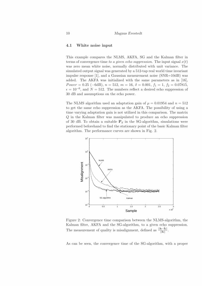
This example compares the NLMS, AKFA, SG and the Kalman filter interms of convergence time to a given echo suppression. The input signal x(t)was zero mean white noise, normally distributed with unit variance. Thesimulated output signal was generated by a 512-tap real world time invariantimpulse response [1], and a Gaussian measurement noise (SNR=10dB) wasadded. The AKFA was initialized with the same parameters as in [16],Power = 0.25 (−6dB), n = 512, m = 16, δ = 0.001, f1 = 1, f2 = 0.07815,ǫ = 10−6, and N = 512. The numbers reflect a desired echo suppression of30 dB and assumptions on the echo power.
The NLMS algorithm used an adaptation gain of µ = 0.01954 and n = 512to get the same echo suppression as the AKFA. The possibility of using atime varying adaptation gain is not utilized in this comparison. The matrixQ in the Kalman filter was manipulated to produce an echo suppressionof 30 dB. To obtain a suitable Pd in the SG-algorithm, simulations wereperformed beforehand to find the stationary point of the basic Kalman filteralgorithm. The performance curves are shown in Fig. 2.
0 0.5 1 1.5 2 2.5 3
x 105
10−4
10−3
10−2
10−1
100
101
Sample
Mis
alig
nmen
t NLMS
AKFA
SG algorithm Kalman
Figure 2: Convergence time comparison between the NLMS-algorithm, theKalman filter, AKFA and the SG-algorithm, to a given echo suppression.
The measurement of quality is misalignment, defined as ||h−h||||h|| .
As can be seen, the convergence time of the SG-algorithm, with a proper
Paper II: Simulations 11
choice of Pd, is similar to that of the Kalman filter. The convergence timeof the AKFA is, as expected, somewhere between that of the NLMS and theKalman filter while its transient response is of the same character as thatof the SG-algorithm and the Kalman filter.
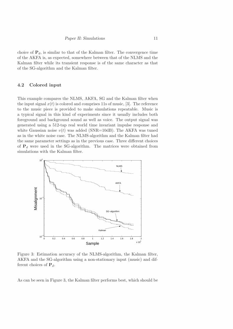
4.2 Colored input
This example compares the NLMS, AKFA, SG and the Kalman filter whenthe input signal x(t) is colored and comprises 11s of music, [3]. The referenceto the music piece is provided to make simulations repeatable. Music isa typical signal in this kind of experiments since it usually includes bothforeground and background sound as well as voice. The output signal wasgenerated using a 512-tap real world time invariant impulse response andwhite Gaussian noise v(t) was added (SNR=10dB). The AKFA was tunedas in the white noise case. The NLMS-algorithm and the Kalman filter hadthe same parameter settings as in the previous case. Three different choicesof Pd were used in the SG-algorithm. The matrices were obtained fromsimulations with the Kalman filter.
0 0.2 0.4 0.6 0.8 1 1.2 1.4 1.6 1.8 2
x 105
10−2
10−1
100
Sample
Mis
alig
nmen
t
AKFA
NLMS
SG−algorithm
Kalman
Figure 3: Estimation accuracy of the NLMS-algorithm, the Kalman filter,AKFA and the SG-algorithm using a non-stationary input (music) and dif-ferent choices of Pd.
As can be seen in Figure 3, the Kalman filter performs best, which should be

12 Magnus Evestedt
expected considering the colored input. The AKFA performs significantlybetter than the NLMS algorithm. The SG algorithm performs similarly tothe Kalman filter for the different choices of Pd.
4.3 Piecewise stationary input
This example provides some insight into the importance of the choice ofPd. The input signal toggled between two zero mean, white noise processes,e1(t) and e2(t) with different variances, σ1 and σ2,
The output signal was generated as in the colored input example, with atruncated impulse response of 64 taps. The Pd-matrix was selected as thestationary solution to the Riccati equation, obtained by simulation, with thecorresponding input signal.
Two simulations were performed. The first one compares the Kalman filterwith the SG algorithm, when it is known beforehand when the input signalshifts. At each such shift Pd is also changed accordingly. The results areshown in Fig. 4. As can be seen the performance of the two algorithms
0 0.5 1 1.5 2 2.5 3
x 105
10−5
10−4
10−3
10−2
10−1
100
101
Sample
Mis
alig
nmen
t
SG−algorithm Kalman
Figure 4: Estimation accuracy of the SG algorithm and the Kalman fil-ter using a piecewise stationary input with scheduled Pd. The curves arevirtually indistinguishable.

Paper II: Simulations 13
is almost identical in this case. If Pd is instead set constant, the resultsobtained are shown in Fig. 5.
0 0.5 1 1.5 2 2.5 3
x 105
10−5
10−4
10−3
10−2
10−1
100
101
Sample
Mis
alig
nmen
t
SG−algorithm
Kalman
Figure 5: Estimation accuracy of the SG algorithm and the Kalman filterusing a piecewise stationary input with constant Pd
Figures 4 and 5 indicate that the choice of Pd in the SG algorithm is im-portant to the estimation performance. If it is known that the input signalwill be piecewise stationary, solving the algebraic Riccati equation for eachperiod of stationarity gives the best choice of Pd at each stationarity interval.
4.4 Input signal with decreasing energy
In this example, the same 11s of music as in the case of colored input wereused as input signal. The energy in the signal was however decreased overtime to study the algorithms’ robustness to windup. During the first secondsof the experiment, the input signal was white noise with unit variance toprovide the algorithms with sufficient initial excitation. The output wascreated using a 512 tap impulse response.
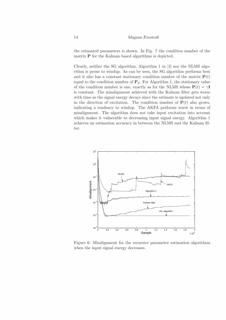
The goal with this setup was to compare how the NLMS, the AKFA, theSG algorithm, the Kalman filter and the method referred to as Algorithm1 in [4], react to partial loss of excitation. In Fig. 6 the misalignment of
14 Magnus Evestedt
the estimated parameters is shown. In Fig. 7 the condition number of thematrix P for the Kalman based algorithms is depicted.
Clearly, neither the SG algorithm, Algorithm 1 in [4] nor the NLMS algo-rithm is prone to windup. As can be seen, the SG algorithm performs bestand it also has a constant stationary condition number of the matrix P(t)equal to the condition number of Pd. For Algorithm 1, the stationary valueof the condition number is one, exactly as for the NLMS whose P(t) = γI
is constant. The misalignment achieved with the Kalman filter gets worsewith time as the signal energy decays since the estimate is updated not onlyin the direction of excitation. The condition number of P(t) also grows,indicating a tendency to windup. The AKFA performs worst in terms ofmisalignment. The algorithm does not take input excitation into accountwhich makes it vulnerable to decreasing input signal energy. Algorithm 1achieves an estimation accuracy in between the NLMS and the Kalman fil-ter.
0 0.2 0.4 0.6 0.8 1 1.2 1.4 1.6 1.8 2
x 105
10−5
10−4
10−3
10−2
10−1
100
101
Sample
Mis
alig
nmen
t
SG−algorithm
Kalman filter
Algorithm 1
AKFA
NLMS
Figure 6: Misalignment for the recursive parameter estimation algorithmswhen the input signal energy decreases.

Paper II: Simulations 15
0 2 4 6 8 10 12 14 16 18
x 104
0
5
10
15
20
25
30
Sample
Con
ditio
n nu
mbe
r
Kalman filter
SG−algorithm
Algorithm 1
Figure 7: The condition number of P(t) for the Kalman filter based recursiveparameter estimation algorithms when the input signal energy decreases.Condition number for the NLMS algorithm is always one.
4.5 Tracking
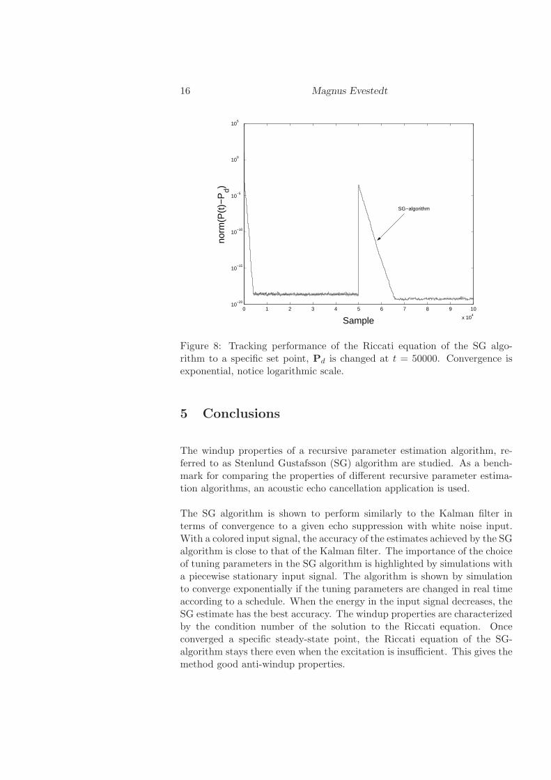
In this example the tracking performance of the SG algorithm is studied.The input signal was zero mean white noise with variance σ = 5. The outputsignal was created using a 64 tap impulse response. If Pd is considered asa reference signal to the SG algorithm, the tracking time is defined as thetime for the algorithm to converge to a specific Pd. Here it is illustrated bysimulating a change of Pd at time t = 50000. The results are shown in Fig.8. As can be seen in the figure, the algorithm converges exponentially, asthe Kalman filter [7].
When the excitation is nonpersistent, there is a manifold of stationary so-lutions to the Riccati equation of the SG algorithm (7), [5, 6]. To illustratethis, the input signal was chosen as a constant during the first 50000 sam-ples. Fig. 9 shows the simulation results. When the input signal is notpersistently exciting, the difference between the stationary solution and Pd
is constant. When the excitation is recovered, the solution however con-verges to the matrix Pd.
16 Magnus Evestedt
0 1 2 3 4 5 6 7 8 9 10
x 104
10−20
10−15
10−10
10−5
100
105
Sample
norm
(P(t
)−P
d)SG−algorithm
Figure 8: Tracking performance of the Riccati equation of the SG algo-rithm to a specific set point, Pd is changed at t = 50000. Convergence isexponential, notice logarithmic scale.
5 Conclusions
The windup properties of a recursive parameter estimation algorithm, re-ferred to as Stenlund Gustafsson (SG) algorithm are studied. As a bench-mark for comparing the properties of different recursive parameter estima-tion algorithms, an acoustic echo cancellation application is used.
The SG algorithm is shown to perform similarly to the Kalman filter interms of convergence to a given echo suppression with white noise input.With a colored input signal, the accuracy of the estimates achieved by the SGalgorithm is close to that of the Kalman filter. The importance of the choiceof tuning parameters in the SG algorithm is highlighted by simulations witha piecewise stationary input signal. The algorithm is shown by simulationto converge exponentially if the tuning parameters are changed in real timeaccording to a schedule. When the energy in the input signal decreases, theSG estimate has the best accuracy. The windup properties are characterizedby the condition number of the solution to the Riccati equation. Onceconverged a specific steady-state point, the Riccati equation of the SG-algorithm stays there even when the excitation is insufficient. This gives themethod good anti-windup properties.
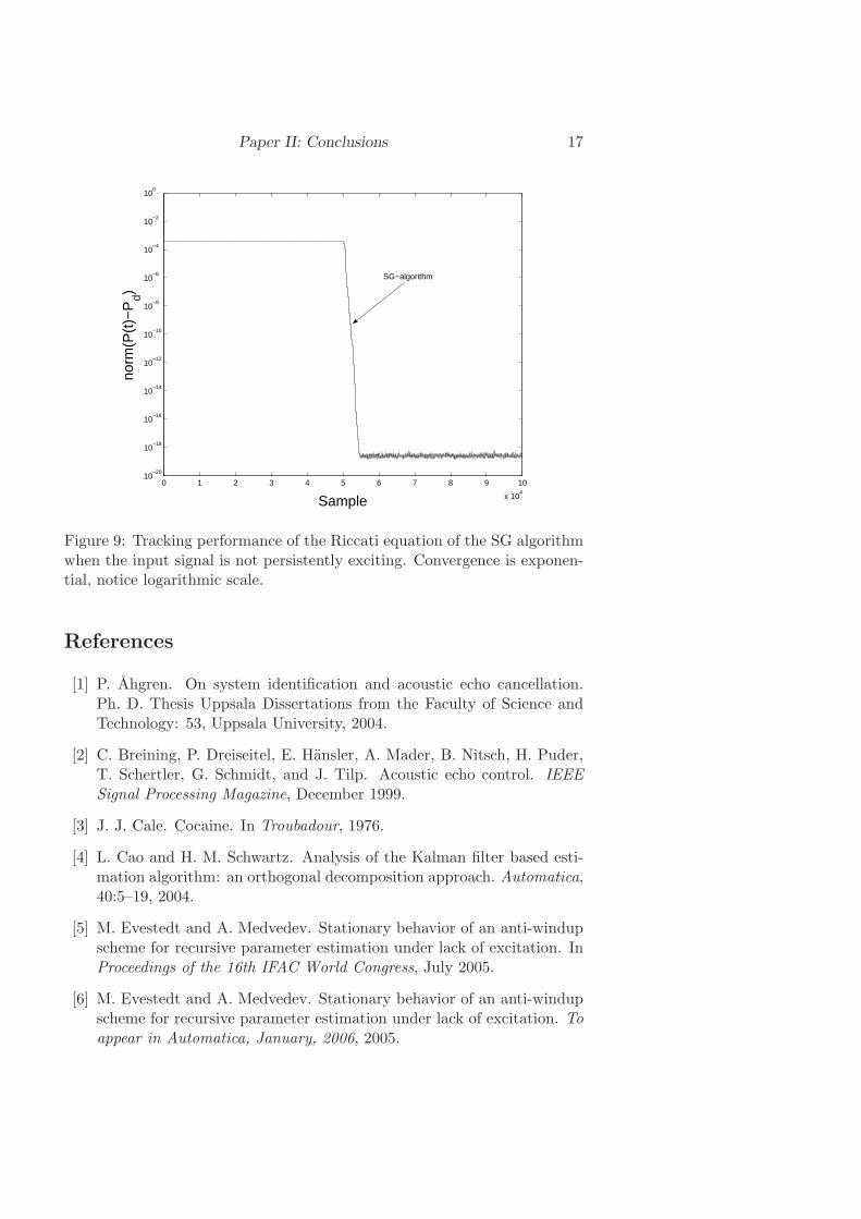
Paper II: Conclusions 17
0 1 2 3 4 5 6 7 8 9 10
x 104
10−20
10−18
10−16
10−14
10−12
10−10
10−8
10−6
10−4
10−2
100
Sample
norm
(P(t
)−P
d)
SG−algorithm
Figure 9: Tracking performance of the Riccati equation of the SG algorithmwhen the input signal is not persistently exciting. Convergence is exponen-tial, notice logarithmic scale.
References
[1] P. Ahgren. On system identification and acoustic echo cancellation.Ph. D. Thesis Uppsala Dissertations from the Faculty of Science andTechnology: 53, Uppsala University, 2004.
[2] C. Breining, P. Dreiseitel, E. Hansler, A. Mader, B. Nitsch, H. Puder,T. Schertler, G. Schmidt, and J. Tilp. Acoustic echo control. IEEESignal Processing Magazine, December 1999.
[3] J. J. Cale. Cocaine. In Troubadour, 1976.
[4] L. Cao and H. M. Schwartz. Analysis of the Kalman filter based esti-mation algorithm: an orthogonal decomposition approach. Automatica,40:5–19, 2004.
[5] M. Evestedt and A. Medvedev. Stationary behavior of an anti-windupscheme for recursive parameter estimation under lack of excitation. InProceedings of the 16th IFAC World Congress, July 2005.
[6] M. Evestedt and A. Medvedev. Stationary behavior of an anti-windupscheme for recursive parameter estimation under lack of excitation. Toappear in Automatica, January, 2006, 2005.
18 Magnus Evestedt
[7] G. C. Goodwin and K. S. Sin. Adaptive filtering prediction and control.Englewood Cliffs: Prentice-Hall, 1984.
[8] S. Gunnarsson. Combining tracking and regularization in recursive leastsquares identification. In Proceedings of the 35th IEEE Conference onDecision and Control, pages 2551–2552, 1996.
[9] E. Hansler. The hands-free telephone problem-an annotated bibliogra-phy. Signal Processing, 27(3):259–271, 1992.
[10] A. H. Jazwinski. Stochastic processes and filtering theory. AcademicPress, New York, 1970.
[11] A. P. Liavas and P. A. Regalia. Acoustic echo cancellation: do IIRmodels offer better modelling capabilities than their FIR counterparts?IEEE transactions on signal processing, 46(9), September 1998.
[12] L. Ljung and S. Gunnarsson. Adaptation and tracking in system iden-tification - a survey. Automatica, 26(1):7–21, 1990.
[13] A. Medvedev. Stability of a Riccati equation arising in recursive pa-rameter estimation under lack of excitation. IEEE Transactions onAutomatic Control, 49(12):2275–2280, December 2004.
[14] L. S. H. Ngia. Recursive identification of acoustic echo systems usingorthonormal basis functions. IEEE transactions on speech and audioprocessing, 11(3), May 2003.
[15] B. Stenlund and F. Gustafsson. Avoiding windup in recursive parameterestimation. In Preprints of reglermote 2002, Linkoping, Sweden, May2002.
[16] T. Wigren. Fast converging and low complexity adaptive filtering usingan averaged Kalman filter. IEEE Transactions on Signal Processing,46(2):515–518, February 1998.

Paper III


Gas jet impinging on liquid surface: Cavity
spaciotemporal modelling and estimation
Magnus Evestedt and Alexander Medvedev
Abstract
A water model is studied to simulate physical phenomena in the LDsteel converter. The depression in the liquid, due to the impinging gasjet, is measured by means of a video camera. Image processing toolstogether with a nonlinear mathematical model based on the physicsof the liquid-gas system, are used to describe the cavity profile. Themodel is shown to give rise to periodic spatial solutions of the liquiddepression for large radial distances from the origin. Under the as-sumption that the cavity profile is stationary, a quantification of theuncertainty of the depth and diameter estimates is given. The varianceof the estimates is shown, by experiments, to decrease by 50% underthe assumption that the the cavity depth and diameter oscillations canbe described as a sum of a small number of sine waves.
1 Introduction
A jet of gas impinging on the surface of a liquid has many industrial ap-plications. The focus of this paper is on modelling a steel making processinvolving top blowing e. g. the LD converter. It is widely used and standsfor approximately 60% of the total world steel production , [18].
The main principle of the LD process is to reduce, by oxidization, the con-tents of carbon, silicon and other contaminating components in the moltenmetal. In the LD converter, oxygen is jetted onto the liquid iron surfacefrom the top, through a lance, at supersonic speed. In the interaction area
1
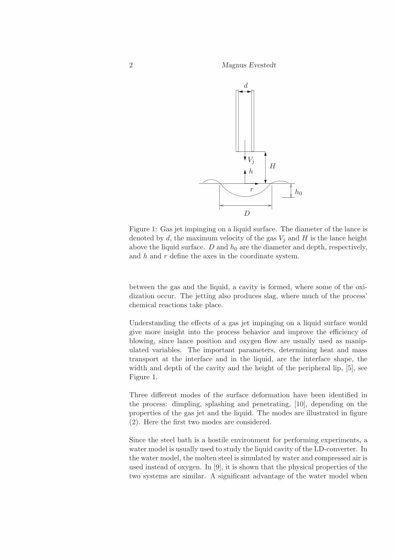
2 Magnus Evestedt
d
Vj
h
r
H
D
h0
Figure 1: Gas jet impinging on a liquid surface. The diameter of the lance isdenoted by d, the maximum velocity of the gas Vj and H is the lance heightabove the liquid surface. D and h0 are the diameter and depth, respectively,and h and r define the axes in the coordinate system.
between the gas and the liquid, a cavity is formed, where some of the oxi-dization occur. The jetting also produces slag, where much of the process’chemical reactions take place.
Understanding the effects of a gas jet impinging on a liquid surface wouldgive more insight into the process behavior and improve the efficiency ofblowing, since lance position and oxygen flow are usually used as manip-ulated variables. The important parameters, determining heat and masstransport at the interface and in the liquid, are the interface shape, thewidth and depth of the cavity and the height of the peripheral lip, [5], seeFigure 1.
Three different modes of the surface deformation have been identified inthe process: dimpling, splashing and penetrating, [10], depending on theproperties of the gas jet and the liquid. The modes are illustrated in figure(2). Here the first two modes are considered.
Since the steel bath is a hostile environment for performing experiments, awater model is usually used to study the liquid cavity of the LD-converter. Inthe water model, the molten steel is simulated by water and compressed air isused instead of oxygen. In [9], it is shown that the physical properties of thetwo systems are similar. A significant advantage of the water model when
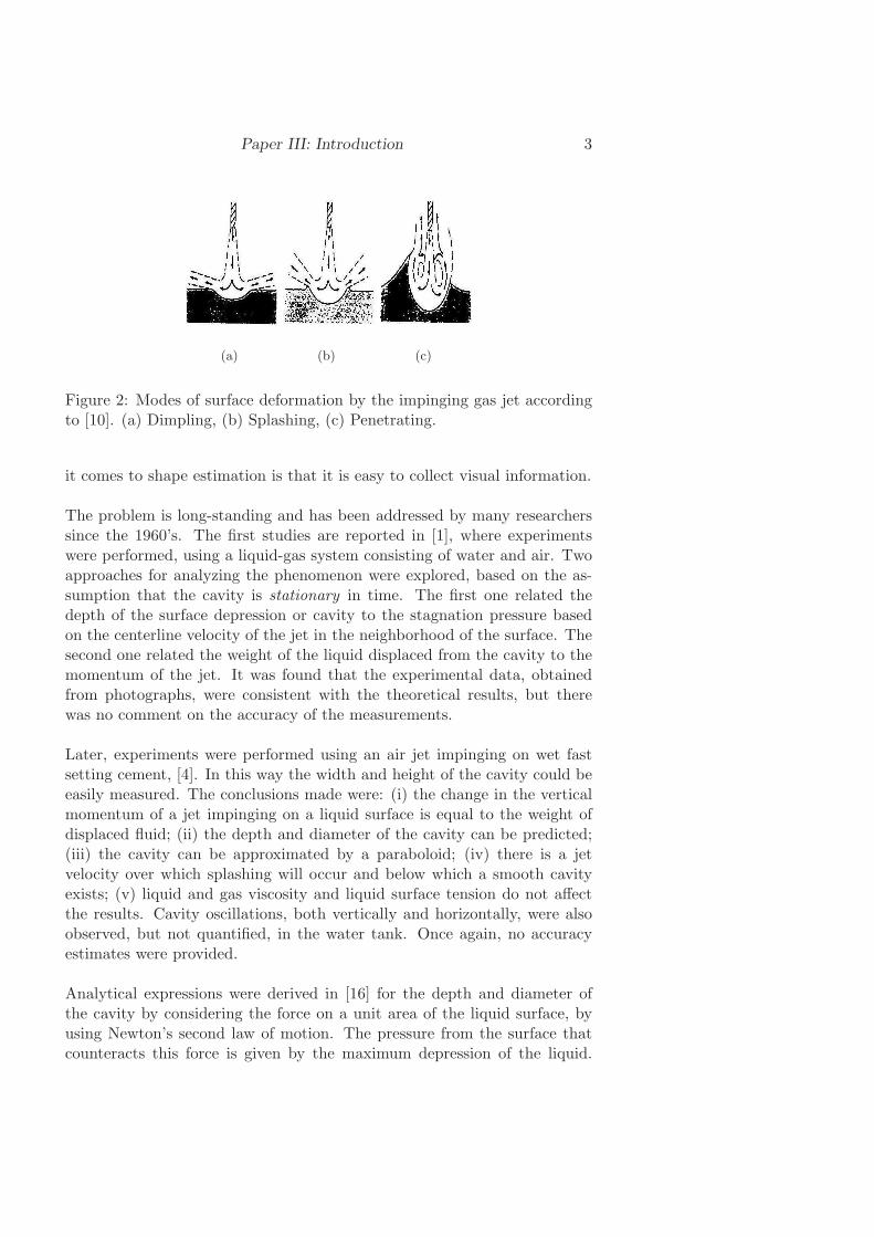
Paper III: Introduction 3
(a) (b) (c)
Figure 2: Modes of surface deformation by the impinging gas jet accordingto [10]. (a) Dimpling, (b) Splashing, (c) Penetrating.
it comes to shape estimation is that it is easy to collect visual information.
The problem is long-standing and has been addressed by many researcherssince the 1960’s. The first studies are reported in [1], where experimentswere performed, using a liquid-gas system consisting of water and air. Twoapproaches for analyzing the phenomenon were explored, based on the as-sumption that the cavity is stationary in time. The first one related thedepth of the surface depression or cavity to the stagnation pressure basedon the centerline velocity of the jet in the neighborhood of the surface. Thesecond one related the weight of the liquid displaced from the cavity to themomentum of the jet. It was found that the experimental data, obtainedfrom photographs, were consistent with the theoretical results, but therewas no comment on the accuracy of the measurements.
Later, experiments were performed using an air jet impinging on wet fastsetting cement, [4]. In this way the width and height of the cavity could beeasily measured. The conclusions made were: (i) the change in the verticalmomentum of a jet impinging on a liquid surface is equal to the weight ofdisplaced fluid; (ii) the depth and diameter of the cavity can be predicted;(iii) the cavity can be approximated by a paraboloid; (iv) there is a jetvelocity over which splashing will occur and below which a smooth cavityexists; (v) liquid and gas viscosity and liquid surface tension do not affectthe results. Cavity oscillations, both vertically and horizontally, were alsoobserved, but not quantified, in the water tank. Once again, no accuracyestimates were provided.
Analytical expressions were derived in [16] for the depth and diameter ofthe cavity by considering the force on a unit area of the liquid surface, byusing Newton’s second law of motion. The pressure from the surface thatcounteracts this force is given by the maximum depression of the liquid.
4 Magnus Evestedt
The predictions were validated on a system with different liquids and argonor nitrogen jet streams. The analytical expressions were found to agreewith the experimental results, but the variance of the measurements wasnot given.
In an attempt to predict the whole cavity profile, a nonlinear singular inte-gral equation was formulated in [12], using conformal mapping methods andfinite Hilbert transforms. The results were, however, limited to small angledepressions in the liquid surface. Later, new numerical procedures were de-veloped, that allowed the depressions to be slightly deeper, [17]. The modelwas found to be consistent with the experimental data reported in [1], butonly for large lance heights.
Energy and force balances were analyzed in [14], to describe the indentationprofile. The calculated profile was found to agree with a cavity profile ob-tained in experiments, but the quality of the measurements was not given.These results were later used in [2], for a study of the stability of interfacesbetween fluids in motion, special attention being given to the role of surfacetension. It was found that increasing surface tension has a stabilizing effect,while increasing the gas density or jet velocity is destabilizing.
More recently, experiments were carried out using a water-air system, [5].Sophisticated image processing was used to measure the important param-eters describing the cavity. The shape of the cavity was found to be eitherparabolic or Gaussian depending on the conditions of the jet flow and theliquid bath. The results were also compared to those found in [1] and [4].The comparison shows that the estimates in [1] and [4] overestimated thecavity width and height, because the theory did not properly account forthe effects of the liquid viscosity and surface tension. The oscillations of thecavity were neglected in the experiments.
A physical modeling study of the effects of top blowing was performed in[11]. There the effects of nozzle diameter, lance height and flow rate on thepenetration depth were investigated and empirically modelled.
All the work performed previously has been based on the assumption of sta-tionary properties of the cavity. On the other hand, cavity oscillations havebeen observed in the water tank during the experiments that should leadto a large variance in the estimates based on the stationarity assumption.The purpose of this paper is to combine the experimental data obtained byimage processing with a mathematical model of the cavity. The uncertain-ties in the depth and diameter estimates under the stationarity assumptionare quantified using a sequence of images. Furthermore, a mathematicaldescription of the temporal behaviour of the cavity depth and diameter is

Paper III: Mathematical models 5
proposed to decrease the variance of the estimates.
Three following insights motivate the approach to obtain a description ofthe whole cavity, not only the depth and diameter.
• Mathematical models based on approximation techniques lack con-nection to the physics of the process and often lead to inconclusiveresults.
• A mathematical model of the liquid-gas jet system has to be richenough in order to explain the cavity profiles observed in the watermodel.
• Dynamics of the temporal variations in the cavity depth and diameterhave to be taken into account to yield reasonable estimate variance.
The organization of the paper is as follows. First the mathematical modelof the cavity is given and its stability properties are analyzed. Then theexperimental setup is described. The paper is concluded with the results ofdepth and diameter estimation, under the assumption of stationary cavityand oscillating cavity, respectively.
2 Mathematical models
Mathematical modelling of the cavity is important to extract valuable in-formation from the image in the face of disturbance. Due to the difficultiesof estimating the form of the cavity, the researchers have concentrated ona few key parameters such as depth and diameter of the depression. Manysuggestions on the cavity profile, such as paraboloid, ellipsoid or Gaussianform, have been made in the past, [4], [5]. Another equation that describesthe cavity is the inverted hyperbolic cosine function, [6], h(r) = a
cosh2 (b(r−c)),
where a is the amplitude of the function and b is a parameter that affectsthe width. The parameter c allows the cavity to move sideways.
The results of approximation of an experimentally obtained cavity profileby some of those functions are shown in Figure 3. As can be seen, theindentation is described equally well in the cavity itself, but the accuracyof the models differ when larger radial distances from the center are con-sidered. This means that the accuracy of approximation is mainly definedby the spatial interval at which the approximation is considered. Neitherof the models is able to capture the peripheral lips of the cavity. Another
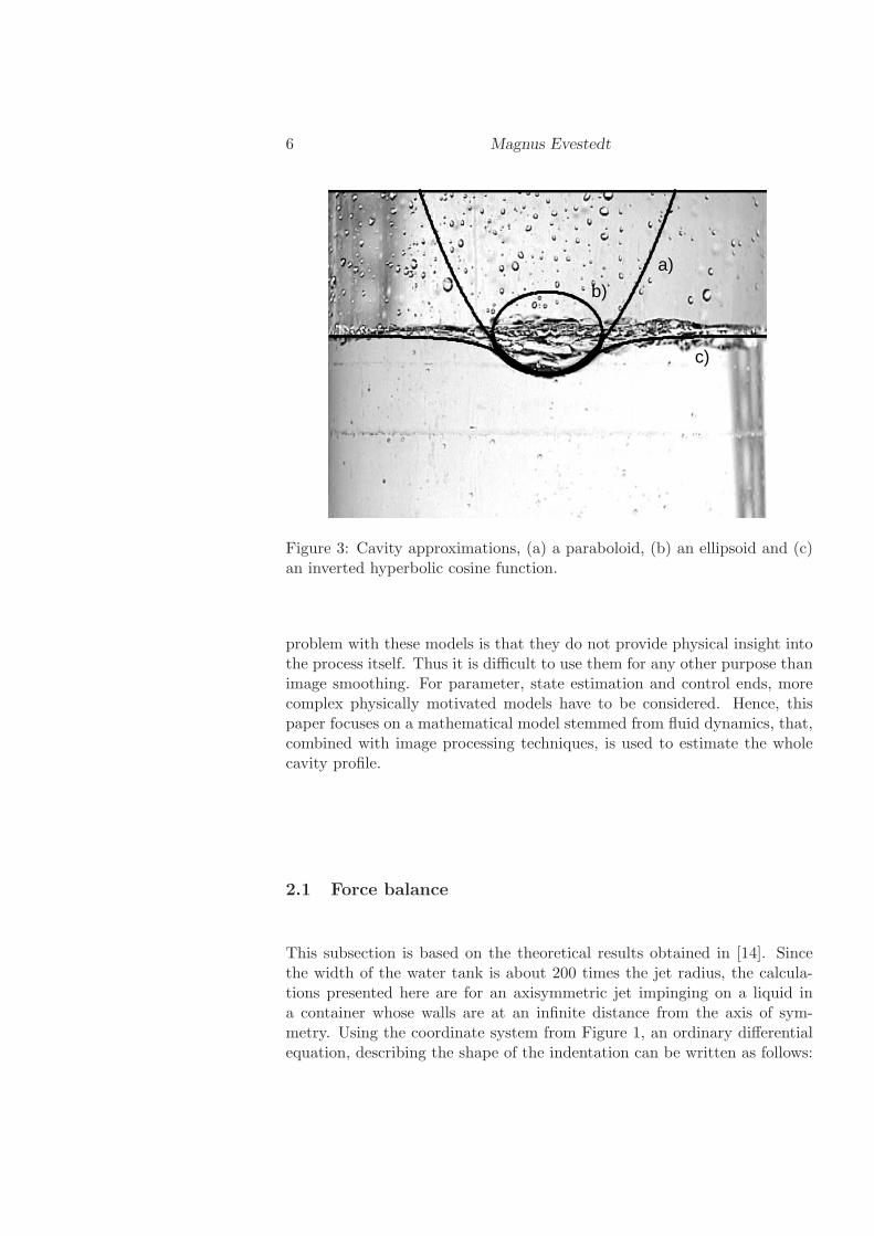
6 Magnus Evestedt
a)
b)
c)
Figure 3: Cavity approximations, (a) a paraboloid, (b) an ellipsoid and (c)an inverted hyperbolic cosine function.
problem with these models is that they do not provide physical insight intothe process itself. Thus it is difficult to use them for any other purpose thanimage smoothing. For parameter, state estimation and control ends, morecomplex physically motivated models have to be considered. Hence, thispaper focuses on a mathematical model stemmed from fluid dynamics, that,combined with image processing techniques, is used to estimate the wholecavity profile.
2.1 Force balance
This subsection is based on the theoretical results obtained in [14]. Sincethe width of the water tank is about 200 times the jet radius, the calcula-tions presented here are for an axisymmetric jet impinging on a liquid ina container whose walls are at an infinite distance from the axis of sym-metry. Using the coordinate system from Figure 1, an ordinary differentialequation, describing the shape of the indentation can be written as follows:
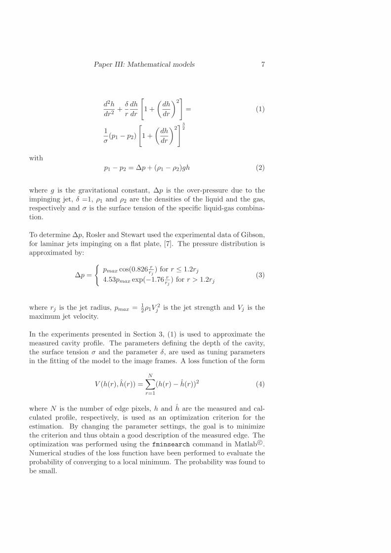
Paper III: Mathematical models 7
d2h
dr2+
δ
r
dh
dr
[
1 +
(dh
dr
)2]
= (1)
1
σ(p1 − p2)
[
1 +
(dh
dr
)2] 3
2
with
p1 − p2 = ∆p + (ρ1 − ρ2)gh (2)
where g is the gravitational constant, ∆p is the over-pressure due to theimpinging jet, δ =1, ρ1 and ρ2 are the densities of the liquid and the gas,respectively and σ is the surface tension of the specific liquid-gas combina-tion.
To determine ∆p, Rosler and Stewart used the experimental data of Gibson,for laminar jets impinging on a flat plate, [7]. The pressure distribution isapproximated by:
∆p =
{
pmax cos(0.826 rrj
) for r ≤ 1.2rj
4.53pmax exp(−1.76 rrj
) for r > 1.2rj(3)
where rj is the jet radius, pmax = 12ρ1V
2j is the jet strength and Vj is the
maximum jet velocity.
In the experiments presented in Section 3, (1) is used to approximate themeasured cavity profile. The parameters defining the depth of the cavity,the surface tension σ and the parameter δ, are used as tuning parametersin the fitting of the model to the image frames. A loss function of the form
V (h(r), h(r)) =N∑
r=1
(h(r) − h(r))2 (4)
where N is the number of edge pixels, h and h are the measured and cal-culated profile, respectively, is used as an optimization criterion for theestimation. By changing the parameter settings, the goal is to minimizethe criterion and thus obtain a good description of the measured edge. Theoptimization was performed using the fminsearch command in Matlab c©.Numerical studies of the loss function have been performed to evaluate theprobability of converging to a local minimum. The probability was found tobe small.

8 Magnus Evestedt
−10
−5
0
5
10
−1
−0.5
0
0.5
10
200
400
600
800
1000
x1
x2
r
Figure 4: Trajectories of the system with different initial values.
2.2 Stability analysis
The system described in (1) can be formulated in state-space form as
dx
dr=
{
x2
1σ (∆p + (ρ1 − ρ2)gx1)
[1 + x2
2
] 32 − δ
rx2
[1 + x2
2
] (5)
x = [x1 x2]T
where x1 = h and x2 = dhdr .
Since r is the integration variable in the state-space formulation and appearsexplicitly in the right-hand side of the equation, using a phase portrait isnot feasible. A three dimensional plot of the evolution of (5) with increasingr, for different initial points, is shown in figure (4).
Taking into account that limr→∞ ∆p = limr→∞δr = 0 the steady-state sys-
tem is
dx
dr=
{
x2
1σ ((ρ1 − ρ2)gx1)
[1 + x2
2
] 32
(6)
The dynamics of (6) give rise to sustained periodic solutions as proven bythe proposition below.

Paper III: Experiments 9
Proposition Consider the function
V (x) =1
(1 + x22)
1/2−
c
2x2
1 (7)
where c = 1σ (ρ2 − ρ1)g, c > 0. Define a set M as the region
M ={x ∈ R
2|c1 ≤ V (x) ≤ c2
}, where 0 < c1 < c2 < 1. Then there is a
periodic solution of (6) in M .
Proof : Consider the system given by (6) and the function (7). The derivativeof V (x) along the trajectories of the system is given by
V (x) = −cx1x1 − x2(1 + x22)
−3/2x2 = 0 (8)
Define a set M as the region
M ={x ∈ R
2|c1 ≤ V (x) ≤ c2
}(9)
where 0 < c1 < c2 < 1. Clearly M is bounded and positively invariant. It isalso free of equilibrium points, since the only equilibrium point of the systemis at the origin. Thus it follows from the Poincare-Bendixson theorem, [8],that there is a periodic solution of (6) in M . �
According to the theoretical results, sustained spatial oscillations arise faraway from the origin, due to the model properties. In the experiments thatfollow in the next section, the water is contained in a tank of finite diameter.
3 Experiments
The experiments were conducted on a water model of the LD converter,previously used to study and control foaming, [3]. A single hole cylindricalnozzle with diameter 1.5 mm is used. The indentation profile arising whenair is jetted onto the liquid surface is recorded using a CCD camera.
3.1 Video measurement
A digital video camera captures the cavity during the blow. The shoot angleof the camera can be easily changed. In these experiments the tank is filmeddirectly from the side of the water tank, creating a two-dimensional image.Since the jet-forming nozzle on the lance providing the gas is symmetric,the depression should be rotation symmetric. The video camera produces asequence of image frames that is the information source in the estimation ofthe cavity shape and can as well be used to discern its temporal pattern.

10 Magnus Evestedt
3.1.1 Camera calibration
The frames collected from the video camera are represented by pixel val-ues. It is desirable to express the axis of the images in length units andthus a conversion between them is performed. Special care is also taken tocompensate for a tilted image, due to the camera setting.
3.1.2 Light settings
In photography, the lighting has to be designed beforehand to obtain the bestimaging results. This is especially important for image processing purposes.The lighting has to suit the camera and the purpose of filming or else theimage can be useless. Incorrect light settings result in shadows, glares andunwanted reflections in the water surface. In these experiments the watertank was lit from the side with a reflector behind, which is proven to providethe best lighting conditions.
3.2 Image processing
To extract the edges from the image an in-house software is used. Theframes of the video sequence are filtered to reduce the noise in the image.Then edge detection is applied using a thresholding method, together withsome basic image processing tools such as opening, closing and flood-fill,[15].
3.3 Sources of error
There are several sources of error in the experimental setup.
• The oxygen flow through the lance is slowly varying with time.
• The lance angle to the water bath cannot be guaranteed to be 90degrees at all heights.
• Bubbles and splashing make the edge detection difficult.

Paper III: Results 11
10 11 12 13 14 15 16 17 18 19 2017
18
19
20
21
22
23
24
25
26
27
Lance height [cm]
Gas
flow
rat
e [l/
min
]
1 2 3
4 5 6
7 8 9
10 11 12
Figure 5: The studied settings of lance height and gas flow rates used in 12experiments with the water model. Each triangle corresponds to a specificexperiment.
4 Results
In this section the results obtained from water model experiments are sum-marized. First edge detection in the video frames is discussed. Then thecavity depth and diameter are estimated using the assumption that they areconstant for each setting of experimental conditions. The variance of theobtained estimates is compared to that of the estimates obtained under theassumption that the depth and diameter are changing with time.
Twelve different settings of gas flow rate and lance height were studied andare illustrated in Figure 5. The values are selected so that a well-definedcavity can be seen in the water tank.
4.1 Image processing results
The cavity shape measurements are given in the form of images obtainedby a video camera. To be able to compare the image to a mathematicalfunction, the edge of the cavity is extracted from the measurement. The
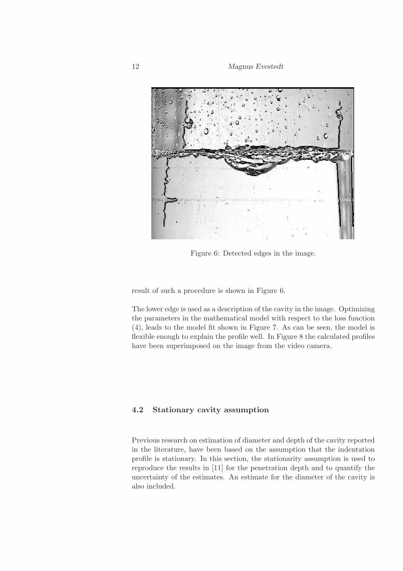
12 Magnus Evestedt
Figure 6: Detected edges in the image.
result of such a procedure is shown in Figure 6.
The lower edge is used as a description of the cavity in the image. Optimizingthe parameters in the mathematical model with respect to the loss function(4), leads to the model fit shown in Figure 7. As can be seen, the model isflexible enough to explain the profile well. In Figure 8 the calculated profileshave been superimposed on the image from the video camera.
4.2 Stationary cavity assumption
Previous research on estimation of diameter and depth of the cavity reportedin the literature, have been based on the assumption that the indentationprofile is stationary. In this section, the stationarity assumption is used toreproduce the results in [11] for the penetration depth and to quantify theuncertainty of the estimates. An estimate for the diameter of the cavity isalso included.

Paper III: Results 13
0 0.5 1 1.5 2 2.5 3 3.5 4 4.5 5
−0.8
−0.7
−0.6
−0.5
−0.4
−0.3
−0.2
−0.1
0
Radial distance [cm]
Dep
ress
ion
[cm
]
ApproximationCavity edge
Figure 7: Approximation of the cavity profile using a mathematical modelbased on force balance. The approximated cavity is shown together withthe measured edge.
Figure 8: Approximation of the cavity profile for a mathematical modelbased on force balance. The approximated cavity is superimposed on animage frame.
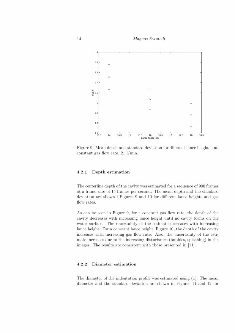
14 Magnus Evestedt
13.5 14 14.5 15 15.5 16 16.5 17 17.5 18 18.52.4
2.6
2.8
3
3.2
3.4
3.6
3.8
4
Dep
th
Lance height [cm]
Figure 9: Mean depth and standard deviation for different lance heights andconstant gas flow rate, 21 l/min.
4.2.1 Depth estimation
The centerline depth of the cavity was estimated for a sequence of 900 framesat a frame rate of 15 frames per second. The mean depth and the standarddeviation are shown i Figures 9 and 10 for different lance heights and gasflow rates.
As can be seen in Figure 9, for a constant gas flow rate, the depth of thecavity decreases with increasing lance height until no cavity forms on thewater surface. The uncertainty of the estimate decreases with increasinglance height. For a constant lance height, Figure 10, the depth of the cavityincreases with increasing gas flow rate. Also, the uncertainty of the esti-mate increases due to the increasing disturbance (bubbles, splashing) in theimages. The results are consistent with those presented in [11].
4.2.2 Diameter estimation
The diameter of the indentation profile was estimated using (1). The meandiameter and the standard deviation are shown in Figures 11 and 12 for

Paper III: Results 15
18 19 20 21 22 23 24 25 262
2.5
3
3.5
Dep
th
Flow [l/min]
Figure 10: Mean depth and standard deviation for different gas flow ratesand constant lance height, 14 cm.
different lance heights and gas flow rates.
The large standard deviations in Figures 11 and 12 indicate that the diam-eter of the cavity is more volatile than the depth. It also shows that theassumption of a stationary cavity fails to provide consistent estimates.
4.3 Dynamic cavity assumption
The estimates of the cavity depth and diameter are, in each image frame,obtained from the model. Since the force balance model does not account forthe temporal cavity oscillation, the assumption that the process is stationaryleads to an unnecessarily large variance of the estimates.
Here the assumption that the cavity oscillations, both in diameter and depth,are periodic is investigated. A natural base function for describing such asignal is the sine wave. The proposed model is a sum of a number of sine

16 Magnus Evestedt
11.5 12 12.5 13 13.5 14 14.5 15 15.5 16 16.54
5
6
7
8
9
10
Dia
met
er
Lance height [cm]
Figure 11: Mean diameter and standard deviation for different lance heightsand constant gas flow rate, 21 l/min.
18 19 20 21 22 23 24 25 264
5
6
7
8
9
10
11
12
13
14
Dia
met
er
Flow [l/min]
Figure 12: Mean diameter and standard deviation for different gas flow ratesand constant lance height, 14 cm.

Paper III: Results 17
waves
h0 =n∑
i=1
Ah0(i) sin(ωh0(i)t + φh0(i)) (10)
D =n∑
i=1
AD(i) sin(ωD(i)t + φD(i))
where n is a small integer. The parameters Ah0(i), AD(i), ωh0(i), ωD(i),φh0(i) and φD(i) are estimated using the estimated depth and diametersequences, respectively. The most prominent frequency is estimated usingthe Quinn and Fernandes technique, [13], and removed from the signal us-ing regression. The residual is used to estimate the next frequency, etc.Finally the estimated frequencies are used simultaneously to estimate theamplitudes and phases.
4.3.1 Depth estimation
Due to the numerous sources of errors, the statistical properties of the depthand diameter estimates are changing. The frequency of the oscillations fluc-tuates during the blow. To cope with this problem, a sliding window of40 frames was used over 300 frames to estimate the time varying sine waveparameters. The windowing results in 260 estimates of the frequencies. Thedrawback of this procedure is that the accuracy of the frequency estimatesis decreased, in favor of better tracking capabilities.
The distribution of the frequency estimates for the first three dominatingfrequencies is shown in Figure 13.
As can be seen in Figure 13, the main frequency content is from 5−6 Hz forthe most prominent estimated frequency. A large part of the energy in thesignal is still in the same interval for the second frequency. For the third,however, the frequency content is spread over the studied frequency interval.This means that the remaining residual after subtracting two sine waves, isnot covered by the model (10).
In Figure 14 the decrease in variance of the estimate for the depth obtainedwith the dynamic assumption is shown as a percentage of the variance of theestimates obtained with the stationary assumption. If one sine wave is usedto describe the depth oscillations, the decrease of variance is above 20% andby using a sum of three sine waves the variance of the depth estimate canbe decreased by more than 50%.

18 Magnus Evestedt
0 1 2 3 4 5 6 7 80
20
40
60
Frequency [Hz]
# of
inst
ance
s
0 1 2 3 4 5 6 7 80
20
40
60
Frequency [Hz]
# of
inst
ance
s
0 1 2 3 4 5 6 7 80
20
40
60
# of
inst
ance
s
Frequency [Hz]
First dominant tone
Second dominant tone
Third dominant tone
Figure 13: The distribution of the frequency estimates for the first,fromtop down, three dominating frequencies in the depth estimate. Each barrepresents how often a certain frequency value is yielded in the estimates.The lance height is 12 cm and the gas flow rate is 21 l/min.
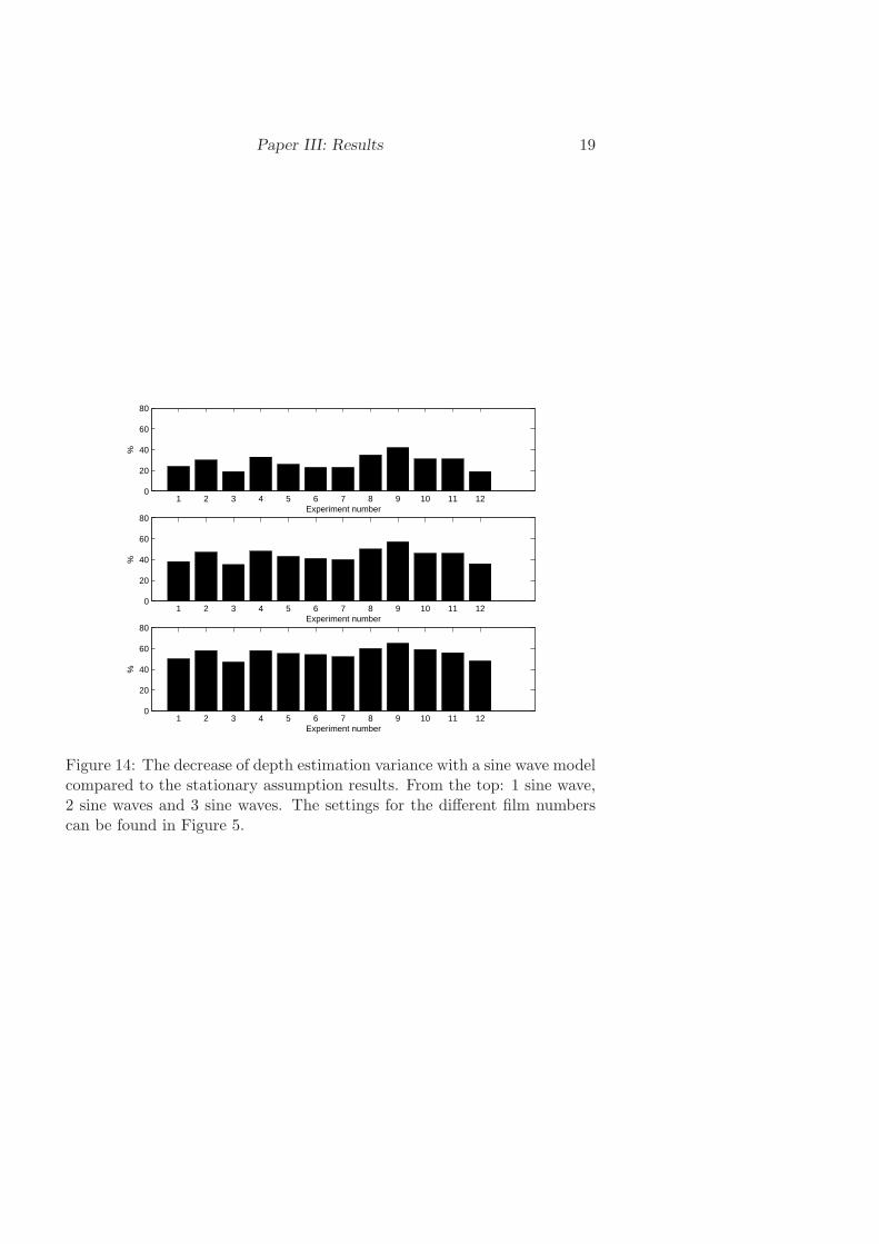
Paper III: Results 19
1 2 3 4 5 6 7 8 9 10 11 120
20
40
60
80
%
Experiment number
1 2 3 4 5 6 7 8 9 10 11 120
20
40
60
80
%
Experiment number
1 2 3 4 5 6 7 8 9 10 11 120
20
40
60
80
%
Experiment number
Figure 14: The decrease of depth estimation variance with a sine wave modelcompared to the stationary assumption results. From the top: 1 sine wave,2 sine waves and 3 sine waves. The settings for the different film numberscan be found in Figure 5.

20 Magnus Evestedt
4.3.2 Diameter estimation
The diameter estimates were treated in the same way as the depth estimates.The frequency content of the windowed measurements is shown in Figure15. It can be seen that the main frequency content lies just above 2 Hz.Estimating the third tone shows that the frequency content is spread overthe studied frequency interval, indicating that the model (10), cannot beused to obtain more information about the oscillations.
0 1 2 3 4 5 6 7 80
50
100
Frequency [Hz]
# of
inst
ance
s
0 1 2 3 4 5 6 7 80
50
100
Frequency [Hz]
# of
inst
ance
s
0 1 2 3 4 5 6 7 80
50
100
Frequency [Hz]
# of
inst
ance
s
First dominant tone
Second dominant tone
Third dominant tone
Figure 15: The distribution of the frequency estimates for the first threedominating frequencies in the diameter estimate. Each bar represents howoften a certain frequency value is yielded in the estimate. The lance heightis 12 cm and the gas flow rate is 21 l/min.
In Figure 16, the accuracy of the diameter estimate based on the stationar-ity assumption is compared to that of the estimate based on the dynamicassumption. It can be seen that by modelling the diameter changes withone sine wave, the variance of the diameter estimate can be decreased bymore than 20% and with three sine waves the decrease is above 50%. Forexperiment number 2 even one sine wave alone reduces the variance of theestimates by 50%. One possible explanation is that for those specific settingsof lance height and gas flow rate, the error sources are not as significant asfor the other films.

Paper III: Results 21
1 2 3 4 5 6 7 8 9 10 11 120
20
40
60
80
%
Experiment number
1 2 3 4 5 6 7 8 9 10 11 120
20
40
60
80
%
Experiment number
1 2 3 4 5 6 7 8 9 10 11 120
20
40
60
80
%
Experiment number
Figure 16: The decrease of diameter estimation variance with a sine wavemodel compared to the stationary assumption results. From the top: 1 sinewave, 2 sine waves and 3 sine waves. The settings for the different filmnumbers can be found in Figure 5.

22 Magnus Evestedt
0 50 100 150 200 2500
0.5
1
1.5
2
2.5
3
3.5
4
4.5
5
Frequency estimate
Dia
met
er/D
epth
Figure 17: The ratio between the 260 dominant frequency estimates for thediameter and the height. The lance height is 16 cm and the gas flow rate is21 l/min.
4.3.3 Cavity oscillations
The depth and the diameter of the cavity oscillate at different frequencies.To characterize the oscillations of the whole cavity, the ratio between thedominant frequency estimates for the depth and diameter is presented inFigure 17.
The mean ratio and the standard deviation for the studied settings of lanceheight and gas flow rate are shown in Figure 18. The large standard devi-ation is an effect of the large peaks, visible in Figure 17. The peaks occurfor all considered settings. However, the frequency ratio stays relativelyconstant under significant periods of time.
5 Conclusions
An experimental and theoretical study of blowing in an LD-converter watermodel has been carried out. A video camera is used to measure the inden-tation profile of the cavity during the blow. Image processing tools together
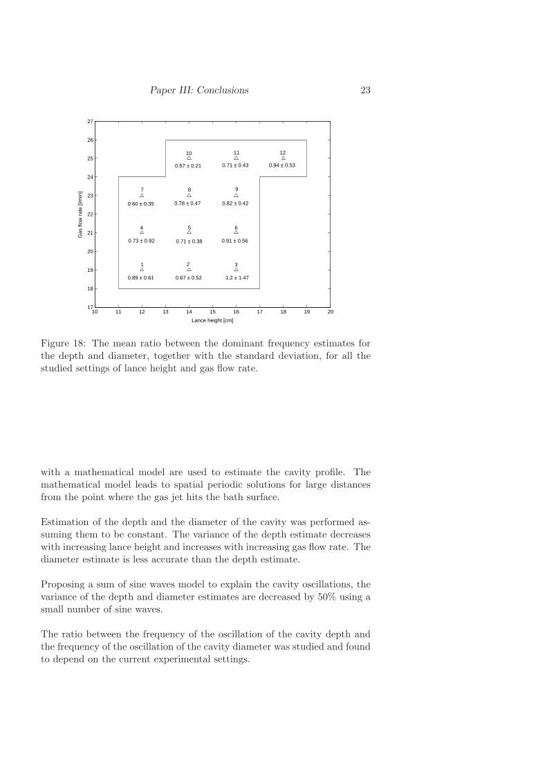
Paper III: Conclusions 23
10 11 12 13 14 15 16 17 18 19 2017
18
19
20
21
22
23
24
25
26
27
Lance height [cm]
Gas
flow
rat
e [l/
min
]
1 2 3
4 5 6
7 8 9
10 11 12
0.89 ± 0.61 0.67 ± 0.52 1.2 ± 1.47
0.73 ± 0.92 0.71 ± 0.38 0.91 ± 0.56
0.60 ± 0.35 0.78 ± 0.47 0.82 ± 0.42
0.57 ± 0.21 0.71 ± 0.43 0.94 ± 0.53
Figure 18: The mean ratio between the dominant frequency estimates forthe depth and diameter, together with the standard deviation, for all thestudied settings of lance height and gas flow rate.
with a mathematical model are used to estimate the cavity profile. Themathematical model leads to spatial periodic solutions for large distancesfrom the point where the gas jet hits the bath surface.
Estimation of the depth and the diameter of the cavity was performed as-suming them to be constant. The variance of the depth estimate decreaseswith increasing lance height and increases with increasing gas flow rate. Thediameter estimate is less accurate than the depth estimate.
Proposing a sum of sine waves model to explain the cavity oscillations, thevariance of the depth and diameter estimates are decreased by 50% using asmall number of sine waves.
The ratio between the frequency of the oscillation of the cavity depth andthe frequency of the oscillation of the cavity diameter was studied and foundto depend on the current experimental settings.
24 Magnus Evestedt
6 Acknowledgments
This work has been in part supported by The Swedish Steel Producers’Association and by the EC 6th Framework programme as a Specific TargetedResearch or Innovation Project (Contract number NMP2-CT-2003-505467).The authors also wish to thank the Department of Process Metallurgy ofthe Royal Institute of Technology, Stockholm, for allowing the authors touse their experimental facilities, Jimmy Tila for help with experiments andsoftware, and Professor Vladimir Pavlenko of Uppsala University for sharinghis vast knowledge of wave theory.
References
[1] R. B. Banks and D. V. Chandrasekhara. Experimental investigationof the penetration of a high-velocity gas jet through a liquid surface.Journal of Fluid Mechanics, 15(103):13–34, 1963.
[2] J. Berghmans. Theoretical investigation of the interfacial stability ofinviscid fluids in motion, considering surface tension. Journal of FluidMechanics, 54:129–141, 1972.
[3] W. Birk, I. Arvanitidis, P. Jonsson, and A. Medvedev. Foam level con-trol in a water model of the LD converter process. Control EngineeringPractice, 11:49–56, 2003.
[4] F. R. Cheslak, J. A. Nicholls, and M. Sichel. Cavities formed on liquidsurfaces by impinging gaseous jets. Journal of Fluid Mechanics, 36:55–64, 1969.
[5] S. Eletribi, D. K. Mukherjee, and V. Prasad. Experiments on liquidsurface deformation upon impingement by a gas jet. In Proceedings ofthe ASME Fluids Engineering Division, volume 244, 1997.
[6] M. Evestedt and A. Medvedev. Cavity depth and diameter estima-tion in the converter process water model,. In Association for Iron& Steel Technology Conference Proceedings, pages 763–771, Nashville,Tennessee, USA, September 2004.
[7] A. H. Gibson. Hydraulics and Its Application. London:Constable, 1934.
[8] H. K. Khalil. Nonlinear systems. Prentice-Hall, Inc, 1996.
[9] M. S. Lee, S. L. O´Rourke, and N. A. Molloy. Fluid flow and surfacewaves in the BOF. ISS Transactions, 29(10):56–65, 2002.

Paper III: Acknowledgments 25
[10] N. A. Molloy. Impinging jet flow in a two-phase system:the basic flowpattern. Journal of the iron and steel institute, pages 943–950, October1970.
[11] A. Nordquist. A physical modeling study of top blowing with focus onthe penetration region. Licentiate thesis, Royal institute of technology,Stockholm, Sweden, 2005.
[12] W. E. Olmstead and S. Raynor. Depression of an infinite liquid surfaceby an incompressible gas jet. Journal of Fluid Mechanics, 19:561–576,1964.
[13] B. G. Quinn and J. M. Fernandes. A fast efficient technique for theestimation of frequency. Biometrika, 78(3):489–497, 1991.
[14] R. S. Rosler and G. H. Stewart. Impingement of gas jets on liquidsurfaces. Journal of Fluid Mechanics, 31:163–174, 1968.
[15] M. Sonka, V. Hlavac, and R. Boyle. Image processing, analysis andmachine vision. PWS Publishing, 1999.
[16] E. T. Turkdogan. Fluid dynamics of gas jets impinging on surface ofliquids. Chemical Engineering Science, 21:1133–1144, 1966.
[17] J. M. Vanden-Broeck. Deformation of a liquid surface by an impinginggas jet. SIAM Journal of Applied Mathematics, 41(2):306–309, 1981.
[18] Steel industry technology roadmap. www.steel.org, June 2005.


Paper IV

Model-based cavity shape estimation in a gas-liquid
system with nonuniform image sampling
Magnus Evestedt and Alexander Medvedev
Abstract
A water model is studied to simulate physical phenomena in theLintz-Donawitz steel converter. The depression in the liquid, due tothe impinging gas jet, is measured by means of a video camera. Imageprocessing tools are used to extract the edge of the surface indentation.The measured edge, sampled in a special way, is used together witha nonlinear mathematical model to obtain a description of the cavityprofile. The parameters of the mathematical model are optimized tomatch the registered cavity edge in the image at a set of sampledpoints. Three ways of choosing sampling points for the optimizationare proposed and compared on simulated as well as experimental data.An approach involving an observer decreases the computation timewith an acceptable loss of accuracy of the estimates.
1 Introduction
The properties of a system consisting of a gas jet impinging on a liquidsurface from above are important in many industrial applications. The focusof this paper is on a steel making process involving top blowing e.g. theLintz-Donawitz (LD) converter. It is widely used and stands for 60% of theworld steel production, [21].
In the LD converter process, hot metal is converted into steel by a top blownbasic oxygen furnace. Scrap and slag forming agents are added to the hotmetal before oxygen is blown onto the metal bath, from above, at supersonic
1

2 Magnus Evestedt
d
Vj
h
r
H
D
h0
Figure 1: Gas jet impinging on a liquid surface. The diameter of the lance isdenoted by d, the maximum velocity of the gas Vj and H is the lance heightabove the liquid surface. D and h0 are the diameter and depth, respectively,and h and r define the axes in the coordinate system.
speed. A cavity is formed where the oxygen jet hits the bath surface andFe, Si, Mn and C are oxidized. The jetting also produces large amounts ofslag, where most of the chemical reactions take place.
The lance position over the bath, together with the oxygen flow rate areusually used as manipulated variables in the process. A deeper understand-ing of the system of the gas jet and the liquid surface would improve theefficiency of blowing and the control of the process. The important parame-ters, determining heat and mass transport at the interface and in the liquid,are the interface shape, the width and depth of the cavity and the height ofthe peripheral lip, [5], see Figure1.
Depending on the properties of the gas jet and the liquid, three modes ofsurface deformation have been identified in the process: dimpling, splashingand penetrating, [9]. The different modes are illustrated in Figure 2. In thispaper only the first two modes are considered.
Since the form of the cavity is difficult to observe in the actual process, dueto the hostile environment, a water model of the LD converter is often used.In the water model the molten steel is replaced by water and compressedair is used instead of oxygen. The similarities between the water bath andthe molten steel are analyzed in [8].

Paper IV: Introduction 3
(a) (b) (c)
Figure 2: Modes of surface deformation by the impinging gas jet accordingto [9]. (a) Dimpling, (b) Splashing, (c) Penetrating.
The problem of modelling the cavity is long-standing and has been addressedby many researchers since the 1960’s. The first studies are reported in [1],where experiments were performed, using a liquid-gas system consisting ofwater and air. Two approaches for analyzing the phenomenon were explored,based on the assumption that the cavity is stationary in time. The firstone related the depth of the surface depression or cavity to the stagnationpressure based on the centerline velocity of the jet in the neighborhood of thesurface. The second one related the weight of the liquid displaced from thecavity to the momentum of the jet. It was found that the experimental data,obtained from photographs, were consistent with the theoretical results, butthere was no comment on the accuracy of the measurements.
Later, experiments were performed using an air jet impinging on wet fastsetting cement, [4]. In this way the width and height of the cavity could beeasily measured. The conclusions made were: (i) the change in the verticalmomentum of a jet impinging on a liquid surface is equal to the weight ofdisplaced fluid; (ii) the depth and diameter of the cavity can be predicted;(iii) the cavity can be approximated by a paraboloid; (iv) there is a jetvelocity over which splashing will occur and below which a smooth cavityexists; (v) liquid and gas viscosity and liquid surface tension do not affectthe results. Cavity oscillations, both vertically and horizontally, were alsoobserved, but not quantified, in the water tank. Once again, no accuracyestimates were provided.
Analytical expressions were derived in [19] for the depth and diameter ofthe cavity by considering the force on a unit area of the liquid surface, byusing Newton’s second law of motion. The pressure from the surface thatcounteracts this force is given by the maximum depression of the liquid.The predictions were validated on a system with different liquids and argonor nitrogen jet streams. The analytical expressions were found to agree

4 Magnus Evestedt
with the experimental results, but the variance of the measurements wasnot given.
In an attempt to predict the whole cavity profile, a nonlinear singular inte-gral equation was formulated in [12], using conformal mapping methods andfinite Hilbert transforms. The results were, however, limited to small angledepressions in the liquid surface. Later, new numerical procedures were de-veloped, that allowed the depressions to be slightly deeper, [20]. The modelwas found to be consistent with the experimental data reported in [1], butonly for large lance heights.
Energy and force balances were analyzed in [14], to describe the indentationprofile. The calculated profile was found to agree with a cavity profile ob-tained in experiments, but the quality of the measurements was not given.These results were later used in [2], for a study of the stability of interfacesbetween fluids in motion, special attention being given to the role of surfacetension. In contrast with the conclusion of [4], it was found that increasingsurface tension has a stabilizing effect on the interface, while increasing thegas density or jet velocity is destabilizing.
More recently, experiments were carried out using a water-air system, [5].Sophisticated image processing was used to measure the important param-eters describing the cavity. The shape of the cavity was found to be eitherparabolic or Gaussian depending on the conditions of the jet flow and theliquid bath. The results were also compared to those found in [1] and [4].The comparison shows that [1] and [4] overestimated the cavity width andheight, because the theory did not properly account for the effects of theliquid viscosity and surface tension. The oscillations of the cavity were ne-glected.
A physical modeling study of the effects of top blowing was performed in[11]. There the effects of nozzle diameter, lance height and flow rate on thepenetration depth were investigated and empirically modelled.
In [6] the cavity surface model in [2] was used, together with experimen-tal data from a water model, to approximate the surface deformation andto quantify the uncertainty of the depth and diameter estimates. In an at-tempt to decrease the uncertainty, the temporal dynamics of the cavity weremodelled as a sum of sine waves.
In this paper a sampling algorithm to improve the efficiency of the estima-tion procedure is given. The paper is organized as follows: First a systemmodel is introduced. Then three approaches for choosing sampling pointsfor the optimization procedure are presented, followed by a description of
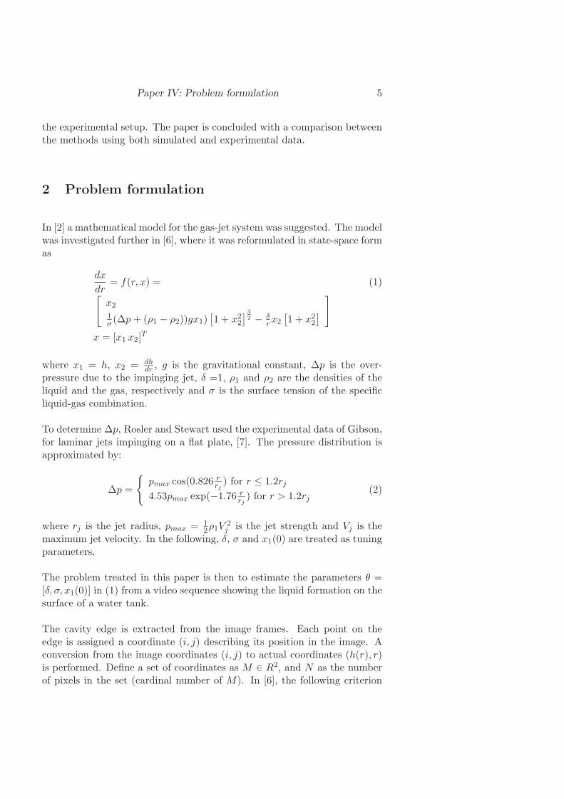
Paper IV: Problem formulation 5
the experimental setup. The paper is concluded with a comparison betweenthe methods using both simulated and experimental data.
2 Problem formulation
In [2] a mathematical model for the gas-jet system was suggested. The modelwas investigated further in [6], where it was reformulated in state-space formas
dx
dr= f(r, x) = (1)
[
x2
1σ (∆p + (ρ1 − ρ2))gx1)
[1 + x2
2
] 32 − δ
rx2
[1 + x2
2
]
]
x = [x1 x2]T
where x1 = h, x2 = dhdr , g is the gravitational constant, ∆p is the over-
pressure due to the impinging jet, δ =1, ρ1 and ρ2 are the densities of theliquid and the gas, respectively and σ is the surface tension of the specificliquid-gas combination.
To determine ∆p, Rosler and Stewart used the experimental data of Gibson,for laminar jets impinging on a flat plate, [7]. The pressure distribution isapproximated by:
∆p =
{
pmax cos(0.826 rrj
) for r ≤ 1.2rj
4.53pmax exp(−1.76 rrj
) for r > 1.2rj(2)
where rj is the jet radius, pmax = 12ρ1V
2j is the jet strength and Vj is the
maximum jet velocity. In the following, δ, σ and x1(0) are treated as tuningparameters.
The problem treated in this paper is then to estimate the parameters θ =[δ, σ, x1(0)] in (1) from a video sequence showing the liquid formation on thesurface of a water tank.
The cavity edge is extracted from the image frames. Each point on theedge is assigned a coordinate (i, j) describing its position in the image. Aconversion from the image coordinates (i, j) to actual coordinates (h(r), r)is performed. Define a set of coordinates as M ∈ R2, and N as the numberof pixels in the set (cardinal number of M). In [6], the following criterion

6 Magnus Evestedt
function is used to estimate the parameters in (1) by optimization.
θ = arg minθ
L(θ) (3)
L(θ) =1
N
∑
r∈M
(h(r) − h(r))2
where h(r) is the model output.
The optimization is performed over the set M , using fminsearch in Matlab c©.In the following, the approach in [6], where all data points, obtained by edgedetection, belong to M , will be referred to as Scheme 1.
The underlying algorithm for the multidimensional unconstrained nonlinearminimization is the Nelder-Mead search, [10]. It is based on evaluating afunction at the vertices of a simplex or hypertetrahedron, then iterativelyshrinking the simplex as better points are found until some desired boundis obtained.
Due to the lack of convergence theory, the efficiency and complexity of theNelder-Mead search algorithm are hard to estimate, [16]. In this particularapplication, the time needed for the algorithm to converge is dependenton the number and placement of the data used in the parameter tuning.The contribution of this paper is two model based approaches to choose thesampling points used in the optimization in such a way that the computationtime is substantially decreased, with acceptable reduction of the estimationaccuracy.
3 Parameter estimation
In this section two alternative model based approaches to decrease the com-putation time of the optimization, by utilizing the data that contain mostinformation about the edge, are presented. The schemes are based on thevital assumption that the cavity shape does not change abruptly from oneframe to another.
3.1 Sampling
The continuous model described by Equation (1) is nonlinear. There isno general theory on how to sample nonlinear systems that can be applied

Paper IV: Parameter estimation 7
directly in this case. Consider a linear second order homogeneous ordinarydifferential equation, which can be seen as a linearization of (1)
y′′(t) + ay′(t) + by(t) = 0 (4)
where the parameters a and b are constant real coefficients. A solution toEquation (4), [15], is given by
y(t) = C1eλ1t + C2e
λ2t (5)
where λ1 and λ2 are negative real numbers and λ1 6= λ2 given by
λ1,2 = −a
2±
√
a2
4− b (6)
In order to obtain a spectrum describing the distribution of energy overfrequency, ω, Equation (5) is readily Fourier transformed as
Y (ω) =C1
jω − λ1+
C2
jω − λ2(7)
According to the sampling theorem (cf Oppenheim and Schafer, 1989) , aband-limited signal (i.e. one with a zero spectrum for frequencies ω > ωB),can be fully reconstructed from its sampled version, if the sampling rate ischosen at least twice as large, that is 2ωB. Normally a much higher samplingrate is recommended, [18].
As can be seen in Equation (7), the spectrum decreases as 1ω . This prop-
erty holds for all solutions to (4). An important user choice when samplingEquation (5) is the threshold, ωB, above which the energy content in the sig-nal can be considered so small that it can be neglected. The reconstructionaccuracy is of course highly dependent upon this choice.
The frequency content of the solution to the nonlinear Equation (1) is moredifficult to characterize. Here, a special feature is utilized, namely the factthat the second state describes the derivative of the indentation profile.Thus, it provides information on how fast the curve changes. This propertyunderlies the following sampling methods.
3.2 An ad-hoc approach
The most interesting points of the indentation profile are where it changesmost rapidly. Studying the derivative of the model adjusted to fit the mea-surement obtained at time t in Figure 3, it can be seen that the derivative

8 Magnus Evestedt
decreases with increasing radial distance r from the origin. The idea is toonly use the points where the derivative exceeds a user-defined threshold inthe optimization of the model parameters to the measurement obtained attime t+1. Thus the amount of data is reduced, decreasing the computationtime.
0 50 100 150 200 250 300−4
−2
0
2
4
6
8
10
12
14x 10
−3
Der
ivat
ive
of h
(r)
r [cm]
Figure 3: The derivative of the model edge.
A summary of the proposed approach is as follows:
Scheme 2
1. Define a threshold, T , for the derivative of the cavity edge w.r.t. r.
2. Take the first frame in the video sequence and extract the edge of thecavity. Let all edge pixels constitute the set M . Solve optimizationproblem (3).
3. Evaluate Equation (1) for the parameters θ(t) obtained in the previousstep to estimate the derivative of the cavity edge w.r.t. r.
4. Find the pixels where the derivative is larger than a user-definedthreshold. Let those points constitute M .
5. Retrieve the next image frame.
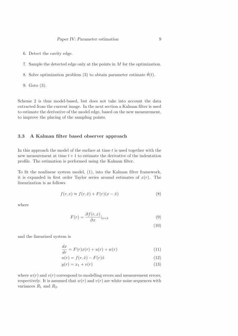
Paper IV: Parameter estimation 9
6. Detect the cavity edge.
7. Sample the detected edge only at the points in M for the optimization.
8. Solve optimization problem (3) to obtain parameter estimate θ(t).
9. Goto (3).
Scheme 2 is thus model-based, but does not take into account the dataextracted from the current image. In the next section a Kalman filter is usedto estimate the derivative of the model edge, based on the new measurement,to improve the placing of the sampling points.
3.3 A Kalman filter based observer approach
In this approach the model of the surface at time t is used together with thenew measurement at time t+1 to estimate the derivative of the indentationprofile. The estimation is performed using the Kalman filter.
To fit the nonlinear system model, (1), into the Kalman filter framework,it is expanded in first order Taylor series around estimates of x(r). Thelinearization is as follows
f(r, x) ≈ f(r, x) + F (r)(x − x) (8)
where
F (r) =∂f(r, x)
∂x|x=x (9)
(10)
and the linearized system is
dx
dr= F (r)x(r) + u(r) + w(r) (11)
u(r) = f(r, x) − F (r)x (12)
y(r) = x1 + v(r) (13)
where w(r) and v(r) correspond to modelling errors and measurement errors,respectively. It is assumed that w(r) and v(r) are white noise sequences withvariances R1 and R2.
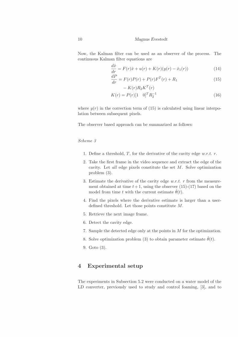
10 Magnus Evestedt
Now, the Kalman filter can be used as an observer of the process. Thecontinuous Kalman filter equations are
dx
dr= F (r)x + u(r) + K(r)(y(r) − x1(r)) (14)
dP
dr= F (r)P (r) + P (r)F T (r) + R1 (15)
− K(r)R2KT (r)
K(r) = P (r)[1 0]T R−12 (16)
where y(r) in the correction term of (15) is calculated using linear interpo-lation between subsequent pixels.
The observer based approach can be summarized as follows:
Scheme 3
1. Define a threshold, T , for the derivative of the cavity edge w.r.t. r.
2. Take the first frame in the video sequence and extract the edge of thecavity. Let all edge pixels constitute the set M . Solve optimizationproblem (3).
3. Estimate the derivative of the cavity edge w.r.t. r from the measure-ment obtained at time t+1, using the observer (15)-(17) based on themodel from time t with the current estimate θ(t).
4. Find the pixels where the derivative estimate is larger than a user-defined threshold. Let those points constitute M .
5. Retrieve the next image frame.
6. Detect the cavity edge.
7. Sample the detected edge only at the points in M for the optimization.
8. Solve optimization problem (3) to obtain parameter estimate θ(t).
9. Goto (3).
4 Experimental setup
The experiments in Subsection 5.2 were conducted on a water model of theLD converter, previously used to study and control foaming, [3], and to

Paper IV: Experimental setup 11
characterize the shape of the cavity, [6]. A single hole cylindrical nozzlewith diameter 1.5 mm was used. The indentation profile arising when air isjetted onto the liquid surface is recorded using a CCD camera. An exampleof a photograph taken with the camera together with an approximation ofthe cavity edge by Equation (1) is shown in Figure 4.
Figure 4: Photograph of the water surface during a blow. An approximationof the cavity edge is included in the image.
4.1 Image processing
To extract the edges from the photographs an in-house software was used,previously employed in [6]. The frames of the video sequence are filteredto reduce the noise in the image. Then edge detection is applied using athresholding method, together with some basic image processing tools suchas opening, closing and flood-fill, [17].
4.2 Sources of error
There are several sources of error in the experimental setup.
• The oxygen flow through the lance is slowly varying with time.

12 Magnus Evestedt
• The lance angle to the water bath cannot be guaranteed to be 90degrees.
• Bubbles and splashing make the edge detection difficult.
5 Results
In this section the three optimization approaches are compared to each otherin terms of approximation accuracy, computation time and data utilization.The comparison is performed on simulated as well as experimental data.
5.1 Simulation results
A sequence of 50 ideal edges obtained from Equation (1) was used to studythe performances of the considered methods. The edge was corrupted usinga white sequence to simulate the random error sources, see Figure 5. Theparameters, θ, were varied in a manner similar to that observed in experi-ments.
0 2 4 6 8 10 12 14 16−3
−2.5
−2
−1.5
−1
−0.5
0
0.5
r [cm]
h(r)
[cm
]
Figure 5: Simulated surface edge.
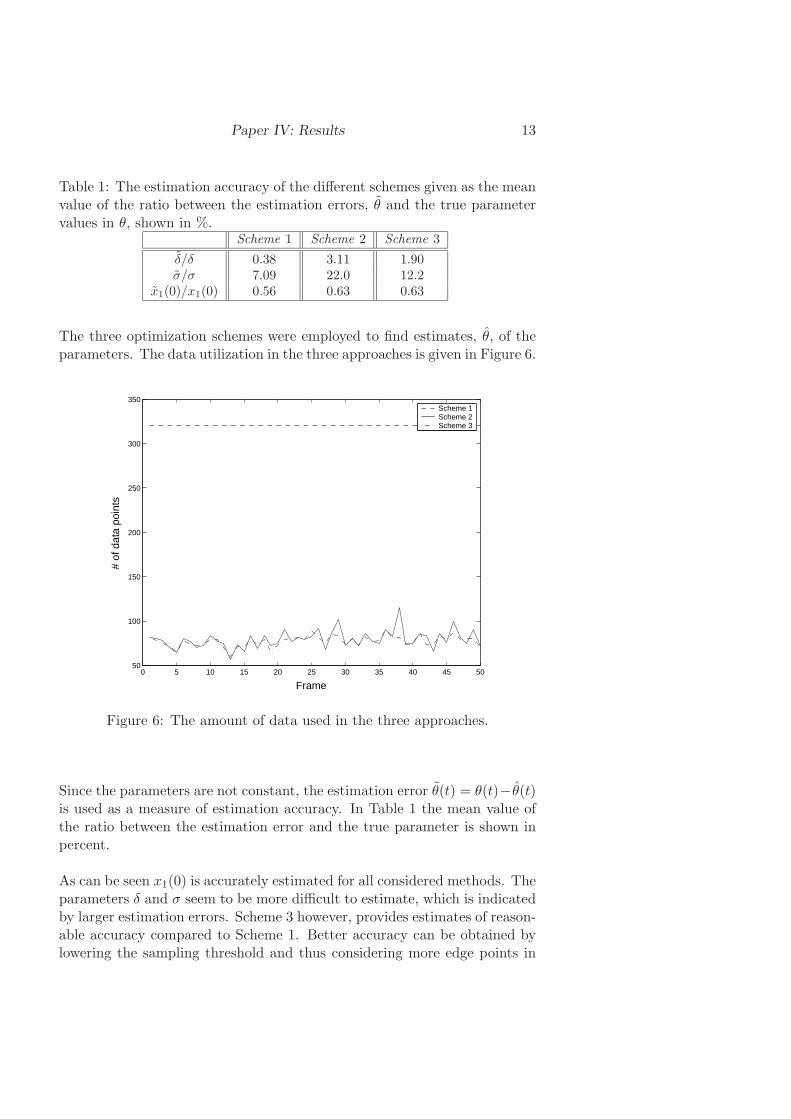
Paper IV: Results 13
Table 1: The estimation accuracy of the different schemes given as the meanvalue of the ratio between the estimation errors, θ and the true parametervalues in θ, shown in %.
Scheme 1 Scheme 2 Scheme 3
δ/δ 0.38 3.11 1.90σ/σ 7.09 22.0 12.2
x1(0)/x1(0) 0.56 0.63 0.63
The three optimization schemes were employed to find estimates, θ, of theparameters. The data utilization in the three approaches is given in Figure 6.
0 5 10 15 20 25 30 35 40 45 5050
100
150
200
250
300
350
Frame
# of
dat
a po
ints
Scheme 1Scheme 2Scheme 3
Figure 6: The amount of data used in the three approaches.
Since the parameters are not constant, the estimation error θ(t) = θ(t)− θ(t)is used as a measure of estimation accuracy. In Table 1 the mean value ofthe ratio between the estimation error and the true parameter is shown inpercent.
As can be seen x1(0) is accurately estimated for all considered methods. Theparameters δ and σ seem to be more difficult to estimate, which is indicatedby larger estimation errors. Scheme 3 however, provides estimates of reason-able accuracy compared to Scheme 1. Better accuracy can be obtained bylowering the sampling threshold and thus considering more edge points in
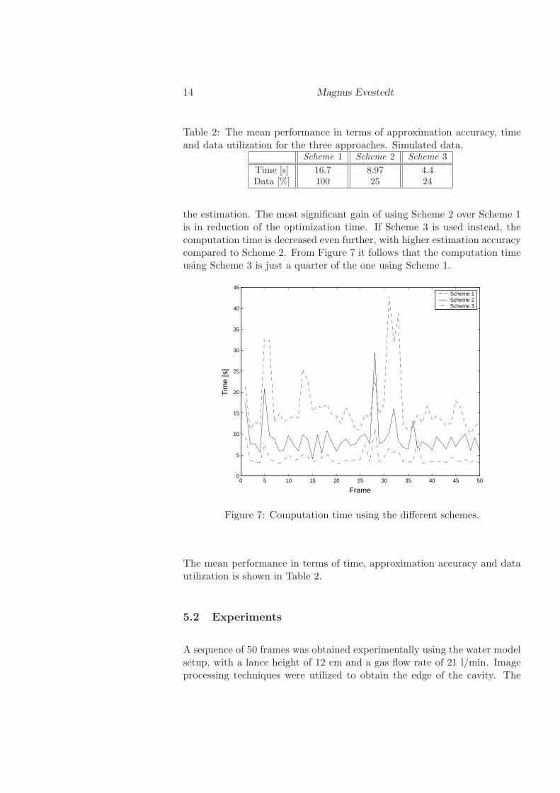
14 Magnus Evestedt
Table 2: The mean performance in terms of approximation accuracy, timeand data utilization for the three approaches. Simulated data.
Scheme 1 Scheme 2 Scheme 3
Time [s] 16.7 8.97 4.4Data [%] 100 25 24
the estimation. The most significant gain of using Scheme 2 over Scheme 1is in reduction of the optimization time. If Scheme 3 is used instead, thecomputation time is decreased even further, with higher estimation accuracycompared to Scheme 2. From Figure 7 it follows that the computation timeusing Scheme 3 is just a quarter of the one using Scheme 1.
0 5 10 15 20 25 30 35 40 45 500
5
10
15
20
25
30
35
40
45
Frame
Tim
e [s
]
Scheme 1Scheme 2Scheme 3
Figure 7: Computation time using the different schemes.
The mean performance in terms of time, approximation accuracy and datautilization is shown in Table 2.
5.2 Experiments
A sequence of 50 frames was obtained experimentally using the water modelsetup, with a lance height of 12 cm and a gas flow rate of 21 l/min. Imageprocessing techniques were utilized to obtain the edge of the cavity. The

Paper IV: Conclusions 15
three approaches, Schemes 1, 2 and Scheme 3, were used to approximate themeasured edge. In Figure 8 the number of data points used in optimizationis shown for the three approaches.
Since true model parameter values are unknown in the experiments, Equa-tion (3) is used as a measure of how well the cavity form is approximated.The full edge measurement is considered as the true edge, h(r), in the lossfunction L(θ). In Figures 9 and 8, the results of the optimization approachesare shown. As can be seen, the reduction of data points does not signifi-cantly affect the performance of the approximation, except at the locationsof the peaks. It is likely that splashing water in the tank destroys the edgedetection and invalidates the model at these points. The best approximationin this case is naturally the approach using all the measured data.
The gain in computation time achieved by using Schemes 2 and 3 insteadof Scheme 1 is illustrated in Figure 10.
The mean performance in terms of time, approximation accuracy and datautilization is shown in Table 3. The large peaks for some of the edge realiza-tions affect the mean values significantly, explaining the large mean valuesof L(θ) in Scheme 2 and Scheme 3.
Table 3: The mean performance in terms of approximation accuracy, timeand data utilization for the three approaches. Experimental data.
Scheme 1 Scheme 2 Scheme 3
L 0.015 13.6 0.41Time [s] 38.5 33.3 27.4Data [%] 100 63 61
6 Conclusions
Two approaches to selecting sampling points in a nonuniform way in theimages of a surface cavity in a water model were proposed. Instead of usingall the data points, a smaller number of data was utilized and shown bothon simulated as well as on experimental data to decrease the computationtime with an acceptable reduction of the estimation accuracy.

16 Magnus Evestedt
0 5 10 15 20 25 30 35 40 45 5060
80
100
120
140
160
180
200
Frame
# of
dat
a po
ints
Scheme 1Scheme 2Scheme 3
Figure 8: The amount of data used in the three approaches.
0 5 10 15 20 25 30 35 40 45 500
0.5
1
1.5
2
2.5
3
3.5
4
4.5
5
Frame
L
Scheme 1Scheme 2Scheme 3
Figure 9: The approximation accuracy for the three optimization approachesusing 50 realizations of the edge.
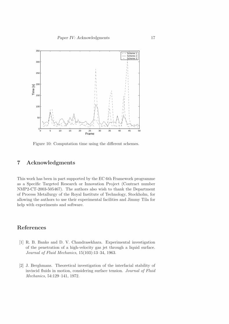
Paper IV: Acknowledgments 17
0 5 10 15 20 25 30 35 40 45 500
50
100
150
200
250
300
350
Frame
Tim
e [s
]
Scheme 1Scheme 2Scheme 3
Figure 10: Computation time using the different schemes.
7 Acknowledgments
This work has been in part supported by the EC 6th Framework programmeas a Specific Targeted Research or Innovation Project (Contract numberNMP2-CT-2003-505467). The authors also wish to thank the Departmentof Process Metallurgy of the Royal Institute of Technology, Stockholm, forallowing the authors to use their experimental facilities and Jimmy Tila forhelp with experiments and software.
References
[1] R. B. Banks and D. V. Chandrasekhara. Experimental investigationof the penetration of a high-velocity gas jet through a liquid surface.Journal of Fluid Mechanics, 15(103):13–34, 1963.
[2] J. Berghmans. Theoretical investigation of the interfacial stability ofinviscid fluids in motion, considering surface tension. Journal of FluidMechanics, 54:129–141, 1972.

18 Magnus Evestedt
[3] W. Birk, I. Arvanitidis, P. Jonsson, and A. Medvedev. Foam level con-trol in a water model of the LD converter process. Control EngineeringPractice, 11:49–56, 2003.
[4] F. R. Cheslak, J. A. Nicholls, and M. Sichel. Cavities formed on liquidsurfaces by impinging gaseous jets. Journal of Fluid Mechanics, 36:55–64, 1969.
[5] S. Eletribi, D. K. Mukherjee, and V. Prasad. Experiments on liquidsurface deformation upon impingement by a gas jet. In Proceedings ofthe ASME Fluids Engineering Division, volume 244, 1997.
[6] M. Evestedt and A. Medvedev. Gas jet impinging on liquid surface:Cavity shape modelling and estimation. In Proceedings of the 16thIFAC World Congress, July 2005.
[7] A. H. Gibson. Hydraulics and Its Application. London:Constable, 1934.
[8] M. S. Lee, S. L. O´Rourke, and N. A. Molloy. Fluid flow and surfacewaves in the BOF. ISS Transactions, 29(10):56–65, 2002.
[9] N. A. Molloy. Impinging jet flow in a two-phase system:the basic flowpattern. Journal of the iron and steel institute, pages 943–950, October1970.
[10] J. A. Nelder and R. Mead. A simplex method for function minimization.Computer Journal, 7:308–313, 1965.
[11] A. Nordquist. A physical modeling study of top blowing with focus onthe penetration region. Licentiate thesis, Royal institute of technology,Stockholm, Sweden, 2005.
[12] W. E. Olmstead and S. Raynor. Depression of an infinite liquid surfaceby an incompressible gas jet. Journal of Fluid Mechanics, 19:561–576,1964.
[13] A. V. Oppenheim and R. W. Schafer. Discrete-Time Signal Processing.Prentice Hall, 1989.
[14] R. S. Rosler and G. H. Stewart. Impingement of gas jets on liquidsurfaces. Journal of Fluid Mechanics, 31:163–174, 1968.
[15] G. F. Simmons. Differential equations with applications and historicalnotes. McGraw Hill, Inc, 1991.
[16] S. Singer and S. Singer. Efficient implementation of the Nelder-Meadsearch algorithm. Applied Numerical Analysis & Computational Math-ematics, 1:524–534, 2004.
Paper IV: Acknowledgments 19
[17] M. Sonka, V. Hlavac, and R. Boyle. Image processing, analysis andmachine vision. PWS Publishing, 1999.
[18] K. J. Astrom and B. Wittenmark. Computer-controlled systems. Pren-tice Hall, 1997.
[19] E. T. Turkdogan. Fluid dynamics of gas jets impinging on surface ofliquids. Chemical Engineering Science, 21:1133–1144, 1966.
[20] J. M. Vanden-Broeck. Deformation of a liquid surface by an impinginggas jet. SIAM Journal of Applied Mathematics, 41(2):306–309, 1981.
[21] Steel industry technology roadmap. www.steel.org, June 2005.


Recent licentiate theses from the Department of Information Technology
2004-003 Yngve Selen: Model Selection
2004-004 Mohammed El Shobaki: On-Chip Monitoring for Non-Intrusive Hard-ware/Software Observability
2004-005 Henrik Lof: Parallelizing the Method of Conjugate Gradients for Shared Mem-ory Architectures
2004-006 Stefan Johansson:High Order Difference Approximations for the LinearizedEuler Equations
2005-001 Jesper Wilhelmsson:Efficient Memory Management for Message-PassingConcurrency — part I: Single-threaded execution
2005-002 Hakan Zeffer:Hardware-Software Tradeoffs in Shared-Memory Implementa-tions
2005-003 MagnusAgren: High-Level Modelling and Local Search
2005-004 Oskar Wibling:Ad Hoc Routing Protocol Validation
2005-005 Peter Naucler: Modeling and Control of Vibration in Mechanical Structures
2005-006 Erik Bangtsson:Robust Preconditioned Iterative Solution Methods for Large-Scale Nonsymmetric Problems
2005-007 Mei Hong: On Two Methods for Identifying Dynamic Errors-in-VariablesSys-tems
2005-008 Niklas Johansson:Usable IT Systems for Mobile Work
2005-009 Magnus Evestedt:Parameter and State Estimation using Audio and Video Sig-nals
Department of Information Technology, Uppsala University, Sweden