Parallel Processing - bs. · PDF fileBetriebssysteme / verteilte Systeme Parallel Processing...
515
Roland Wism¨ uller Betriebssysteme / verteilte Systeme Parallel Processing (1/17) i Roland Wism ¨ uller Universit ¨ at Siegen rolanda .d wismuellera @d uni-siegena .d de Tel.: 0271/740-4050, B¨ uro: H-B 8404 Stand: January 23, 2018 Parallel Processing WS 2017/18
Transcript of Parallel Processing - bs. · PDF fileBetriebssysteme / verteilte Systeme Parallel Processing...
Roland WismullerBetriebssysteme / verteilte Systeme Parallel Processing (1/17) i
Roland Wismuller
Universitat Siegen
Tel.: 0271/740-4050, Buro: H-B 8404
Stand: January 23, 2018
Parallel Processing
WS 2017/18

Roland WismullerBetriebssysteme / verteilte Systeme Parallel Processing (1/17) 2
Parallel ProcessingWS 2017/18
0 Organisation
About Myself
Roland WismullerBetriebssysteme / verteilte Systeme Parallel Processing (1/17) 3
➥ Studies in Computer Science, Techn. Univ. Munich
➥ Ph.D. in 1994, state doctorate in 2001
➥ Since 2004 Prof. for Operating Systems and Distributed Systems
➥ Research: Monitoring, Analysis und Control of parallel and
distributed Systems
➥ Mentor for Bachelor Studies in Computer Science with secondary
field Mathematics
➥ E-mail: [email protected]
➥ Tel.: 0271/740-4050
➥ Room: H-B 8404
➥ Office Hour: Mo., 14:15-15:15 Uhr
About the Chair ”‘Operating Systems / Distrib. Sys.”’
Roland WismullerBetriebssysteme / verteilte Systeme Parallel Processing (1/17) 4
Andreas Hoffmannandreas.hoffmann@uni-...
0271/740-4047
H-B 8405
➥ E-assessment and e-labs
➥ IT security
➥ Web technologies
➥ Mobile applications
Damian Ludwigdamian.ludwig@uni-...
0271/740-2533
H-B 8402
➥ Capability systems
➥ Compilers
➥ Programming languages
Alexander Kordesalexander.kordes@uni-...
0271/740-4011
H-B 8407
➥ Automotive electronics
➥ In-car networks
➥ Pattern recognition in car sensordata
Teaching
Roland WismullerBetriebssysteme / verteilte Systeme Parallel Processing (1/17) 5
Lectures/Labs
➥ Rechnernetze I, 5 LP (every summer term)
➥ Rechnernetze Praktikum, 5 LP (every winter term)
➥ Rechnernetze II, 5 LP (every summer term)
➥ Betriebssysteme I, 5 LP (every winter term)
➥ Parallelverarbeitung, 5 LP (every winter term)
➥ Verteilte Systeme, 5 LP (every summer term)
➥ (will be recognised as Betriebssysteme II)
➥ Client/Server-Programmierung, 5 LP (every winter term)
Teaching ...
Roland WismullerBetriebssysteme / verteilte Systeme Parallel Processing (1/17) 6
Project Groups
➥ e.g., tool for visualization of algorithms
➥ e.g., infrastructure for analysing the Android market
Theses (Bachelor, Master)
➥ Topic areas: mobile plattforms (iOS, Android), sensor networks,parallel computing, pattern recognition in sensor data, security, ...
➥ e.g., static information flow analysis of Android apps
Seminars
➥ Topic areas: web technologies, sensor networks, patternrecognition in sensor data, ...
➥ Procedure: block seminar
➥ 30 min. talk, 5000 word seminar paper
About the Lecture
Roland WismullerBetriebssysteme / verteilte Systeme Parallel Processing (1/17) 7
➥ Lecture + practical Labs: 2+2 SWS, 5 LP
➥ Tutor: Matthias Bundschuh
➥ Date and Time:
➥ Mon. 12:30 - 14:00, H-F 001 (Lect.) or H-A 4111 (Lab)
➥ Thu. 16:00 - 17:30, ??????? (Lect.) or H-A 4111 (Lab)
➥ Information, slides, and announcements:
➥ in the WWW: http://www.bs.informatik.uni-siegen.de/lehre/ws1718/pv/
➥ annotated slides (PDF) available; maybe slight modifications
➥ updated slides will normally be published at least one daybefore the lecture
➥ code examples are installed locally on the lab computers in/home/wismueller/PV

About the Lecture ...
Roland WismullerBetriebssysteme / verteilte Systeme Parallel Processing (1/17) 8
Learning targets
➥ Knowing the basics, techniques, methods, and tools of parallelprogramming
➥ Basic knowledge about parallel computer architectures
➥ Practical experiences with parallel programming
➥ Knowing and being able to use the most important programmingmodels
➥ Knowing about the possibilities, difficulties and limits of parallelprocessing
➥ Being able to identify and select promising strategies forparallelization
➥ Focus: high performance computing
About the Lecture ...
Roland WismullerBetriebssysteme / verteilte Systeme Parallel Processing (1/17) 9
Methodology
➥ Lecture: Basics
➥ theoretical knowledge about parallel processing
➥ Lab: practical use
➥ practical introduction to programming environments
➥ ”’hands-on”’ tutorials
➥ independent programming work
➥ practical skills and experiences
➥ in addition: raising questions
➥ different parallelizations of two representative problems
➥ iterative, numerical method
➥ combinatoral search
Examination
Roland WismullerBetriebssysteme / verteilte Systeme Parallel Processing (1/17) 10
➥ Oral examination (about 30-40 min.)
➥ subject matter: lecture and labs!
➥ examination also covers the practical exercises
➥ Prerequisite for admission: active attendance to the labs
➥ i.e., qualified attempt for all main exercises
➥ Application:
➥ fix a date with my secretary Mrs. Syska
➥ via email ([email protected])
➥ or personally (H-B 8403, in the morning)
➥ application at the examination office

Insertion: Important Notice
Roland WismullerBetriebssysteme / verteilte Systeme Parallel Processing (1/17) ii
For Computer Science Students
➥ Please note the deadlines of the examination office:
➥ filing of the “Personalbogen”: 10.11.2017
➥ filing of the “Mentorengenehmigung”: 23.11.2017
➥ without the “Mentorengenehmigung” you cannot enroll forexaminations in non-obligatory courses!
➥ enrollment for written exams: 04.12. - 21.12.2017➥ you can unsubscribe up to one week before the exam
➥ (oral exams: no deadline for enrollment)
➥ Deadlines are earlier just in the winter term 2017/18
➥ in January, the campus management system will be replaced!
➥ Other students (esp. business informatics, teaching):
➥ please inform yourself at your examination office!
Organisational Issues regarding the Labs
Roland WismullerBetriebssysteme / verteilte Systeme Parallel Processing (1/17) 11
➥ User regulations and key card application form:
➥ http://www.bs.informatik.uni-siegen.de/lehre/
ws1718/pv/
➥ please let me sign the key card application form and then
deliver it directly to Mr. Kiel (AR-P 209)
➥ Start of labs: 02.11.
➥ introduction to the computer environment (Linux)
➥ emission of login credentials
➥ please pay attention to the user regulations in the WWW!
➥ Programming in C/C++
Computer Environment in the Lab Room H-A 4111
Roland WismullerBetriebssysteme / verteilte Systeme Parallel Processing (1/17) 12
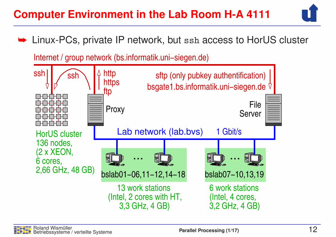
➥ Linux-PCs, private IP network, but ssh access to HorUS cluster
2,66 GHz, 48 GB)6 cores,(2 x XEON, 136 nodes,HorUS cluster
13 work stations(Intel, 2 cores with HT,
3,3 GHz, 4 GB) 3,2 GHz, 4 GB)
6 work stations(Intel, 4 cores,
httphttpsftp
ssh ssh
Internet / group network (bs.informatik.uni−siegen.de)
sftp (only pubkey authentification)
bsgate1.bs.informatik.uni−siegen.de
Lab network (lab.bvs) 1 Gbit/s
FileServer
Proxy
...
bslab01−06,11−12,14−18
...
bslab07−10,13,19
��������
����
����
��������
Contents of the Lecture
Roland WismullerBetriebssysteme / verteilte Systeme Parallel Processing (1/17) 13
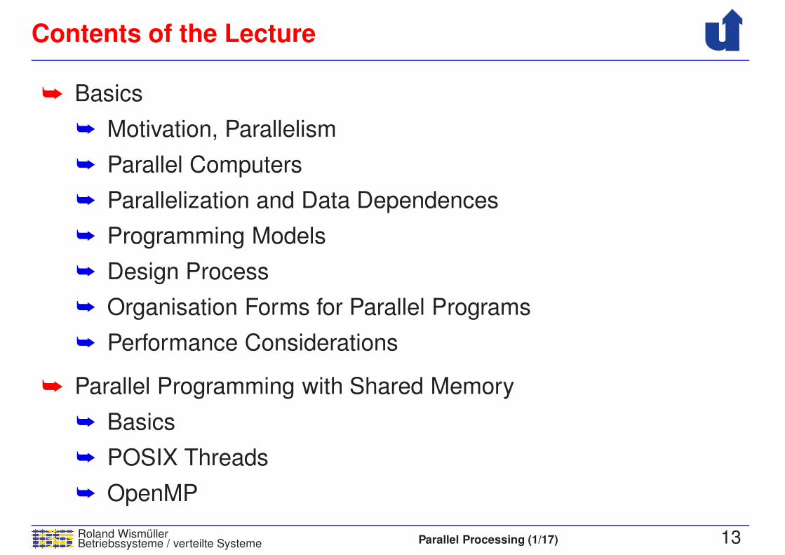
➥ Basics
➥ Motivation, Parallelism
➥ Parallel Computers
➥ Parallelization and Data Dependences
➥ Programming Models
➥ Design Process
➥ Organisation Forms for Parallel Programs
➥ Performance Considerations
➥ Parallel Programming with Shared Memory
➥ Basics
➥ POSIX Threads
➥ OpenMP
Contents of the Lecture ...
Roland WismullerBetriebssysteme / verteilte Systeme Parallel Processing (1/17) 14
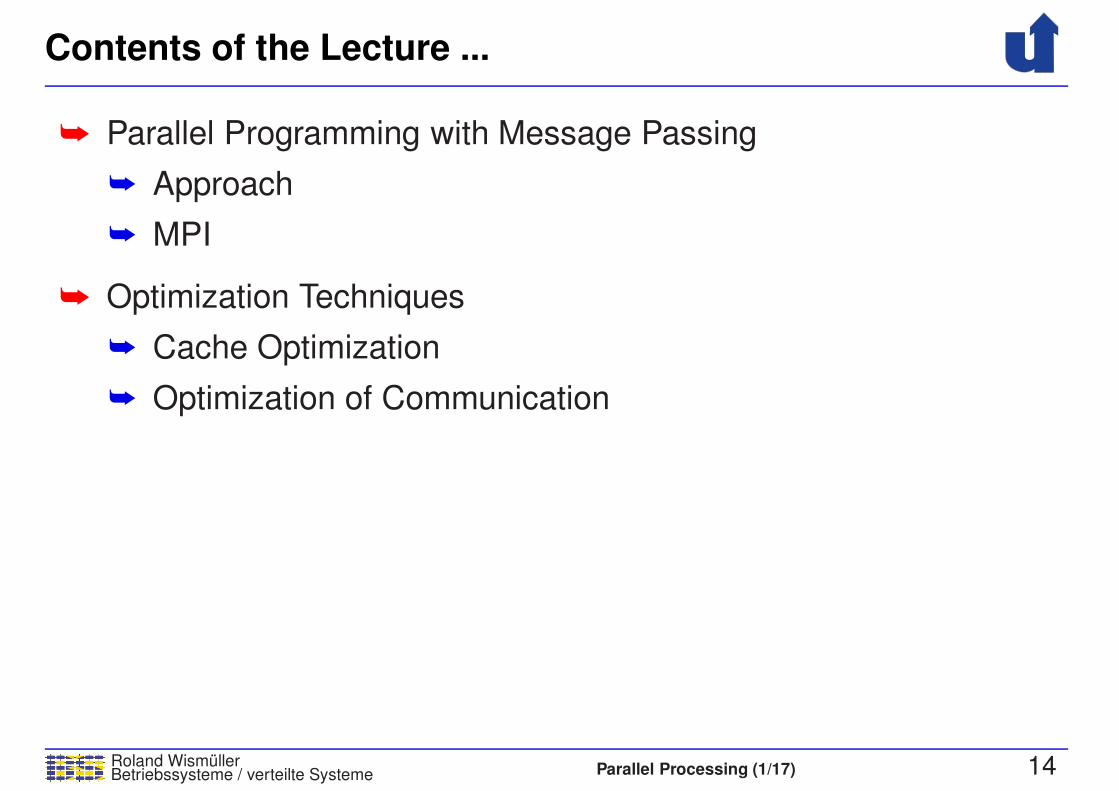
➥ Parallel Programming with Message Passing
➥ Approach
➥ MPI
➥ Optimization Techniques
➥ Cache Optimization
➥ Optimization of Communication
Preliminary Time Table of Lecture (V) and Labs (U)
Roland WismullerBetriebssysteme / verteilte Systeme Parallel Processing (1/17) 15
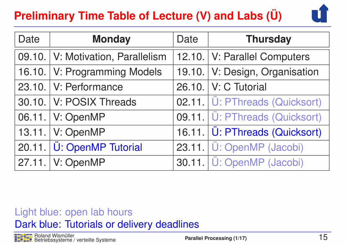
Date Monday Date Thursday
09.10. V: Motivation, Parallelism 12.10. V: Parallel Computers
16.10. V: Programming Models 19.10. V: Design, Organisation
23.10. V: Performance 26.10. V: C Tutorial
30.10. V: POSIX Threads 02.11. U: PThreads (Quicksort)
06.11. V: OpenMP 09.11. U: PThreads (Quicksort)
13.11. V: OpenMP 16.11. U: PThreads (Quicksort)
20.11. U: OpenMP Tutorial 23.11. U: OpenMP (Jacobi)
27.11. V: OpenMP 30.11. U: OpenMP (Jacobi)
Light blue: open lab hours
Dark blue: Tutorials or delivery deadlines

Preliminary Time Table of Lecture (V) and Labs (U) ...
Roland WismullerBetriebssysteme / verteilte Systeme Parallel Processing (1/17) 16
Date Monday Date Thursday
04.12. U: Sokoban 07.12. U: OpenMP (Jacobi)
11.12. V: MPI 14.12. U: OpenMP (Jacobi)
18.12. V: MPI 21.12. U: OpenMP (Sokoban)
08.01. V: MPI 11.01. U: OpenMP (Sokoban)
15.01. U: MPI Tutorial 18.01. U: OpenMP (Sokoban))
22.01. V: Optimization 25.02. U: MPI (Jacobi)
02.02. U: MPI (Jacobi) 01.02. U: MPI (Jacobi)
Light blue: open lab hours
Dark blue: Tutorials or delivery deadlines

General Literature
Roland WismullerBetriebssysteme / verteilte Systeme Parallel Processing (1/17) 17
➥ Currently no recommendation for a all-embracing text book
➥ Barry Wilkinson, Michael Allen: Parallel Programming. internat.
ed, 2. ed., Pearson Education international, 2005.
➥ covers most parts of the lecture, many examples
➥ short references for MPI, PThreads, OpenMP
➥ A. Grama, A. Gupta, G. Karypis, V. Kumar: Introduction to Parallel
Computing, 2nd Edition, Pearson, 2003.
➥ much about design, communication, parallel algorithms
➥ Thomas Rauber, Gudula Runger: Parallele Programmierung.
2. Auflage, Springer, 2007.
➥ architecture, programming, run-time analysis, algorithms

General Literature ...
Roland WismullerBetriebssysteme / verteilte Systeme Parallel Processing (1/17) 18
➥ Theo Ungerer: Parallelrechner und parallele Programmierung,
Spektrum, Akad. Verl., 1997.
➥ much about parallel hardware and operating systems
➥ also basics of programming (MPI) and compiler techniques
➥ Ian Foster: Designing and Building Parallel Programs,
Addison-Wesley, 1995.
➥ design of parallel programs, case studies, MPI
➥ Seyed Roosta: Parallel Processing and Parallel Algorithms,
Springer, 2000.
➥ mostly algorithms (design, examples)
➥ also many other approaches to parallel programming

Literature for Special Topics
Roland WismullerBetriebssysteme / verteilte Systeme Parallel Processing (1/17) 19
➥ S. Hoffmann, R.Lienhart: OpenMP, Springer, 2008.
➥ handy pocketbook on OpenMP
➥ W. Gropp, E. Lusk, A. Skjellum: Using MPI, MIT Press, 1994.
➥ the definitive book on MPI
➥ D.E. Culler, J.P. Singh: Parallel Computer Architecture - A
Hardware / Software Approach. Morgan Kaufmann, 1999.
➥ UMA/NUMA systems, cache coherency, memory consistency
➥ Michael Wolfe: Optimizing Supercompilers for Supercomputers,MIT Press, 1989.
➥ details on parallelizing compilers
Roland WismullerBetriebssysteme / verteilte Systeme Parallel Processing (1/17) 20
Parallel ProcessingWS 2017/18
1 Basics
1 Basics ...
Roland WismullerBetriebssysteme / verteilte Systeme Parallel Processing (1/17) 21
Contents
➥ Motivation
➥ Parallelism
➥ Parallel computer architectures
➥ Parallel programming models
➥ Performance and scalability of parallel programs
➥ Strategies for parallelisation
➥ Organisation forms for parallel programs
Literature
➥ Ungerer
➥ Grama, Gupta, Karypis, Kumar
1.1 Motivation
Roland WismullerBetriebssysteme / verteilte Systeme Parallel Processing (1/17) 22
What is parallelism?
➥ In general:
➥ executing more than one action at a time
➥ Specifically with respect to execution of programs:
➥ at some point in time
➥ more than one statement is executed
and / or
➥ more than one pair of operands is processed
➥ Goal: faster solution of the task to be processed
➥ Problems: subdivision of the task, coordination overhead
1.1 Motivation ...
Roland WismullerBetriebssysteme / verteilte Systeme Parallel Processing (1/17) 23
Why parallel processing?
➥ Applications with high computing demands, esp. simulations
➥ climate, earthquakes, superconductivity, molecular design, ...
➥ Example: protein folding
➥ 3D structure, function of proteins (Alzheimer, BSE, ...)
➥ 1, 5 · 1011 floating point operations (Flop) / time step
➥ time step: 5 · 10−15s
➥ to simulate: 10−3s
➥ 3 · 1022 Flop / simulation
➥ ⇒ 1 year computation time on a PFlop/s computer!
➥ For comparison: world’s currently fastest computer: Sunway
TaihuLight (China), 93 PFlop/s (with 10.649.600 CPU cores!)
1.1 Motivation ...
Roland WismullerBetriebssysteme / verteilte Systeme Parallel Processing (1/17) 24
Why parallel processing? ...
➥ Moore’s Law: the computing power of a processor doubles every
18 months
➥ but: memory speed increases much slower
➥ 2040 the latest: physical limit will be reached
➥ Thus:
➥ high performance computers are based on parallel processing
➥ even standard CPUs use parallel processing internally
➥ super scalar processors, pipelining, multicore, ...
➥ Economic advantages of parallel computers
➥ cheap standard CPUs instead of specifically developed ones
1.1 Motivation ...
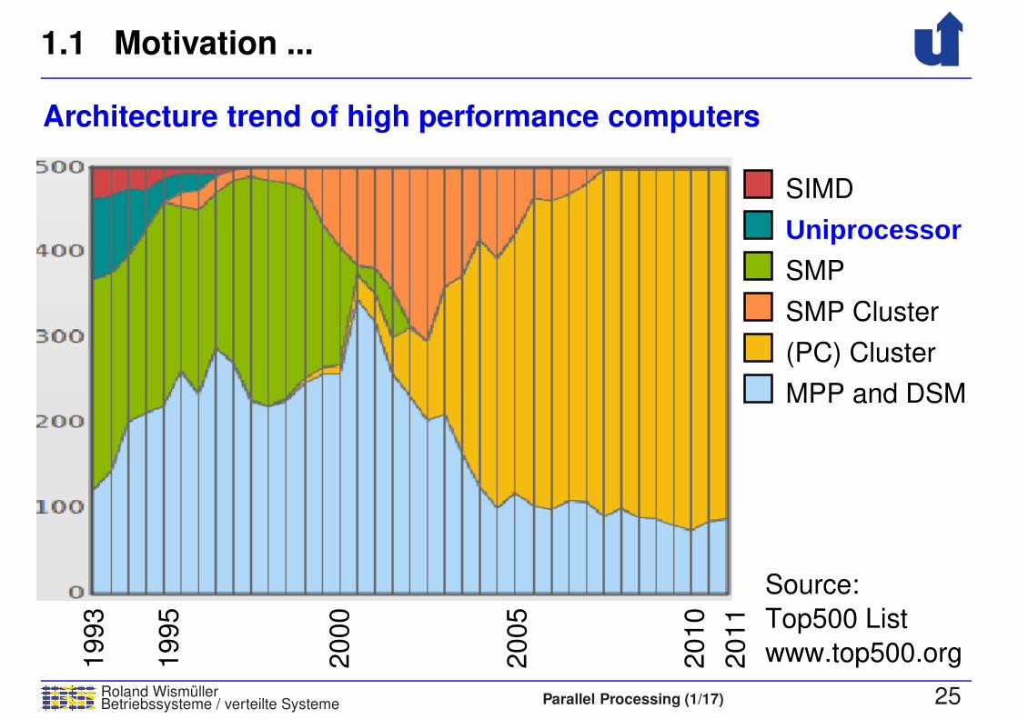
Roland WismullerBetriebssysteme / verteilte Systeme Parallel Processing (1/17) 25
Architecture trend of high performance computers1993
1995
2000
2005
2010
2011
Source:
Top500 List
www.top500.org
SMP
SIMD
Uniprocessor
SMP Cluster
MPP and DSM
(PC) Cluster
1.2 Parallelism
Roland WismullerBetriebssysteme / verteilte Systeme Parallel Processing (1/17) 26
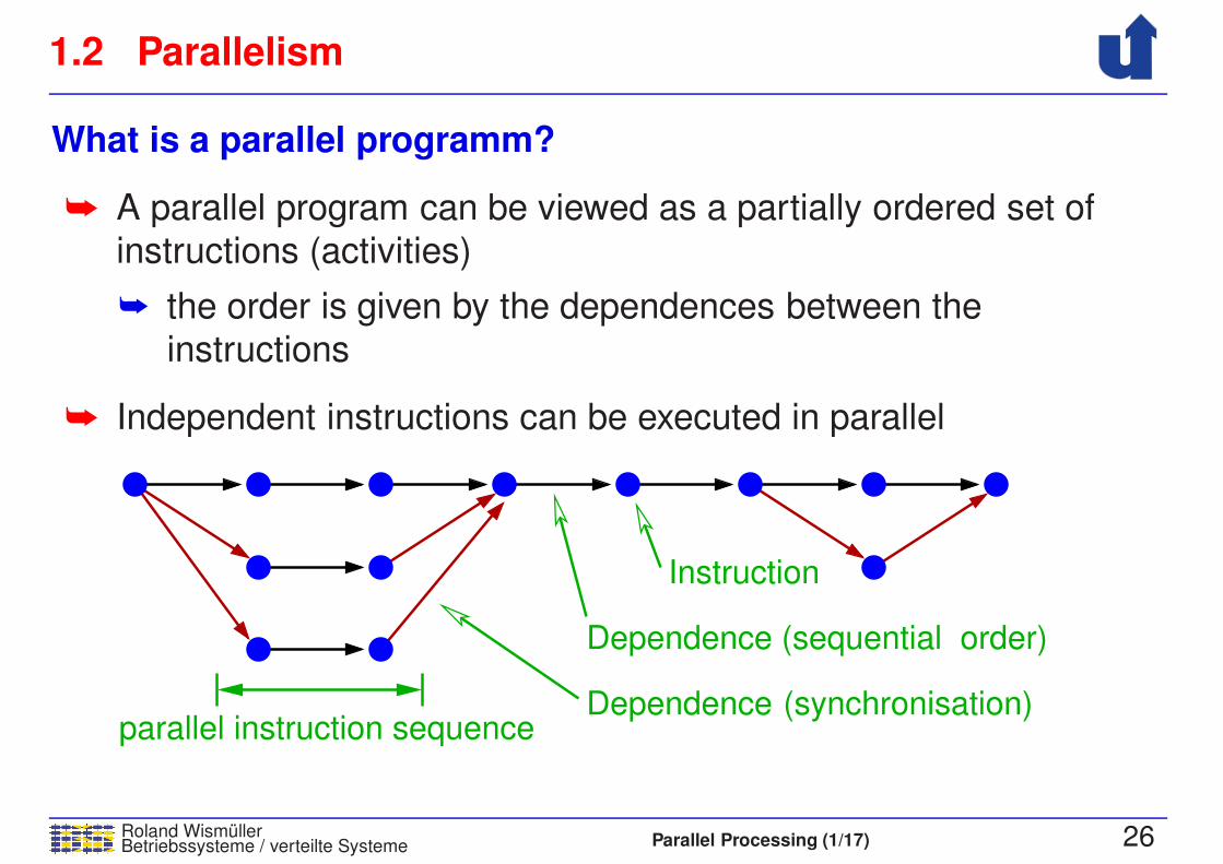
What is a parallel programm?
➥ A parallel program can be viewed as a partially ordered set of
instructions (activities)
➥ the order is given by the dependences between the
instructions
➥ Independent instructions can be executed in parallel
Dependenceparallel instruction sequence
(synchronisation)
Instruction
Dependence (sequential order)
1.2 Parallelism ...
Roland WismullerBetriebssysteme / verteilte Systeme Parallel Processing (1/17) 27
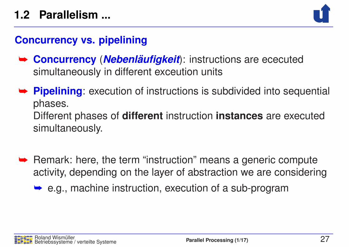
Concurrency vs. pipelining
➥ Concurrency (Nebenlaufigkeit): instructions are ececuted
simultaneously in different exceution units
➥ Pipelining: execution of instructions is subdivided into sequential
phases.
Different phases of different instruction instances are executed
simultaneously.
➥ Remark: here, the term “instruction” means a generic compute
activity, depending on the layer of abstraction we are considering
➥ e.g., machine instruction, execution of a sub-program

1.2 Parallelism ...
Roland WismullerBetriebssysteme / verteilte Systeme Parallel Processing (1/17) 28
Concurrency vs. pipelining ...
SequentialExecution
Concurrent
Execution
(2 Stages)
Pipelining
B C DA
A C
B D
A1 B1 C1 D1
A2 B2 C2 D2
1.2 Parallelism ...
Roland WismullerBetriebssysteme / verteilte Systeme Parallel Processing (1/17) 29
At which layers of programming can we use parallelism?
➥ There is no consistent classification
➥ E.g., layers in the book from Waldschmidt, Parallelrechner:
Architekturen - Systeme - Werkzeuge, Teubner, 1995:
➥ application programs
➥ cooperating processes
➥ data structures
➥ statements and loops
➥ machine instruction
“They are heterogeneous, subdivided according to different
characteristics, and partially overlap.”
1.2 Parallelism ...
Roland WismullerBetriebssysteme / verteilte Systeme Parallel Processing (1/17) 30
View of the application developer (design phase):
➥ “Natural parallelism”
➥ e.g., computing the foces for all stars of a galaxy
➥ often too fine-grained
➥ Data parallelism (domain decomposition, Gebietsaufteilung)
➥ e.g., sequential processing of all stars in a space region
➥ Task parallelism
➥ e.g., pre-processing, computation, post-processing,
visualisation

Roland WismullerBetriebssysteme / verteilte Systeme Parallel Processing (2/17) iii
Roland Wismuller
Universitat Siegen
Tel.: 0271/740-4050, Buro: H-B 8404
Stand: January 23, 2018
Parallel Processing
WS 2017/18
12.10.2017
1.2 Parallelism ...
Roland WismullerBetriebssysteme / verteilte Systeme Parallel Processing (2/17) 31
View of the programmer:
➥ Explicit parallelism
➥ exchange of data (communication / synchronisation) must be
explicitly programmed
➥ Implicit parallelism
➥ by the compiler
➥ directive controlled or automatic
➥ loop level / statement level
➥ compiler generates code for cmmunication
➥ within a CPU (that appears to be sequential from the outside)
➥ super scalar processor, pipelining, ...
1.2 Parallelism ...
Roland WismullerBetriebssysteme / verteilte Systeme Parallel Processing (2/17) 32
View of the system (computer / operating system):
➥ Program level (job level)
➥ independent programs
➥ Process level (task level)
➥ cooperating processes
➥ mostly with explicit exchange of messages
➥ Block level
➥ light weight processes (threads)
➥ communication via shared memory
➥ often created by the compiler
➥ parallelisation of loops
1.2 Parallelism ...
Roland WismullerBetriebssysteme / verteilte Systeme Parallel Processing (2/17) 33
View of the system (computer / operating system): ...
➥ Instruction level
➥ elementary instructions (operations that cannot be further
subdivided in the programming language)
➥ scheduling is done automatically by the compiler and/or by the
hardware at runtime
➥ e.g., in VLIW (EPIC) and super scalar processors
➥ Sub-operation level
➥ compiler or hardware subdivide elementary instructions into
sub-operations that are executed in parallel
➥ e.g., with vector or array operations
1.2 Parallelism ...
Roland WismullerBetriebssysteme / verteilte Systeme Parallel Processing (2/17) 34
Granularity
➥ Defined by the ratio between computation and communication
(including synchronisation)
➥ intuitively, this corresponds to the length of the parallel
instruction sequences in the partial order
➥ determines the requirements for the parallel computer
➥ especially its communication system
➥ influences the achievable acceleration (Speedup)
➥ Coarse-grained: Program and Process level
➥ Mid-grained: block level
➥ Fine-grained: instruction level

1.3 Parallelisation and Data Dependences
Roland WismullerBetriebssysteme / verteilte Systeme Parallel Processing (2/17) 35
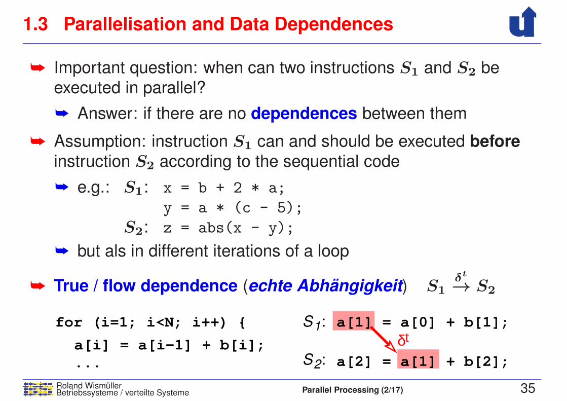
➥ Important question: when can two instructions S1 and S2 be
executed in parallel?
➥ Answer: if there are no dependences between them
➥ Assumption: instruction S1 can and should be executed beforeinstruction S2 according to the sequential code
➥ e.g.: S1: x = b + 2 * a;
y = a * (c - 5);
S2: z = abs(x - y);
➥ but als in different iterations of a loop
➥ True / flow dependence (echte Abhangigkeit) S1δt
→ S2
for (i=1; i<N; i++) {
a[i] = a[i−1] + b[i];
...

1.3 Parallelisation and Data Dependences
Roland WismullerBetriebssysteme / verteilte Systeme Parallel Processing (2/17) 35
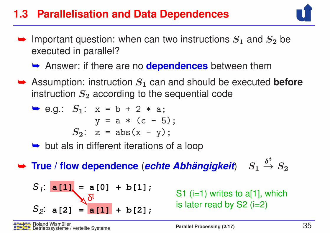
➥ Important question: when can two instructions S1 and S2 be
executed in parallel?
➥ Answer: if there are no dependences between them
➥ Assumption: instruction S1 can and should be executed beforeinstruction S2 according to the sequential code
➥ e.g.: S1: x = b + 2 * a;
y = a * (c - 5);
S2: z = abs(x - y);
➥ but als in different iterations of a loop
➥ True / flow dependence (echte Abhangigkeit) S1δt
→ S2
S1:
S2: a[2] = a[1] + b[2];
a[1] = a[0] + b[1];for (i=1; i<N; i++) {
a[i] = a[i−1] + b[i];
...
1.3 Parallelisation and Data Dependences
Roland WismullerBetriebssysteme / verteilte Systeme Parallel Processing (2/17) 35
➥ Important question: when can two instructions S1 and S2 be
executed in parallel?
➥ Answer: if there are no dependences between them
➥ Assumption: instruction S1 can and should be executed beforeinstruction S2 according to the sequential code
➥ e.g.: S1: x = b + 2 * a;
y = a * (c - 5);
S2: z = abs(x - y);
➥ but als in different iterations of a loop
➥ True / flow dependence (echte Abhangigkeit) S1δt
→ S2
δt
S1:
S2: a[2] = a[1] + b[2];
a[1] = a[0] + b[1];for (i=1; i<N; i++) {
a[i] = a[i−1] + b[i];
...
1.3 Parallelisation and Data Dependences
Roland WismullerBetriebssysteme / verteilte Systeme Parallel Processing (2/17) 35
➥ Important question: when can two instructions S1 and S2 be
executed in parallel?
➥ Answer: if there are no dependences between them
➥ Assumption: instruction S1 can and should be executed beforeinstruction S2 according to the sequential code
➥ e.g.: S1: x = b + 2 * a;
y = a * (c - 5);
S2: z = abs(x - y);
➥ but als in different iterations of a loop
➥ True / flow dependence (echte Abhangigkeit) S1δt
→ S2
S1 (i=1) writes to a[1], which
is later read by S2 (i=2)δt
S1:
S2: a[2] = a[1] + b[2];
a[1] = a[0] + b[1];

1.3 Parallelisation and Data Dependences ...
Roland WismullerBetriebssysteme / verteilte Systeme Parallel Processing (2/17) 36
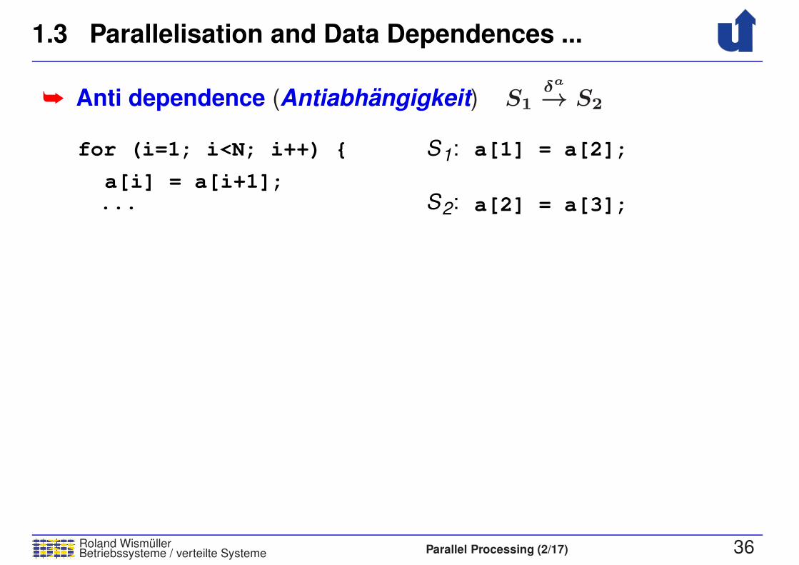
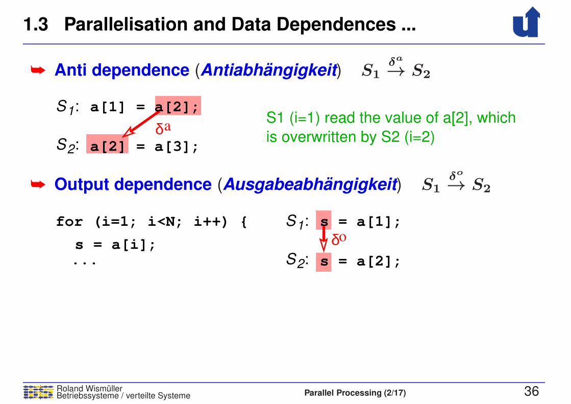
➥ Anti dependence (Antiabhangigkeit) S1δa
→ S2
for (i=1; i<N; i++) {
a[i] = a[i+1];...
1.3 Parallelisation and Data Dependences ...
Roland WismullerBetriebssysteme / verteilte Systeme Parallel Processing (2/17) 36
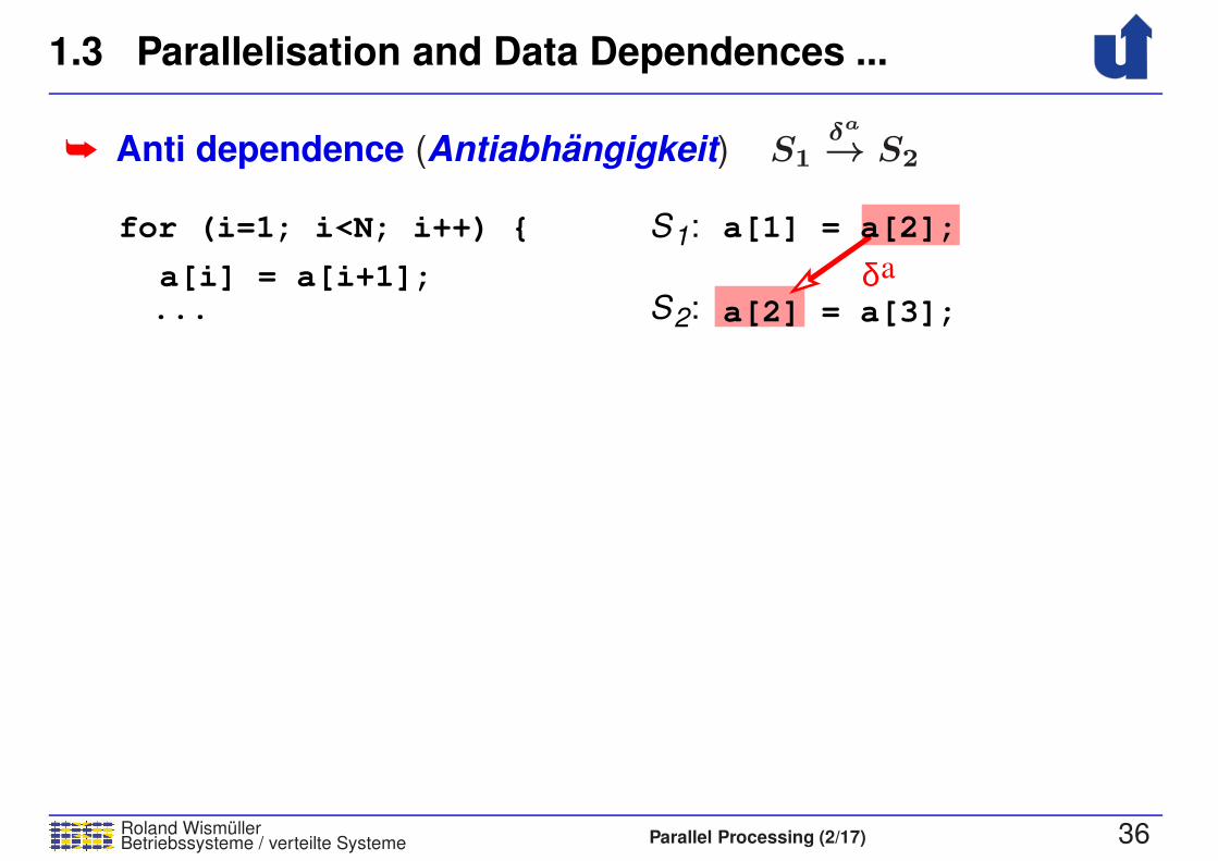
➥ Anti dependence (Antiabhangigkeit) S1δa
→ S2
S1:
S2:
a[1] = a[2];
a[2] = a[3];
for (i=1; i<N; i++) {
a[i] = a[i+1];...
1.3 Parallelisation and Data Dependences ...
Roland WismullerBetriebssysteme / verteilte Systeme Parallel Processing (2/17) 36
➥ Anti dependence (Antiabhangigkeit) S1δa
→ S2
δa
S1:
S2:
a[1] = a[2];
a[2] = a[3];
for (i=1; i<N; i++) {
a[i] = a[i+1];...

1.3 Parallelisation and Data Dependences ...
Roland WismullerBetriebssysteme / verteilte Systeme Parallel Processing (2/17) 36
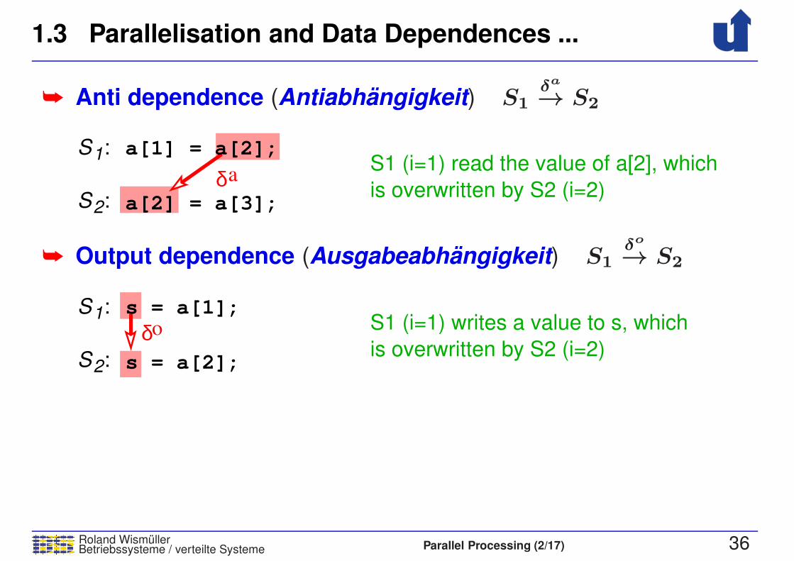
➥ Anti dependence (Antiabhangigkeit) S1δa
→ S2
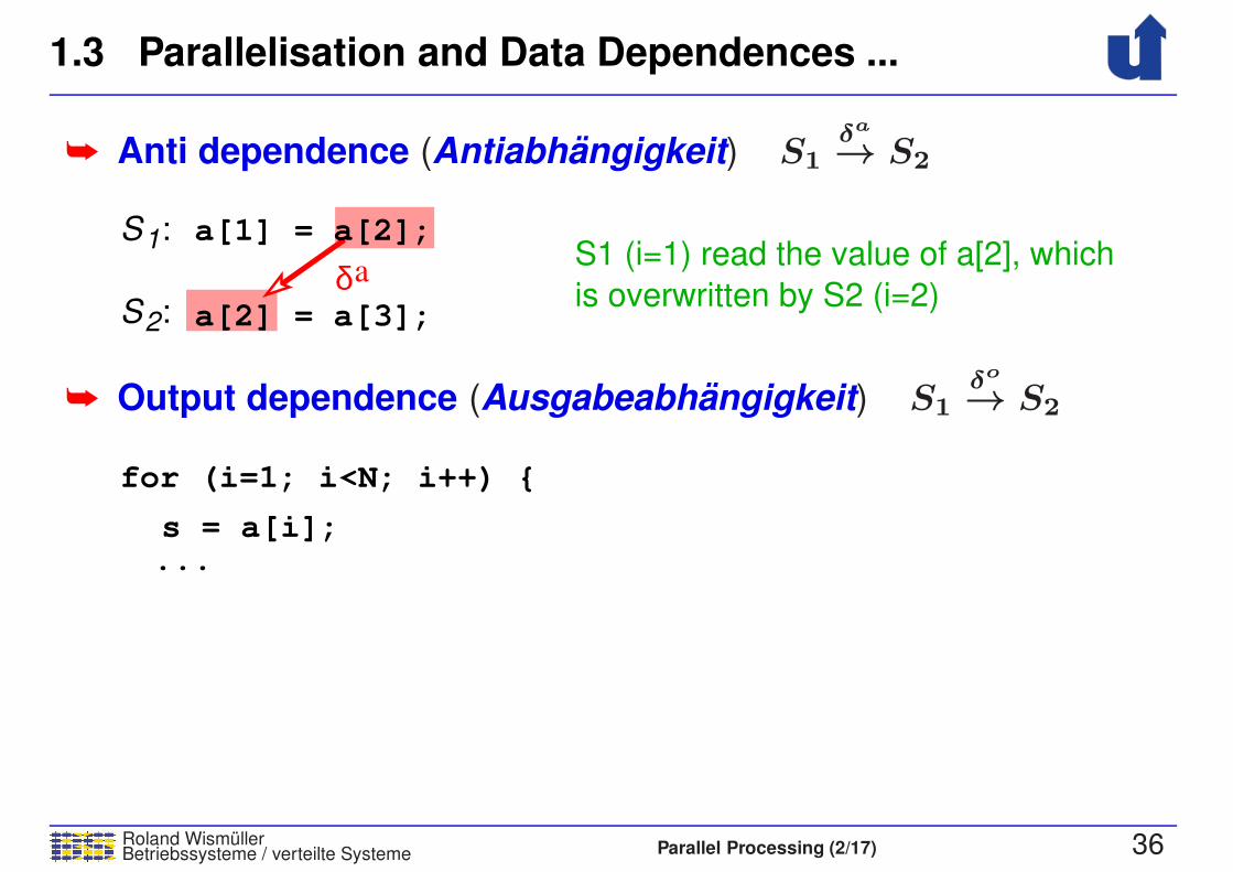
S1 (i=1) read the value of a[2], which
is overwritten by S2 (i=2)δa
S1:
S2:
a[1] = a[2];
a[2] = a[3];
1.3 Parallelisation and Data Dependences ...
Roland WismullerBetriebssysteme / verteilte Systeme Parallel Processing (2/17) 36
➥ Anti dependence (Antiabhangigkeit) S1δa
→ S2
S1 (i=1) read the value of a[2], which
is overwritten by S2 (i=2)δa
S1:
S2:
a[1] = a[2];
a[2] = a[3];
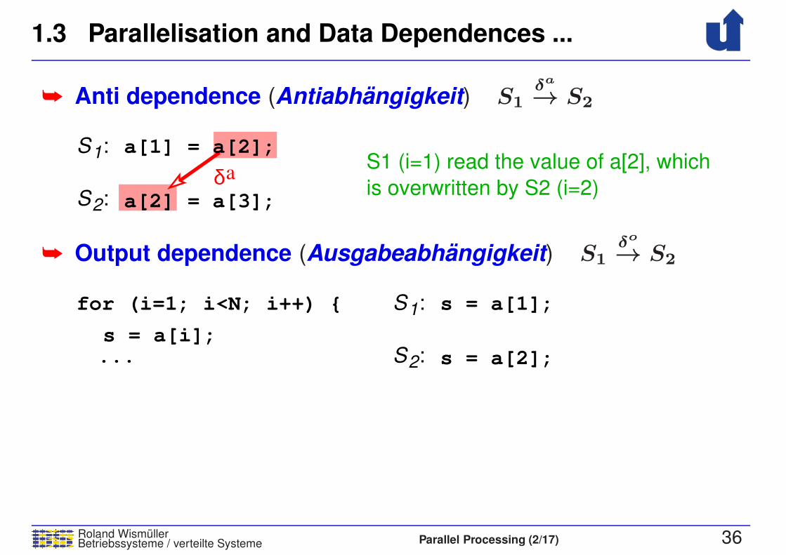
➥ Output dependence (Ausgabeabhangigkeit) S1δo
→ S2
for (i=1; i<N; i++) {
...s = a[i];
1.3 Parallelisation and Data Dependences ...
Roland WismullerBetriebssysteme / verteilte Systeme Parallel Processing (2/17) 36
➥ Anti dependence (Antiabhangigkeit) S1δa
→ S2
S1 (i=1) read the value of a[2], which
is overwritten by S2 (i=2)δa
S1:
S2:
a[1] = a[2];
a[2] = a[3];
➥ Output dependence (Ausgabeabhangigkeit) S1δo
→ S2
S1:
S2:
s = a[1];
s = a[2];
for (i=1; i<N; i++) {
...s = a[i];
1.3 Parallelisation and Data Dependences ...
Roland WismullerBetriebssysteme / verteilte Systeme Parallel Processing (2/17) 36
➥ Anti dependence (Antiabhangigkeit) S1δa
→ S2
S1 (i=1) read the value of a[2], which
is overwritten by S2 (i=2)δa
S1:
S2:
a[1] = a[2];
a[2] = a[3];
➥ Output dependence (Ausgabeabhangigkeit) S1δo
→ S2
oδS1:
S2:
s = a[1];
s = a[2];
for (i=1; i<N; i++) {
...s = a[i];
1.3 Parallelisation and Data Dependences ...
Roland WismullerBetriebssysteme / verteilte Systeme Parallel Processing (2/17) 36
➥ Anti dependence (Antiabhangigkeit) S1δa
→ S2
S1 (i=1) read the value of a[2], which
is overwritten by S2 (i=2)δa
S1:
S2:
a[1] = a[2];
a[2] = a[3];
➥ Output dependence (Ausgabeabhangigkeit) S1δo
→ S2
S1 (i=1) writes a value to s, which
is overwritten by S2 (i=2)oδ
S1:
S2:
s = a[1];
s = a[2];
➥ Anti and Output dependences can always be removed by
consistent renaming of variables

1.3 Parallelisation and Data Dependences ...
Roland WismullerBetriebssysteme / verteilte Systeme Parallel Processing (2/17) 37
Data dependences and synchronisation
➥ Two instructions S1 and S2 with a data dependence S1 → S2
can be distributed by different threads, if a correct
synchronisation is performed
➥ S2 must be executed after S1
➥ e.g., by using signal/wait or a message
➥ in the previous example:
y = a * (c−5);
x = b + 2 * a;
z = abs(x−y);

1.3 Parallelisation and Data Dependences ...
Roland WismullerBetriebssysteme / verteilte Systeme Parallel Processing (2/17) 37
Data dependences and synchronisation
➥ Two instructions S1 and S2 with a data dependence S1 → S2
can be distributed by different threads, if a correct
synchronisation is performed
➥ S2 must be executed after S1
➥ e.g., by using signal/wait or a message
➥ in the previous example:
Thread 1 Thread 2
wait(cond);y = a * (c−5);signal(cond);
x = b + 2 * a;
z = abs(x−y);
1.4 Parallel Computer Architectures
Roland WismullerBetriebssysteme / verteilte Systeme Parallel Processing (2/17) 38
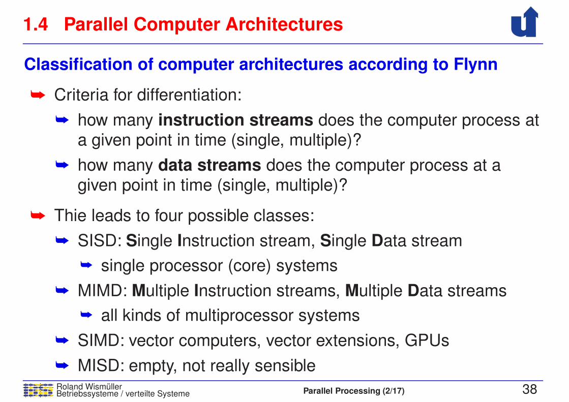
Classification of computer architectures according to Flynn
➥ Criteria for differentiation:
➥ how many instruction streams does the computer process ata given point in time (single, multiple)?
➥ how many data streams does the computer process at agiven point in time (single, multiple)?
➥ Thie leads to four possible classes:
➥ SISD: Single Instruction stream, Single Data stream
➥ single processor (core) systems
➥ MIMD: Multiple Instruction streams, Multiple Data streams
➥ all kinds of multiprocessor systems
➥ SIMD: vector computers, vector extensions, GPUs
➥ MISD: empty, not really sensible
1.4 Parallel Computer Architectures ...
Roland WismullerBetriebssysteme / verteilte Systeme Parallel Processing (2/17) 39
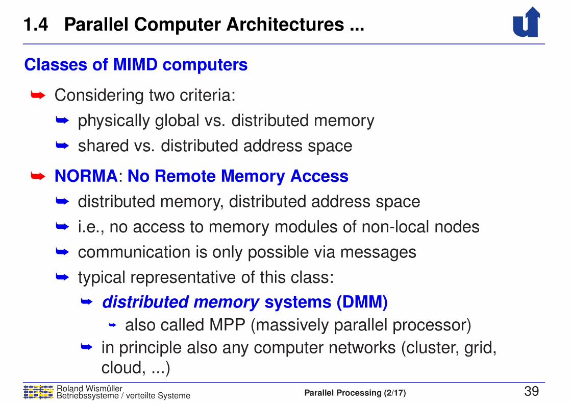
Classes of MIMD computers
➥ Considering two criteria:
➥ physically global vs. distributed memory
➥ shared vs. distributed address space
➥ NORMA: No Remote Memory Access
➥ distributed memory, distributed address space
➥ i.e., no access to memory modules of non-local nodes
➥ communication is only possible via messages
➥ typical representative of this class:
➥ distributed memory systems (DMM)➥ also called MPP (massively parallel processor)
➥ in principle also any computer networks (cluster, grid,cloud, ...)
1.4 Parallel Computer Architectures ...
Roland WismullerBetriebssysteme / verteilte Systeme Parallel Processing (2/17) 40
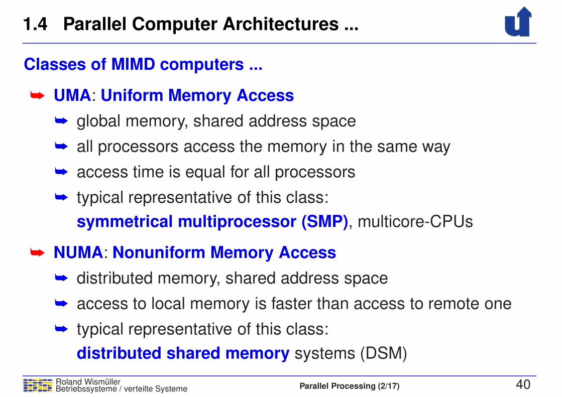
Classes of MIMD computers ...
➥ UMA: Uniform Memory Access
➥ global memory, shared address space
➥ all processors access the memory in the same way
➥ access time is equal for all processors
➥ typical representative of this class:
symmetrical multiprocessor (SMP), multicore-CPUs
➥ NUMA: Nonuniform Memory Access
➥ distributed memory, shared address space
➥ access to local memory is faster than access to remote one
➥ typical representative of this class:
distributed shared memory systems (DSM)
1.4 Parallel Computer Architectures ...
Roland WismullerBetriebssysteme / verteilte Systeme Parallel Processing (2/17) 41
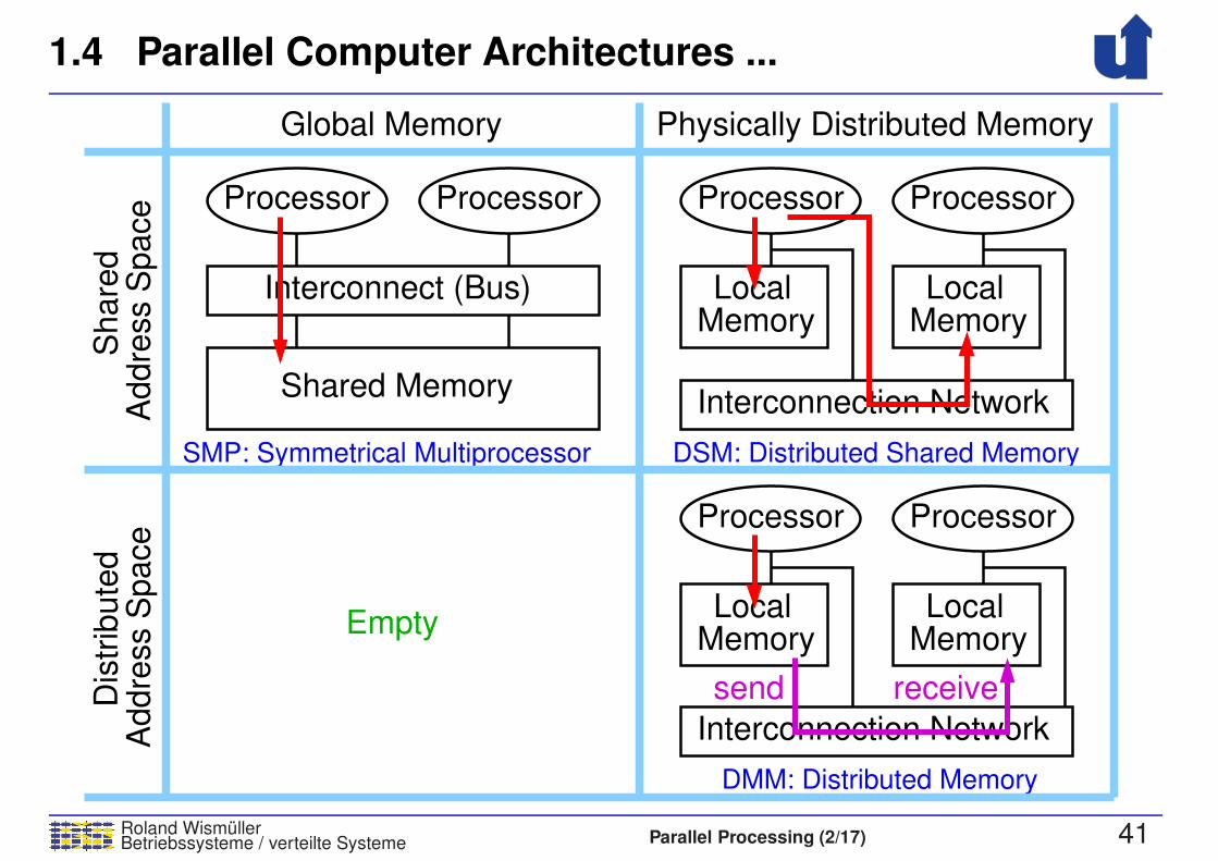
SMP: Symmetrical Multiprocessor DSM: Distributed Shared Memory
Interconnection Network
Interconnection Network
DMM: Distributed Memory
Processor Processor
Processor ProcessorProcessorProcessor
Shared Memory
MemoryLocal Local
Memory
LocalMemory
LocalMemory
Dis
trib
ute
dA
ddre
ss S
pace
Addre
ss S
pace
Share
dPhysically Distributed MemoryGlobal Memory
Interconnect (Bus)
Empty
send receive
1.4.1 MIMD: Message Passing Systems
Roland WismullerBetriebssysteme / verteilte Systeme Parallel Processing (2/17) 42
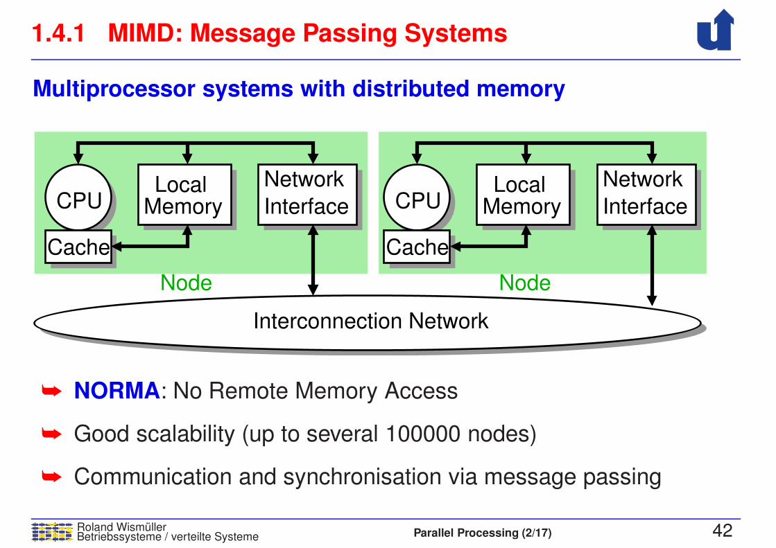
Multiprocessor systems with distributed memory
CPU
Cache
CPU
Cache
NetworkNetwork
Memory MemoryLocal Local
Node Node
Interface Interface
Interconnection Network
➥ NORMA: No Remote Memory Access
➥ Good scalability (up to several 100000 nodes)
➥ Communication and synchronisation via message passing

1.4.1 MIMD: Message Passing Systems ...
Roland WismullerBetriebssysteme / verteilte Systeme Parallel Processing (2/17) 43
Historical evolution
➥ In former times: proprietary hardware for nodes and network
➥ distinct node architecture (processor, network adapter, ...)
➥ often static interconnection networks with store and forward
➥ often distinct (mini) operating systems
➥ Today:
➥ cluster with standard components (PC server)
➥ often with high performance network (Infiniband, Myrinet, ...)
➥ often with SMP and/or vector computers as nodes
➥ for high performance computers
➥ dynamic (switched) interconnection networks
➥ standard operating systems (UNIX or Linux derivates)
1.4.1 MIMD: Message Passing Systems ...
Roland WismullerBetriebssysteme / verteilte Systeme Parallel Processing (2/17) 44
Properties
➥ No shared memory or addess areas
➥ Communication via exchange of messages
➥ application layer: libraries like e.g., MPI
➥ system layer: proprietary protocols or TCP/IP
➥ latency caused by software often much larger than hardware
latency (∼ 1− 50µs vs. ∼ 20− 100ns)
➥ In principle unlimited scalability
➥ z.B. BlueGene/Q (Sequoia): 98304 nodes, (1572864 cores)

1.4.1 MIMD: Message Passing Systems ...
Roland WismullerBetriebssysteme / verteilte Systeme Parallel Processing (2/17) 45
Properties ...
➥ Independent operating system on each node
➥ Often with shared file system
➥ e.g., parallel file system, connected to each node via a
(distinct) interconnection network
➥ or simply NFS (in small clusters)
➥ Usually no single system image
➥ user/administrator “sees” several computers
➥ Often no direct, interactive access to all nodes
➥ batch queueing systems assign nodes (only) on request to
parallel programs
➥ often exclusively: space sharing, partitioning
➥ often small fixed partition for login and interactiv use

1.4.2 MIMD: Shared Memory Systems
Roland WismullerBetriebssysteme / verteilte Systeme Parallel Processing (2/17) 46
Symmetrical multiprocessors (SMP)
CPU CPU CPU
Centralized
Memory
Shared
Cache Cache Cache
Interconnect (Bus)
MemoryModule
MemoryModule
➥ Global address space
➥ UMA: uniform memory
access
➥ Communication and
Synchronisation via
shared memory
➥ only feasible with few
processors (ca. 2 - 32)
1.4.2 MIMD: Shared Memory Systems ...
Roland WismullerBetriebssysteme / verteilte Systeme Parallel Processing (2/17) 47
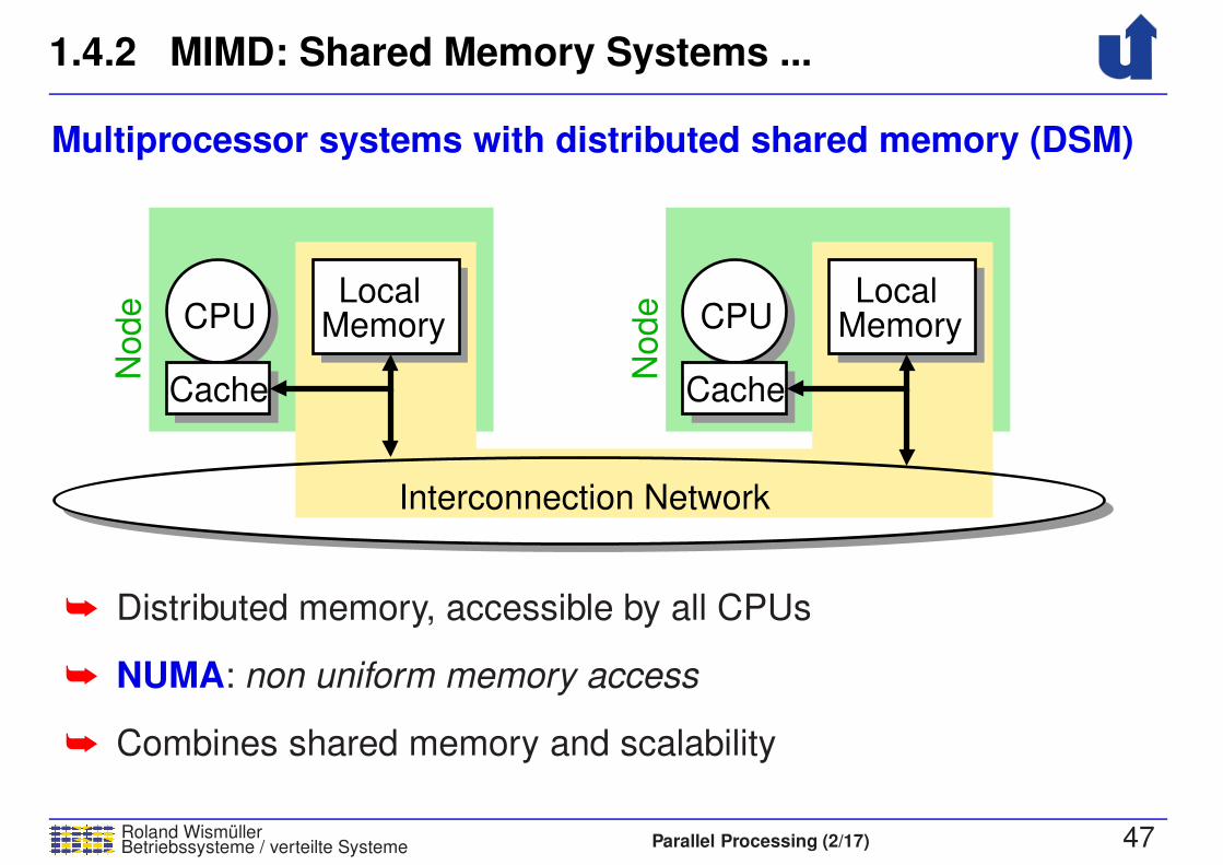
Multiprocessor systems with distributed shared memory (DSM)
CPU
Cache
CPU
Cache
Memory MemoryLocal Local
Node
Node
Interconnection Network
➥ Distributed memory, accessible by all CPUs
➥ NUMA: non uniform memory access
➥ Combines shared memory and scalability
1.4.2 MIMD: Shared Memory Systems ...
Roland WismullerBetriebssysteme / verteilte Systeme Parallel Processing (2/17) 48
Properties
➥ All Processors can access all resources in the same way
➥ but: different access times in NUMA architectures
➥ distribute the data such that most accesses are local
➥ Only one instance of the operating systems for the wholecomputer
➥ distributes processes/thread amongst the available processors
➥ all processors can execute operating system services in anequal way
➥ Single system image
➥ for user/administrator virtually no difference to a uniprocessorsystem
➥ Especially SMPs (UMA) only have limited scalability
1.4.2 MIMD: Shared Memory Systems ...
Roland WismullerBetriebssysteme / verteilte Systeme Parallel Processing (2/17) 49
Caches in shared memory systems
➥ Cache: fast intermediate storage, close to the CPU
➥ stores copies of the most recently used data from mainmemory
➥ when the data is in the cache: no access to main memory isnecessary
➥ access is 10-1000 times faster
➥ Cache are essential in multiprocessor systems
➥ otherwise memory and interconnection network quicklybecome a bottleneck
➥ exploiting the property of locality
➥ each process mostly works on “its own” data
➥ But: the existance of multiple copies of data cean lead toinconsistencies: cache coherence problem (☞ BS-1)
1.4.2 MIMD: Shared Memory Systems ...
Roland WismullerBetriebssysteme / verteilte Systeme Parallel Processing (2/17) 50
Enforcing cache coherency
➥ During a write access, all affected caches (= caches with copies)
must be notified
➥ caches invalidate or update the affected entry
➥ In UMA systems
➥ Bus as interconnection network: every access to main
memory is visible for everybody (broadcast)
➥ Caches “listen in” on the bus (bus snooping)
➥ (relatively) simple cache coherence protocols
➥ e.g., MESI protocol
➥ but: bad scalability, since the bus is a shared central resource
1.4.2 MIMD: Shared Memory Systems ...
Roland WismullerBetriebssysteme / verteilte Systeme Parallel Processing (2/17) 51
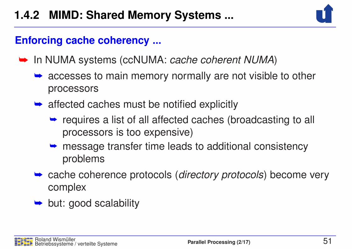
Enforcing cache coherency ...
➥ In NUMA systems (ccNUMA: cache coherent NUMA)
➥ accesses to main memory normally are not visible to other
processors
➥ affected caches must be notified explicitly
➥ requires a list of all affected caches (broadcasting to all
processors is too expensive)
➥ message transfer time leads to additional consistency
problems
➥ cache coherence protocols (directory protocols) become very
complex
➥ but: good scalability
1.4.2 MIMD: Shared Memory Systems ...
Roland WismullerBetriebssysteme / verteilte Systeme Parallel Processing (2/17) 52
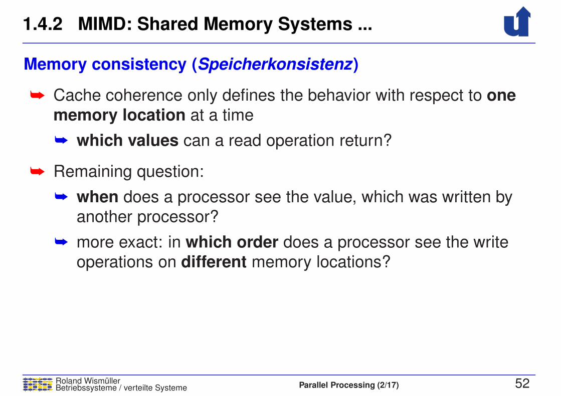
Memory consistency (Speicherkonsistenz)
➥ Cache coherence only defines the behavior with respect to onememory location at a time
➥ which values can a read operation return?
➥ Remaining question:
➥ when does a processor see the value, which was written by
another processor?
➥ more exact: in which order does a processor see the write
operations on different memory locations?
1.4.2 MIMD: Shared Memory Systems ...
Roland WismullerBetriebssysteme / verteilte Systeme Parallel Processing (2/17) 53
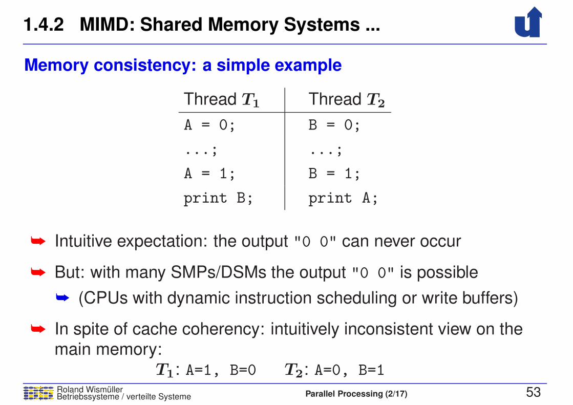
Memory consistency: a simple example
Thread T1 Thread T2
A = 0; B = 0;
...; ...;
A = 1; B = 1;
print B; print A;
➥ Intuitive expectation: the output "0 0" can never occur
➥ But: with many SMPs/DSMs the output "0 0" is possible
➥ (CPUs with dynamic instruction scheduling or write buffers)
➥ In spite of cache coherency: intuitively inconsistent view on the
main memory:T1: A=1, B=0 T2: A=0, B=1

1.4.2 MIMD: Shared Memory Systems ...
Roland WismullerBetriebssysteme / verteilte Systeme Parallel Processing (2/17) 54
Definition: sequential consistency
Sequential consistency is given, when the result of each execution of
a parallel program can also be produced by the following abstract
machine:
P2 Pn. . .P1
Main Memory
Processors execute
memory operations
in program order
The switch will be randomly switched
after each memory access
1.4.2 MIMD: Shared Memory Systems ...
Roland WismullerBetriebssysteme / verteilte Systeme Parallel Processing (2/17) 55
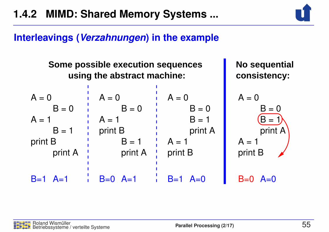
Interleavings (Verzahnungen) in the example
A = 0
B = 1
print A
print B
A = 0
B = 1
print A
A = 0
B = 0
print A
B = 1
A = 1
print B
print B
B = 0
A = 1
B = 0
A = 1
A = 0
B = 0
print A
print B
B = 1
A = 1
B=0
consistency:
B=1 A=1 B=0 A=1 B=1 A=0 A=0
No sequentialusing the abstract machine:
Some possible execution sequences
1.4.2 MIMD: Shared Memory Systems ...
Roland WismullerBetriebssysteme / verteilte Systeme Parallel Processing (2/17) 56
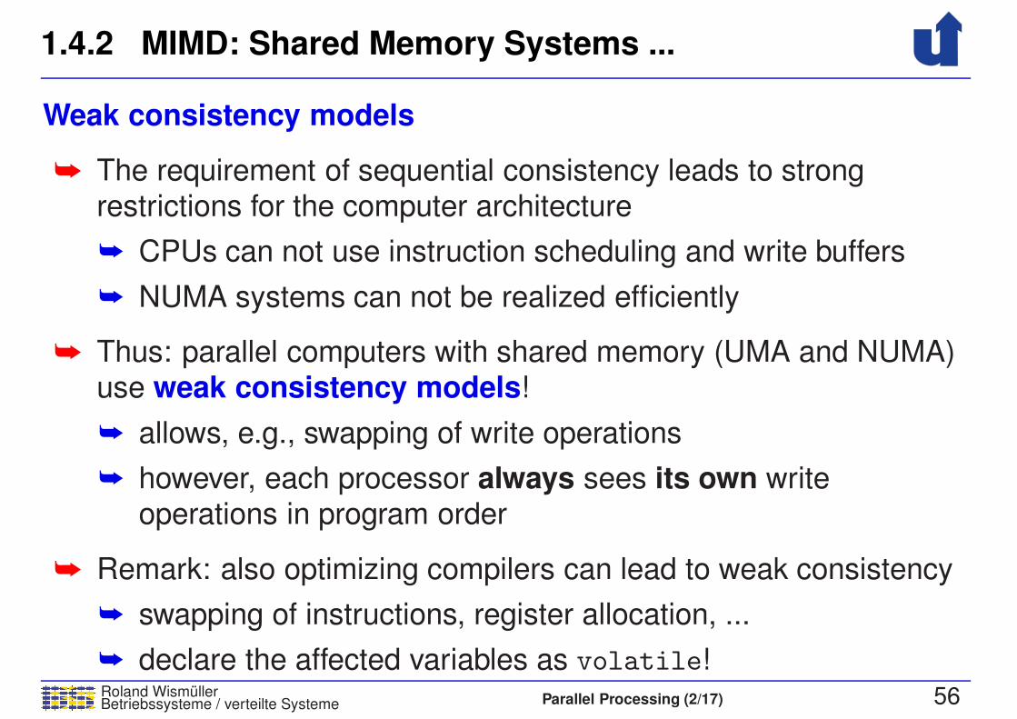
Weak consistency models
➥ The requirement of sequential consistency leads to strongrestrictions for the computer architecture
➥ CPUs can not use instruction scheduling and write buffers
➥ NUMA systems can not be realized efficiently
➥ Thus: parallel computers with shared memory (UMA and NUMA)use weak consistency models!
➥ allows, e.g., swapping of write operations
➥ however, each processor always sees its own writeoperations in program order
➥ Remark: also optimizing compilers can lead to weak consistency
➥ swapping of instructions, register allocation, ...
➥ declare the affected variables as volatile!
1.4.2 MIMD: Shared Memory Systems ...
Roland WismullerBetriebssysteme / verteilte Systeme Parallel Processing (2/17) 57
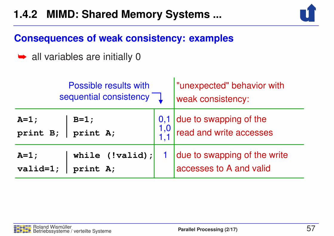
Consequences of weak consistency: examples
➥ all variables are initially 0
print A;
while (!valid);
valid=1;
A=1;
print A;print B;
B=1;A=1;
Possible results with
sequential consistency
accesses to A and valid
due to swapping of the write
read and write accesses
due to swapping of the
weak consistency:
"unexpected" behavior with
0,11,01,1
1

Roland WismullerBetriebssysteme / verteilte Systeme Parallel Processing (3/17) iv
Roland Wismuller
Universitat Siegen
Tel.: 0271/740-4050, Buro: H-B 8404
Stand: January 23, 2018
Parallel Processing
WS 2017/18
16.10.2017

1.4.2 MIMD: Shared Memory Systems ...
Roland WismullerBetriebssysteme / verteilte Systeme Parallel Processing (3/17) 58
Weak consistency models ...
➥ Memory consistency can (and must!) be enforced as needed,
using special instrcutions
➥ fence / memory barrier (Speicherbarriere)
➥ all previous memory operations are completed; subsequent
memory operations are started only after the barrier
➥ acquire and release
➥ acquire: subsequent memory operations are started only
after the acquire is finished
➥ release: all previous memory operations are completed
➥ pattern of use is equal to mutex locks
1.4.2 MIMD: Shared Memory Systems ...
Roland WismullerBetriebssysteme / verteilte Systeme Parallel Processing (3/17) 59
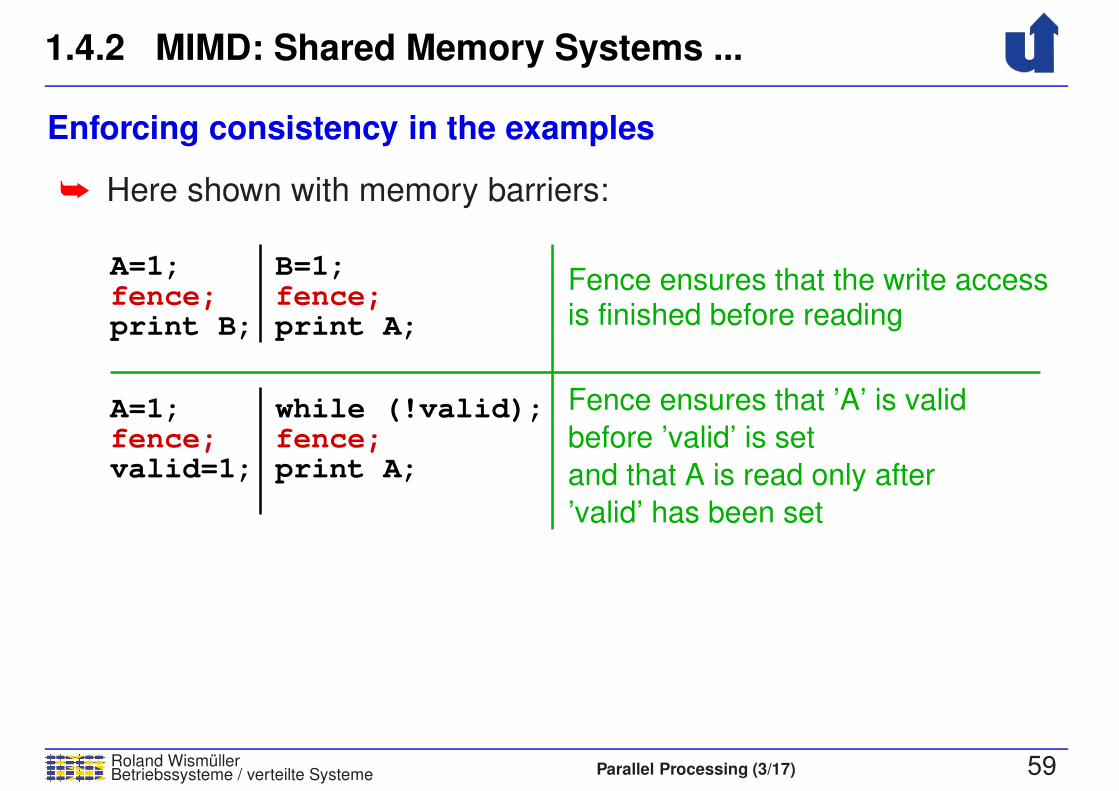
Enforcing consistency in the examples
➥ Here shown with memory barriers:
A=1;
print B;
A=1;
valid=1;
B=1;
print A;
while (!valid);
print A;
fence;
fence;
Fence ensures that the write accessis finished before reading
Fence ensures that ’A’ is valid
’valid’ has been set
before ’valid’ is set
and that A is read only after
fence;
fence;
1.4.3 SIMD
Roland WismullerBetriebssysteme / verteilte Systeme Parallel Processing (3/17) 60
➥ Only a single instruction stream, however, the instrcutions have
vectors as operands⇒ data parallelism
➥ Vector = one-dimensional array of numbers
➥ Variants:
➥ vector computers
➥ pipelined arithmetic units (vector uints) for the processing of
vectors
➥ SIMD extensions in processors (SSE)
➥ Intel: 128 Bit registers with, e.g., four 32 Bit float values
➥ graphics processors (GPUs)
➥ multiple streaming multiprocessors
➥ streaming multiprocessor contains several arithmetic units
(CUDA cores), which all execute the same instruction
1.4.3 SIMD ...
Roland WismullerBetriebssysteme / verteilte Systeme Parallel Processing (3/17) 61
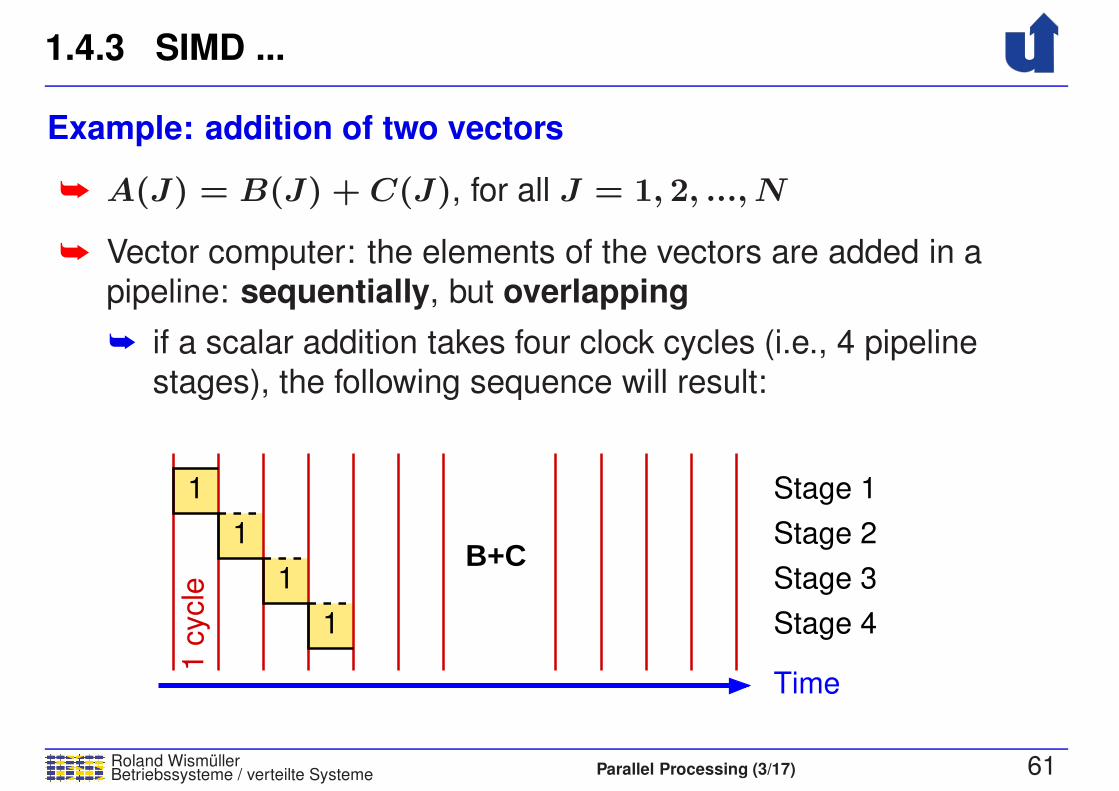
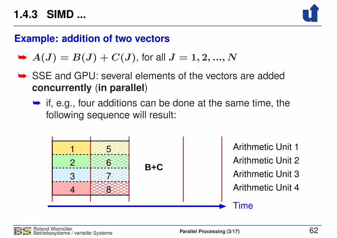
Example: addition of two vectors
➥ A(J) = B(J) + C(J), for all J = 1, 2, ..., N
➥ Vector computer: the elements of the vectors are added in a
pipeline: sequentially, but overlapping
➥ if a scalar addition takes four clock cycles (i.e., 4 pipeline
stages), the following sequence will result:
Time
Stage 4
Stage 3
Stage 2
Stage 1
1 c
ycle
1
1
1
1
B+C
1.4.3 SIMD ...
Roland WismullerBetriebssysteme / verteilte Systeme Parallel Processing (3/17) 61
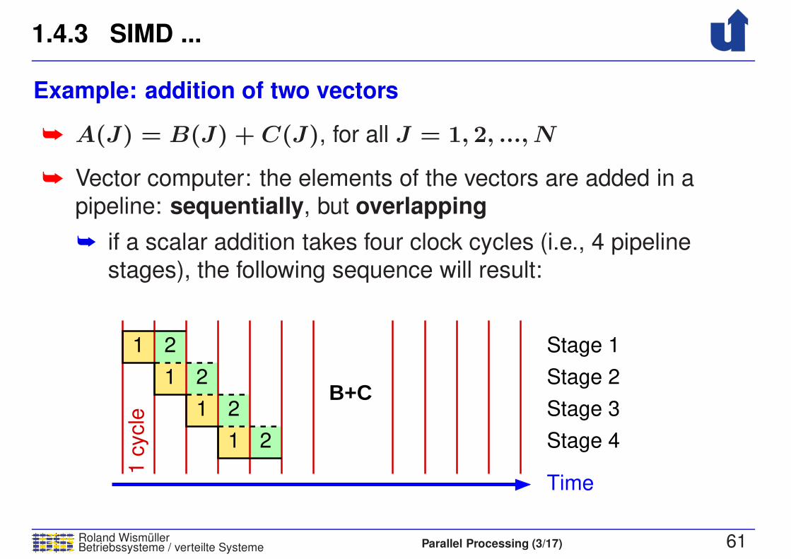
Example: addition of two vectors
➥ A(J) = B(J) + C(J), for all J = 1, 2, ..., N
➥ Vector computer: the elements of the vectors are added in a
pipeline: sequentially, but overlapping
➥ if a scalar addition takes four clock cycles (i.e., 4 pipeline
stages), the following sequence will result:
Time
Stage 4
Stage 3
Stage 2
Stage 1
1 c
ycle
1
1
1
1 2
2
2
2
B+C
1.4.3 SIMD ...
Roland WismullerBetriebssysteme / verteilte Systeme Parallel Processing (3/17) 61
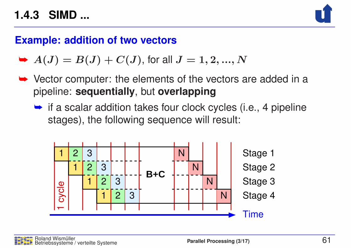
Example: addition of two vectors
➥ A(J) = B(J) + C(J), for all J = 1, 2, ..., N
➥ Vector computer: the elements of the vectors are added in a
pipeline: sequentially, but overlapping
➥ if a scalar addition takes four clock cycles (i.e., 4 pipeline
stages), the following sequence will result:
Time
Stage 4
Stage 3
Stage 2
Stage 1
1 c
ycle
1
1
1
1 2
2
2
2
3
3
N
N
N
N
3
3B+C
1.4.3 SIMD ...
Roland WismullerBetriebssysteme / verteilte Systeme Parallel Processing (3/17) 62
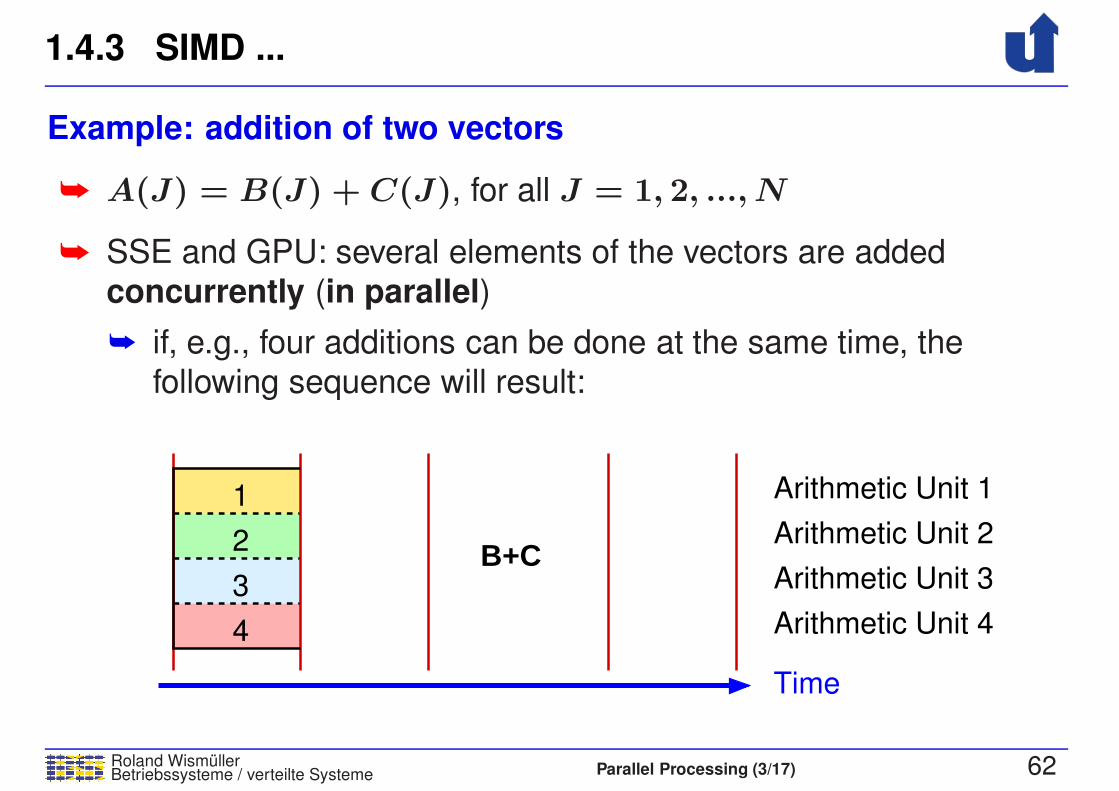
Example: addition of two vectors
➥ A(J) = B(J) + C(J), for all J = 1, 2, ..., N
➥ SSE and GPU: several elements of the vectors are added
concurrently (in parallel)
➥ if, e.g., four additions can be done at the same time, the
following sequence will result:
1
2
3
4
Time
Arithmetic Unit 1
Arithmetic Unit 2
Arithmetic Unit 3
Arithmetic Unit 4
B+C
1.4.3 SIMD ...
Roland WismullerBetriebssysteme / verteilte Systeme Parallel Processing (3/17) 62
Example: addition of two vectors
➥ A(J) = B(J) + C(J), for all J = 1, 2, ..., N
➥ SSE and GPU: several elements of the vectors are added
concurrently (in parallel)
➥ if, e.g., four additions can be done at the same time, the
following sequence will result:
������������
������������
����������������
����������������
����������������
����������������
������������
������������
5
6
7
8
1
2
3
4
Time
Arithmetic Unit 1
Arithmetic Unit 2
Arithmetic Unit 3
Arithmetic Unit 4
B+C
1.4.3 SIMD ...
Roland WismullerBetriebssysteme / verteilte Systeme Parallel Processing (3/17) 62
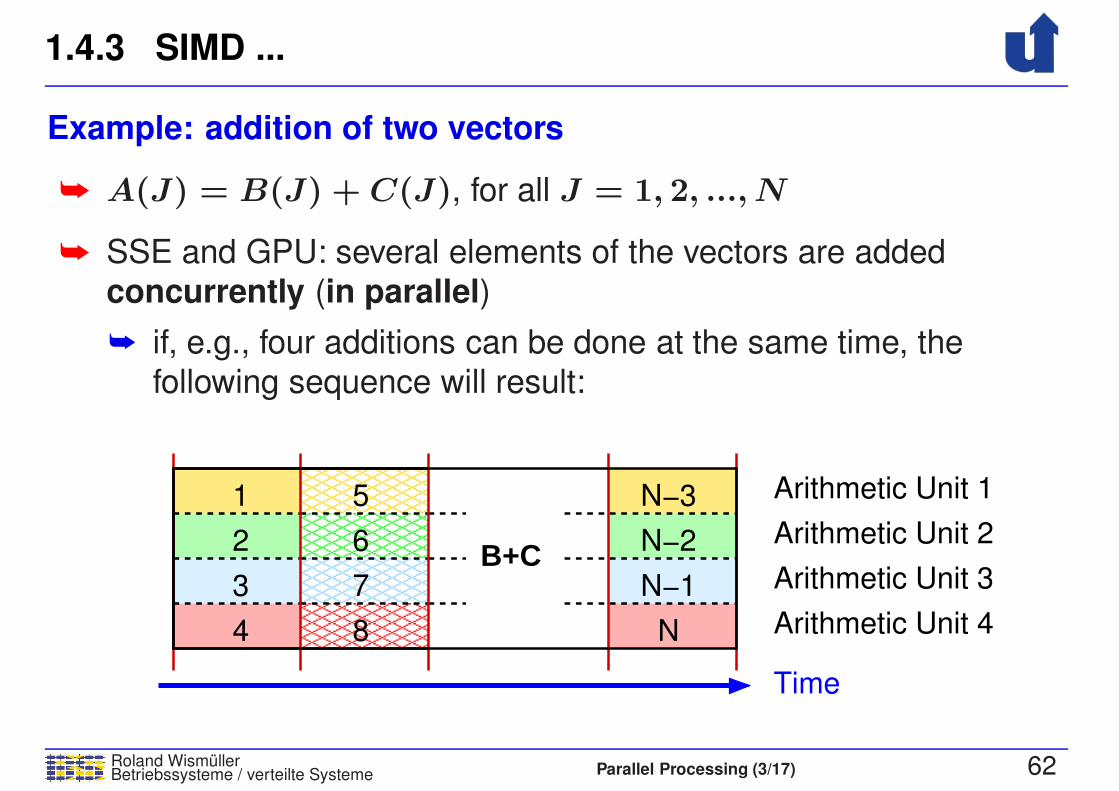
Example: addition of two vectors
➥ A(J) = B(J) + C(J), for all J = 1, 2, ..., N
➥ SSE and GPU: several elements of the vectors are added
concurrently (in parallel)
➥ if, e.g., four additions can be done at the same time, the
following sequence will result:
N−1
N−2
N−3
N
������������
������������
����������������
����������������
����������������
����������������
������������
������������
5
6
7
8
1
2
3
4
Time
Arithmetic Unit 1
Arithmetic Unit 2
Arithmetic Unit 3
Arithmetic Unit 4
B+C
1.4.3 SIMD ...
Roland WismullerBetriebssysteme / verteilte Systeme Parallel Processing (3/17) 63
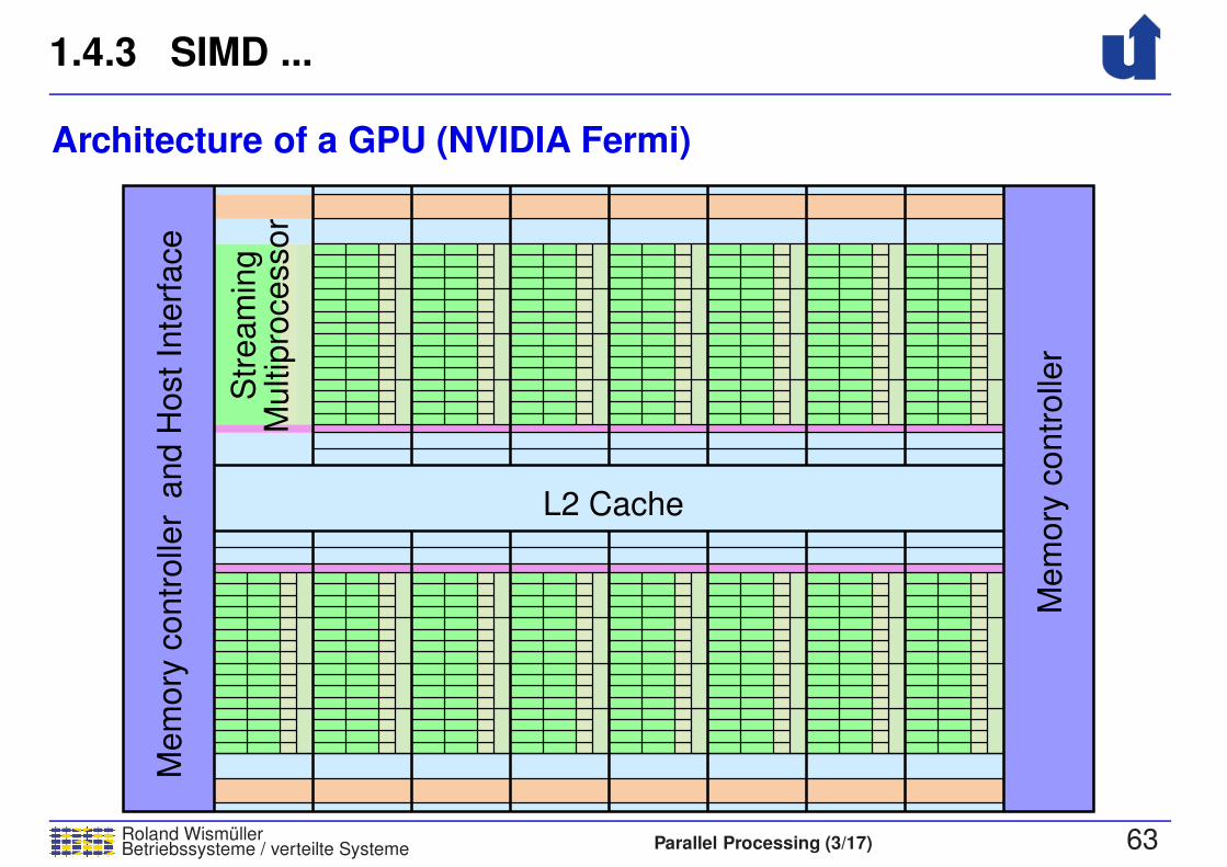
Architecture of a GPU (NVIDIA Fermi)M
em
ory
contr
olle
rand H
ost In
terf
ace
Mem
ory
contr
olle
r
Str
eam
ing
Multip
rocessor
L2 Cache

1.4.3 SIMD ...
Roland WismullerBetriebssysteme / verteilte Systeme Parallel Processing (3/17) 63
Architecture of a GPU (NVIDIA Fermi)M
em
ory
contr
olle
rand H
ost In
terf
ace
Mem
ory
contr
olle
r
Str
eam
ing
Multip
rocessor
L2 Cache
FP INT Core
Core
Core
Core
Core
Core
Core
LD/STLD/STLD/STLD/ST
LD/STLD/ST
LD/STLD/ST
LD/STLD/ST
LD/STLD/ST
LD/STLD/ST
LD/STLD/ST
Instruction Cache
Warp SchedulerWarp Scheduler
Dispatch Unit Dispatch Unit
Register File
Core Core
Core
Core
Core
Core
Core
Core
Core
SFU
SFU
SFU
SFU
Interconnect Network
Shared Memory / L1 Cache
Uniform Cache
1.4.3 SIMD ...
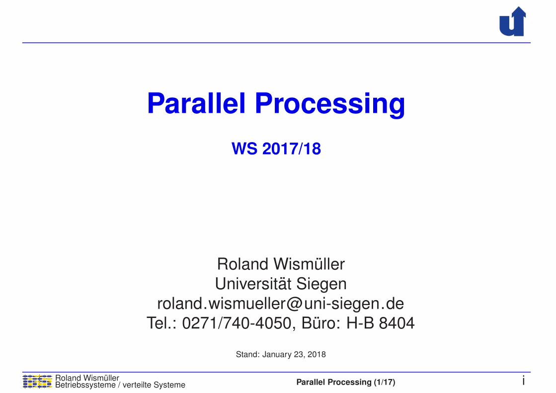
Roland WismullerBetriebssysteme / verteilte Systeme Parallel Processing (3/17) 64
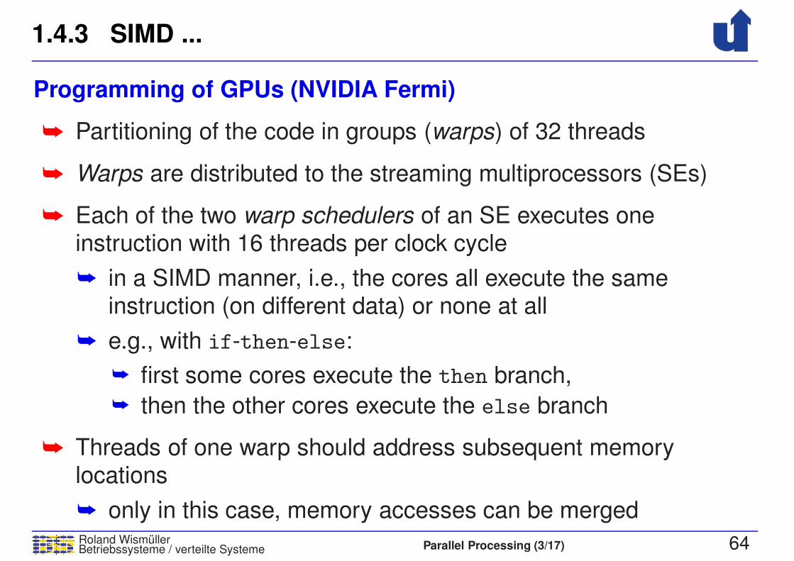
Programming of GPUs (NVIDIA Fermi)
➥ Partitioning of the code in groups (warps) of 32 threads
➥ Warps are distributed to the streaming multiprocessors (SEs)
➥ Each of the two warp schedulers of an SE executes oneinstruction with 16 threads per clock cycle
➥ in a SIMD manner, i.e., the cores all execute the sameinstruction (on different data) or none at all
➥ e.g., with if-then-else:
➥ first some cores execute the then branch,➥ then the other cores execute the else branch
➥ Threads of one warp should address subsequent memorylocations
➥ only in this case, memory accesses can be merged

1.4.4 High Performance Supercomputers
Roland WismullerBetriebssysteme / verteilte Systeme Parallel Processing (3/17) 65
Trends1993
1995
2000
2005
2010
2011
Source:
Top500 List
www.top500.org
SMP
SIMD
Uniprocessor
SMP Cluster
MPP and DSM
(PC) Cluster
1.4.4 High Performance Supercomputers ...
Roland WismullerBetriebssysteme / verteilte Systeme Parallel Processing (3/17) 66
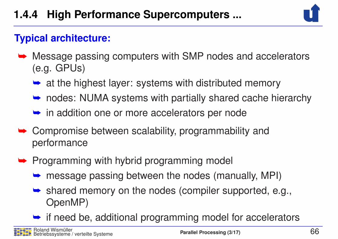
Typical architecture:
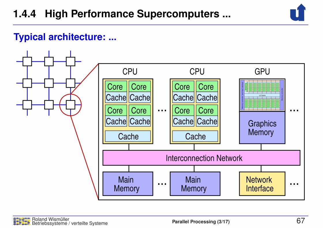
➥ Message passing computers with SMP nodes and accelerators(e.g. GPUs)
➥ at the highest layer: systems with distributed memory
➥ nodes: NUMA systems with partially shared cache hierarchy
➥ in addition one or more accelerators per node
➥ Compromise between scalability, programmability andperformance
➥ Programming with hybrid programming model
➥ message passing between the nodes (manually, MPI)
➥ shared memory on the nodes (compiler supported, e.g.,OpenMP)
➥ if need be, additional programming model for accelerators
1.4.4 High Performance Supercomputers ...
Roland WismullerBetriebssysteme / verteilte Systeme Parallel Processing (3/17) 67
Typical architecture: ...
Mem
ory
contr
oller
and H
ost In
terf
ace
Mem
ory
contr
oller
Str
eam
ing
Multip
rocessor
L2 Cache
Cache Cache
...
...
...
...Memory
MainMemory
Main
Core
Cache
Core
Cache
Core
Cache
Core
Cache
Core
Cache
Core
Cache
Core
Cache
Core
Cache
GPU
Graphics
CPU CPU
Interconnection Network
Memory
NetworkInterface
1.5 Parallel Programming Models
Roland WismullerBetriebssysteme / verteilte Systeme Parallel Processing (3/17) 68
In the followig, we discuss:
➥ Shared memory
➥ Message passing
➥ Distributed objects
➥ Data parallel languages
➥ The list is not complete (e.g., data flow models, PGAS)
1.5.1 Shared Memory
Roland WismullerBetriebssysteme / verteilte Systeme Parallel Processing (3/17) 69
➥ Light weight processes (threads) share a common virtual addressspace
➥ The “more simple” parallel programming model
➥ all threads have access to all data
➥ also good theoretical foundation (PRAM model)
➥ Mostly with shared memory computers
➥ however also implementable on distributed memory computers(with large performance panalty)
➥ shared virtual memory (SVM)
➥ Examples:
➥ PThreads, Java Threads
➥ Intel Threading Building Blocks (TBB)
➥ OpenMP (☞ 2.3)
1.5.1 Shared Memory ...
Roland WismullerBetriebssysteme / verteilte Systeme Parallel Processing (3/17) 70
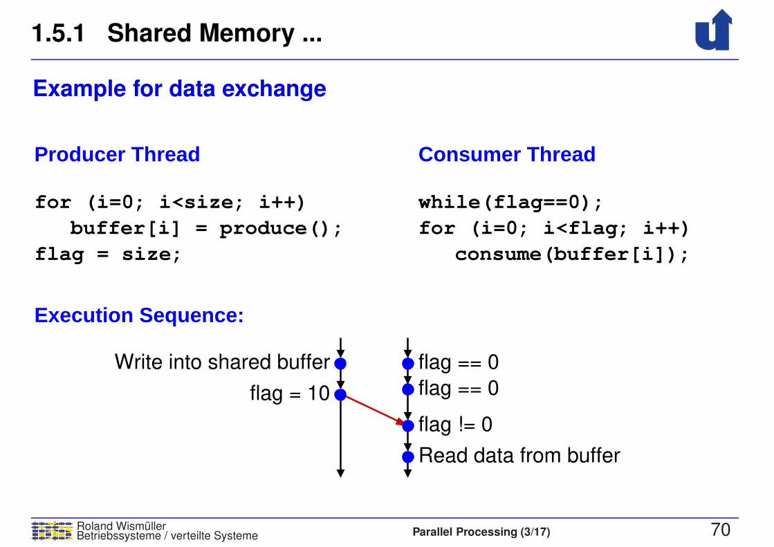
Example for data exchange
for (i=0; i<size; i++)
flag = size;
buffer[i] = produce();
Execution Sequence:
Producer Thread
while(flag==0);
for (i=0; i<flag; i++)
consume(buffer[i]);
Consumer Thread
flag != 0
flag == 0
flag == 0flag = 10
Write into shared buffer
Read data from buffer
1.5.2 Message Passing
Roland WismullerBetriebssysteme / verteilte Systeme Parallel Processing (3/17) 71
➥ Processes with separate address spaces
➥ Library routines for sending and receiving messages
➥ (informal) standard for parallel programming:
MPI (Message Passing Interface, ☞ 3.2)
➥ Mostly with distributed memory computers
➥ but also well usable with shared memory computers
➥ The “more complicated” parallel programming model
➥ explicit data distribution / explicit data transfer
➥ typically no compiler and/or language support
➥ parallelisation is done completely manually
1.5.2 Message Passing ...
Roland WismullerBetriebssysteme / verteilte Systeme Parallel Processing (3/17) 72
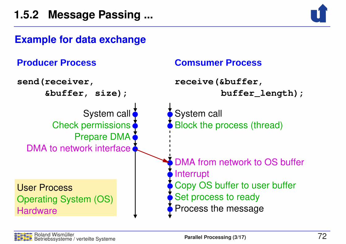
Example for data exchange
receive(&buffer,
buffer_length);&buffer, size);
System call
Block the process (thread)
Copy OS buffer to user buffer
Interrupt
DMA from network to OS buffer
Set process to ready
Process the message
send(receiver,
DMA to network interface
Prepare DMA
Check permissions
System call
Producer Process Comsumer Process
User Process
Hardware
Operating System (OS)

1.5.3 Distributed Objects
Roland WismullerBetriebssysteme / verteilte Systeme Parallel Processing (3/17) 73
➥ Basis: (purely) object oriented programming
➥ access to data only via method calls
➥ Then: objects can be distributed to different address spaces
(computers)
➥ at object creation: additional specification of a node
➥ object reference then also identifies this node
➥ method calls via RPC mechanism
➥ e.g., Remote Method Invocation (RMI) in Java
➥ more about this: lecture “Verteilte Systeme”
➥ Distributed objects alone do not yet enable parallel processing
➥ additional concepts / extensions are necessary
➥ e.g., threads, asynchronous RPC, futures
1.5.4 Data Parallel Languages
Roland WismullerBetriebssysteme / verteilte Systeme Parallel Processing (3/17) 74
➥ Goal: support for data parallelism
➥ Sequential code is amended with compiler directives
➥ Specification, how to distribute data structures (typically
arrays) to processors
➥ Compiler automatically generates code for synchronisation or
communication, resprctively
➥ operations are executed on the processor that “possesses” the
result variable (owner computes rule)
➥ Example: HPF (High Performance Fortran)
➥ Despite easy programming not really successful
➥ only suited for a limited class of applications
➥ good performance requres a lot of manual optimization

1.5.4 Data Parallel Languages ...
Roland WismullerBetriebssysteme / verteilte Systeme Parallel Processing (3/17) 75
Example for HPF
!HPF$ ALIGN B(:,:) WITH A(:,:)
REAL A(N,N), B(N,N)
!HPF$ DISTRIBUTE A(BLOCK,*)
DO I = 1, N
DO J = 1, N
A(I,J) = A(I,J) + B(J,I)
END DO
END DO
Distribution with 4 processors:
A B
➥ Processor 0 executes computations for I = 1 .. N/4
➥ Problem in this example: a lot of communication is required
➥ B should be distributed in a different way

1.5.4 Data Parallel Languages ...
Roland WismullerBetriebssysteme / verteilte Systeme Parallel Processing (3/17) 75
Example for HPF
!HPF$ ALIGN B(j,i) WITH A(i,j)
REAL A(N,N), B(N,N)
!HPF$ DISTRIBUTE A(BLOCK,*)
DO I = 1, N
DO J = 1, N
A(I,J) = A(I,J) + B(J,I)
END DO
END DO
Distribution with 4 processors:
A B
➥ Processor 0 executes computations for I = 1 .. N/4
➥ No communication is required any more
➥ but B must be redistributed, if neccessary
1.6 Focus of this Lecture
Roland WismullerBetriebssysteme / verteilte Systeme Parallel Processing (3/17) 76
➥ Explicit parallelism
➥ Process and block level
➥ Coarse and mid grained parallelism
➥ MIMD computers (with SIMD extensions)
➥ Programming models:
➥ shared memory
➥ message passing
1.7 A Design Process for Parallel Programs
Roland WismullerBetriebssysteme / verteilte Systeme Parallel Processing (3/17) 77
Four design steps:
1. Partitioning
➥ split the problem into many tasks
2. Communication
➥ specify the information flow between the tasks
➥ determine the communication structure
3. Agglomeration
➥ evaluate the performance (tasks, communication structure)
➥ if need be, aggregate tasks into larger tasks
4. Mapping
➥ map the tasks to processors
(See Foster: Designing and Building Parallel Programs, Ch. 2)

1.7 A Design Process for Parallel Programs ...
Roland WismullerBetriebssysteme / verteilte Systeme Parallel Processing (3/17) 78
Split the problem
of Tasks
Merging
between tasks
Data exchange
tasks as possible
in as many small
Mapping to
Processors
Degree ofparallelism
Goal: s
cala
bility
perfo
rmance
Goal: lo
cality
Problem
Communication
Agglomeration
Partitioning
Mapping
1.7.1 Partitioning
Roland WismullerBetriebssysteme / verteilte Systeme Parallel Processing (3/17) 79
➥ Goal: split the problem into as many small tasks as possible
Data partitioning (data parallelism)
➥ Tasks specify identical computaions for a part of the data
➥ In general, high degree of parallelism is possible
➥ We can distribute:
➥ input data
➥ output data
➥ intermediate data
➥ In some cases: recursive distribution (divide and conquer )
➥ Special case: distribution of search space in search problems
1.7.1 Partitioning ...
Roland WismullerBetriebssysteme / verteilte Systeme Parallel Processing (3/17) 80
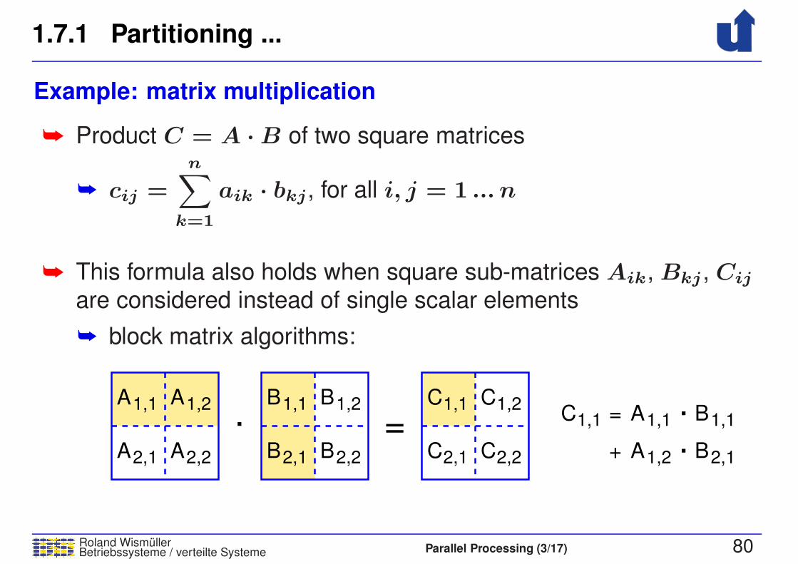
Example: matrix multiplication
➥ Product C = A ·B of two square matrices
➥ cij =n∑
k=1
aik · bkj, for all i, j = 1 ... n
➥ This formula also holds when square sub-matrices Aik, Bkj , Cij
are considered instead of single scalar elements
➥ block matrix algorithms:
. = .+ .
C1,1B1,1
B2,1
A1,1 B1,1
A1,2 B2,1
C1,1A1,1 A1,2
AA2,1 2,2
=C
CC2,1 2,2
1,2B
B2,2
1,2

1.7.1 Partitioning ...
Roland WismullerBetriebssysteme / verteilte Systeme Parallel Processing (3/17) 81
Example: matrix multiplication ...
➥ Distribution of output data: each task computes a sub-matrix of C
➥ E.g., distribution of C into four sub-matrices
(
A1,1 A1,2
A2,1 A2,2
)
·(
B1,1 B1,2
B2,1 B2,2
)
→(
C1,1 C1,2
C2,1 C2,2
)
➥ Results in four independent tasks:
1. C1,1 = A1,1 ·B1,1 +A1,2 · B2,1
2. C1,2 = A1,1 ·B1,2 +A1,2 · B2,2
3. C2,1 = A2,1 ·B1,1 +A2,2 · B2,1
4. C2,2 = A2,1 ·B1,2 +A2,2 · B2,2
1.7.1 Partitioning ...
Roland WismullerBetriebssysteme / verteilte Systeme Parallel Processing (3/17) 82
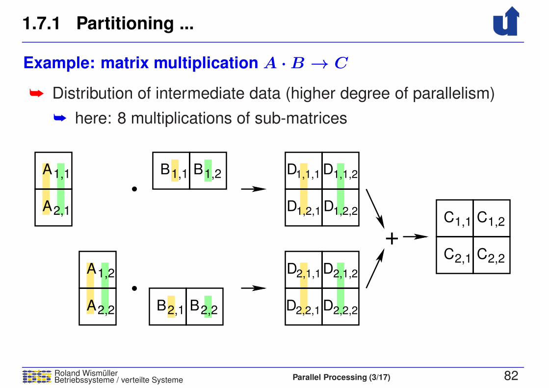
Example: matrix multiplication A ·B → C
➥ Distribution of intermediate data (higher degree of parallelism)
➥ here: 8 multiplications of sub-matrices
A1,1
A2,1
A1,2
A2,2
B1,1 B1,2
B2,1 B2,2
D D
DD
1,1,1
1,2,21,2,1
D
D D
D2,1,1 2,1,2
2,2,22,2,1
1,1,2
C1,1 C1,2
C2,1 C2,2
+

1.7.1 Partitioning ...
Roland WismullerBetriebssysteme / verteilte Systeme Parallel Processing (3/17) 83
Example: minimum of an array
➥ Distribution of input data
➥ each threads computates its local minimum
➥ afterwards: computation of the global minimum
23
144 53
8 39 8 6 54 8 9 4 8 7 5 7 8 8

1.7.1 Partitioning ...
Roland WismullerBetriebssysteme / verteilte Systeme Parallel Processing (3/17) 84
Example: sliding puzzle (partitioning of search space)
Finished!
solution:Found a
1 2 3 4
5 6
7
8
9 10 11
12131415
1 2 4
5 6
7
8
9 10 11
1213 1415
3
1 2 3 4
5
7
8
9 10 11
1213 1415
6
1 2 3 4
5 6
79 10 11
1213 1415
8
1 2 3 4
5 6 8
9 10 11
1213 1415
7
Task 1 Task 2 Task 3 Task 4
Partitioning of
1 2 3 4
8765
9 10 12
151413
11
the seach space
Goal: find a sequence of
sorted configuration
moves, which leads to a
1.7.1 Partitioning ...
Roland WismullerBetriebssysteme / verteilte Systeme Parallel Processing (3/17) 85
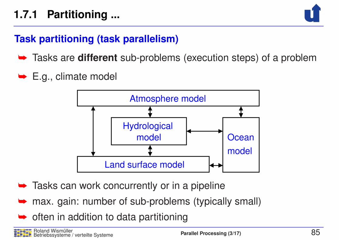
Task partitioning (task parallelism)
➥ Tasks are different sub-problems (execution steps) of a problem
➥ E.g., climate model
model
Oceanmodel
Atmosphere model
Hydrological
Land surface model
➥ Tasks can work concurrently or in a pipeline
➥ max. gain: number of sub-problems (typically small)
➥ often in addition to data partitioning

1.7.2 Communication
Roland WismullerBetriebssysteme / verteilte Systeme Parallel Processing (3/17) 86
➥ Two step approach
➥ definition of the communication structure
➥ who must exchange data with whom?
➥ sometimes complex, when using data partitioning
➥ often simple, when using task partitioning
➥ definition of the messages to be sent
➥ which data must be exchanges when?
➥ taking data dependences into account

1.7.2 Communication ...
Roland WismullerBetriebssysteme / verteilte Systeme Parallel Processing (3/17) 87
Different communication patterns:
➥ Local vs. global communication
➥ lokal: task communicates only with a small set of other tasks(its “neighbors”)
➥ global: task communicates with many/all other tasks
➥ Structured vs. unstructured communication
➥ structured: regular structure, e.g., grid, tree
➥ Static vs. dynamic communication
➥ dynamic: communication structure is changing duringrun-time, depending on computed data
➥ Synchronous vs. asynchronous communication
➥ asynchronous: the task owning the data does not know, whenother tasks need to access it
1.7.2 Communication ...
Roland WismullerBetriebssysteme / verteilte Systeme Parallel Processing (3/17) 88
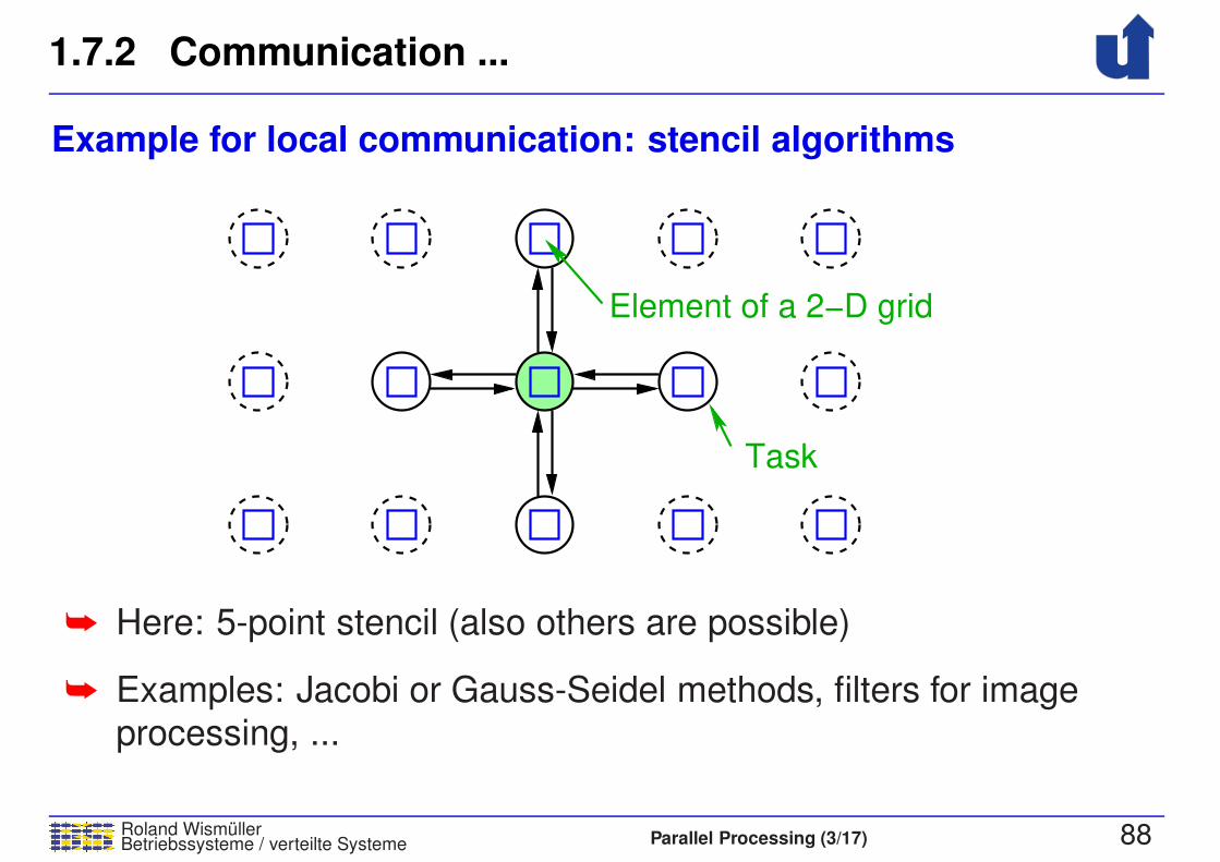
Example for local communication: stencil algorithms
Element of a 2−D grid
Task
➥ Here: 5-point stencil (also others are possible)
➥ Examples: Jacobi or Gauss-Seidel methods, filters for image
processing, ...
1.7.2 Communication ...
Roland WismullerBetriebssysteme / verteilte Systeme Parallel Processing (3/17) 89
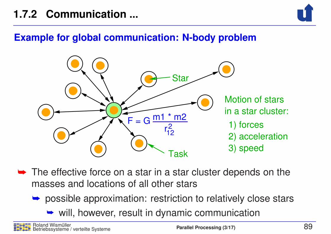
Example for global communication: N-body problem
Task
F = G m1 * m2
r212
Star
in a star cluster:
Motion of stars
1) forces
2) acceleration
3) speed
➥ The effective force on a star in a star cluster depends on themasses and locations of all other stars
➥ possible approximation: restriction to relatively close stars
➥ will, however, result in dynamic communication

Roland WismullerBetriebssysteme / verteilte Systeme Parallel Processing (4/17) v
Roland Wismuller
Universitat Siegen
Tel.: 0271/740-4050, Buro: H-B 8404
Stand: January 23, 2018
Parallel Processing
WS 2017/18
19.10.2017
1.7.2 Communication ...
Roland WismullerBetriebssysteme / verteilte Systeme Parallel Processing (4/17) 90
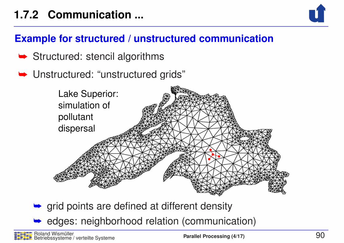
Example for structured / unstructured communication
➥ Structured: stencil algorithms
➥ Unstructured: “unstructured grids”
Lake Superior:
simulation of
pollutant
dispersal
➥ grid points are defined at different density
➥ edges: neighborhood relation (communication)
1.7.3 Agglomeration
Roland WismullerBetriebssysteme / verteilte Systeme Parallel Processing (4/17) 91
➥ So far: abstract parallel algorithms
➥ Now: concrete formulation for real computers
➥ limited number of processors
➥ costs for communication, process creation, process switching,
...
➥ Goals:
➥ reducing the communication costs
➥ aggregation of tasks
➥ replication of data and/or computation
➥ retaining the flexibility
➥ sufficently fine-grained parallelism for mapping phase
1.7.4 Mapping
Roland WismullerBetriebssysteme / verteilte Systeme Parallel Processing (4/17) 92
➥ Task: assignment of tasks to available processors
➥ Goal: minimizing the execution time
➥ Two (conflicting) strategies:
➥ map concurrently executable tasks to different processors
➥ high degree of parallelism
➥ map communicating tasks to the same processor
➥ higher locality (less communication)
➥ Constraint: load balancing
➥ (roughly) the same computing effort for each processor
➥ The mapping problem is NP complete
1.7.4 Mapping ...
Roland WismullerBetriebssysteme / verteilte Systeme Parallel Processing (4/17) 93
Variants of mapping techniques
➥ Static mapping
➥ fixed assignment of tasks to processors when program isstarted
➥ for algorithms on arrays or Cartesian grids:
➥ often manually, e.g., block wise or cyclic distribution
➥ for unstructured grids:
➥ graph partitioning algorithms, e.g., greedy, recursivecoordinate bisection, recursive spectral bisection, ...
➥ Dynamic mapping (dynamic load balancing)
➥ assignment of tasks to processors at runtime
➥ variants:➥ tasks stay on their processor until their execution ends
➥ task migration is possible during runtime

1.7.4 Mapping ...
Roland WismullerBetriebssysteme / verteilte Systeme Parallel Processing (4/17) 94
Example: static mapping with unstructured grid
➥ (Roughly) the same number of grid points per processor
➥ Short boundaries: small amount of communication
1.8 Organisation Forms for Parallel Programs
Roland WismullerBetriebssysteme / verteilte Systeme Parallel Processing (4/17) 95
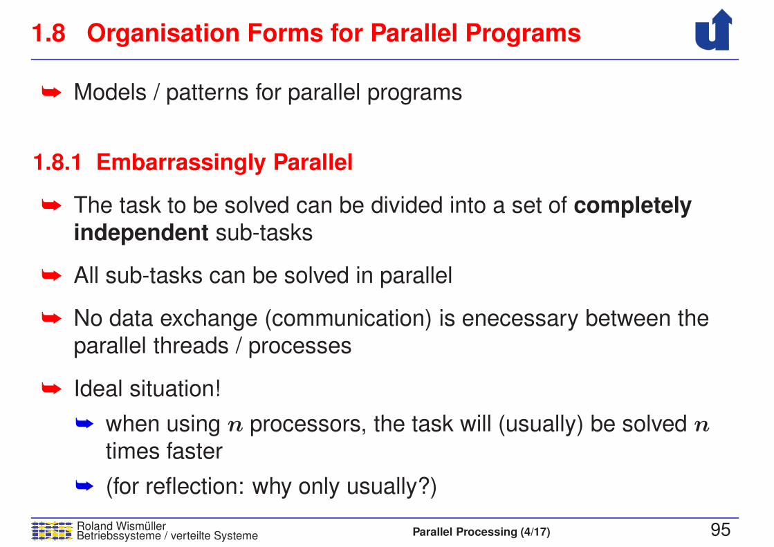
➥ Models / patterns for parallel programs
1.8.1 Embarrassingly Parallel
➥ The task to be solved can be divided into a set of completelyindependent sub-tasks
➥ All sub-tasks can be solved in parallel
➥ No data exchange (communication) is enecessary between the
parallel threads / processes
➥ Ideal situation!
➥ when using n processors, the task will (usually) be solved ntimes faster
➥ (for reflection: why only usually?)
1.8.1 Embarrassingly Parallel ...
Roland WismullerBetriebssysteme / verteilte Systeme Parallel Processing (4/17) 96
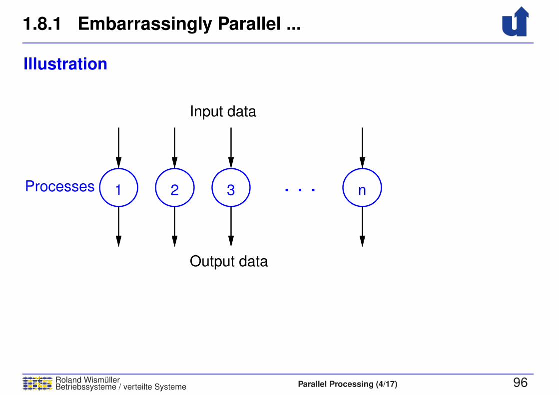
Illustration
Input data
Output data
Processes . . .1 2 3 n
1.8.1 Embarrassingly Parallel ...
Roland WismullerBetriebssysteme / verteilte Systeme Parallel Processing (4/17) 97
Examples for embarrassingly parallel problems
➥ Computation of animations
➥ animated cartoons, zoom into the Mandelbrot Set, ...
➥ each image (frame) can be computed independently
➥ Parameter studies
➥ multiple / many simulations with different input parameters
➥ e.g., weather forecast with provision for measurement errors,
computational fluid dynamics for optimizing an airfoil, ...

1.8 Organisation Forms for Parallel Programs ...
Roland WismullerBetriebssysteme / verteilte Systeme Parallel Processing (4/17) 98
1.8.2 Manager/Worker Model (Master/Slave Model)
➥ A manager process creates tasks
and assigns them to worker
processes
➥ several managers are possible,
too
➥ a hierarchy is possible, too: a
worker can itself be the manager
of own workers
S1 S2 S3 S4
Manager
Workers
➥ The manager (or sometimes also the workers) can createadditional tasks, while the workers are working
➥ The manager can becom a bottleneck
➥ The manager should be able to receive the results asynchronously(non blocking)

1.8.2 Manager/Worker Model (Master/Slave Model) ...
Roland WismullerBetriebssysteme / verteilte Systeme Parallel Processing (4/17) 99
Typical application
➥ Often only a part of a task can be parallelised in an optimal way
➥ In the easiest case, the following flow will result:
. . .(Slaves)
Workers
Distribute tasks (input)
1 2 nManager
(sequentially)
Preprocessing
Postprocessing
(sequentially)Collect results (output)

1.8.2 Manager/Worker Model (Master/Slave Model) ...
Roland WismullerBetriebssysteme / verteilte Systeme Parallel Processing (4/17) 100
Examples
➥ Image creation and
processing
➥ manager partitions the
image into areas; each
area is processed by one
worker
➥ Tree search
➥ manager traverses thetree up to a predefined
depth; the workers
process the sub-trees
Worker 1 Worker 2
Worker 3 Worker 4
Worker 1 Worker 6. . .
Manager

1.8 Organisation Forms for Parallel Programs ...
Roland WismullerBetriebssysteme / verteilte Systeme Parallel Processing (4/17) 101
1.8.3 Work Pool Model (Task Pool Model)
➥ Tasks are explicitly specified using a data structure
➥ Centralized or distributed pool (list) of
tasks
➥ threads (or processes) fetch tasks
from the pool
➥ usually much more tasks than
processes
➥ good load balancing is
possible
➥ accesses must be synchronised
P1 P2
Task Pool
P3 P4
➥ Threads can put new tasks into the pool, if need be
➥ e.g., with divide-and-conquer
1.8 Organisation Forms for Parallel Programs ...
Roland WismullerBetriebssysteme / verteilte Systeme Parallel Processing (4/17) 102
1.8.4 Divide and Conquer
➥ Recursive partitioning of the task into independent sub-tasks
➥ Dynamic creation of sub-tasks
➥ by all threads (or processes, respectively)
➥ Problem: limiting the number of threads
➥ execute sub-tasks in parallel only if they have a minimum size
➥ maintain a task pool, which is executed by a fixed number of
threads
1.8.4 Divide and Conquer ...
Roland WismullerBetriebssysteme / verteilte Systeme Parallel Processing (4/17) 103
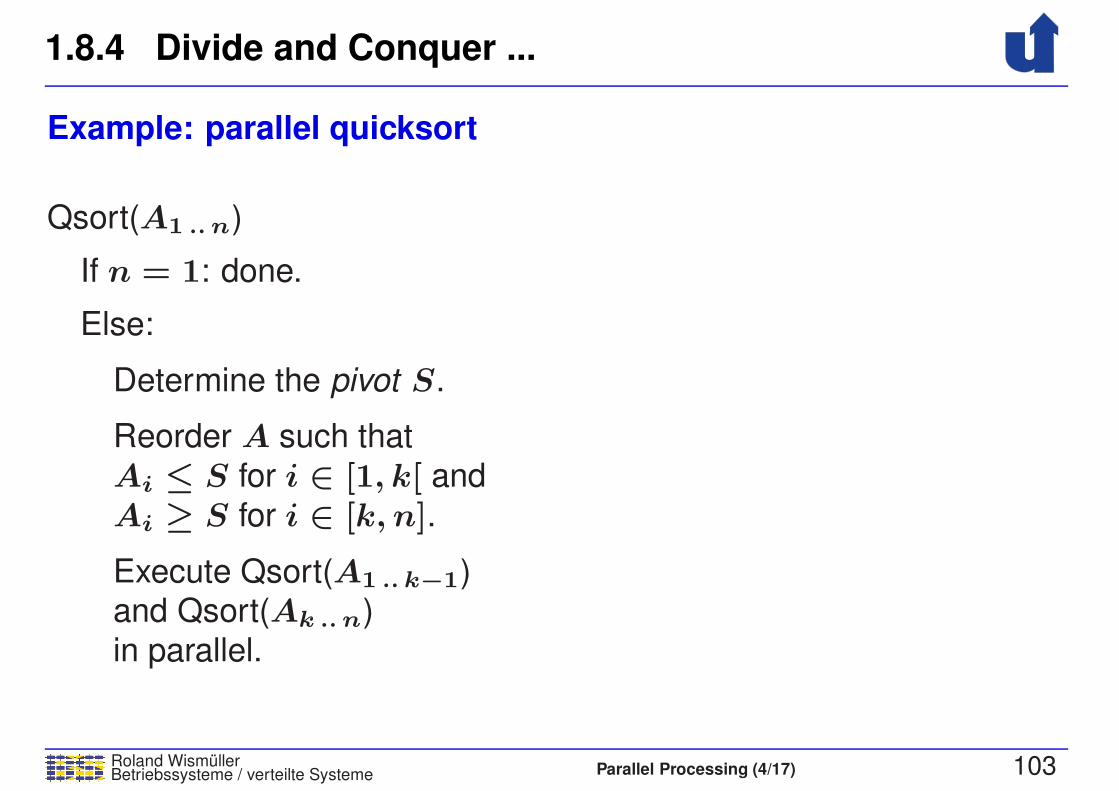
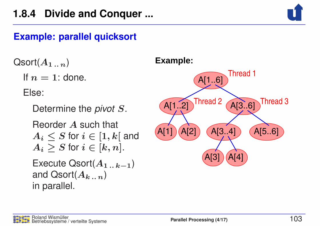
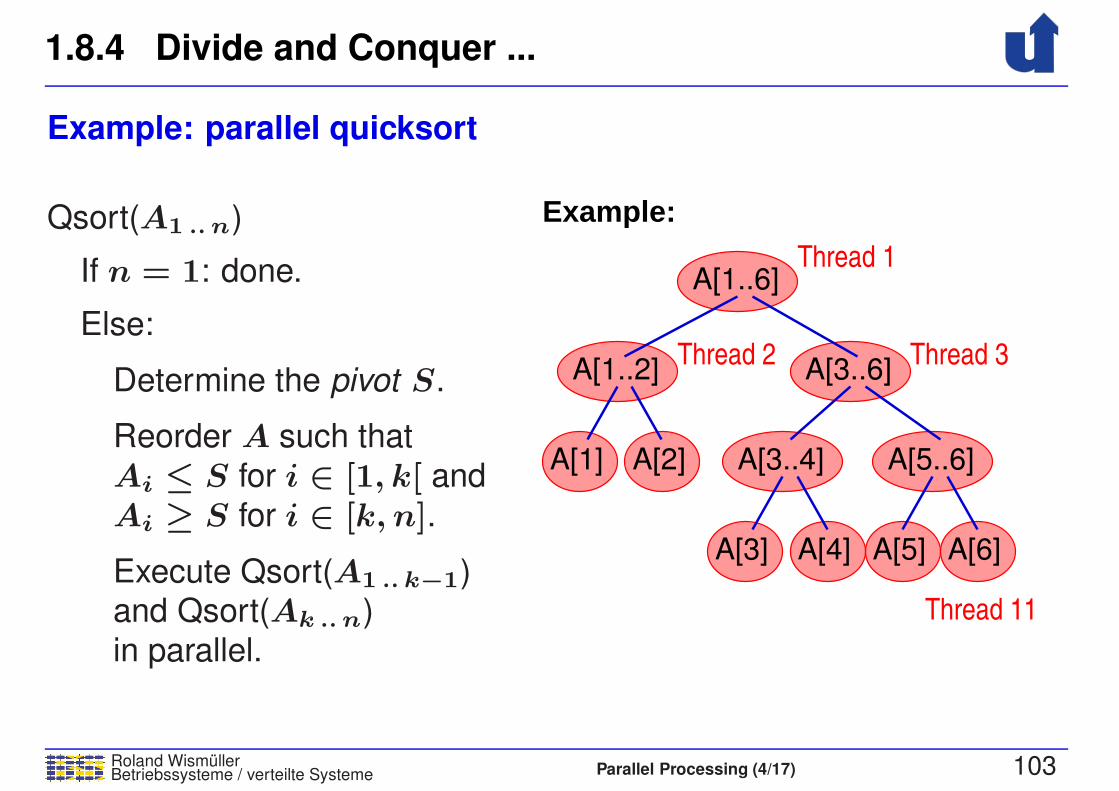
Example: parallel quicksort
Qsort(A1 .. n)
If n = 1: done.
Else:
Determine the pivot S.
Reorder A such that
Ai ≤ S for i ∈ [1, k[ and
Ai ≥ S for i ∈ [k, n].
Execute Qsort(A1 .. k−1)and Qsort(Ak .. n)
in parallel.
1.8.4 Divide and Conquer ...
Roland WismullerBetriebssysteme / verteilte Systeme Parallel Processing (4/17) 103
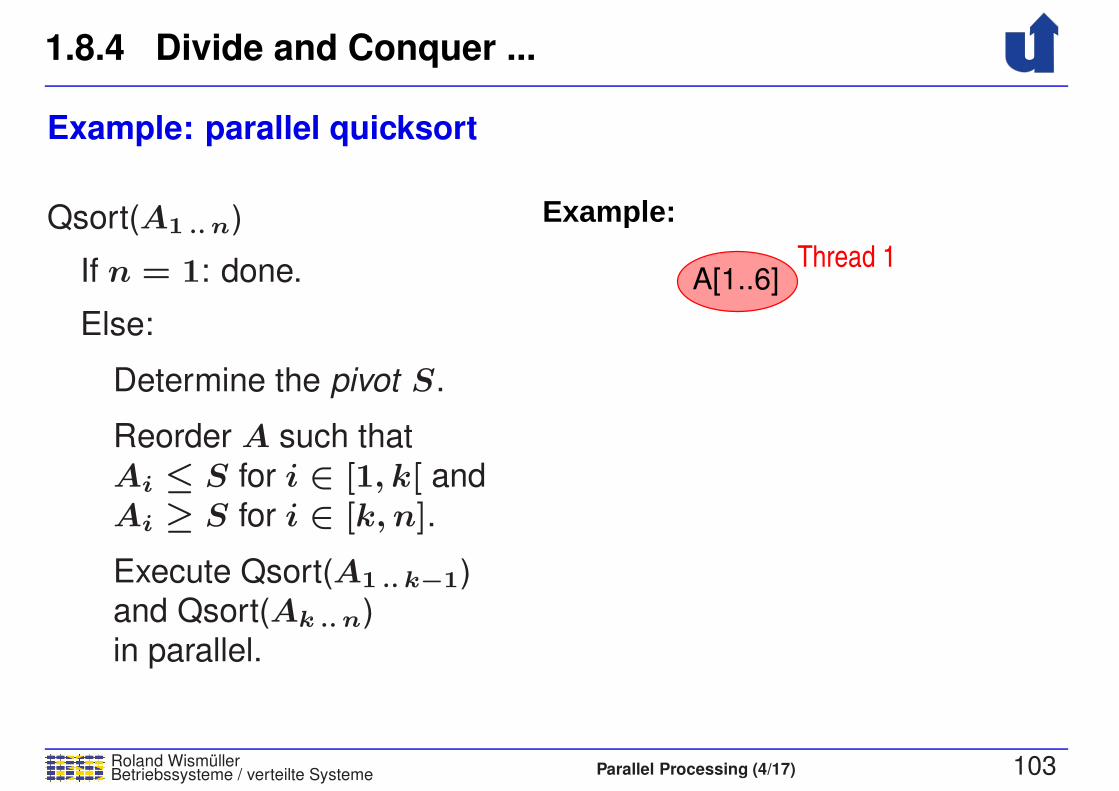
Example: parallel quicksort
Qsort(A1 .. n)
If n = 1: done.
Else:
Determine the pivot S.
Reorder A such that
Ai ≤ S for i ∈ [1, k[ and
Ai ≥ S for i ∈ [k, n].
Execute Qsort(A1 .. k−1)and Qsort(Ak .. n)
in parallel.
Thread 1A[1..6]
Example:
1.8.4 Divide and Conquer ...
Roland WismullerBetriebssysteme / verteilte Systeme Parallel Processing (4/17) 103
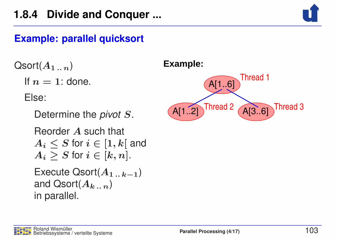
Example: parallel quicksort
Qsort(A1 .. n)
If n = 1: done.
Else:
Determine the pivot S.
Reorder A such that
Ai ≤ S for i ∈ [1, k[ and
Ai ≥ S for i ∈ [k, n].
Execute Qsort(A1 .. k−1)and Qsort(Ak .. n)
in parallel.
Thread 2 Thread 3
Thread 1
A[3..6]A[1..2]
A[1..6]
Example:

1.8.4 Divide and Conquer ...
Roland WismullerBetriebssysteme / verteilte Systeme Parallel Processing (4/17) 103
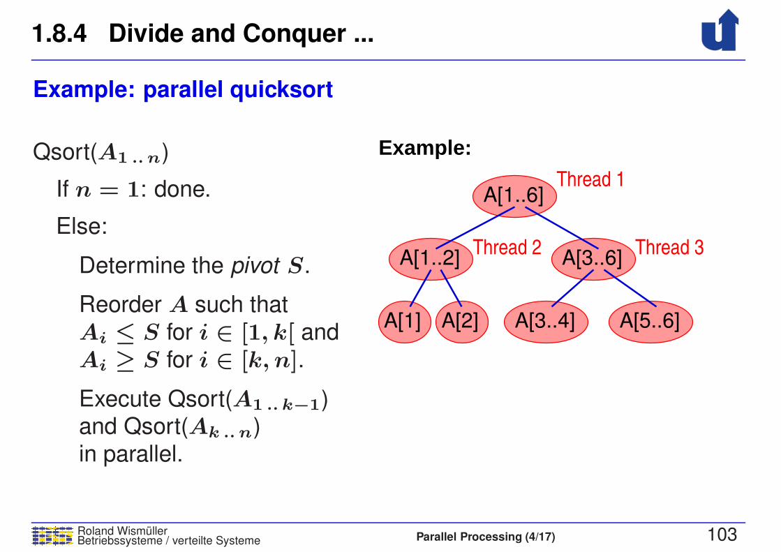
Example: parallel quicksort
Qsort(A1 .. n)
If n = 1: done.
Else:
Determine the pivot S.
Reorder A such that
Ai ≤ S for i ∈ [1, k[ and
Ai ≥ S for i ∈ [k, n].
Execute Qsort(A1 .. k−1)and Qsort(Ak .. n)
in parallel.
Thread 2 Thread 3
Thread 1
A[2]A[1]
A[3..6]A[1..2]
A[1..6]
Example:
1.8.4 Divide and Conquer ...
Roland WismullerBetriebssysteme / verteilte Systeme Parallel Processing (4/17) 103
Example: parallel quicksort
Qsort(A1 .. n)
If n = 1: done.
Else:
Determine the pivot S.
Reorder A such that
Ai ≤ S for i ∈ [1, k[ and
Ai ≥ S for i ∈ [k, n].
Execute Qsort(A1 .. k−1)and Qsort(Ak .. n)
in parallel.
Thread 2 Thread 3
Thread 1
A[3..4] A[5..6]A[2]A[1]
A[3..6]A[1..2]
A[1..6]
Example:
1.8.4 Divide and Conquer ...
Roland WismullerBetriebssysteme / verteilte Systeme Parallel Processing (4/17) 103
Example: parallel quicksort
Qsort(A1 .. n)
If n = 1: done.
Else:
Determine the pivot S.
Reorder A such that
Ai ≤ S for i ∈ [1, k[ and
Ai ≥ S for i ∈ [k, n].
Execute Qsort(A1 .. k−1)and Qsort(Ak .. n)
in parallel.
Thread 2 Thread 3
Thread 1
A[3] A[4]
A[3..4] A[5..6]A[2]A[1]
A[3..6]A[1..2]
A[1..6]
Example:
1.8.4 Divide and Conquer ...
Roland WismullerBetriebssysteme / verteilte Systeme Parallel Processing (4/17) 103
Example: parallel quicksort
Qsort(A1 .. n)
If n = 1: done.
Else:
Determine the pivot S.
Reorder A such that
Ai ≤ S for i ∈ [1, k[ and
Ai ≥ S for i ∈ [k, n].
Execute Qsort(A1 .. k−1)and Qsort(Ak .. n)
in parallel.
Thread 11
Thread 2 Thread 3
Thread 1
A[5] A[6]A[3] A[4]
A[3..4] A[5..6]A[2]A[1]
A[3..6]A[1..2]
A[1..6]
Example:
1.8.4 Divide and Conquer ...
Roland WismullerBetriebssysteme / verteilte Systeme Parallel Processing (4/17) 104
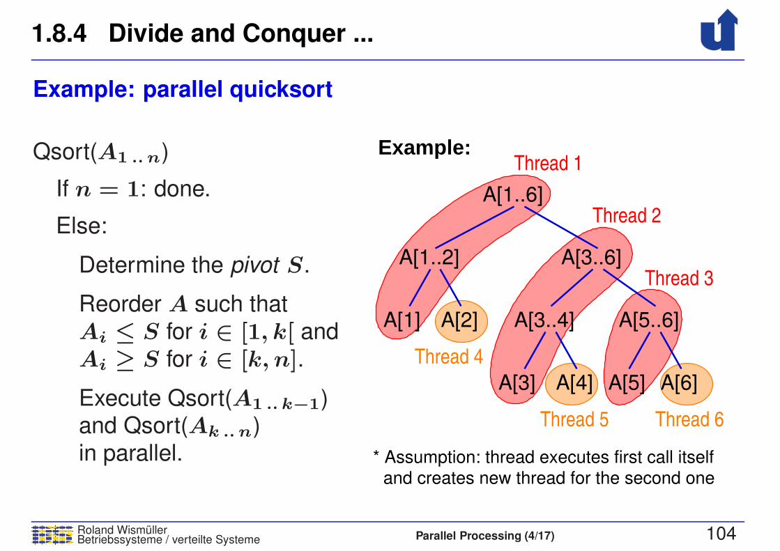
Example: parallel quicksort
Qsort(A1 .. n)
If n = 1: done.
Else:
Determine the pivot S.
Reorder A such that
Ai ≤ S for i ∈ [1, k[ and
Ai ≥ S for i ∈ [k, n].
Execute Qsort(A1 .. k−1)and Qsort(Ak .. n)
in parallel. * Assumption: thread executes first call itselfand creates new thread for the second one
Thread 1
Thread 2
Thread 3
Thread 4
Thread 5 Thread 6
A[5] A[6]A[3] A[4]
A[3..4] A[5..6]A[2]A[1]
A[3..6]A[1..2]
A[1..6]
Example:
1.8.4 Divide and Conquer ...
Roland WismullerBetriebssysteme / verteilte Systeme Parallel Processing (4/17) 105
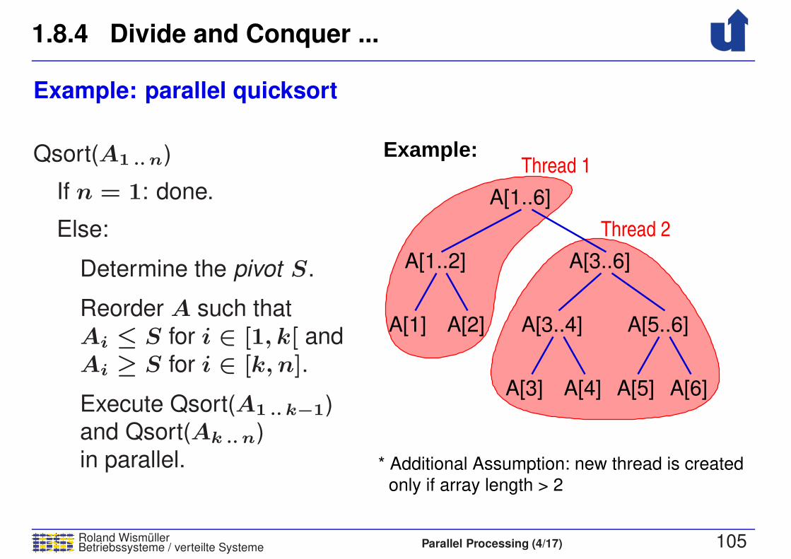
Example: parallel quicksort
Qsort(A1 .. n)
If n = 1: done.
Else:
Determine the pivot S.
Reorder A such that
Ai ≤ S for i ∈ [1, k[ and
Ai ≥ S for i ∈ [k, n].
Execute Qsort(A1 .. k−1)and Qsort(Ak .. n)
in parallel. * Additional Assumption: new thread is created
Thread 2
Thread 1
only if array length > 2
A[5] A[6]A[3] A[4]
A[3..4] A[5..6]A[2]A[1]
A[3..6]A[1..2]
A[1..6]
Example:

1.8 Organisation Forms for Parallel Programs ...
Roland WismullerBetriebssysteme / verteilte Systeme Parallel Processing (4/17) 106
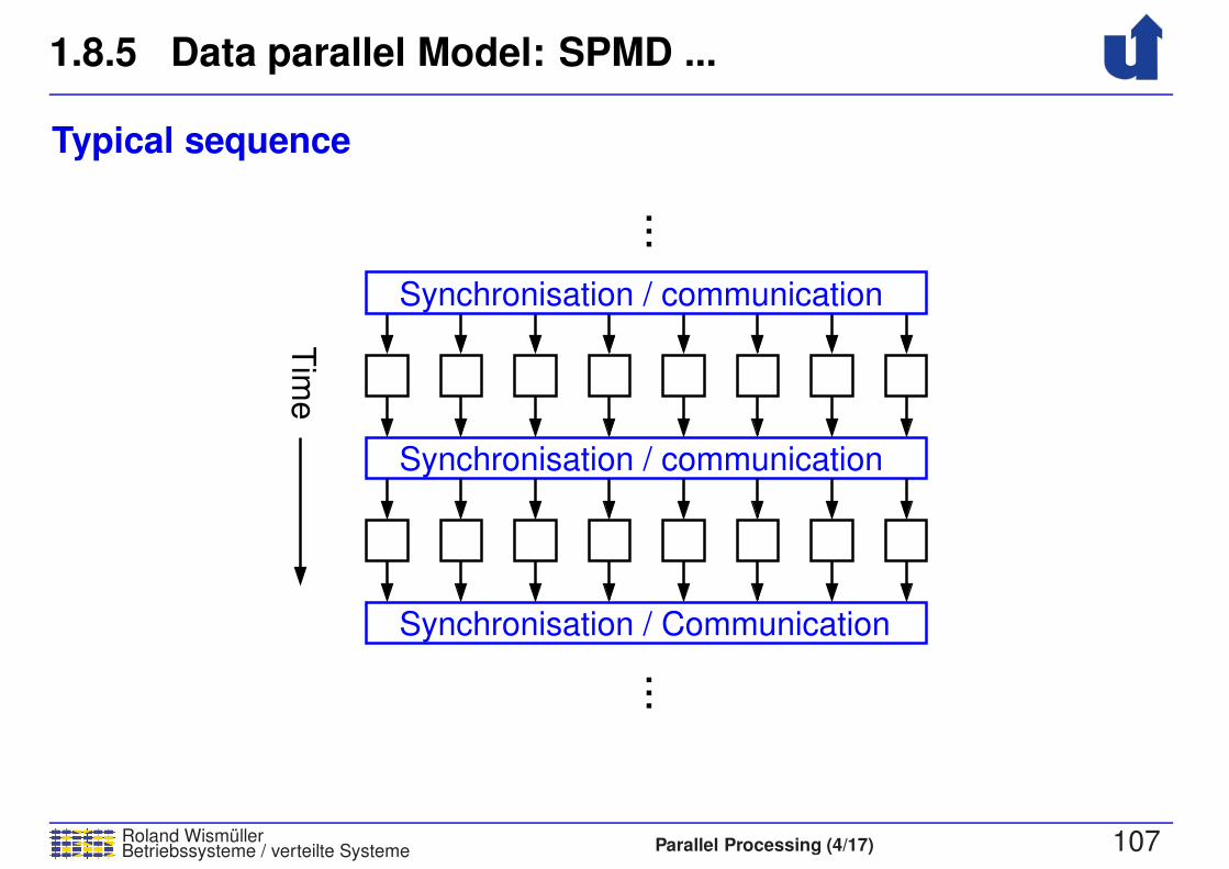
1.8.5 Data parallel Model: SPMD
➥ Fixed, constant number of processes (or threads, respectively)
➥ One-to-one correspondence between tasks and processes
➥ All processes execute the same program code
➥ however: conditional statements are possible ...
➥ For program parts which cannot be parallelised:
➥ replicated execution in each process
➥ execution in only one process; the other ones wait
➥ Usually loosely synchronous execution:
➥ alternating phases with independent computations and
communication / synchronisation
1.8.5 Data parallel Model: SPMD ...
Roland WismullerBetriebssysteme / verteilte Systeme Parallel Processing (4/17) 107
Typical sequence
......
Synchronisation / communication
Synchronisation / communication
Synchronisation / Communication
Tim
e

1.8 Organisation Forms for Parallel Programs ...
Roland WismullerBetriebssysteme / verteilte Systeme Parallel Processing (4/17) 108
1.8.6 Fork/Join Model
➥ Program consists of sequential
and parallel phases
➥ Thread (or processes, resp.) for
parallel phases are created at
run-time (fork )
➥ one for each task
➥ At the end of each parallel
phase: synchronisation and
termination of the threads (join)
Fork
Join
Tim
e
1.8 Organisation Forms for Parallel Programs ...
Roland WismullerBetriebssysteme / verteilte Systeme Parallel Processing (4/17) 109
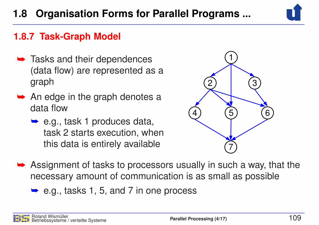
1.8.7 Task-Graph Model
➥ Tasks and their dependences
(data flow) are represented as a
graph
➥ An edge in the graph denotes a
data flow
➥ e.g., task 1 produces data,
task 2 starts execution, when
this data is entirely available
3
4 5 6
7
1
2
➥ Assignment of tasks to processors usually in such a way, that the
necessary amount of communication is as small as possible
➥ e.g., tasks 1, 5, and 7 in one process
1.8 Organisation Forms for Parallel Programs ...
Roland WismullerBetriebssysteme / verteilte Systeme Parallel Processing (4/17) 110
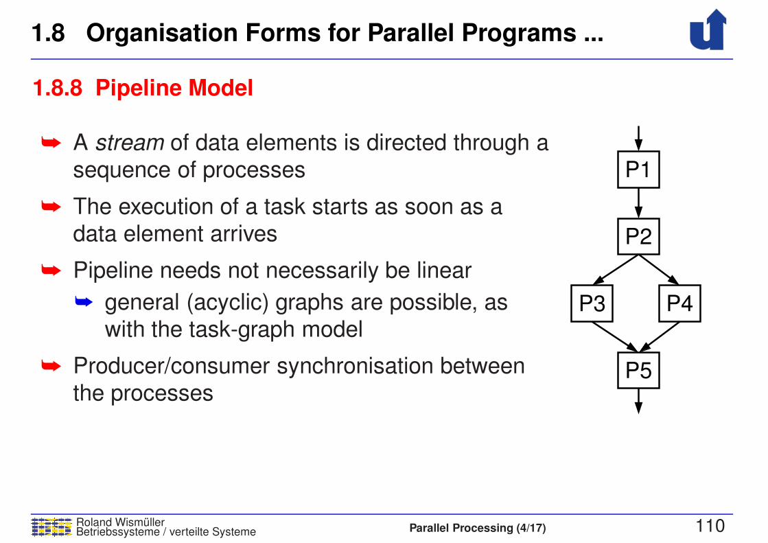
1.8.8 Pipeline Model
➥ A stream of data elements is directed through a
sequence of processes
➥ The execution of a task starts as soon as a
data element arrives
➥ Pipeline needs not necessarily be linear
➥ general (acyclic) graphs are possible, as
with the task-graph model
➥ Producer/consumer synchronisation between
the processes
P1
P2
P3 P4
P5
1.9 Performance Considerations
Roland WismullerBetriebssysteme / verteilte Systeme Parallel Processing (4/17) 111
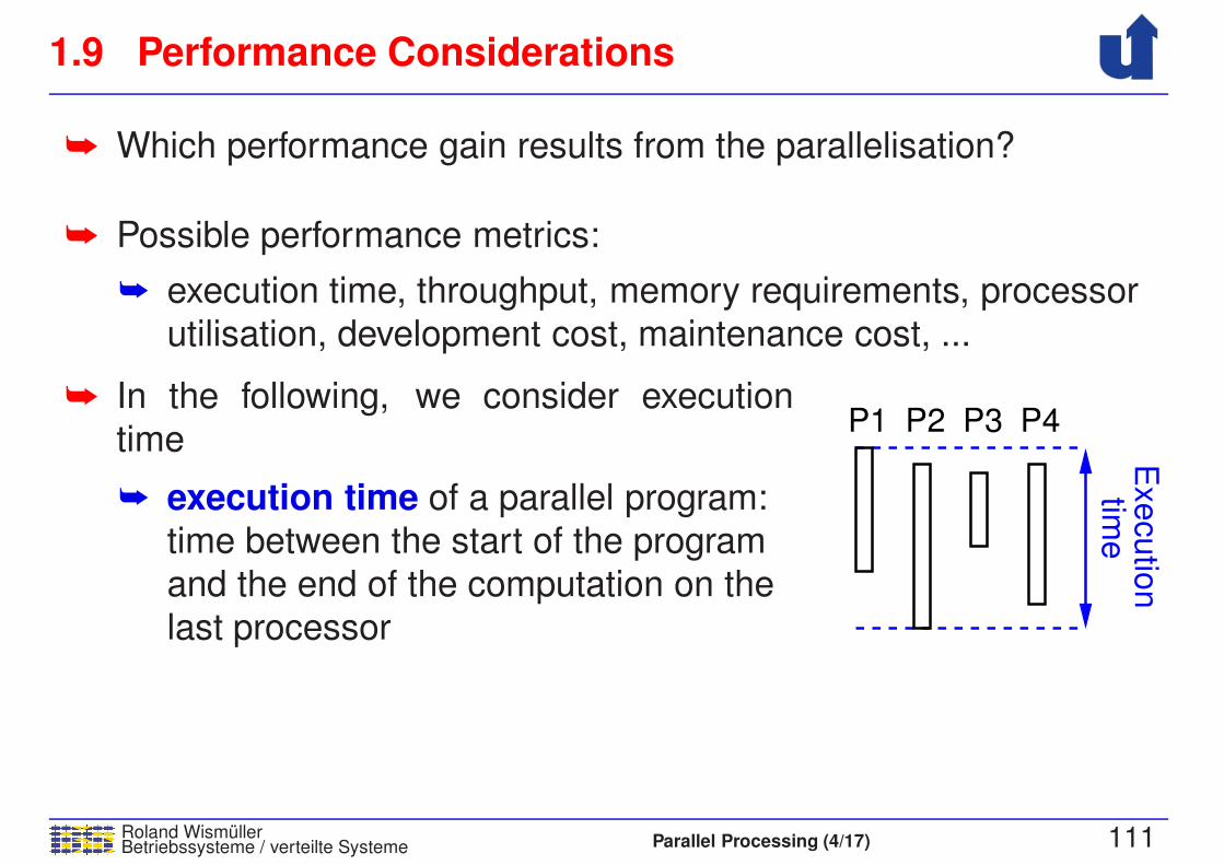
➥ Which performance gain results from the parallelisation?
➥ Possible performance metrics:
➥ execution time, throughput, memory requirements, processor
utilisation, development cost, maintenance cost, ...
➥ In the following, we consider execution
time
➥ execution time of a parallel program:
time between the start of the program
and the end of the computation on the
last processor
P1 P2 P3 P4
time
Executio
n
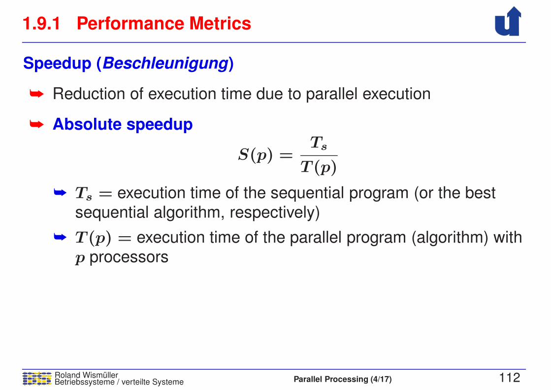
1.9.1 Performance Metrics
Roland WismullerBetriebssysteme / verteilte Systeme Parallel Processing (4/17) 112
Speedup (Beschleunigung)
➥ Reduction of execution time due to parallel execution
➥ Absolute speedup
S(p) =Ts
T (p)
➥ Ts = execution time of the sequential program (or the best
sequential algorithm, respectively)
➥ T (p) = execution time of the parallel program (algorithm) with
p processors

1.9.1 Performance Metrics ...
Roland WismullerBetriebssysteme / verteilte Systeme Parallel Processing (4/17) 113
Speedup (Beschleunigung) ...
➥ Relative speedup (for “sugarcoated” results ...)
S(p) =T (1)
T (p)
➥ T (1) = execution time of the parallel program (algorithm) with
one processor
➥ Optimum: S(p) = p
➥ Often: with fixed problem size, S(p) declines again, when pincreases
➥ more communication, less computing work per processor
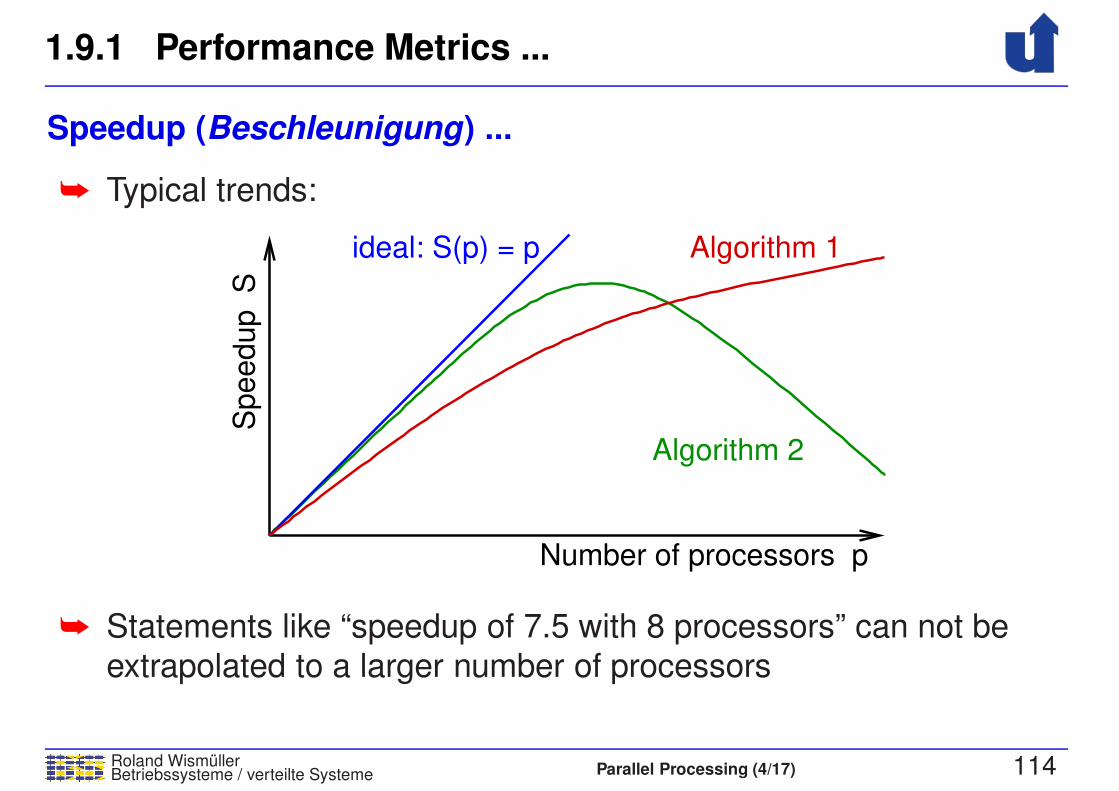
1.9.1 Performance Metrics ...
Roland WismullerBetriebssysteme / verteilte Systeme Parallel Processing (4/17) 114
Speedup (Beschleunigung) ...
➥ Typical trends:
Algorithm 2
Algorithm 1
Number of processors p
Speedup S
ideal: S(p) = p
➥ Statements like “speedup of 7.5 with 8 processors” can not be
extrapolated to a larger number of processors
1.9.1 Performance Metrics ...
Roland WismullerBetriebssysteme / verteilte Systeme Parallel Processing (4/17) 115
Superlinear speedup
➥ Sometimes we observe S(p) > p, although this should actually
be impossible
➥ Causes:
➥ implicit change in the algorithm
➥ e.g., with parallel tree search: several paths in the search
tree are traversed simultaneously
➥ limited breadth-first search instead of depth-first search
➥ cache effects
➥ with p processors, the amount of cache is p times higher
that with one processor
➥ thus, we also have higher cache hit rates
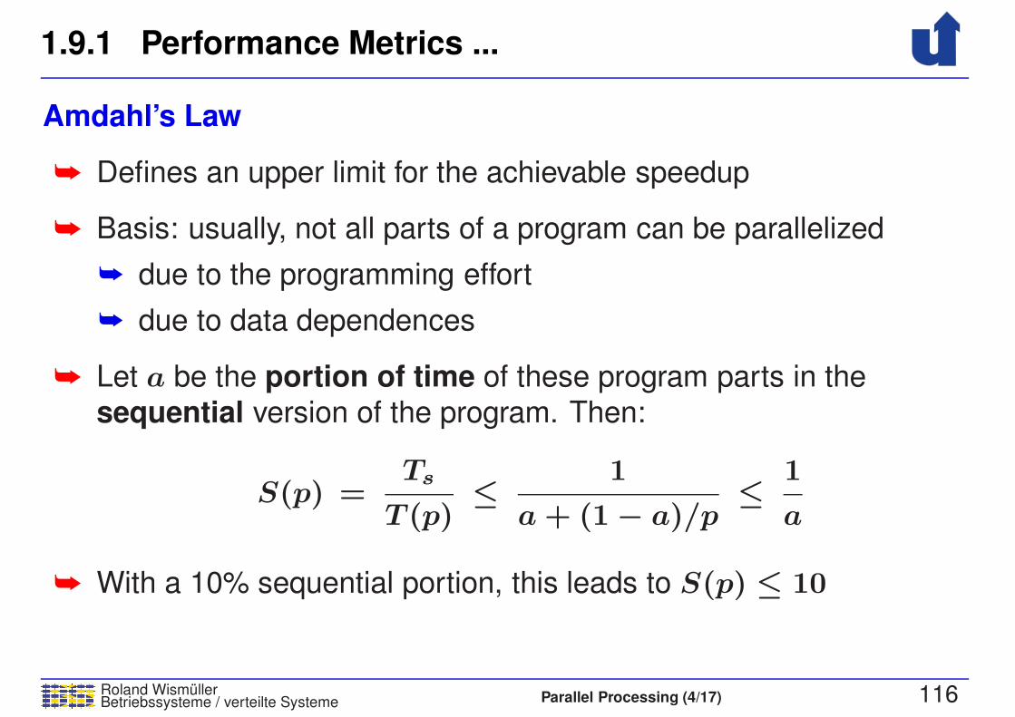
1.9.1 Performance Metrics ...
Roland WismullerBetriebssysteme / verteilte Systeme Parallel Processing (4/17) 116
Amdahl’s Law
➥ Defines an upper limit for the achievable speedup
➥ Basis: usually, not all parts of a program can be parallelized
➥ due to the programming effort
➥ due to data dependences
➥ Let a be the portion of time of these program parts in the
sequential version of the program. Then:
S(p) =Ts
T (p)≤ 1
a + (1− a)/p≤ 1
a
➥ With a 10% sequential portion, this leads to S(p) ≤ 10
1.9.1 Performance Metrics ...
Roland WismullerBetriebssysteme / verteilte Systeme Parallel Processing (4/17) 117
Efficiency
E(p) =S(p)
p
➥ Metrics for the utilisation of a parallel computer
➥ E(p) ≤ 1, the optimum would be E(p) = 1
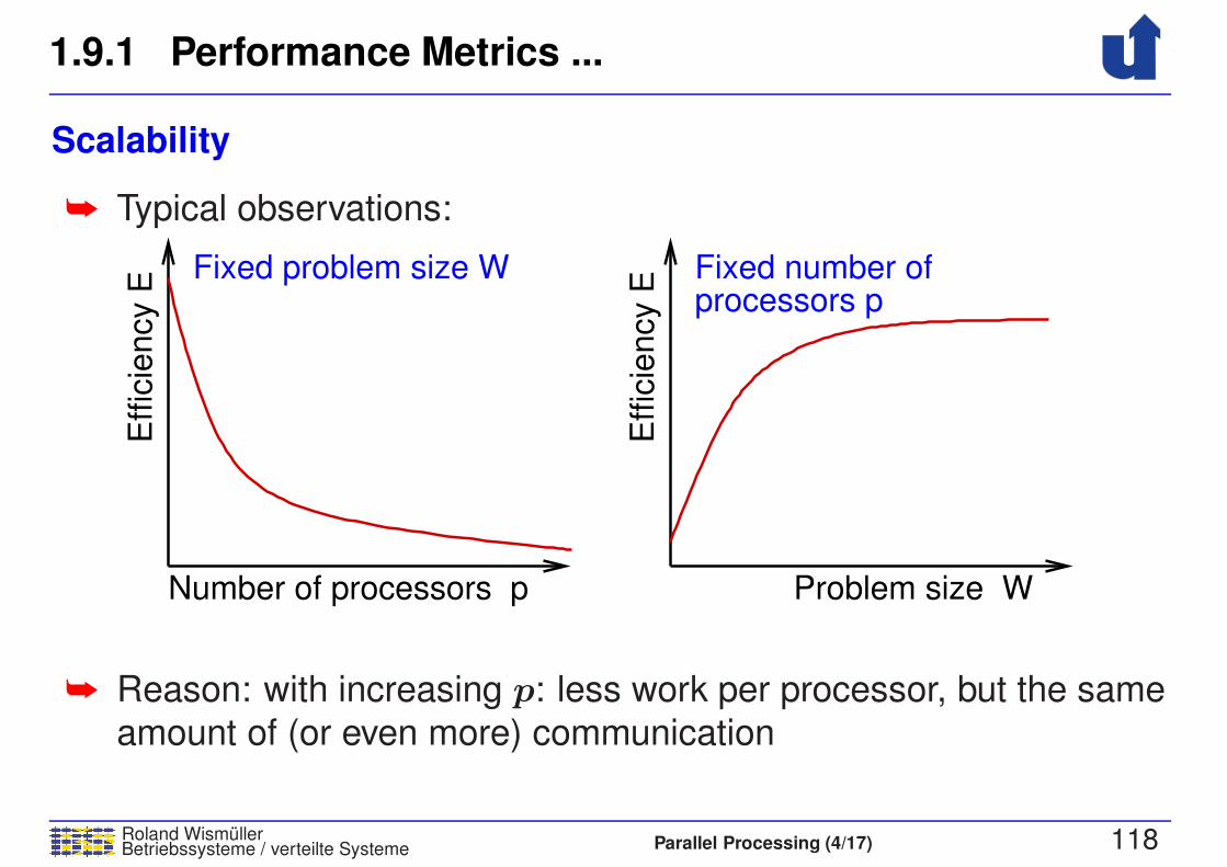
1.9.1 Performance Metrics ...
Roland WismullerBetriebssysteme / verteilte Systeme Parallel Processing (4/17) 118
Scalability
➥ Typical observations:
Problem size WNumber of processors p
Fixed problem size Wprocessors pFixed number of
Effic
iency E
Effic
iency E
➥ Reason: with increasing p: less work per processor, but the same
amount of (or even more) communication

1.9.1 Performance Metrics ...
Roland WismullerBetriebssysteme / verteilte Systeme Parallel Processing (4/17) 119
Scalability ...
➥ How must the problem size W increase with increasing numberof processors p, such that the efficiency stays the same?
➥ Answer is given by the isoefficiency function
➥ Parallel execution time
T (p) =W + To(W,p)
p
➥ To(W,p) = overhead of parallel execution
➥ T and W are measured as the number of elementaryoperations
➥ Thus:
W =E
1− E· To(W,p)
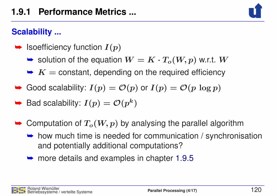
1.9.1 Performance Metrics ...
Roland WismullerBetriebssysteme / verteilte Systeme Parallel Processing (4/17) 120
Scalability ...
➥ Isoefficiency function I(p)
➥ solution of the equation W = K · To(W,p) w.r.t. W
➥ K = constant, depending on the required efficiency
➥ Good scalability: I(p) = O(p) or I(p) = O(p log p)
➥ Bad scalability: I(p) = O(pk)
➥ Computation of To(W,p) by analysing the parallel algorithm
➥ how much time is needed for communication / synchronisationand potentially additional computations?
➥ more details and examples in chapter 1.9.5

1.9.2 Reasons for Performance Loss
Roland WismullerBetriebssysteme / verteilte Systeme Parallel Processing (4/17) 121
➥ Access losses due to data exchange between tasks
➥ e.g., message passing, remote memory access
➥ Conflict losses due to shared use of ressources by multiple
tasks
➥ e.g., conflicts when accessing the network, mutual exclusion
when accessing data
➥ Utilisation losses due to insufficent degree of parallelism
➥ e.g., waiting for data, load imbalance
➥ Breaking losses when computations should end
➥ e.g., with search problems: all other processes must benotified that a solution has been found

1.9.2 Reasons for Performance Loss ...
Roland WismullerBetriebssysteme / verteilte Systeme Parallel Processing (4/17) 122
➥ Complexity losses due to additional work neccessary for the
parallel execution
➥ e.g., partitioning of unstructured grids
➥ Dumping losses due to computations, which are executed
redundantly but not used later on
➥ e.g., lapsed search in branch-and-bound algorithms
➥ Algorithmic losses due to modifications of the algorithms during
the parallelisation
➥ e.g., worse convergence of an iterative method
Roland WismullerBetriebssysteme / verteilte Systeme Parallel Processing (5/17) vi
Roland Wismuller
Universitat Siegen
Tel.: 0271/740-4050, Buro: H-B 8404
Stand: January 23, 2018
Parallel Processing
WS 2017/18
23.10.2017
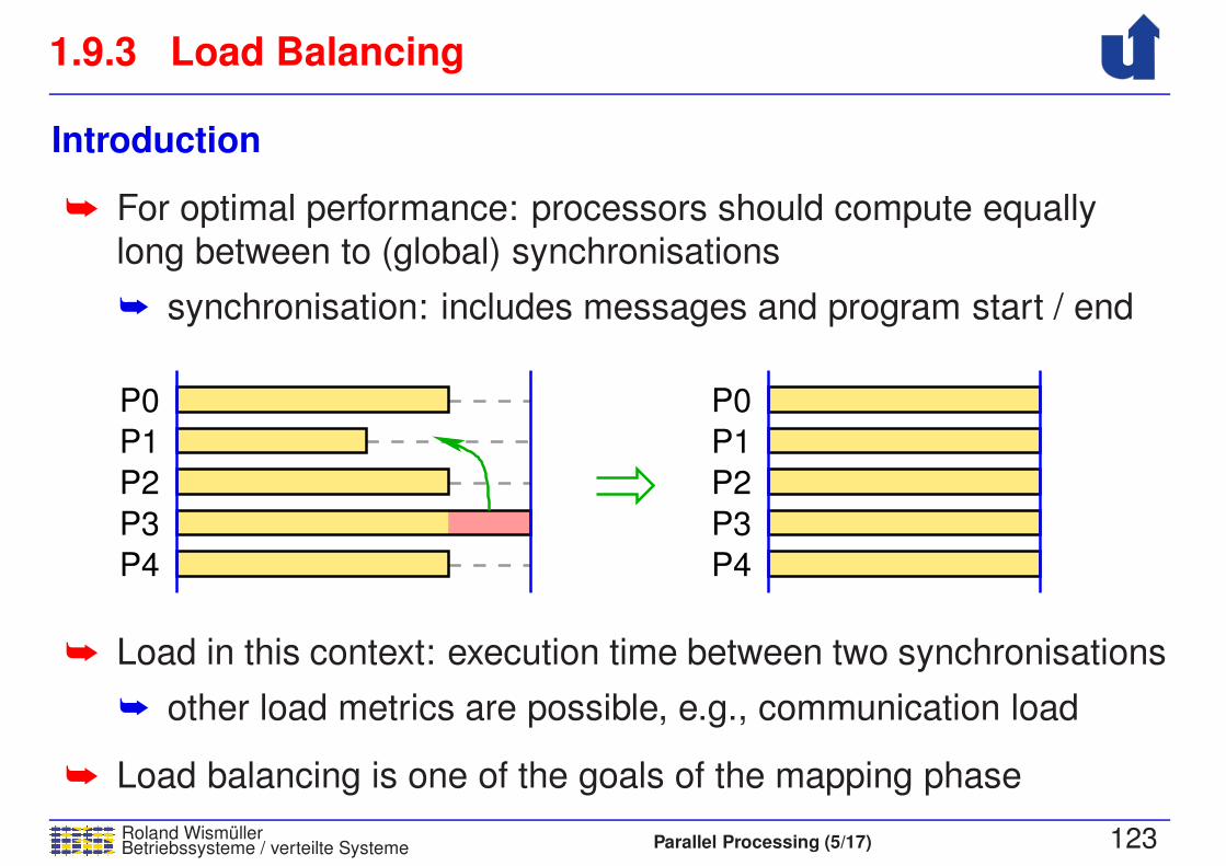
1.9.3 Load Balancing
Roland WismullerBetriebssysteme / verteilte Systeme Parallel Processing (5/17) 123
Introduction
➥ For optimal performance: processors should compute equally
long between to (global) synchronisations
➥ synchronisation: includes messages and program start / end
P0
P1
P2
P3
P4
P0
P1
P2
P3
P4
➥ Load in this context: execution time between two synchronisations
➥ other load metrics are possible, e.g., communication load
➥ Load balancing is one of the goals of the mapping phase
1.9.3 Load Balancing ...
Roland WismullerBetriebssysteme / verteilte Systeme Parallel Processing (5/17) 124
Reasons for load imbalance
➥ Unequal computational load of the tasks
➥ e.g., atmospheric model: areas over land / water
➥ Heterogeneous execution plattform
➥ e.g., processors with different speed
➥ Computational load of the tasks changes dynamically
➥ e.g., in atmospheric model, depending on the simulated
time of day (solar radiation)
➥ Background load on the processors
➥ e.g., in a PC cluster
dynam
icsta
tic
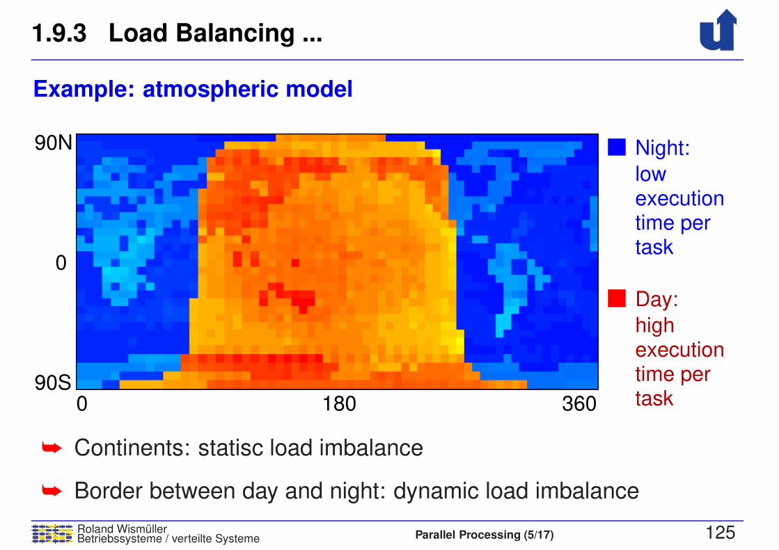
1.9.3 Load Balancing ...
Roland WismullerBetriebssysteme / verteilte Systeme Parallel Processing (5/17) 125
Example: atmospheric model
executiontime pertask
high
Day:
lowexecutiontime pertask
Night:
90S0
0
90N
180 360
➥ Continents: statisc load imbalance
➥ Border between day and night: dynamic load imbalance

1.9.3 Load Balancing ...
Roland WismullerBetriebssysteme / verteilte Systeme Parallel Processing (5/17) 125
Example: atmospheric model
executiontime pertask
high
Day:
lowexecutiontime pertask
Night:
90S0
0
90N
180 360
0 1 2 3
➥ Continents: statisc load imbalance
➥ Border between day and night: dynamic load imbalance

1.9.3 Load Balancing ...
Roland WismullerBetriebssysteme / verteilte Systeme Parallel Processing (5/17) 126
Static load balancing
➥ Goal: distribute the tasks to the processors at / before program
start, such that the computational load of the processors is equal
➥ Two fundamentally different approaches:
➥ take into account the tasks’ different computational load when
mapping them to processors
➥ extension of graph partitioning algorithms
➥ requires a good estimation of a task’s load
➥ no solution, when load changes dynamically
➥ fine grained cyclic or random mapping
➥ results (most likely) in a good load balancing, even when
the load changes dynamically
➥ price: usually higher communication cost

1.9.3 Load Balancing ...
Roland WismullerBetriebssysteme / verteilte Systeme Parallel Processing (5/17) 127
Example: atmospheric model, cyclic mapping
executiontime pertask
high
Day:
lowexecutiontime pertask
Night:
90S0
0
90N
180 360
0 1 2 3 0 1 2 3 0 1 2 3 0 1 2 3 0 1 2 3
➥ Each processor has tasks with high and low computational load
1.9.3 Load Balancing ...
Roland WismullerBetriebssysteme / verteilte Systeme Parallel Processing (5/17) 128
Dynamic load balancing
➥ Independent (often dyn. created) tasks (e.g., search problem)
➥ goal: processors do not idle, i.e., always have a task to
process
➥ even at the end of the program, i.e., all processes finish at
the same time
➥ tasks are dynamically allocated to progessors and stay there
until their processing is finished
➥ optimal: allocate task with highest processing time first
➥ Communicating tasks (SPMD, e.g., stencil algorithm)
➥ goal: equal compunting time between synchronisations
➥ if necessary, tasks are migrated between processors during
their execution

1.9.4 Performance Analysis of Parallel Software
Roland WismullerBetriebssysteme / verteilte Systeme Parallel Processing (5/17) 129
How to determine performance metrics
➥ Analytical model of the algorithm
➥ approach: determine computation and communication time
➥ T (p) = tcomp + tcomm
➥ computation/communication ratio tcomp/tcomm allows a
rough estimation of performance
➥ requires a computation model (model of the computer
hardware)
➥ Measurement with the real programm
➥ explicit timing measurement in the code
➥ performance analysis tools
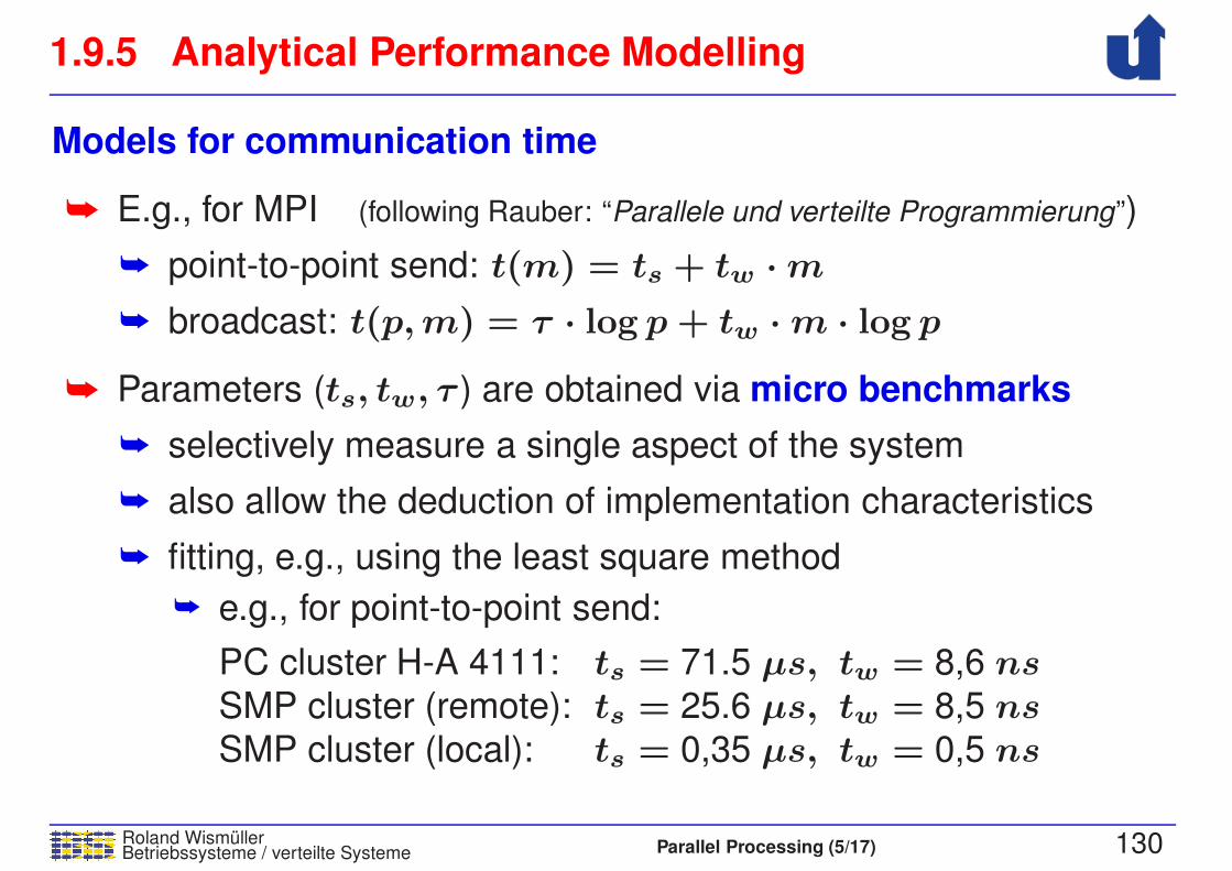
1.9.5 Analytical Performance Modelling
Roland WismullerBetriebssysteme / verteilte Systeme Parallel Processing (5/17) 130
Models for communication time
➥ E.g., for MPI (following Rauber: “Parallele und verteilte Programmierung”)
➥ point-to-point send: t(m) = ts + tw ·m➥ broadcast: t(p,m) = τ · log p + tw ·m · log p
➥ Parameters (ts, tw, τ ) are obtained via micro benchmarks
➥ selectively measure a single aspect of the system
➥ also allow the deduction of implementation characteristics
➥ fitting, e.g., using the least square method
➥ e.g., for point-to-point send:
PC cluster H-A 4111: ts = 71.5 µs, tw = 8,6 nsSMP cluster (remote): ts = 25.6 µs, tw = 8,5 nsSMP cluster (local): ts = 0,35 µs, tw = 0,5 ns
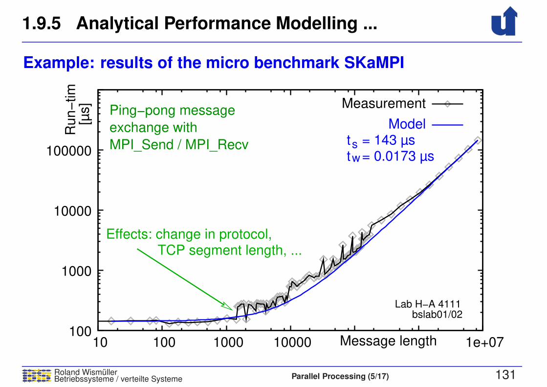
1.9.5 Analytical Performance Modelling ...
Roland WismullerBetriebssysteme / verteilte Systeme Parallel Processing (5/17) 131
Example: results of the micro benchmark SKaMPI
sw
t = 143 µs
Lab H−A 4111bslab01/02
t = 0.0173 µs
Effects: change in protocol,TCP segment length, ...
Message length
[µs]
Ru
n−
tim
e
Ping−pong message
exchange with
MPI_Send / MPI_Recv
Measurement
Model
100
1000
10000
100000
10 100 1000 10000 1e+07

1.9.5 Analytical Performance Modelling ...
Roland WismullerBetriebssysteme / verteilte Systeme Parallel Processing (5/17) 132
Communication protocols in MPI
ReceiverSender
Protocol
for short messages
MPI copiesmessage
MPI_Send
Rendezvous protocol
for long messages
ReceiverSender
messageis directly
MPI_Send
MPI_Recv
written todestinationbuffer
in dest. bufferMPI_Recv
MPI buffersmessage
Header (Sender,Tag, ...) + Data
Data
OK to send
Header

1.9.5 Analytical Performance Modelling ...
Roland WismullerBetriebssysteme / verteilte Systeme Parallel Processing (5/17) 133
Example: matrix multiplication
➥ Product C = A ·B of two square matrices
➥ Assumption: A, B, C are distributed blockwise on p processors
➥ processor Pij has Aij and Bij and computes Cij
➥ Pij needs Aik and Bkj for k = 1...√p
➥ Approach:
➥ all-to-all broadcast of the A blocks in each row of processors
➥ all-to-all broadcast of the B blocks in each column ofprocessors
➥ computation of Cij =
√p
∑
k=1
Aik ·Bkj
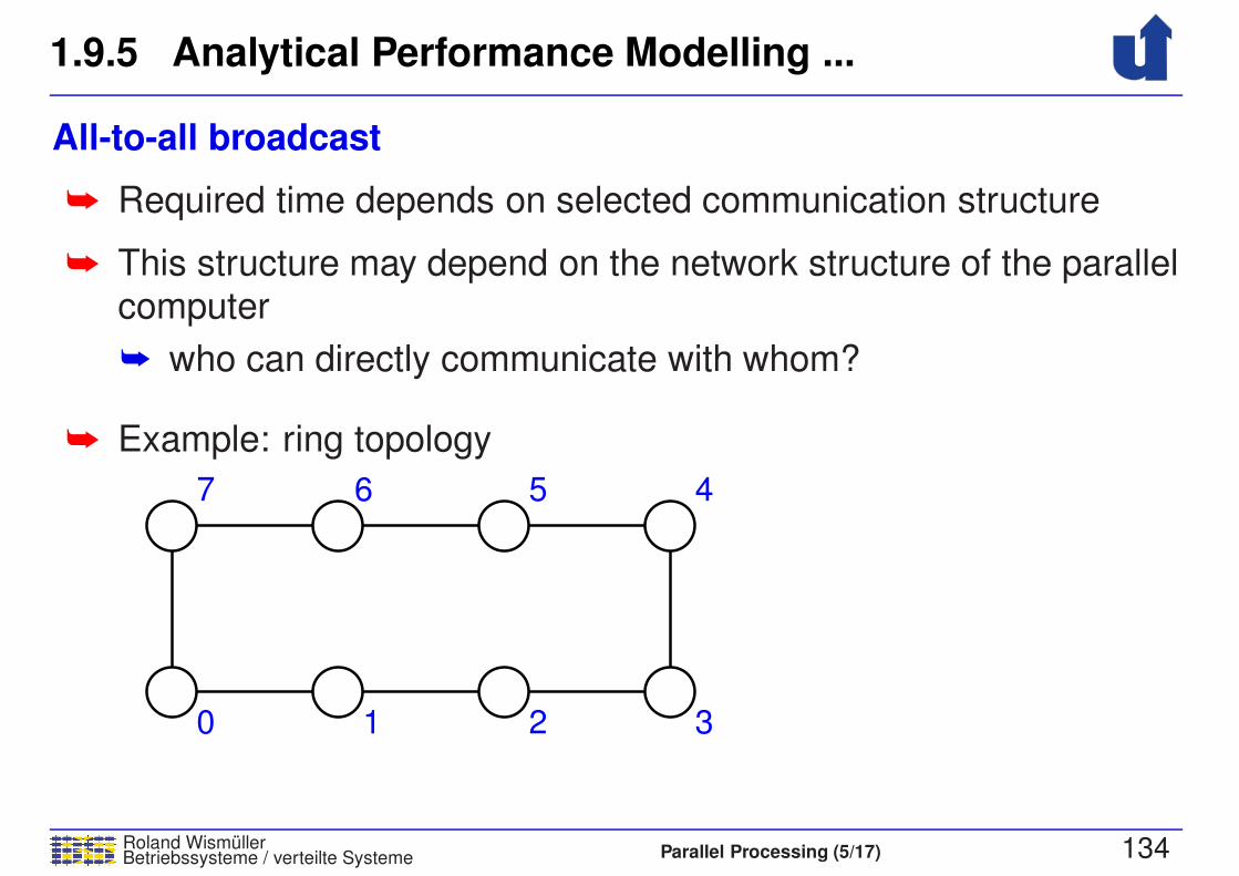
1.9.5 Analytical Performance Modelling ...
Roland WismullerBetriebssysteme / verteilte Systeme Parallel Processing (5/17) 134
All-to-all broadcast
➥ Required time depends on selected communication structure
➥ This structure may depend on the network structure of the parallelcomputer
➥ who can directly communicate with whom?
➥ Example: ring topology
320 1
67 5 4
➥ Cost: ts(p− 1) + twm(p− 1) (m: data length)
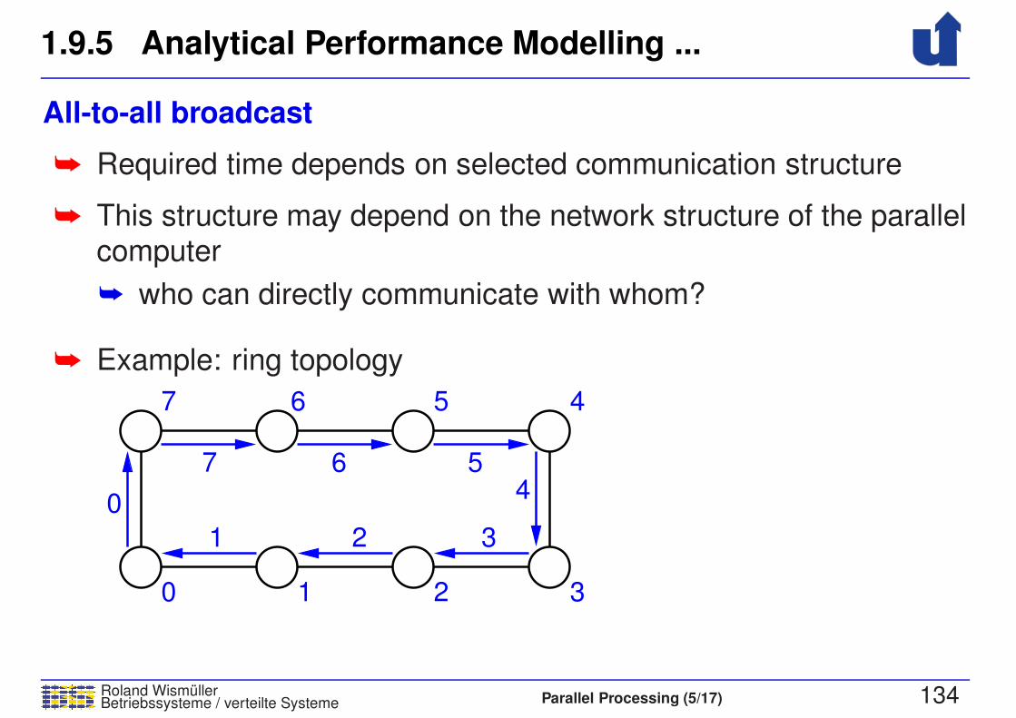
1.9.5 Analytical Performance Modelling ...
Roland WismullerBetriebssysteme / verteilte Systeme Parallel Processing (5/17) 134
All-to-all broadcast
➥ Required time depends on selected communication structure
➥ This structure may depend on the network structure of the parallelcomputer
➥ who can directly communicate with whom?
➥ Example: ring topology
320 1
67 5 4
321
0
7 564
➥ Cost: ts(p− 1) + twm(p− 1) (m: data length)
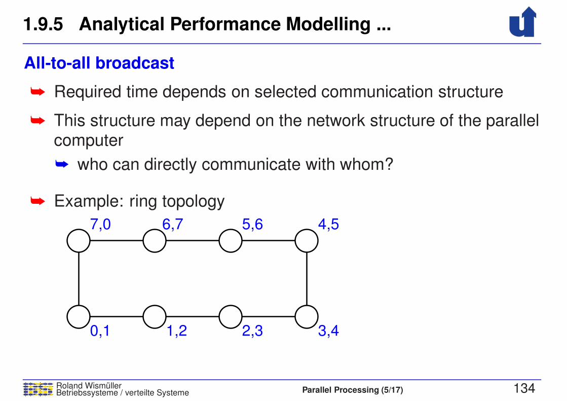
1.9.5 Analytical Performance Modelling ...
Roland WismullerBetriebssysteme / verteilte Systeme Parallel Processing (5/17) 134
All-to-all broadcast
➥ Required time depends on selected communication structure
➥ This structure may depend on the network structure of the parallelcomputer
➥ who can directly communicate with whom?
➥ Example: ring topology
0,1 1,2 2,3 3,4
4,55,66,77,0
➥ Cost: ts(p− 1) + twm(p− 1) (m: data length)
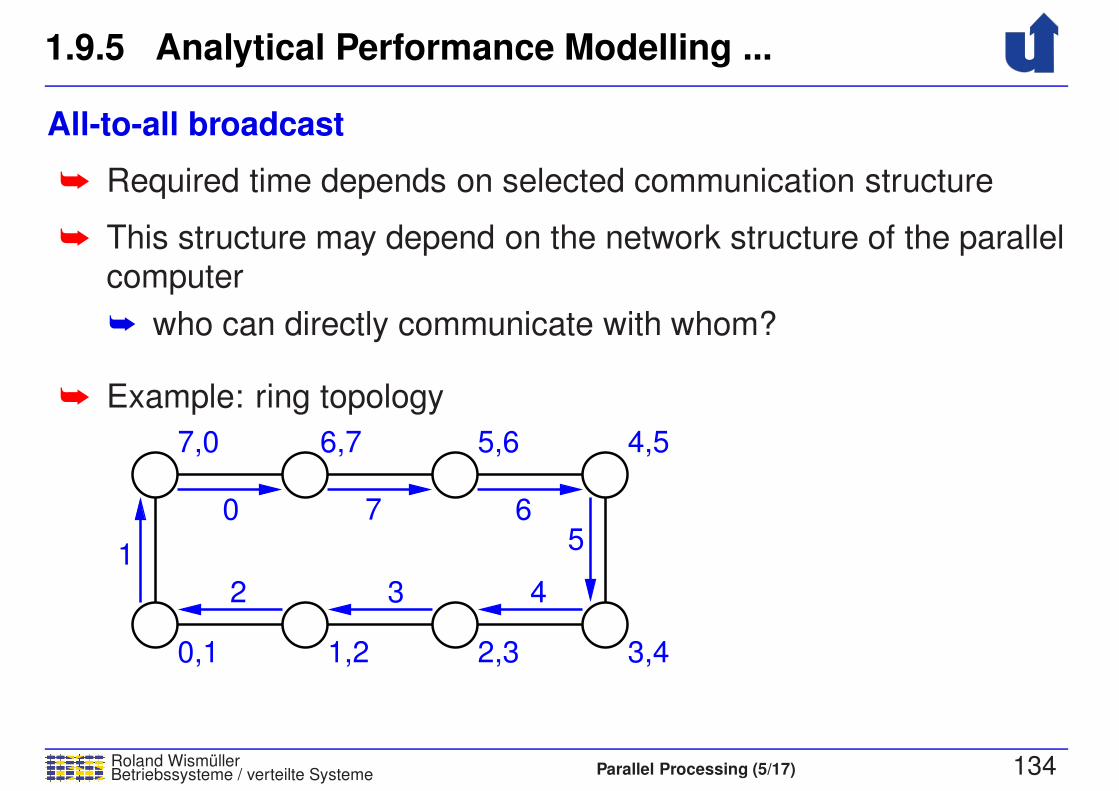
1.9.5 Analytical Performance Modelling ...
Roland WismullerBetriebssysteme / verteilte Systeme Parallel Processing (5/17) 134
All-to-all broadcast
➥ Required time depends on selected communication structure
➥ This structure may depend on the network structure of the parallelcomputer
➥ who can directly communicate with whom?
➥ Example: ring topology
0,1 1,2 2,3 3,4
4,55,66,77,0
0
1
2 3 4
567
➥ Cost: ts(p− 1) + twm(p− 1) (m: data length)

1.9.5 Analytical Performance Modelling ...
Roland WismullerBetriebssysteme / verteilte Systeme Parallel Processing (5/17) 134
All-to-all broadcast
➥ Required time depends on selected communication structure
➥ This structure may depend on the network structure of the parallelcomputer
➥ who can directly communicate with whom?
➥ Example: ring topology
0,1,2 1,2,3 2,3,4 3,4,5
4,5,65,6,76,7,07,0,1
➥ Cost: ts(p− 1) + twm(p− 1) (m: data length)
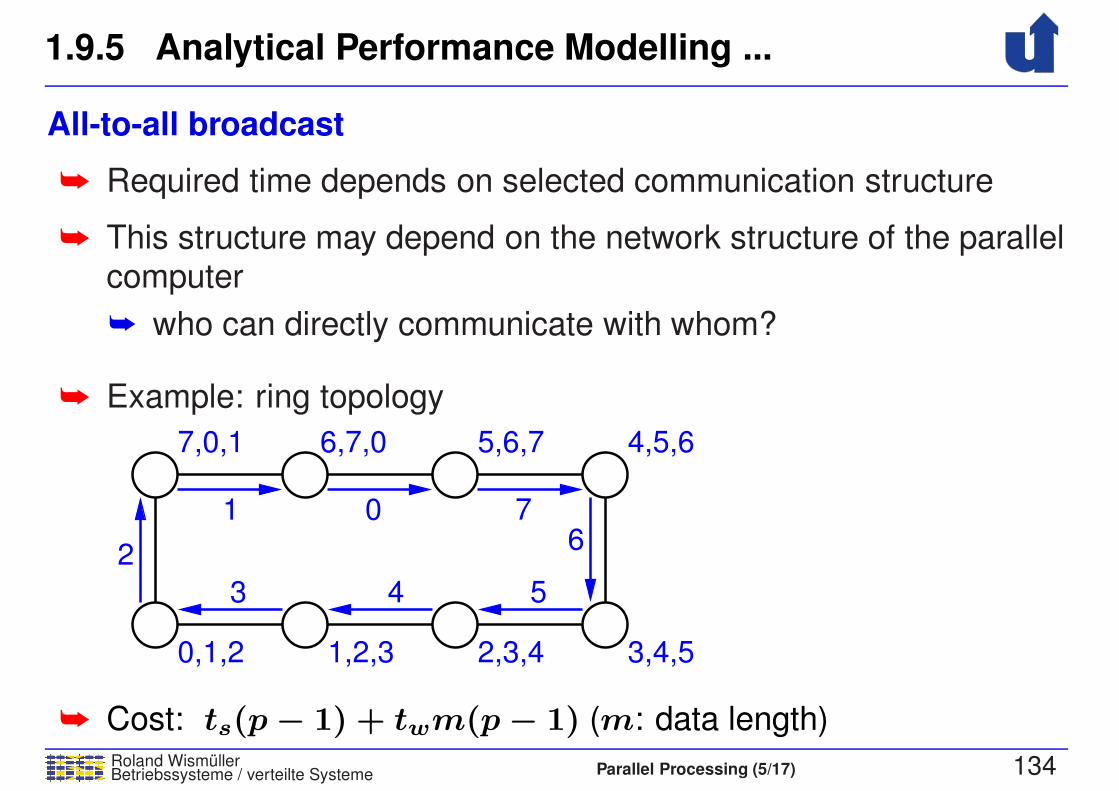
1.9.5 Analytical Performance Modelling ...
Roland WismullerBetriebssysteme / verteilte Systeme Parallel Processing (5/17) 134
All-to-all broadcast
➥ Required time depends on selected communication structure
➥ This structure may depend on the network structure of the parallelcomputer
➥ who can directly communicate with whom?
➥ Example: ring topology
0,1,2 1,2,3 2,3,4 3,4,5
4,5,65,6,76,7,07,0,1
01
2
3 4 5
67
➥ Cost: ts(p− 1) + twm(p− 1) (m: data length)
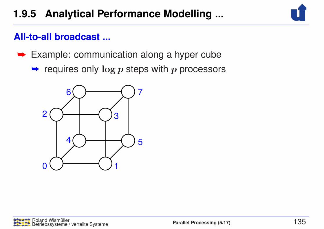
1.9.5 Analytical Performance Modelling ...
Roland WismullerBetriebssysteme / verteilte Systeme Parallel Processing (5/17) 135
All-to-all broadcast ...
➥ Example: communication along a hyper cube
➥ requires only log p steps with p processors
2
6 7
3
5
1
4
0
➥ Cost:
log p∑
i=1
(ts + 2i−1twm) = ts log p + twm(p− 1)

1.9.5 Analytical Performance Modelling ...
Roland WismullerBetriebssysteme / verteilte Systeme Parallel Processing (5/17) 135
All-to-all broadcast ...
➥ Example: communication along a hyper cube
➥ requires only log p steps with p processors
2
6 7
3
5
1
4
0
1. Pairwise exchange
in x direction
➥ Cost:
log p∑
i=1
(ts + 2i−1twm) = ts log p + twm(p− 1)
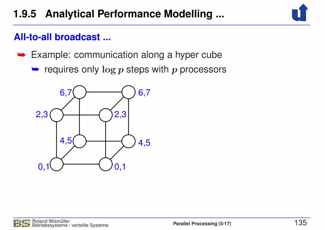
1.9.5 Analytical Performance Modelling ...
Roland WismullerBetriebssysteme / verteilte Systeme Parallel Processing (5/17) 135
All-to-all broadcast ...
➥ Example: communication along a hyper cube
➥ requires only log p steps with p processors
0,1
2,3
0,1
2,3
4,5 4,5
6,7 6,7
➥ Cost:
log p∑
i=1
(ts + 2i−1twm) = ts log p + twm(p− 1)
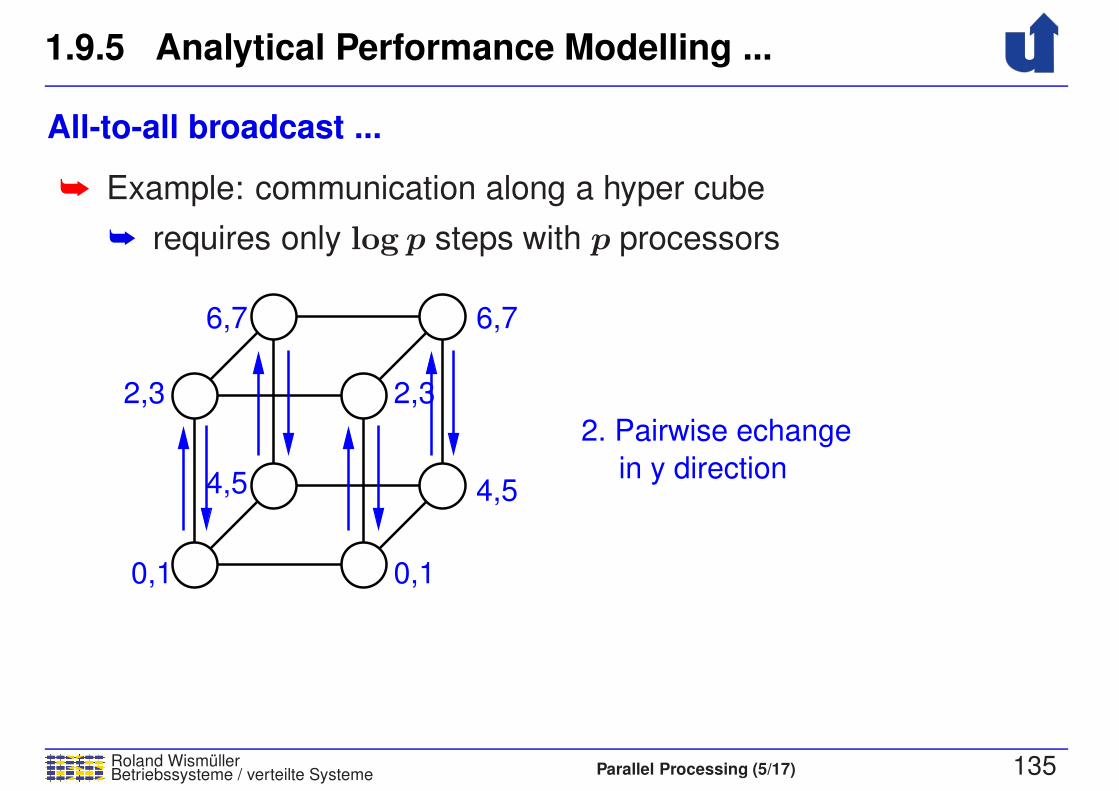
1.9.5 Analytical Performance Modelling ...
Roland WismullerBetriebssysteme / verteilte Systeme Parallel Processing (5/17) 135
All-to-all broadcast ...
➥ Example: communication along a hyper cube
➥ requires only log p steps with p processors
0,1
2,3
0,1
2,3
4,5 4,5
6,7 6,7
2. Pairwise echange
in y direction
➥ Cost:
log p∑
i=1
(ts + 2i−1twm) = ts log p + twm(p− 1)
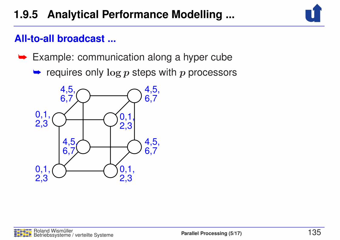
1.9.5 Analytical Performance Modelling ...
Roland WismullerBetriebssysteme / verteilte Systeme Parallel Processing (5/17) 135
All-to-all broadcast ...
➥ Example: communication along a hyper cube
➥ requires only log p steps with p processors
4,5,6,7
4,5,6,7
4,5,6,7
4,5,6,7
0,1,2,3
0,1,2,3
0,1,2,3
0,1,2,3
3. Pairwise echange
in z direction
➥ Cost:
log p∑
i=1
(ts + 2i−1twm) = ts log p + twm(p− 1)
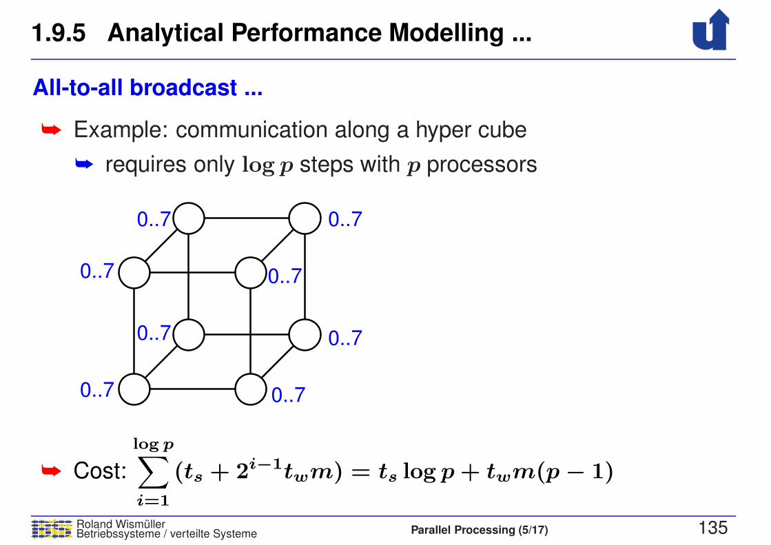
1.9.5 Analytical Performance Modelling ...
Roland WismullerBetriebssysteme / verteilte Systeme Parallel Processing (5/17) 135
All-to-all broadcast ...
➥ Example: communication along a hyper cube
➥ requires only log p steps with p processors
0..7
0..7
0..70..7
0..7
0..7
0..7
0..7
➥ Cost:
log p∑
i=1
(ts + 2i−1twm) = ts log p + twm(p− 1)

1.9.5 Analytical Performance Modelling ...
Roland WismullerBetriebssysteme / verteilte Systeme Parallel Processing (5/17) 136
All-to-all broadcast ...
Lab H−A 4111)
(Data from
t s
tw
= 71,5 µs
= 8,65 ns100000 Bytes
100 Bytes
Processors
Tim
e [m
s]
Hypercube
Ring
1000 Bytes
10000 Bytes
0 10 40 50 60
7
6
5
2
1
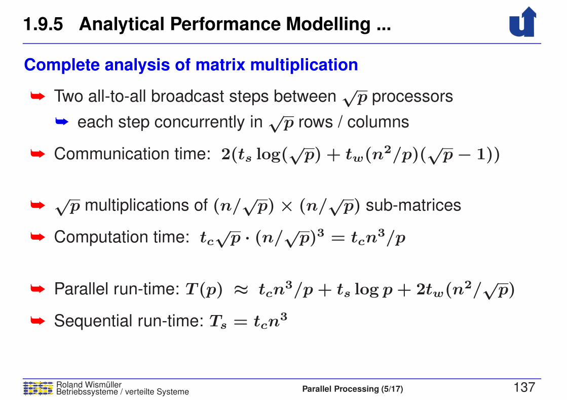
1.9.5 Analytical Performance Modelling ...
Roland WismullerBetriebssysteme / verteilte Systeme Parallel Processing (5/17) 137
Complete analysis of matrix multiplication
➥ Two all-to-all broadcast steps between√p processors
➥ each step concurrently in√p rows / columns
➥ Communication time: 2(ts log(√p) + tw(n2/p)(
√p− 1))
➥√p multiplications of (n/
√p)× (n/
√p) sub-matrices
➥ Computation time: tc√p · (n/√p)3 = tcn
3/p
➥ Parallel run-time: T (p) ≈ tcn3/p + ts log p + 2tw(n2/
√p)
➥ Sequential run-time: Ts = tcn3
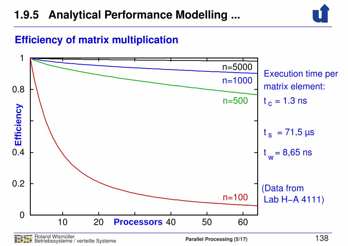
1.9.5 Analytical Performance Modelling ...
Roland WismullerBetriebssysteme / verteilte Systeme Parallel Processing (5/17) 138
Efficiency of matrix multiplication
Processors
Effi
cien
cy
matrix element:
Execution time per
Lab H−A 4111)
(Data from
t s
tw
= 71,5 µs
= 8,65 ns
n=5000
n=1000
n=500
n=100
t c = 1.3 ns
0.8
1
0.4
0.2
0 10 20 40 50 60
1.9.6 Performance Analysis Tools
Roland WismullerBetriebssysteme / verteilte Systeme Parallel Processing (5/17) 139
➥ Goal: performance debugging, i.e., finding and eliminating
performance bottlenecks
➥ Method: measurement of different quantities (metrics),
if applicable separated according to:
➥ execution unit (compute node, process, thread)
➥ source code position (procedure, source code line)
➥ time
➥ Tools are very different in their details
➥ method of measurement, required preparation steps,
processing of information, ...
➥ Some tools are also usable to visualise the program execution

1.9.6 Performance Analysis Tools ...
Roland WismullerBetriebssysteme / verteilte Systeme Parallel Processing (5/17) 140
Metrics for performance analysis
➥ CPU time (assessment of computing effort)
➥ Wall clock time (includes times where thread is blocked)
➥ Communication time and volume
➥ Metrics of the operating system:
➥ page faults, process switches, system calls, signals
➥ Hardware metrics (only with hardware support in the CPU):
➥ CPU cycles, floating point operations, memory accesses
➥ cache misses, cache invalidations, ...

1.9.6 Performance Analysis Tools ...
Roland WismullerBetriebssysteme / verteilte Systeme Parallel Processing (5/17) 141
Sampling (sample based performance analysis)
➥ Program is interrupted periodically
➥ Current value of the program counter is read (and maybe also the
call stack)
➥ The full measurement value is assigned to this place in the
program, e.g., when measuring CPU time:
➥ periodic interruption every 10ms CPU time
➥ CPU time[current PC value] += 10ms
➥ Mapping to source code level is done offline
➥ Result: measurement value for each function / source line

1.9.6 Performance Analysis Tools ...
Roland WismullerBetriebssysteme / verteilte Systeme Parallel Processing (5/17) 142
Profiling and tracing (event based performance analysis)
➥ Requires an instrumentation of the programs, e.g., insertion ofmeasurement code at interesting places
➥ often at the beginning and end of library routines, e.g.,MPI Recv, MPI Barrier, ...
➥ Tools usually do the instrumentation automatically
➥ typically, the program must be re-compiled or re-linked
➥ Analysis of the results is done during the measurement (profiling)or after the program execution (tracing)
➥ Result:
➥ measurement value for each measured function (profiling,tracing)
➥ development of the measurement value over time (tracing)
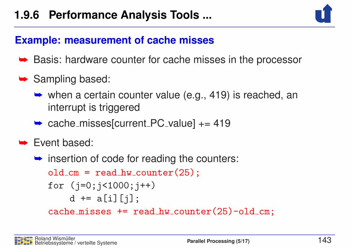
1.9.6 Performance Analysis Tools ...
Roland WismullerBetriebssysteme / verteilte Systeme Parallel Processing (5/17) 143
Example: measurement of cache misses
➥ Basis: hardware counter for cache misses in the processor
➥ Sampling based:
➥ when a certain counter value (e.g., 419) is reached, an
interrupt is triggered
➥ cache misses[current PC value] += 419
➥ Event based:
➥ insertion of code for reading the counters:
old cm = read hw counter(25);
for (j=0;j<1000;j++)
d += a[i][j];
cache misses += read hw counter(25)-old cm;

1.9.6 Performance Analysis Tools ...
Roland WismullerBetriebssysteme / verteilte Systeme Parallel Processing (5/17) 144
Pros and cons of the methods
➥ Sampling
➥ low and predictable overhead; reference to source code
➥ limited precision; no resolution in time
➥ Tracing
➥ acquisition of all relevant data with high resolution in time
➥ relatively high overhead; large volumes of data
➥ Profiling
➥ reduced volume of data, but less flexible
Roland WismullerBetriebssysteme / verteilte Systeme Parallel Processing (5/17) 145
Parallel ProcessingWS 2017/18
2 Parallel Programming with Shared Memory

2 Parallel Programming with Shared Memory ...
Roland WismullerBetriebssysteme / verteilte Systeme Parallel Processing (5/17) 146
Inhalt
➥ Basics
➥ Posix threads
➥ OpenMP basics
➥ Loop parallelization and dependeces
➥ OpenMP synchronization
➥ OpenMP details
Literature
➥ Wilkinson/Allen, Ch. 8.4, 8.5, Appendix C
➥ Hoffmann/Lienhart
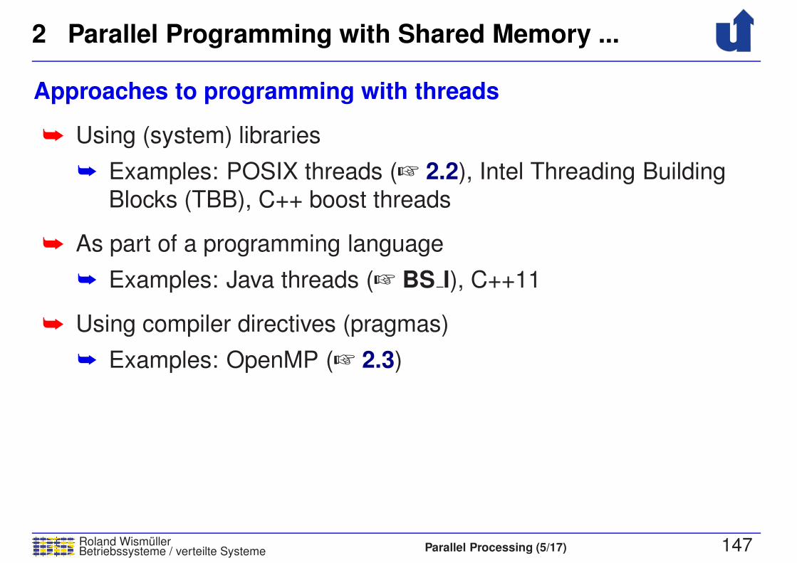
2 Parallel Programming with Shared Memory ...
Roland WismullerBetriebssysteme / verteilte Systeme Parallel Processing (5/17) 147
Approaches to programming with threads
➥ Using (system) libraries
➥ Examples: POSIX threads (☞ 2.2), Intel Threading Building
Blocks (TBB), C++ boost threads
➥ As part of a programming language
➥ Examples: Java threads (☞ BS I), C++11
➥ Using compiler directives (pragmas)
➥ Examples: OpenMP (☞ 2.3)

2.1 Basics
Roland WismullerBetriebssysteme / verteilte Systeme Parallel Processing (5/17) 148
2.1.1 Synchronization
➥ Ensuring conditions on the possible sequences of events in
threads
➥ mutual exclusion
➥ temporal order of actions in different threads
➥ Tools:
➥ shared variables
➥ semaphores / mutexes
➥ monitors / condition variables
➥ barriers

Roland WismullerBetriebssysteme / verteilte Systeme Parallel Processing (6/17) vii
Roland Wismuller
Universitat Siegen
Tel.: 0271/740-4050, Buro: H-B 8404
Stand: January 23, 2018
Parallel Processing
WS 2017/18
30.10.2017
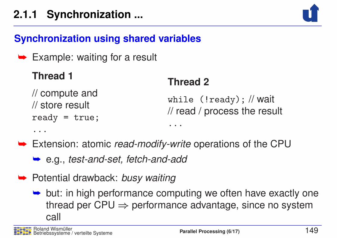
2.1.1 Synchronization ...
Roland WismullerBetriebssysteme / verteilte Systeme Parallel Processing (6/17) 149
Synchronization using shared variables
➥ Example: waiting for a result
Thread 1
// compute and
// store result
ready = true;
...
Thread 2
while (!ready); // wait
// read / process the result
...
➥ Extension: atomic read-modify-write operations of the CPU
➥ e.g., test-and-set, fetch-and-add
➥ Potential drawback: busy waiting
➥ but: in high performance computing we often have exactly one
thread per CPU⇒ performance advantage, since no system
call
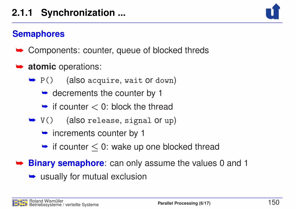
2.1.1 Synchronization ...
Roland WismullerBetriebssysteme / verteilte Systeme Parallel Processing (6/17) 150
Semaphores
➥ Components: counter, queue of blocked threds
➥ atomic operations:
➥ P() (also acquire, wait or down)
➥ decrements the counter by 1
➥ if counter < 0: block the thread
➥ V() (also release, signal or up)
➥ increments counter by 1
➥ if counter ≤ 0: wake up one blocked thread
➥ Binary semaphore: can only assume the values 0 and 1
➥ usually for mutual exclusion
2.1.1 Synchronization ...
Roland WismullerBetriebssysteme / verteilte Systeme Parallel Processing (6/17) 151
Monitors
➥ Module with data, procedures and initialization code
➥ access to data only via the monitor procedures
➥ (roughly corresponds to a class)
➥ All procedures are under mutual exclusion
➥ Further synchronization via condition variables
➥ two operations:
➥ wait(): blocks the calling thread
➥ signal(): wakes up some blocked threads
➥ variants: wake up only one thread / wake up all thread
➥ no “memory”: signal() only wakes a thread, if it already has
called wait() before
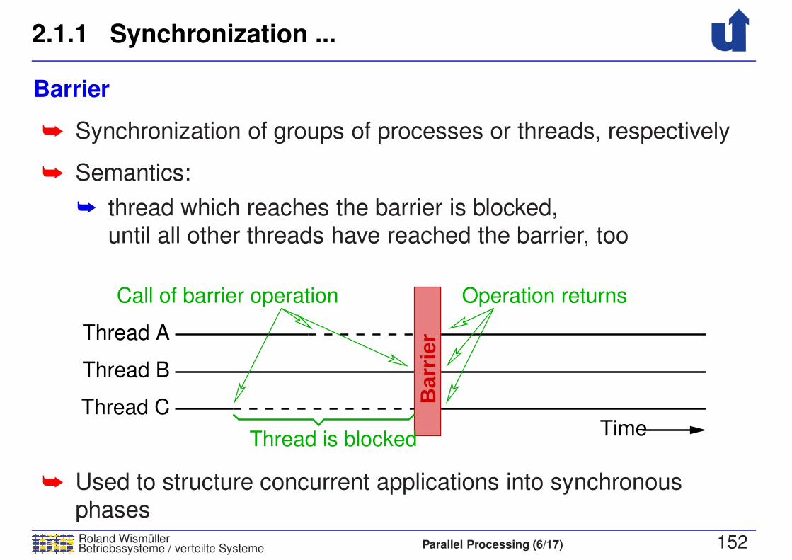
2.1.1 Synchronization ...
Roland WismullerBetriebssysteme / verteilte Systeme Parallel Processing (6/17) 152
Barrier
➥ Synchronization of groups of processes or threads, respectively
➥ Semantics:
➥ thread which reaches the barrier is blocked,until all other threads have reached the barrier, too
Thread A
Thread B
TimeB
arrie
rThread is blocked
Call of barrier operation Operation returns
Thread C
➥ Used to structure concurrent applications into synchronousphases

2.1 Basics ...
Roland WismullerBetriebssysteme / verteilte Systeme Parallel Processing (6/17) 153
2.1.2 Synchronization errors
➥ Insufficiend synchronization: race conditions
➥ result of the calculation is different (or false), depending on
temporal interleaving of the threads
➥ important: do not assume FIFO semantics of the queues in
synchronization constructs!
➥ Deadlocks
➥ a group of threads waits for conditions, which can only be
fulfilled by the other threads in this group
➥ Starvation (unfairness)
➥ a thread waiting for a condition can never execute, although
the condition is fulfilled regularly
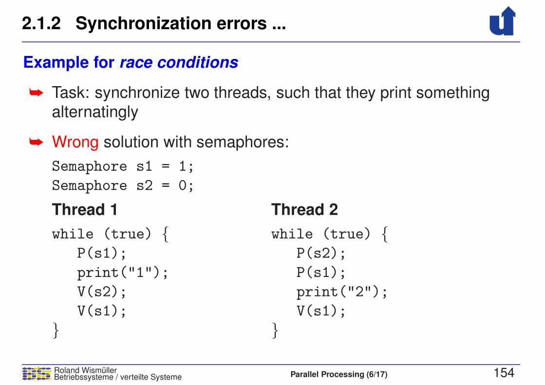
2.1.2 Synchronization errors ...
Roland WismullerBetriebssysteme / verteilte Systeme Parallel Processing (6/17) 154
Example for race conditions
➥ Task: synchronize two threads, such that they print something
alternatingly
➥ Wrong solution with semaphores:
Semaphore s1 = 1;
Semaphore s2 = 0;
Thread 1
while (true) {P(s1);
print("1");
V(s2);
V(s1);
}
Thread 2
while (true) {P(s2);
P(s1);
print("2");
V(s1);
}
2.1 Basics ...
Roland WismullerBetriebssysteme / verteilte Systeme Parallel Processing (6/17) 155
2.1.3 Lock-Free and Wait-Free Data Structures
➥ Goal: Data structures (typically collections) without mutual
exclusion
➥ more performant, no danger of deadlocks
➥ Lock-free: under any circumstances at least one of the threads
makes progress after a finite number of steps
➥ in addition, wait-free also prevents starvation
➥ Typical approach:
➥ use atomic read-modify-write instrcutions instead of locks
➥ in case of conflict, i.e., when there is a simultaneous change
by another thread, the affected operation is repeated
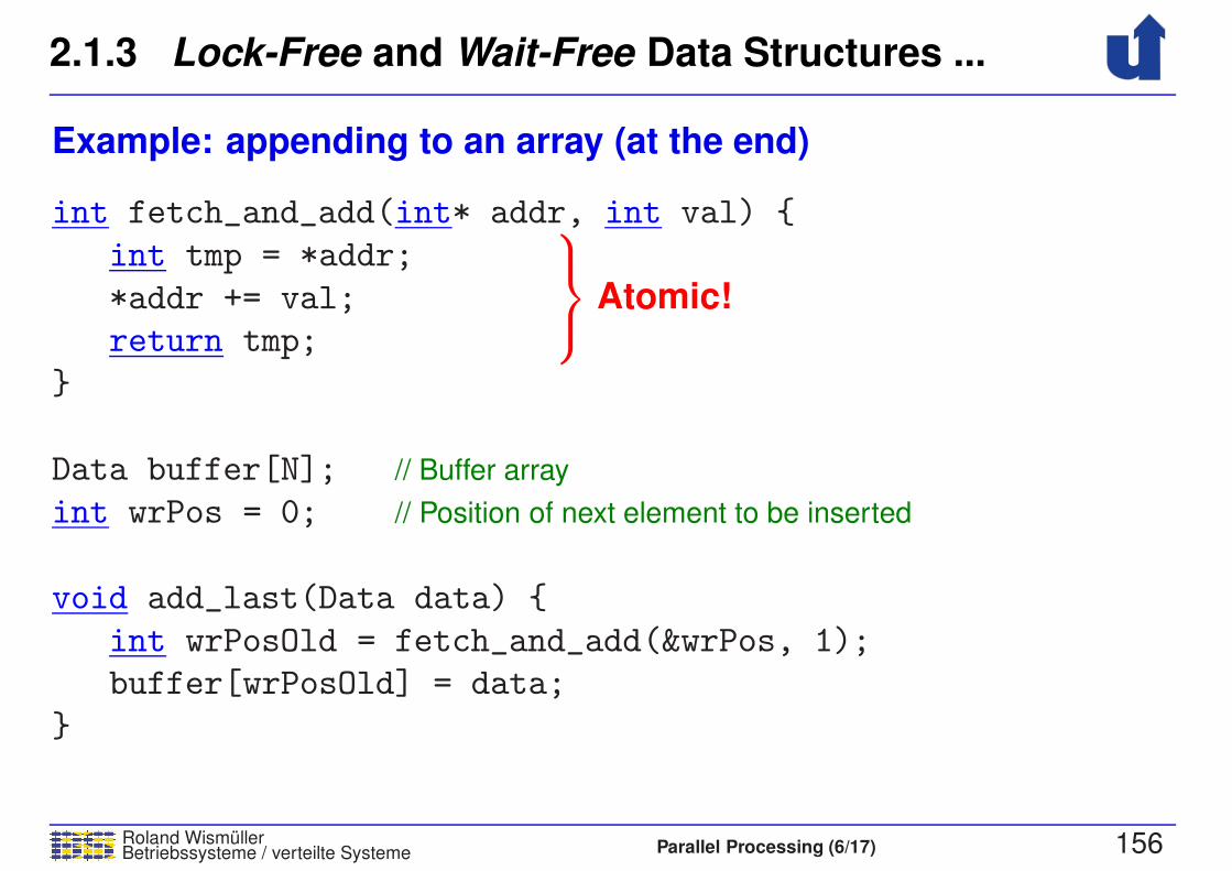
2.1.3 Lock-Free and Wait-Free Data Structures ...
Roland WismullerBetriebssysteme / verteilte Systeme Parallel Processing (6/17) 156
Example: appending to an array (at the end)
int fetch_and_add(int* addr, int val) {
int tmp = *addr;
*addr += val;
return tmp;
}
Data buffer[N]; // Buffer array
int wrPos = 0; // Position of next element to be inserted
void add_last(Data data) {
int wrPosOld = fetch_and_add(&wrPos, 1);
buffer[wrPosOld] = data;
}
Atomic!
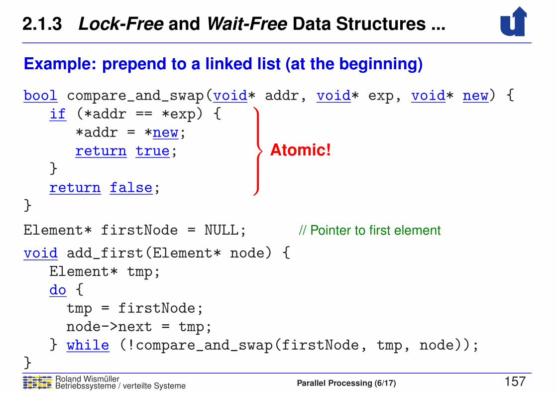
2.1.3 Lock-Free and Wait-Free Data Structures ...
Roland WismullerBetriebssysteme / verteilte Systeme Parallel Processing (6/17) 157
Example: prepend to a linked list (at the beginning)
bool compare_and_swap(void* addr, void* exp, void* new) {if (*addr == *exp) {
*addr = *new;return true;
}return false;
}
Element* firstNode = NULL; // Pointer to first element
void add_first(Element* node) {Element* tmp;do {tmp = firstNode;node->next = tmp;
} while (!compare_and_swap(firstNode, tmp, node));}
Atomic!

2.1.3 Lock-Free and Wait-Free Data Structures ...
Roland WismullerBetriebssysteme / verteilte Systeme Parallel Processing (6/17) 158
➥ Problems
➥ re-use of memory addresses can result in corrupt data
structures
➥ assumption in linked list: if firstNode is still unchanged,
the list was not accessed concurrently
➥ thus, we need special procedures for memory deallocation
➥ There is a number of libraries for C++ and also for Java
➥ C++: e.g., boost.lockfree, libcds, Concurrency Kit, liblfds
➥ Java: e.g., Amino Concurrent Building Blocks, Highly Scalable
Java
➥ Compilers usually offer read-modify-write operations
➥ e.g., gcc/g++: built-in functions __sync_...()

2.2 POSIX Threads (PThreads)
Roland WismullerBetriebssysteme / verteilte Systeme Parallel Processing (6/17) 159
➥ IEEE 1003.1c: standard interface for programming with threads
➥ implemented by a system library
➥ (mostly) independent of operating system
➥ Programming model:
➥ at program start: exactly one (master) thread
➥ master thread creates other threads
and should usualy wait for them to finish
➥ process terminates when master thread terminates
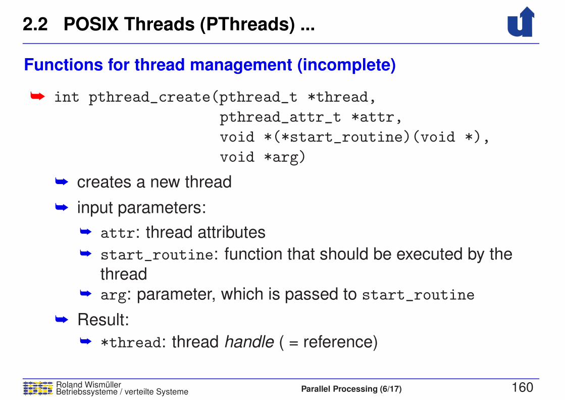
2.2 POSIX Threads (PThreads) ...
Roland WismullerBetriebssysteme / verteilte Systeme Parallel Processing (6/17) 160
Functions for thread management (incomplete)
➥ int pthread_create(pthread_t *thread,
pthread_attr_t *attr,
void *(*start_routine)(void *),
void *arg)
➥ creates a new thread
➥ input parameters:
➥ attr: thread attributes
➥ start_routine: function that should be executed by the
thread➥ arg: parameter, which is passed to start_routine
➥ Result:
➥ *thread: thread handle ( = reference)
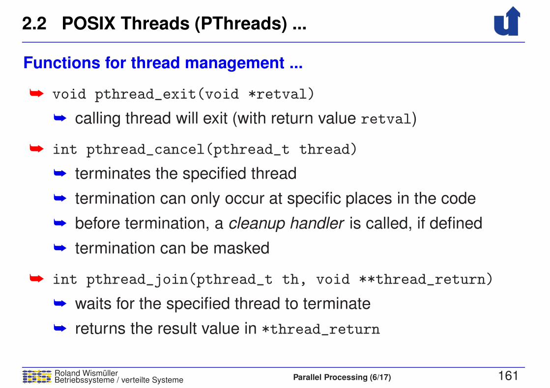
2.2 POSIX Threads (PThreads) ...
Roland WismullerBetriebssysteme / verteilte Systeme Parallel Processing (6/17) 161
Functions for thread management ...
➥ void pthread_exit(void *retval)
➥ calling thread will exit (with return value retval)
➥ int pthread_cancel(pthread_t thread)
➥ terminates the specified thread
➥ termination can only occur at specific places in the code
➥ before termination, a cleanup handler is called, if defined
➥ termination can be masked
➥ int pthread_join(pthread_t th, void **thread_return)
➥ waits for the specified thread to terminate
➥ returns the result value in *thread_return
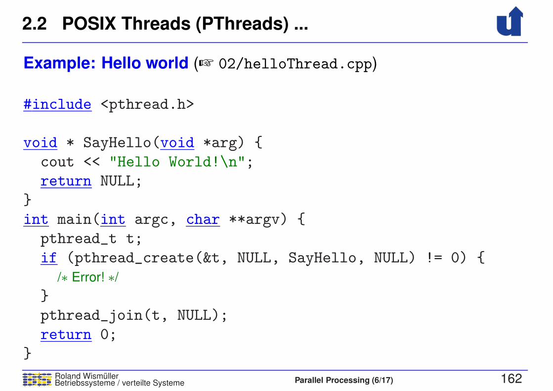
2.2 POSIX Threads (PThreads) ...
Roland WismullerBetriebssysteme / verteilte Systeme Parallel Processing (6/17) 162
Example: Hello world (☞ 02/helloThread.cpp)
#include <pthread.h>
void * SayHello(void *arg) {
cout << "Hello World!\n";
return NULL;
}
int main(int argc, char **argv) {
pthread_t t;
if (pthread_create(&t, NULL, SayHello, NULL) != 0) {
/∗ Error! ∗/
}
pthread_join(t, NULL);
return 0;
}
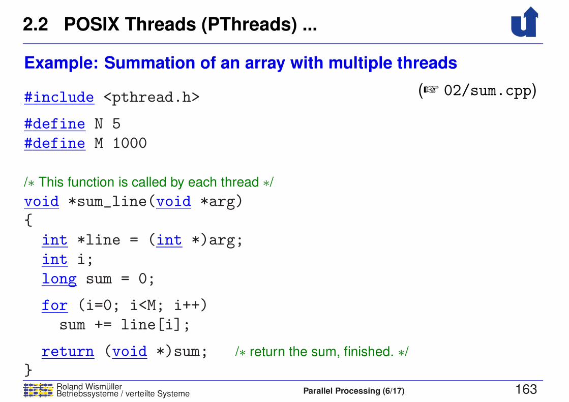
2.2 POSIX Threads (PThreads) ...
Roland WismullerBetriebssysteme / verteilte Systeme Parallel Processing (6/17) 163
Example: Summation of an array with multiple threads
(☞ 02/sum.cpp)#include <pthread.h>
#define N 5
#define M 1000
/∗ This function is called by each thread ∗/
void *sum_line(void *arg){
int *line = (int *)arg;int i;
long sum = 0;
for (i=0; i<M; i++)
sum += line[i];
return (void *)sum; /∗ return the sum, finished. ∗/
}
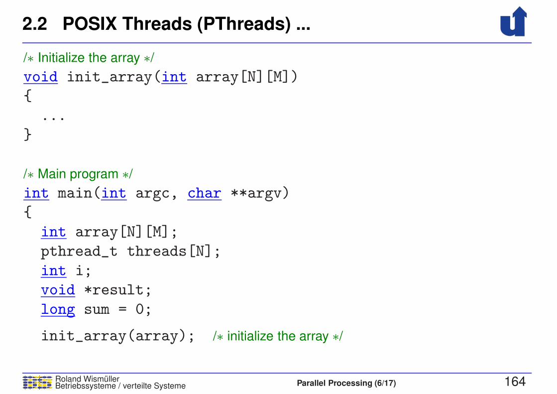
2.2 POSIX Threads (PThreads) ...
Roland WismullerBetriebssysteme / verteilte Systeme Parallel Processing (6/17) 164
/∗ Initialize the array ∗/
void init_array(int array[N][M])
{
...
}
/∗ Main program ∗/
int main(int argc, char **argv)
{
int array[N][M];
pthread_t threads[N];
int i;
void *result;
long sum = 0;
init_array(array); /∗ initialize the array ∗/

2.2 POSIX Threads (PThreads) ...
Roland WismullerBetriebssysteme / verteilte Systeme Parallel Processing (6/17) 165
/∗ Create a thread for each line, with a pointer to the line as parameter ∗/
/∗ Caution: error checks and thread attributes are missing! ∗/
for (i=0; i<N; i++) {
pthread_create(&threads[i], NULL, sum_line, array[i]);
}
/∗ Wait for termination, sum up the results ∗/
for (i=0; i<N; i++) {
pthread_join(threads[i], &result);
sum += (long)result;
}
cout << "Sum: " << sum << "\n";
}
Compile and link the program
➥ g++ -o sum sum.cpp -pthread

2.2 POSIX Threads (PThreads) ...
Roland WismullerBetriebssysteme / verteilte Systeme Parallel Processing (6/17) 166
Remarks on the example
➥ PThreads only allows to pass one argument
➥ usually, a pointer to an argument data structure
➥ pointer to a local variable is only allowed, if pthread_join
is called within the same procedure!
➥ The return value of a thread is void *
➥ ugly type conversion
➥ with multiple return values: pointer to a data structure
(allocated globally or dynamically)
➥ No synchronization is required
➥ pthread_join can only wait for a specific thread
➥ inefficient, when threads have different execution times
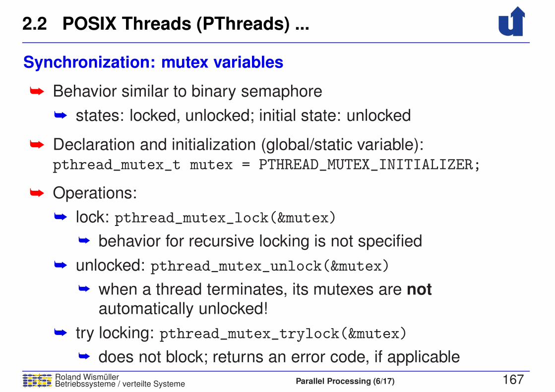
2.2 POSIX Threads (PThreads) ...
Roland WismullerBetriebssysteme / verteilte Systeme Parallel Processing (6/17) 167
Synchronization: mutex variables
➥ Behavior similar to binary semaphore
➥ states: locked, unlocked; initial state: unlocked
➥ Declaration and initialization (global/static variable):pthread_mutex_t mutex = PTHREAD_MUTEX_INITIALIZER;
➥ Operations:
➥ lock: pthread_mutex_lock(&mutex)
➥ behavior for recursive locking is not specified
➥ unlocked: pthread_mutex_unlock(&mutex)
➥ when a thread terminates, its mutexes are notautomatically unlocked!
➥ try locking: pthread_mutex_trylock(&mutex)
➥ does not block; returns an error code, if applicable

2.2 POSIX Threads (PThreads) ...
Roland WismullerBetriebssysteme / verteilte Systeme Parallel Processing (6/17) 168
Synchronization: condition variables
➥ Declaration and initialization (global/static variable):pthread_cond_t cond = PTHREAD_COND_INITIALIZER;
➥ Operations:
➥ wait: pthread_cond_wait(&cond, &mutex)
➥ thread is blocked, mutex will be unlocked temporarily
➥ signaling thread keeps the mutex, i.e., the condition may nolonger be fulfilled when the routine returns!
➥ typical use:
while (!condition_met)pthread_cond_wait(&cond, &mutex);
➥ signal:
➥ to a single thread: pthread_cond_signal(&cond)
➥ to all threads: pthread_cond_broadcast(&cond)
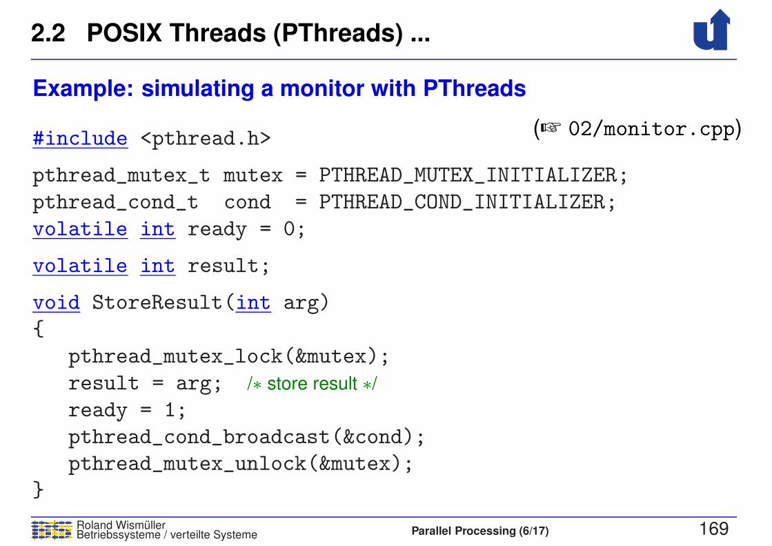
2.2 POSIX Threads (PThreads) ...
Roland WismullerBetriebssysteme / verteilte Systeme Parallel Processing (6/17) 169
Example: simulating a monitor with PThreads
(☞ 02/monitor.cpp)#include <pthread.h>
pthread_mutex_t mutex = PTHREAD_MUTEX_INITIALIZER;
pthread_cond_t cond = PTHREAD_COND_INITIALIZER;
volatile int ready = 0;
volatile int result;
void StoreResult(int arg)
{
pthread_mutex_lock(&mutex);
result = arg; /∗ store result ∗/
ready = 1;
pthread_cond_broadcast(&cond);
pthread_mutex_unlock(&mutex);
}

2.2 POSIX Threads (PThreads) ...
Roland WismullerBetriebssysteme / verteilte Systeme Parallel Processing (6/17) 170
Example: simulating a monitor with PThreads ...
int ReadResult(){
int tmp;pthread_mutex_lock(&mutex);while (ready != 1)
pthread_cond_wait(&cond, &mutex);tmp = result; /∗ read result ∗/
pthread_mutex_unlock(&mutex);return tmp;
}
➥ while is important, since the waiting thread unlocks the mutex
➥ another thread could destroy the condition again before thewaiting thread regains the mutex
(although this cannot happen in this concrete example!)
2.3 OpenMP Basics
Roland WismullerBetriebssysteme / verteilte Systeme Parallel Processing (6/17) 171
Background
➥ Thread libraries (for FORTRAN and C) are often too complex(and partially system dependent) for application programmers
➥ wish: more abstract, portable constructs
➥ OpenMP is an inofficial standard
➥ since 1997 by the OpenMP forum (www.openmp.org)
➥ API for parallel programming with shared memory usingFORTRAN / C / C++
➥ source code directives
➥ library routines
➥ environment variables
➥ Besides parallel processing with threads, OpenMP also supportsSIMD extensions and external accelerators (since version 4.0)

Roland WismullerBetriebssysteme / verteilte Systeme Parallel Processing (7/17) viii
Roland Wismuller
Universitat Siegen
Tel.: 0271/740-4050, Buro: H-B 8404
Stand: January 23, 2018
Parallel Processing
WS 2017/18
06.11.2017
2.3 OpenMP Basics ...
Roland WismullerBetriebssysteme / verteilte Systeme Parallel Processing (7/17) 172
Parallelization using directives
➥ The programmer must specify
➥ which code regions should be executed in parallel
➥ where a synchronization is necessary
➥ This specification is done using directives (pragmas)
➥ special control statements for the compiler
➥ unknown directives are ignored by the compiler
➥ Thus, a program with OpenMP directives can be compiled
➥ with an OpenMP compiler, resulting in a parallel program
➥ with a standard compiler, resulting in a sequential program

2.3 OpenMP Basics ...
Roland WismullerBetriebssysteme / verteilte Systeme Parallel Processing (7/17) 173
Parallelization using directives ...
➥ Goal of parallelizing with OpenMP:
➥ distribute the execution of sequential program code to several
threads, without changing the code
➥ identical source code for sequential and parallel version
➥ Three main classes of directives:
➥ directives for creating threads (parallel, parallel region)
➥ within a parallel region: directives to distribute the work to the
individual threads
➥ data parallelism: distribution of loop iterations (for)
➥ task parallelism: parallel code regions (sections) and
explicit tasks (task)
➥ directives for synchronization
2.3 OpenMP Basics ...
Roland WismullerBetriebssysteme / verteilte Systeme Parallel Processing (7/17) 174
Parallelization using directives: discussion
➥ Compromise between
➥ completely manual parallelization (as, e.g., with MPI)
➥ automatic parallelization by the compiler
➥ Compiler takes over the organization of the parallel tasks
➥ thread creation, distribution of tasks, ...
➥ Programmer takes over the necessary dependence analysis
➥ which code regions can be executed in parallel?
➥ enables detailed control over parallelism
➥ but: programmer is responsible for correctness
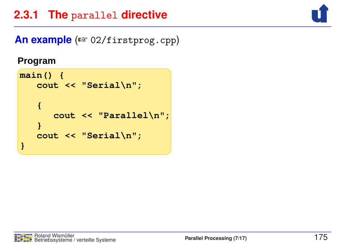
2.3.1 The parallel directive
Roland WismullerBetriebssysteme / verteilte Systeme Parallel Processing (7/17) 175
An example (☞ 02/firstprog.cpp)
Program
main() {
{
}
}
cout << "Serial\n";
cout << "Parallel\n";
cout << "Serial\n";
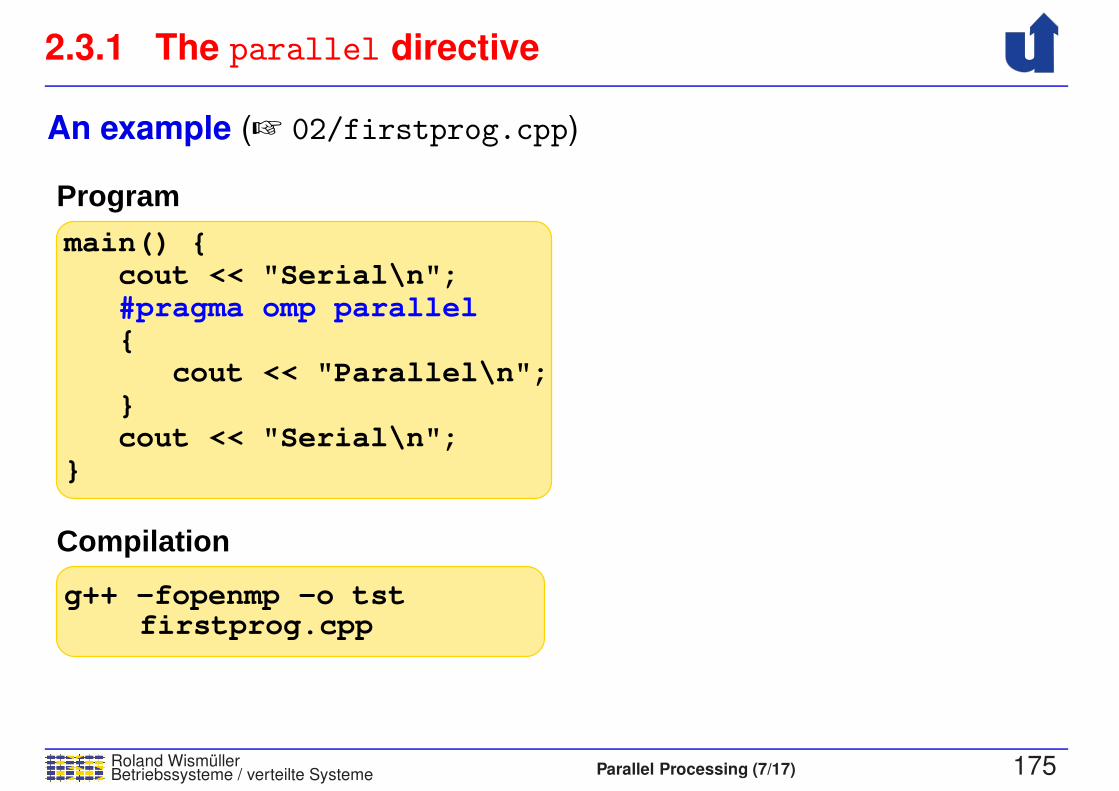
2.3.1 The parallel directive
Roland WismullerBetriebssysteme / verteilte Systeme Parallel Processing (7/17) 175
An example (☞ 02/firstprog.cpp)
Program
main() {
{
}
}
cout << "Serial\n";
cout << "Parallel\n";
cout << "Serial\n";
#pragma omp parallel
Compilation
firstprog.cppg++ −fopenmp −o tst
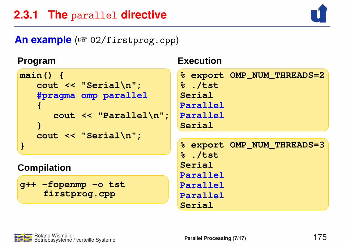
2.3.1 The parallel directive
Roland WismullerBetriebssysteme / verteilte Systeme Parallel Processing (7/17) 175
An example (☞ 02/firstprog.cpp)
Program
main() {
{
}
}
cout << "Serial\n";
cout << "Parallel\n";
cout << "Serial\n";
#pragma omp parallel
Compilation
firstprog.cppg++ −fopenmp −o tst
Execution
SerialParallelParallelParallelSerial% ./tst% export OMP_NUM_THREADS=3
SerialParallelParallelSerial% ./tst% export OMP_NUM_THREADS=2
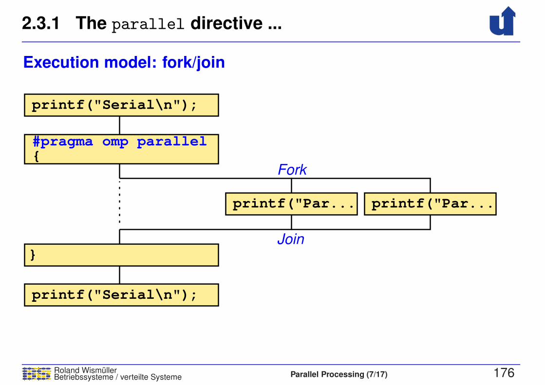
2.3.1 The parallel directive ...
Roland WismullerBetriebssysteme / verteilte Systeme Parallel Processing (7/17) 176
Execution model: fork/join
Fork
Join
#pragma omp parallel{
printf("Serial\n");
}
printf("Serial\n");
printf("Par... printf("Par...
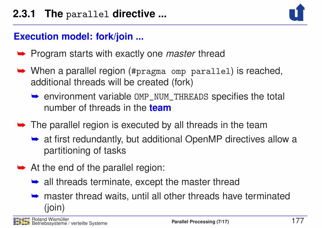
2.3.1 The parallel directive ...
Roland WismullerBetriebssysteme / verteilte Systeme Parallel Processing (7/17) 177
Execution model: fork/join ...
➥ Program starts with exactly one master thread
➥ When a parallel region (#pragma omp parallel) is reached,additional threads will be created (fork)
➥ environment variable OMP_NUM_THREADS specifies the totalnumber of threads in the team
➥ The parallel region is executed by all threads in the team
➥ at first redundantly, but additional OpenMP directives allow apartitioning of tasks
➥ At the end of the parallel region:
➥ all threads terminate, except the master thread
➥ master thread waits, until all other threads have terminated(join)
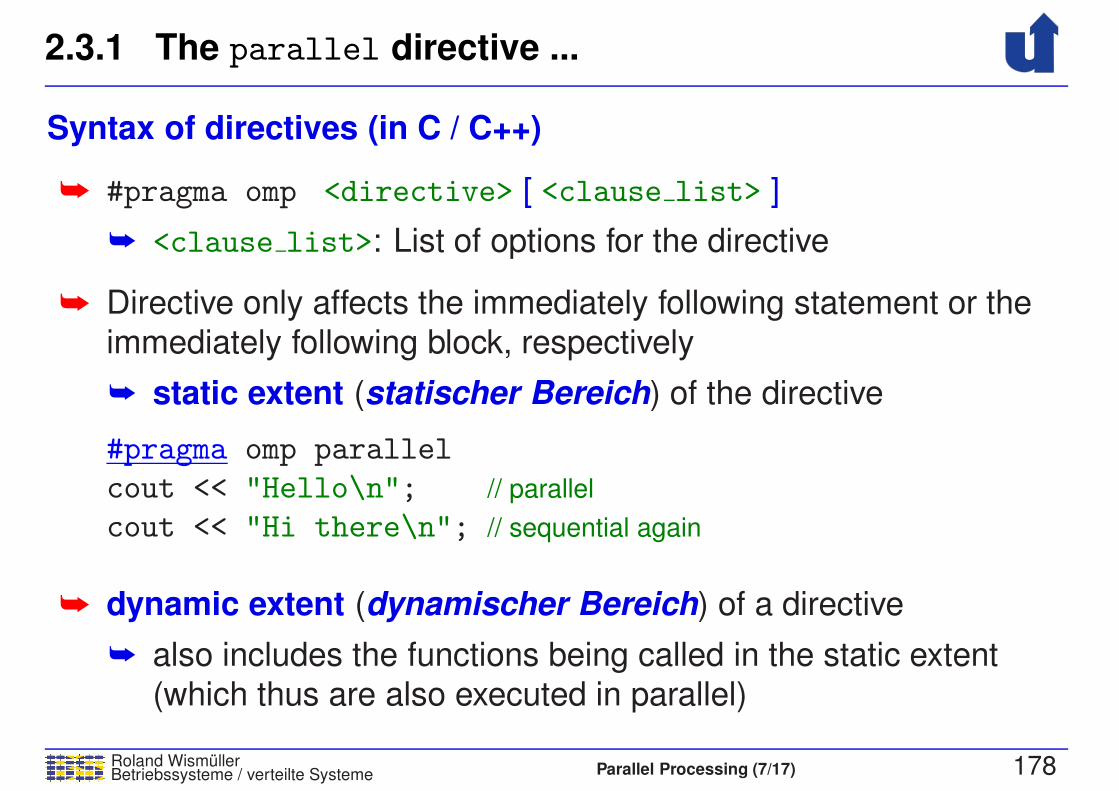
2.3.1 The parallel directive ...
Roland WismullerBetriebssysteme / verteilte Systeme Parallel Processing (7/17) 178
Syntax of directives (in C / C++)
➥ #pragma omp <directive> [ <clause list> ]
➥ <clause list>: List of options for the directive
➥ Directive only affects the immediately following statement or the
immediately following block, respectively
➥ static extent (statischer Bereich) of the directive
#pragma omp parallel
cout << "Hello\n"; // parallel
cout << "Hi there\n"; // sequential again
➥ dynamic extent (dynamischer Bereich) of a directive
➥ also includes the functions being called in the static extent
(which thus are also executed in parallel)
2.3.1 The parallel directive ...
Roland WismullerBetriebssysteme / verteilte Systeme Parallel Processing (7/17) 179
Shared and private variables
➥ For variables in a parallel region there are two alternatives
➥ the variables is shared by all threads (shared variable)
➥ all threads access the same variable➥ usually, some synchronization is required!
➥ each thread has its own private instance (private variable)
➥ can be initialized with the value in the master thread
➥ value is dropped at the end of the parallel region
➥ For variables, which are declared within the dynamic extent of a
parallel directive, the following holds:
➥ local variables are private
➥ static variables and heap variables (new) are shared
2.3.1 The parallel directive ...
Roland WismullerBetriebssysteme / verteilte Systeme Parallel Processing (7/17) 180
Shared and private variables ...
➥ For variables, which have been declared before entering a
parallel region, the behavior can be specified by an option of the
parallel directive:
➥ private ( <variable list> )
➥ private variable, without initialization
➥ firstprivate ( <variable list> )
➥ private variable
➥ initialized with the value in the master thread
➥ shared ( <variable list> )
➥ shared variable
➥ shared is the default for all variables
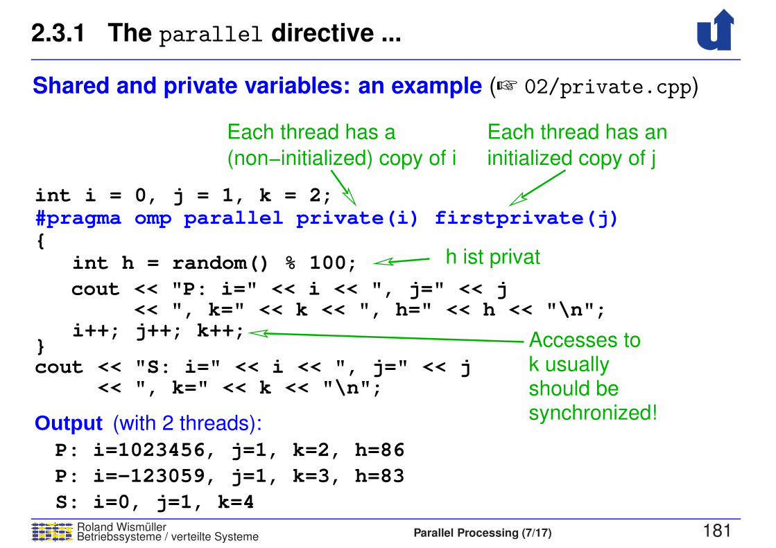
2.3.1 The parallel directive ...
Roland WismullerBetriebssysteme / verteilte Systeme Parallel Processing (7/17) 181
Shared and private variables: an example (☞ 02/private.cpp)
int i = 0, j = 1, k = 2;#pragma omp parallel private(i) firstprivate(j){ int h = random() % 100;
<< ", k=" << k << "\n";
}
cout << "P: i=" << i << ", j=" << j<< ", k=" << k << ", h=" << h << "\n";
i++; j++; k++;
cout << "S: i=" << i << ", j=" << j
OutputP: i=1023456, j=1, k=2, h=86
P: i=−123059, j=1, k=3, h=83
S: i=0, j=1, k=4
(with 2 threads):
Accesses tok usuallyshould besynchronized!
(non−initialized) copy of i
h ist privat
Each thread has an
initialized copy of j
Each thread has a
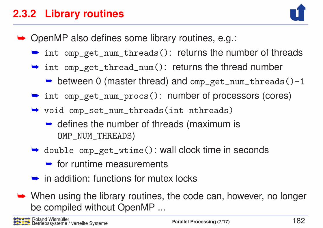
2.3.2 Library routines
Roland WismullerBetriebssysteme / verteilte Systeme Parallel Processing (7/17) 182
➥ OpenMP also defines some library routines, e.g.:
➥ int omp_get_num_threads(): returns the number of threads
➥ int omp_get_thread_num(): returns the thread number
➥ between 0 (master thread) and omp_get_num_threads()-1
➥ int omp_get_num_procs(): number of processors (cores)
➥ void omp_set_num_threads(int nthreads)
➥ defines the number of threads (maximum is
OMP_NUM_THREADS)
➥ double omp_get_wtime(): wall clock time in seconds
➥ for runtime measurements
➥ in addition: functions for mutex locks
➥ When using the library routines, the code can, however, no longerbe compiled without OpenMP ...
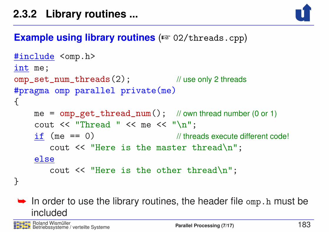
2.3.2 Library routines ...
Roland WismullerBetriebssysteme / verteilte Systeme Parallel Processing (7/17) 183
Example using library routines (☞ 02/threads.cpp)
#include <omp.h>
int me;
omp_set_num_threads(2); // use only 2 threads
#pragma omp parallel private(me)
{
me = omp_get_thread_num(); // own thread number (0 or 1)
cout << "Thread " << me << "\n";
if (me == 0) // threads execute different code!
cout << "Here is the master thread\n";
else
cout << "Here is the other thread\n";
}
➥ In order to use the library routines, the header file omp.h must be
included
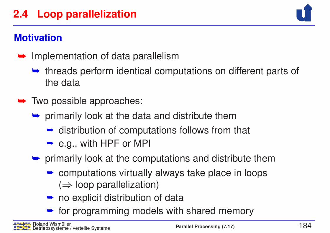
2.4 Loop parallelization
Roland WismullerBetriebssysteme / verteilte Systeme Parallel Processing (7/17) 184
Motivation
➥ Implementation of data parallelism
➥ threads perform identical computations on different parts of
the data
➥ Two possible approaches:
➥ primarily look at the data and distribute them
➥ distribution of computations follows from that
➥ e.g., with HPF or MPI
➥ primarily look at the computations and distribute them
➥ computations virtually always take place in loops
(⇒ loop parallelization)
➥ no explicit distribution of data
➥ for programming models with shared memory
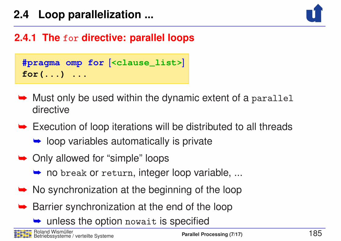
2.4 Loop parallelization ...
Roland WismullerBetriebssysteme / verteilte Systeme Parallel Processing (7/17) 185
2.4.1 The for directive: parallel loops
#pragma omp for
for(...) ...
<clause_list>][
➥ Must only be used within the dynamic extent of a parallel
directive
➥ Execution of loop iterations will be distributed to all threads
➥ loop variables automatically is private
➥ Only allowed for “simple” loops
➥ no break or return, integer loop variable, ...
➥ No synchronization at the beginning of the loop
➥ Barrier synchronization at the end of the loop
➥ unless the option nowait is specified
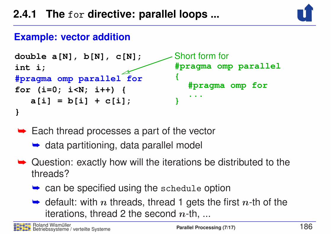
2.4.1 The for directive: parallel loops ...
Roland WismullerBetriebssysteme / verteilte Systeme Parallel Processing (7/17) 186
Example: vector addition
for (i=0; i<N; i++) {
a[i] = b[i] + c[i];
double a[N], b[N], c[N];
int i;
#pragma omp parallel for
}
#pragma omp parallelShort form for
{#pragma omp for...
}
➥ Each thread processes a part of the vector
➥ data partitioning, data parallel model
➥ Question: exactly how will the iterations be distributed to thethreads?
➥ can be specified using the schedule option
➥ default: with n threads, thread 1 gets the first n-th of theiterations, thread 2 the second n-th, ...
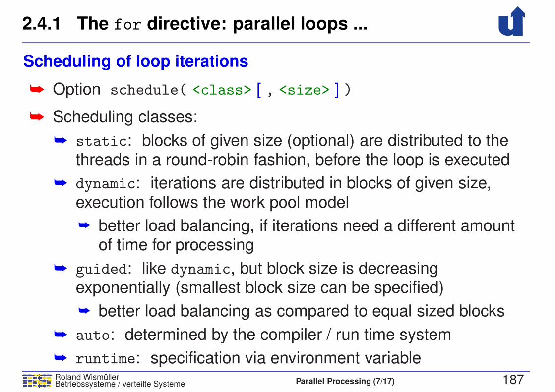
2.4.1 The for directive: parallel loops ...
Roland WismullerBetriebssysteme / verteilte Systeme Parallel Processing (7/17) 187
Scheduling of loop iterations
➥ Option schedule( <class> [ , <size> ] )
➥ Scheduling classes:
➥ static: blocks of given size (optional) are distributed to thethreads in a round-robin fashion, before the loop is executed
➥ dynamic: iterations are distributed in blocks of given size,execution follows the work pool model
➥ better load balancing, if iterations need a different amountof time for processing
➥ guided: like dynamic, but block size is decreasingexponentially (smallest block size can be specified)
➥ better load balancing as compared to equal sized blocks
➥ auto: determined by the compiler / run time system
➥ runtime: specification via environment variable

2.4.1 The for directive: parallel loops ...
Roland WismullerBetriebssysteme / verteilte Systeme Parallel Processing (7/17) 188
Scheduling example(☞ 02/loops.cpp)
int i, j;
double x;
#pragma omp parallel for private(i,j,x) schedule(runtime)
for (i=0; i<40000; i++) {
x = 1.2;
for (j=0; j<i; j++) { // triangular loop
x = sqrt(x) * sin(x*x);
}
}
➥ Scheduling can be specified at runtime, e.g.:
➥ export OMP_SCHEDULE="static,10"
➥ Useful for optimization experiments

2.4.1 The for directive: parallel loops ...
Roland WismullerBetriebssysteme / verteilte Systeme Parallel Processing (7/17) 189
Scheduling example: results
➥ Runtime with 4 threads on the lab computers:
OMP SCHEDULE "static" "static,1" "dynamic" "guided"
Time 3.1 s 1.9 s 1.8 s 1.8 s
➥ Load imbalance when using "static"
➥ thread 1: i=0..9999, thread 4: i=30000..39999
➥ "static,1" and "dynamic" use a block size of 1
➥ each thread executes every 4th iteration of the i loop
➥ can be very inefficient due to caches (false sharing, ☞ 4.1)
➥ remedy: use larger block size (e.g.: "dynamic,100")
➥ "guided" often is a good compromize between load balancing
and locality (cache usage)

2.4.1 The for directive: parallel loops ...
Roland WismullerBetriebssysteme / verteilte Systeme Parallel Processing (7/17) 190
Shared and private variables in loops
➥ The for directive can be supplemented with the options private,shared and firstprivate (see slide 179 ff.)
➥ In addition, there is an option lastprivate
➥ private variable
➥ after the loop, the master thread has the value of the lastiteration
➥ Example:
int i = 0;
#pragma omp parallel for lastprivate(i)
for (i=0; i<100; i++) {
...
}
printf("i=%d\\n",i); // prints the value 100

2.4.2 Parallelization of Loops
Roland WismullerBetriebssysteme / verteilte Systeme Parallel Processing (7/17) 191
When can a loop be parallelized?
for(i=1;i<N;i++)
a[i] = a[i]+ b[i−1];
for(i=1;i<N;i++)
a[i] = a[i−1]+ b[i];
for(i=0;i<N;i++)
a[i] = a[i+1]+ b[i];
➥ Optimal: independent loops (forall loop)
➥ loop iterations can be executed concurrently without any
synchronization
➥ there must not be any dependeces between statements in
different loop iterations
➥ (equivalent: the statements in different iterations must fulfill the
Bernstein conditions)
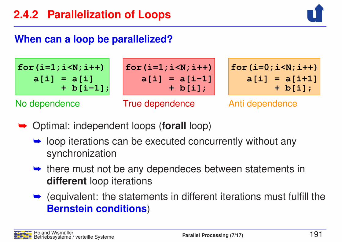
2.4.2 Parallelization of Loops
Roland WismullerBetriebssysteme / verteilte Systeme Parallel Processing (7/17) 191
When can a loop be parallelized?
No dependence True dependence Anti dependence
for(i=1;i<N;i++)
a[i] = a[i]+ b[i−1];
for(i=1;i<N;i++)
a[i] = a[i−1]+ b[i];
for(i=0;i<N;i++)
a[i] = a[i+1]+ b[i];
➥ Optimal: independent loops (forall loop)
➥ loop iterations can be executed concurrently without any
synchronization
➥ there must not be any dependeces between statements in
different loop iterations
➥ (equivalent: the statements in different iterations must fulfill the
Bernstein conditions)

2.4.2 Parallelization of Loops ...
Roland WismullerBetriebssysteme / verteilte Systeme Parallel Processing (7/17) 192
Handling of data dependences in loops
➥ Anti and output dependences:
➥ can always be removed, e.g., by consistent renaming of
variables
➥ in the previous example:
{#pragma omp parallel
#pragma omp for
for(i=1;i<=N;i++)
#pragma omp for
a2[i] = a[i];
for(i=0;i<N;i++)a[i] = a2[i+1] + b[i];
}
➥ the barrier at the end of the first loop is necessary!

2.4.2 Parallelization of Loops ...
Roland WismullerBetriebssysteme / verteilte Systeme Parallel Processing (7/17) 193
Handling of data dependences in loops ...
➥ True dependence:
➥ introduce proper synchronization between the threads
➥ e.g., using the ordered directive (☞ 2.6):
#pragma omp parallel for orderedfor (i=1;i<N;i++) {
// long computation of b[i]
#pragma omp ordereda[i] = a[i-1] + b[i];
}
➥ disadvantage: degree of parallelism often is largely reduced
➥ sometimes, a vectorization (SIMD) is possible (☞ 2.8.2), e.g.:
#pragma omp simd safelen(4)for (i=4;i<N;i++)
a[i] = a[i-4] + b[i];
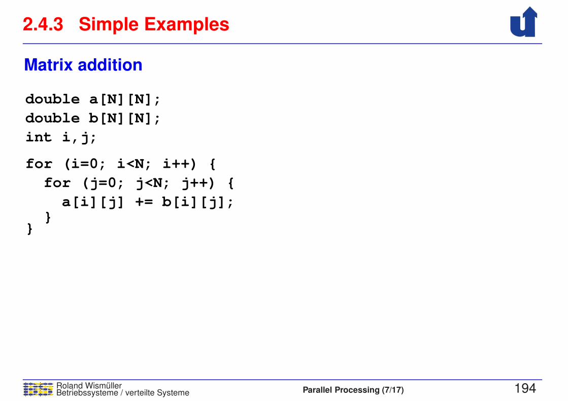
2.4.3 Simple Examples
Roland WismullerBetriebssysteme / verteilte Systeme Parallel Processing (7/17) 194
Matrix addition
double a[N][N];
double b[N][N];
int i,j;
for (i=0; i<N; i++) {
for (j=0; j<N; j++) {
a[i][j] += b[i][j]; }}

2.4.3 Simple Examples
Roland WismullerBetriebssysteme / verteilte Systeme Parallel Processing (7/17) 194
Matrix addition
double a[N][N];
double b[N][N];
int i,j;
for (i=0; i<N; i++) {
for (j=0; j<N; j++) {
a[i][j] += b[i][j]; }}
No dependences in ’j’ loop:
− ’b’ is read only
− Elements of ’a’ are always
read in the same ’j’ iteration,
in which thay are written
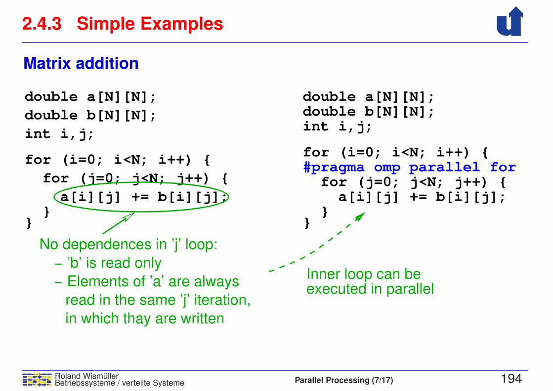
double a[N][N];
a[i][j] += b[i][j]; }}
double b[N][N];int i,j;
for (j=0; j<N; j++) {#pragma omp parallel forfor (i=0; i<N; i++) {
Inner loop can beexecuted in parallel
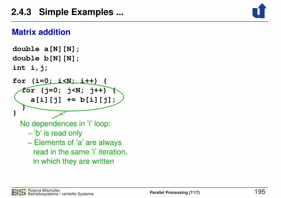
2.4.3 Simple Examples ...
Roland WismullerBetriebssysteme / verteilte Systeme Parallel Processing (7/17) 195
Matrix addition
double a[N][N];
double b[N][N];
int i,j;
for (i=0; i<N; i++) {
for (j=0; j<N; j++) {
a[i][j] += b[i][j]; }}
No dependences in ’i’ loop:
− ’b’ is read only
− Elements of ’a’ are always
in which they are written
read in the same ’i’ iteration,
a[i][j] += b[i][j]; }}
for (j=0; j<N; j++) {for (i=0; i<N; i++) {
double a[N][N];double b[N][N];int i,j;
#pragma omp parallel forprivate(j)
Outer loop can beexecuted in parallel
Advantage: less overhead!

Roland WismullerBetriebssysteme / verteilte Systeme Parallel Processing (8/17) ix
Roland Wismuller
Universitat Siegen
Tel.: 0271/740-4050, Buro: H-B 8404
Stand: January 23, 2018
Parallel Processing
WS 2017/18
13.11.2017
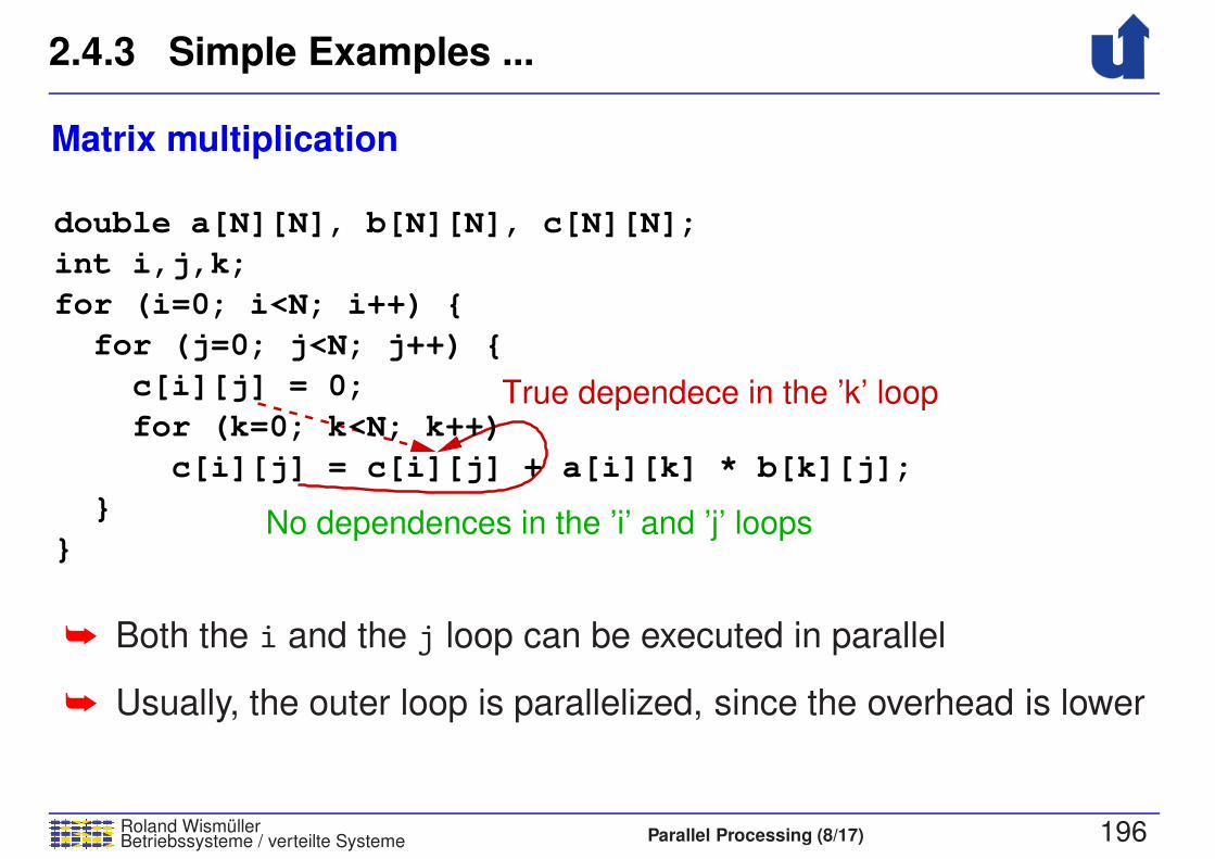
2.4.3 Simple Examples ...
Roland WismullerBetriebssysteme / verteilte Systeme Parallel Processing (8/17) 196
Matrix multiplication
No dependences in the ’i’ and ’j’ loops
True dependece in the ’k’ loop
double a[N][N], b[N][N], c[N][N];
int i,j,k;
for (j=0; j<N; j++) {
c[i][j] = 0;
for (k=0; k<N; k++)
c[i][j] = c[i][j] + a[i][k] * b[k][j];
}
for (i=0; i<N; i++) {
}
➥ Both the i and the j loop can be executed in parallel
➥ Usually, the outer loop is parallelized, since the overhead is lower

2.4.3 Simple Examples ...
Roland WismullerBetriebssysteme / verteilte Systeme Parallel Processing (8/17) 197
Removing dependences
double a[N], b[N];
int i;
a[i−1] = val;
}
a[i−1] = b[0];
b[i−1] = a[i] * a[i];
for (i=1; i<N; i++) {
double val = 1.2;
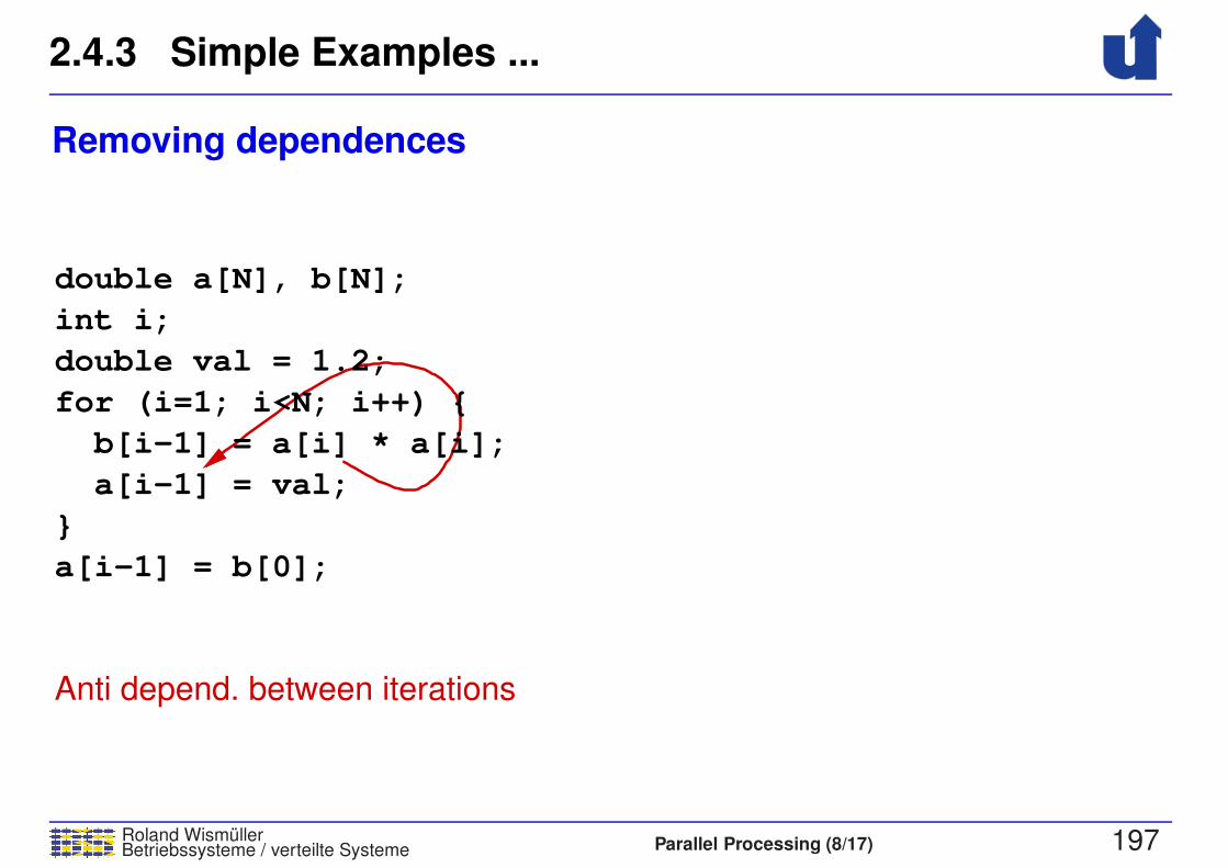
2.4.3 Simple Examples ...
Roland WismullerBetriebssysteme / verteilte Systeme Parallel Processing (8/17) 197
Removing dependences
Anti depend. between iterations
double a[N], b[N];
int i;
a[i−1] = val;
}
a[i−1] = b[0];
b[i−1] = a[i] * a[i];
for (i=1; i<N; i++) {
double val = 1.2;
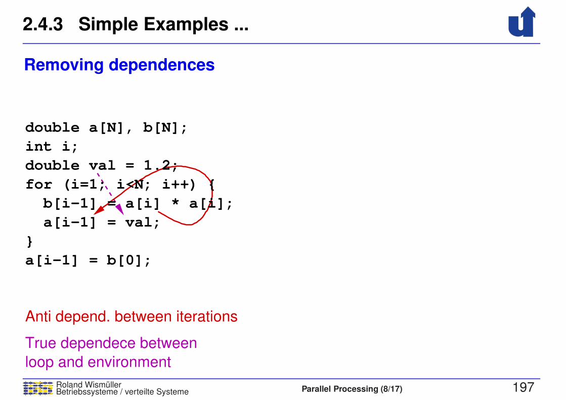
2.4.3 Simple Examples ...
Roland WismullerBetriebssysteme / verteilte Systeme Parallel Processing (8/17) 197
Removing dependences
True dependece between
loop and environment
Anti depend. between iterations
double a[N], b[N];
int i;
a[i−1] = val;
}
a[i−1] = b[0];
b[i−1] = a[i] * a[i];
for (i=1; i<N; i++) {
double val = 1.2;
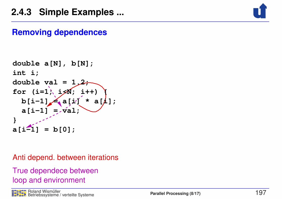
2.4.3 Simple Examples ...
Roland WismullerBetriebssysteme / verteilte Systeme Parallel Processing (8/17) 197
Removing dependences
True dependece between
loop and environment
Anti depend. between iterations
double a[N], b[N];
int i;
a[i−1] = val;
}
a[i−1] = b[0];
b[i−1] = a[i] * a[i];
for (i=1; i<N; i++) {
double val = 1.2;
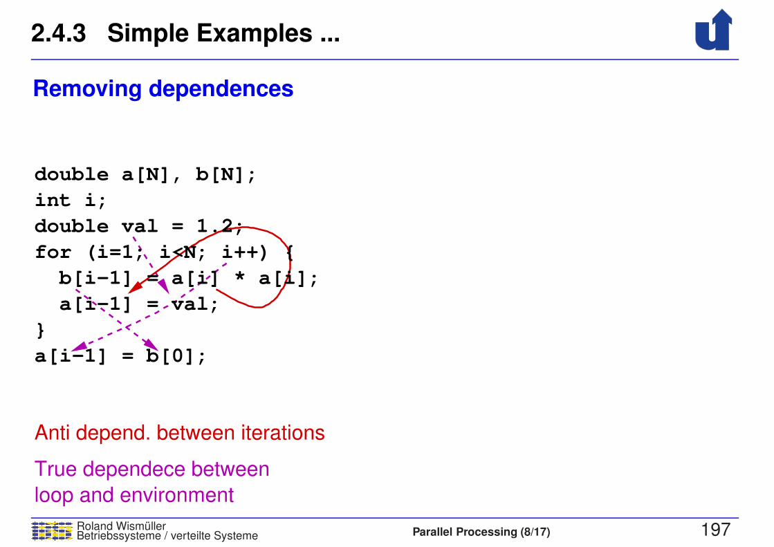
2.4.3 Simple Examples ...
Roland WismullerBetriebssysteme / verteilte Systeme Parallel Processing (8/17) 197
Removing dependences
True dependece between
loop and environment
Anti depend. between iterations
double a[N], b[N];
int i;
a[i−1] = val;
}
a[i−1] = b[0];
b[i−1] = a[i] * a[i];
for (i=1; i<N; i++) {
double val = 1.2;

2.4.3 Simple Examples ...
Roland WismullerBetriebssysteme / verteilte Systeme Parallel Processing (8/17) 197
Removing dependences
lastprivate(i) + barriers
Loop splitting + barrier
double a[N], b[N];int i;
{
b[i−1] = a[i] * a[i];
a[i−1] = val;for (i=1; i<N; i++)
#pragma omp for for (i=1; i<N; i++)
#pragma omp for lastprivate(i)
a[i−1] = b[0];}
double val = 1.2;#pragma omp parallel
True dependece between
loop and environment
Anti depend. between iterations
double a[N], b[N];
int i;
a[i−1] = val;
}
a[i−1] = b[0];
b[i−1] = a[i] * a[i];
for (i=1; i<N; i++) {
double val = 1.2;
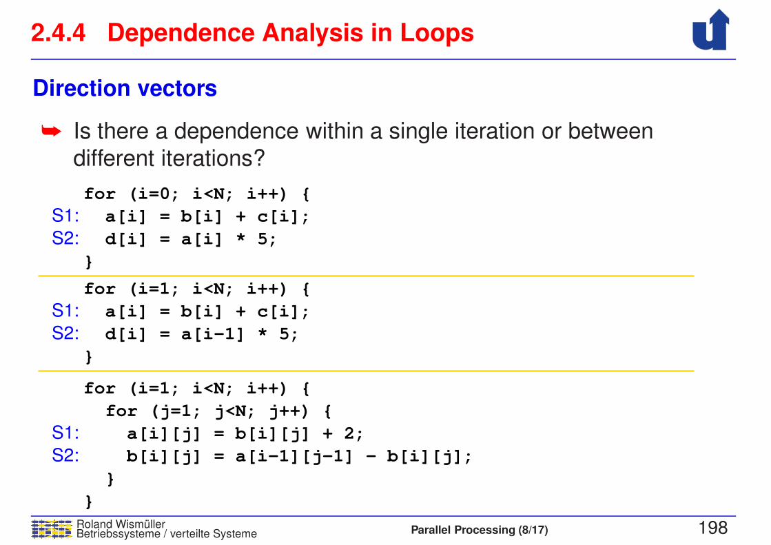
2.4.4 Dependence Analysis in Loops
Roland WismullerBetriebssysteme / verteilte Systeme Parallel Processing (8/17) 198
Direction vectors
➥ Is there a dependence within a single iteration or between
different iterations?
S1:
S2:
S2:
S1:
S1:
S2:
for (i=1; i<N; i++) {
a[i] = b[i] + c[i];
d[i] = a[i−1] * 5;
}
for (i=1; i<N; i++) {
}
for (i=0; i<N; i++) {
d[i] = a[i] * 5;
}
a[i] = b[i] + c[i];
for (j=1; j<N; j++) {
a[i][j] = b[i][j] + 2;
b[i][j] = a[i−1][j−1] − b[i][j];
}
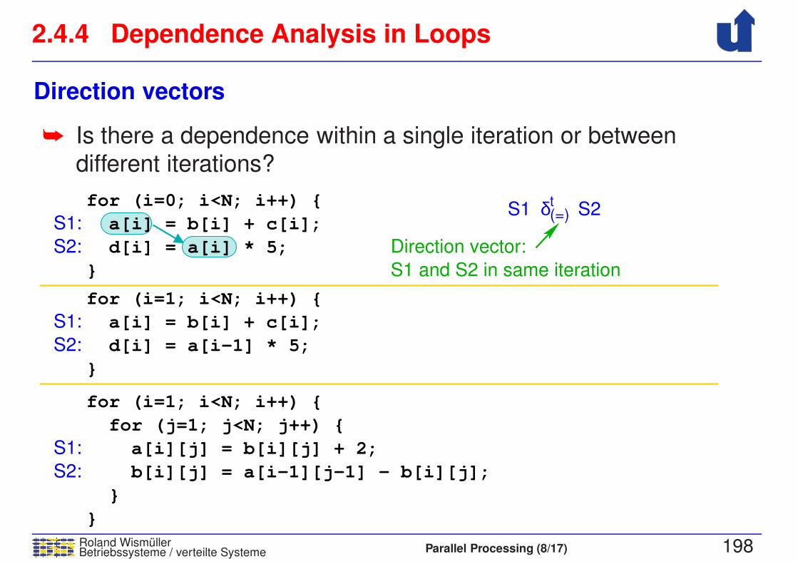
2.4.4 Dependence Analysis in Loops
Roland WismullerBetriebssysteme / verteilte Systeme Parallel Processing (8/17) 198
Direction vectors
➥ Is there a dependence within a single iteration or between
different iterations?
S1 and S2 in same iteration
Direction vector:
S1 δ(=) S2t
S1:
S2:
S2:
S1:
S1:
S2:
for (i=1; i<N; i++) {
a[i] = b[i] + c[i];
d[i] = a[i−1] * 5;
}
for (i=1; i<N; i++) {
}
for (i=0; i<N; i++) {
d[i] = a[i] * 5;
}
a[i] = b[i] + c[i];
for (j=1; j<N; j++) {
a[i][j] = b[i][j] + 2;
b[i][j] = a[i−1][j−1] − b[i][j];
}

2.4.4 Dependence Analysis in Loops
Roland WismullerBetriebssysteme / verteilte Systeme Parallel Processing (8/17) 198
Direction vectors
➥ Is there a dependence within a single iteration or between
different iterations?
Loop carried dependece
S1 in earlier iteration than S2
S1 δ(<) S2t
S1 and S2 in same iteration
Direction vector:
S1 δ(=) S2t
S1:
S2:
S2:
S1:
S1:
S2:
for (i=1; i<N; i++) {
a[i] = b[i] + c[i];
d[i] = a[i−1] * 5;
}
for (i=1; i<N; i++) {
}
for (i=0; i<N; i++) {
d[i] = a[i] * 5;
}
a[i] = b[i] + c[i];
for (j=1; j<N; j++) {
a[i][j] = b[i][j] + 2;
b[i][j] = a[i−1][j−1] − b[i][j];
}

2.4.4 Dependence Analysis in Loops
Roland WismullerBetriebssysteme / verteilte Systeme Parallel Processing (8/17) 198
Direction vectors
➥ Is there a dependence within a single iteration or between
different iterations?
S1 δ S2(=,=)a
Loop carried dependece
S1 in earlier iteration than S2
S1 δ(<) S2t
S1 and S2 in same iteration
Direction vector:
S1 δ(=) S2t
S1:
S2:
S2:
S1:
S1:
S2:
for (i=1; i<N; i++) {
a[i] = b[i] + c[i];
d[i] = a[i−1] * 5;
}
for (i=1; i<N; i++) {
}
for (i=0; i<N; i++) {
d[i] = a[i] * 5;
}
a[i] = b[i] + c[i];
for (j=1; j<N; j++) {
a[i][j] = b[i][j] + 2;
b[i][j] = a[i−1][j−1] − b[i][j];
}
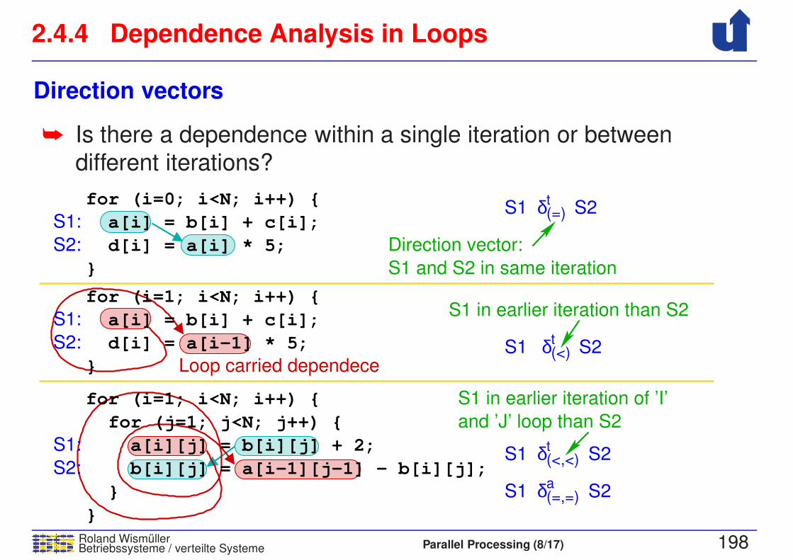
2.4.4 Dependence Analysis in Loops
Roland WismullerBetriebssysteme / verteilte Systeme Parallel Processing (8/17) 198
Direction vectors
➥ Is there a dependence within a single iteration or between
different iterations?
S1 δ S2(=,=)a
and ’J’ loop than S2
S1 in earlier iteration of ’I’
S1 δ(<,<) S2t
Loop carried dependece
S1 in earlier iteration than S2
S1 δ(<) S2t
S1 and S2 in same iteration
Direction vector:
S1 δ(=) S2t
S1:
S2:
S2:
S1:
S1:
S2:
for (i=1; i<N; i++) {
a[i] = b[i] + c[i];
d[i] = a[i−1] * 5;
}
for (i=1; i<N; i++) {
}
for (i=0; i<N; i++) {
d[i] = a[i] * 5;
}
a[i] = b[i] + c[i];
for (j=1; j<N; j++) {
a[i][j] = b[i][j] + 2;
b[i][j] = a[i−1][j−1] − b[i][j];
}
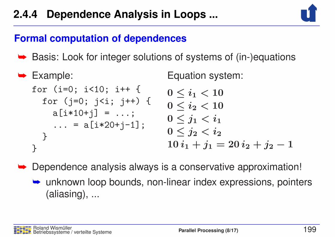
2.4.4 Dependence Analysis in Loops ...
Roland WismullerBetriebssysteme / verteilte Systeme Parallel Processing (8/17) 199
Formal computation of dependences
➥ Basis: Look for integer solutions of systems of (in-)equations
➥ Example:
for (i=0; i<10; i++ {
for (j=0; j<i; j++) {
a[i*10+j] = ...;
... = a[i*20+j-1];
}
}
Equation system:
0 ≤ i1 < 10
0 ≤ i2 < 10
0 ≤ j1 < i10 ≤ j2 < i210 i1 + j1 = 20 i2 + j2 − 1
➥ Dependence analysis always is a conservative approximation!
➥ unknown loop bounds, non-linear index expressions, pointers
(aliasing), ...
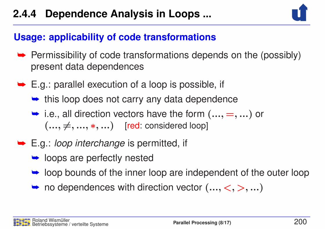
2.4.4 Dependence Analysis in Loops ...
Roland WismullerBetriebssysteme / verteilte Systeme Parallel Processing (8/17) 200
Usage: applicability of code transformations
➥ Permissibility of code transformations depends on the (possibly)
present data dependences
➥ E.g.: parallel execution of a loop is possible, if
➥ this loop does not carry any data dependence
➥ i.e., all direction vectors have the form (...,=, ...) or
(..., 6=, ..., ∗, ...) [red: considered loop]
➥ E.g.: loop interchange is permitted, if
➥ loops are perfectly nested
➥ loop bounds of the inner loop are independent of the outer loop
➥ no dependences with direction vector (..., <,>, ...)

2.4.4 Dependence Analysis in Loops ...
Roland WismullerBetriebssysteme / verteilte Systeme Parallel Processing (8/17) 201
Example: block algorithm for matrix multiplication
DO IT = 1,N,IS
DO JT = 1,N,JS
DO KT = 1,N,KS
DO I = IT, MIN(N,IT+IS−1)
DO J = JT, MIN(N,JT+JS−1)
DO K = KT, MIN(N,KT+KS−1)
A(I,J)=A(I,J)+B(I,K)*C(K,J)
DO I = 1,N
DO IT = 1,N,IS
DO JT = 1,N,JS
DO KT = 1,N,KS
A(I,J)=A(I,J)+B(I,K)*C(K,J)
DO J = 1,N
DO K = 1,N
A(I,J)=A(I,J)+B(I,K)*C(K,J)
Strip
mining DO IT = 1,N,IS
DO I = 1,N
DO I = IT, MIN(N,IT+IS−1)
DO I = IT, MIN(N,IT+IS−1)
DO J = JT, MIN(N,JT+JS−1)
DO K = KT, MIN(N,KT+KS−1)
Loop
interchange
2.5 Example: The Jacobi and Gauss/Seidel Methods
Roland WismullerBetriebssysteme / verteilte Systeme Parallel Processing (8/17) 202
Numerical solution of the equations for thermal conduction
➥ Concrete problem: thin metal plate
➥ given: temperature profile of the boundary
➥ gesucht: temperature profile of the interior
➥ Approach:
➥ discretization: consider the temperature only at equidistant
grid points
➥ 2D array of temperature values
➥ iterative solution: compute ever more exact approximations
➥ new approximations for the temperature of a grid point:
mean value of the temperatures of the neighboring points
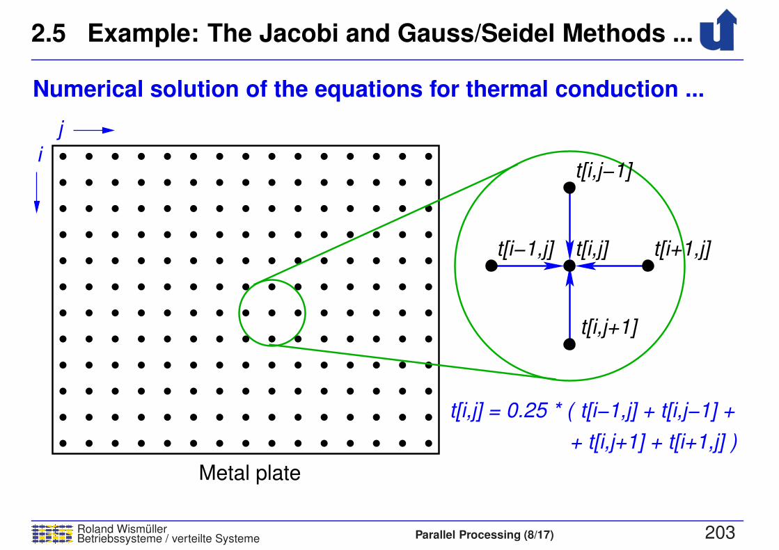
2.5 Example: The Jacobi and Gauss/Seidel Methods ...
Roland WismullerBetriebssysteme / verteilte Systeme Parallel Processing (8/17) 203
Numerical solution of the equations for thermal conduction ...
j
i
t[i,j] = 0.25 * ( t[i−1,j] + t[i,j−1] +
+ t[i,j+1] + t[i+1,j] )
Metal plate
t[i,j]t[i−1,j] t[i+1,j]
t[i,j−1]
t[i,j+1]

2.5 Example: The Jacobi and Gauss/Seidel Methods ...
Roland WismullerBetriebssysteme / verteilte Systeme Parallel Processing (8/17) 204
Variants of the method
➥ Jacobi iteration
➥ to compute the new values, only the values of the last iteration
are used
➥ computation uses two matrices
➥ Gauss/Seidel relaxation
➥ to compute the new values, also some values of the current
iteration are used:
➥ t[i− 1, j] and t[i, j − 1]
➥ computation uses only one matrix
➥ usually faster convergence as compared to Jacobi
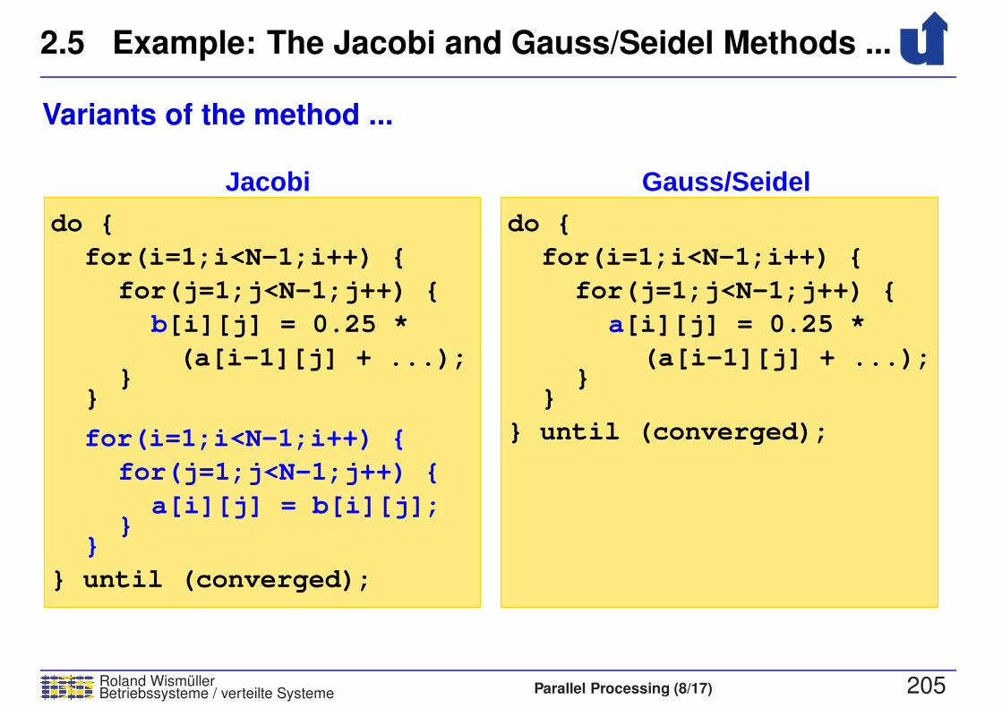
2.5 Example: The Jacobi and Gauss/Seidel Methods ...
Roland WismullerBetriebssysteme / verteilte Systeme Parallel Processing (8/17) 205
Variants of the method ...
Jacobi Gauss/Seidel
for(i=1;i<N−1;i++) {
for(j=1;j<N−1;j++) {
}}
(a[i−1][j] + ...);
do {
} until (converged);
do {
for(i=1;i<N−1;i++) {
for(j=1;j<N−1;j++) {
(a[i−1][j] + ...);}
}
} until (converged);
b a[i][j] = 0.25 * [i][j] = 0.25 *
a[i][j] = b[i][j];}
}
for(j=1;j<N−1;j++) {
for(i=1;i<N−1;i++) {
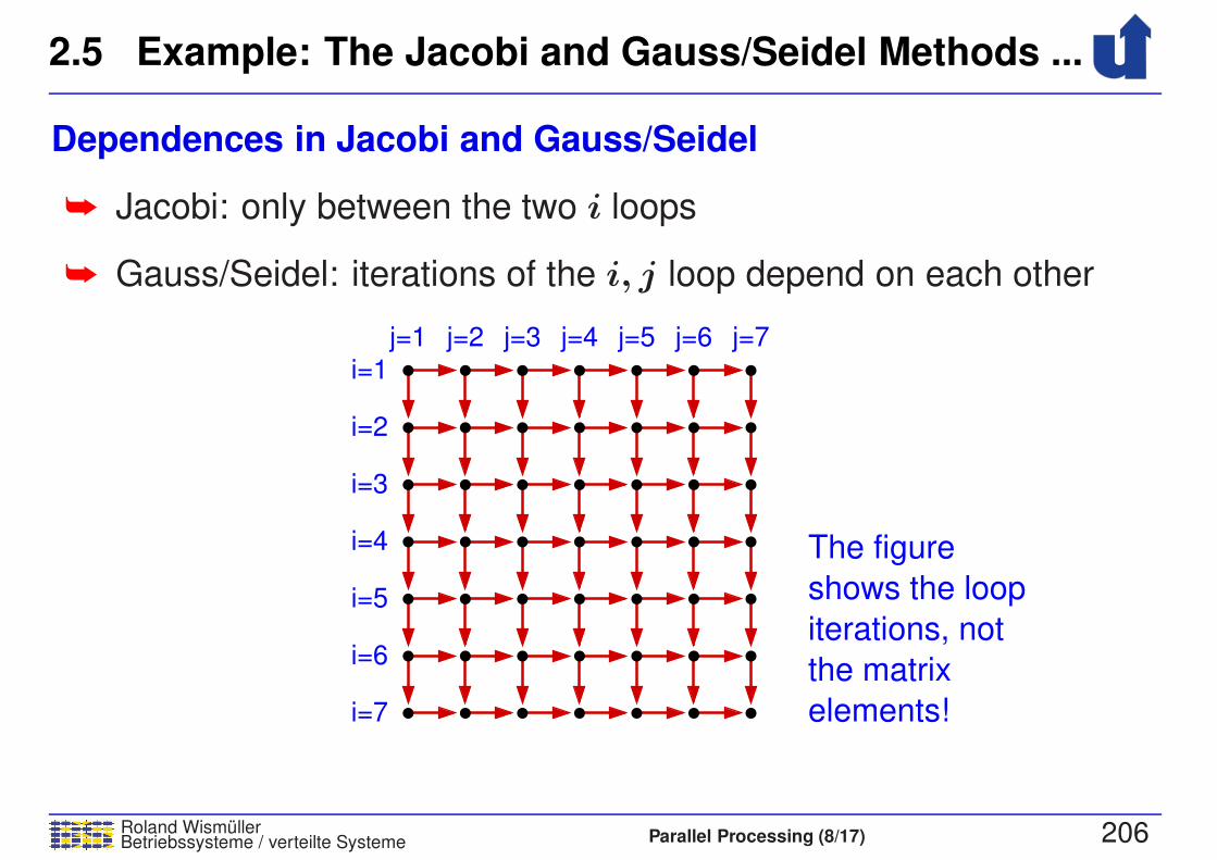
2.5 Example: The Jacobi and Gauss/Seidel Methods ...
Roland WismullerBetriebssysteme / verteilte Systeme Parallel Processing (8/17) 206
Dependences in Jacobi and Gauss/Seidel
➥ Jacobi: only between the two i loops
➥ Gauss/Seidel: iterations of the i, j loop depend on each other
i=1
i=2
i=3
i=4
i=5
i=6
i=7
j=1 j=2 j=3 j=4 j=5 j=6 j=7
The figure
elements!
the matrix
iterations, not
shows the loop
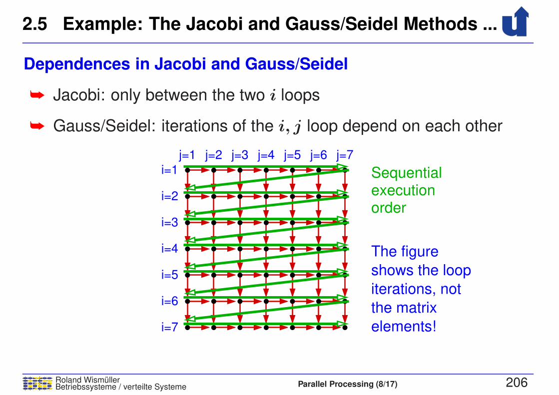
Sequentialexecutionorder
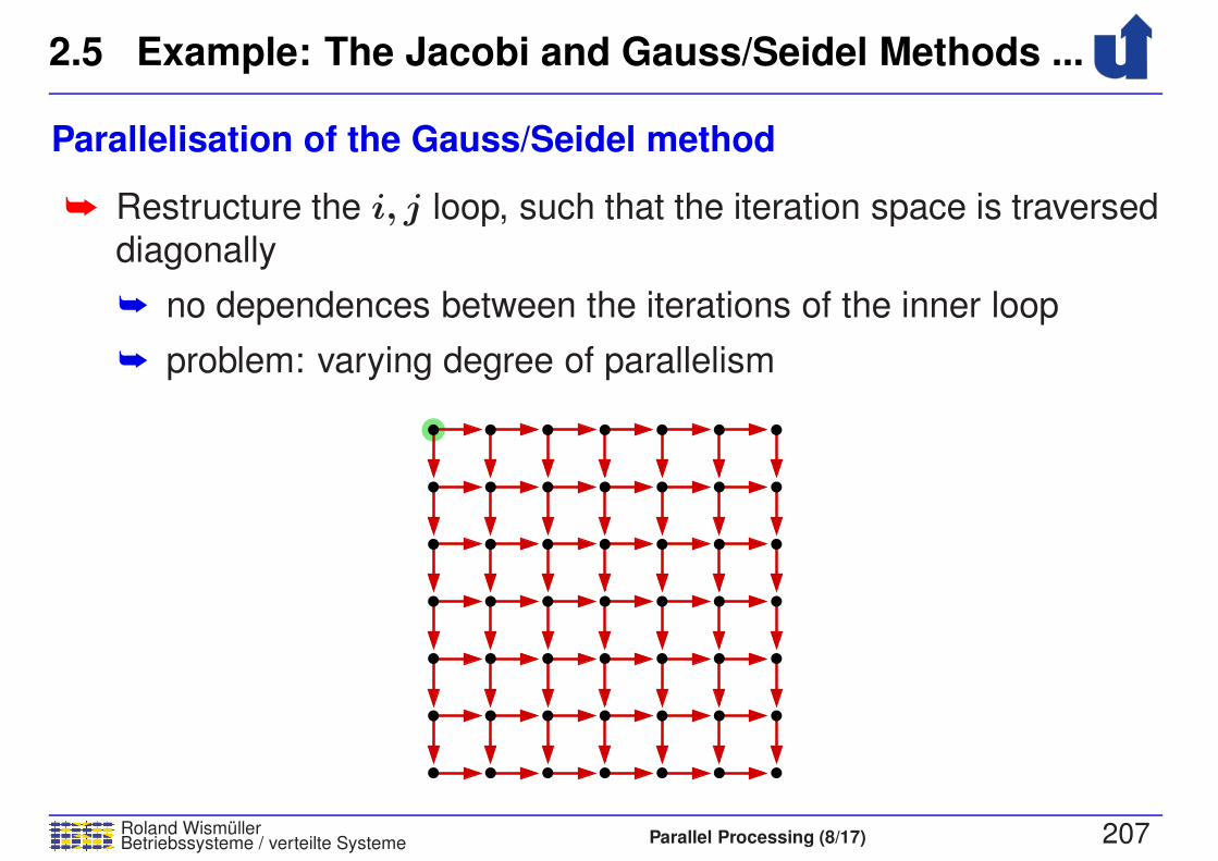
2.5 Example: The Jacobi and Gauss/Seidel Methods ...
Roland WismullerBetriebssysteme / verteilte Systeme Parallel Processing (8/17) 207
Parallelisation of the Gauss/Seidel method
➥ Restructure the i, j loop, such that the iteration space is traversed
diagonally
➥ no dependences between the iterations of the inner loop
➥ problem: varying degree of parallelism
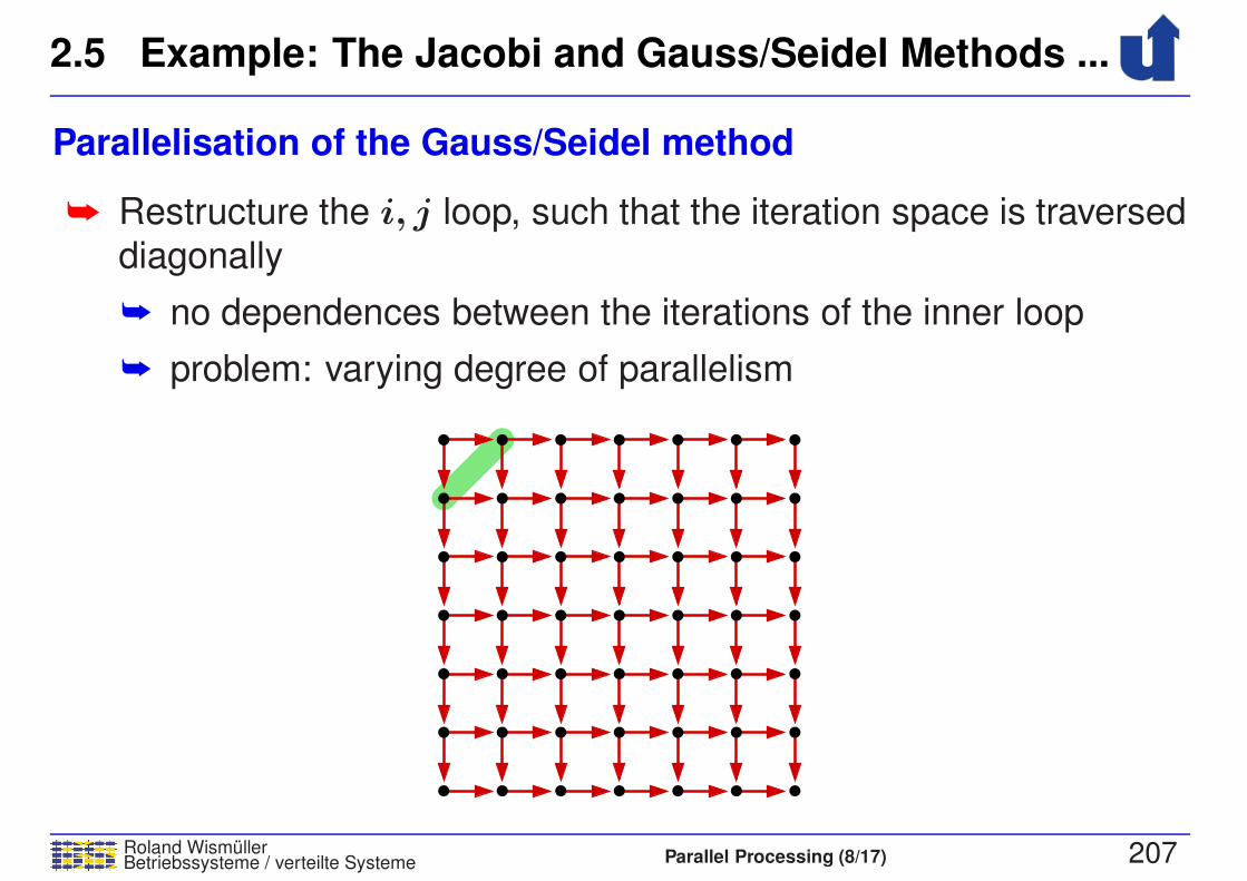
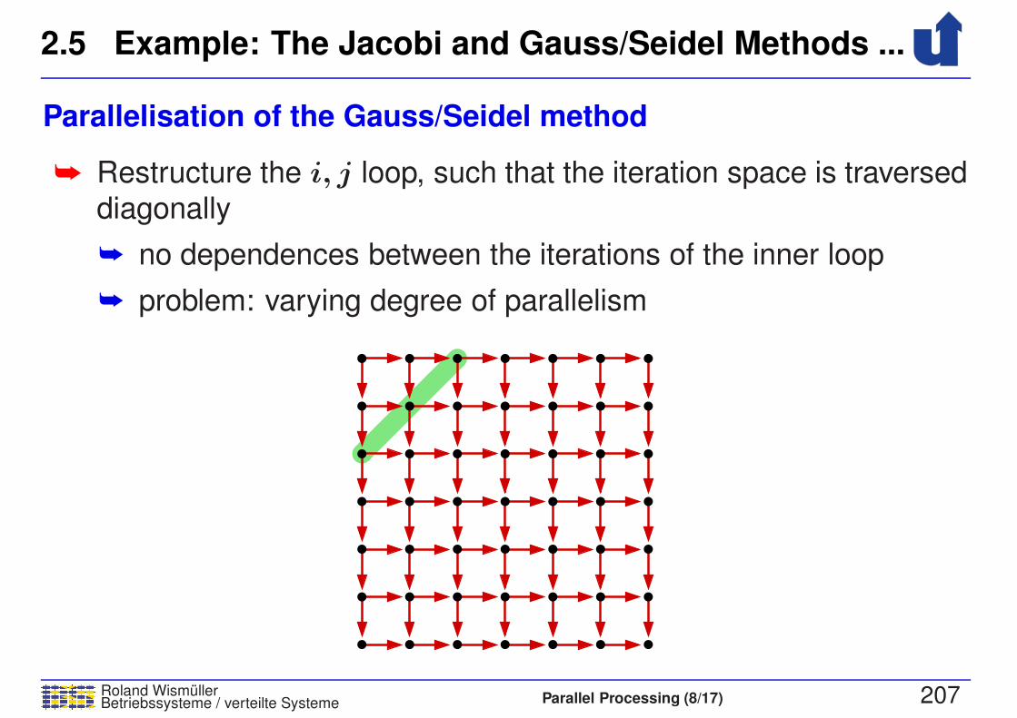
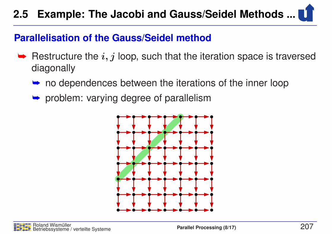
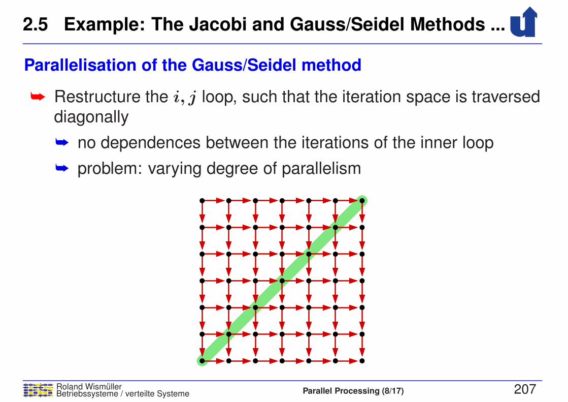
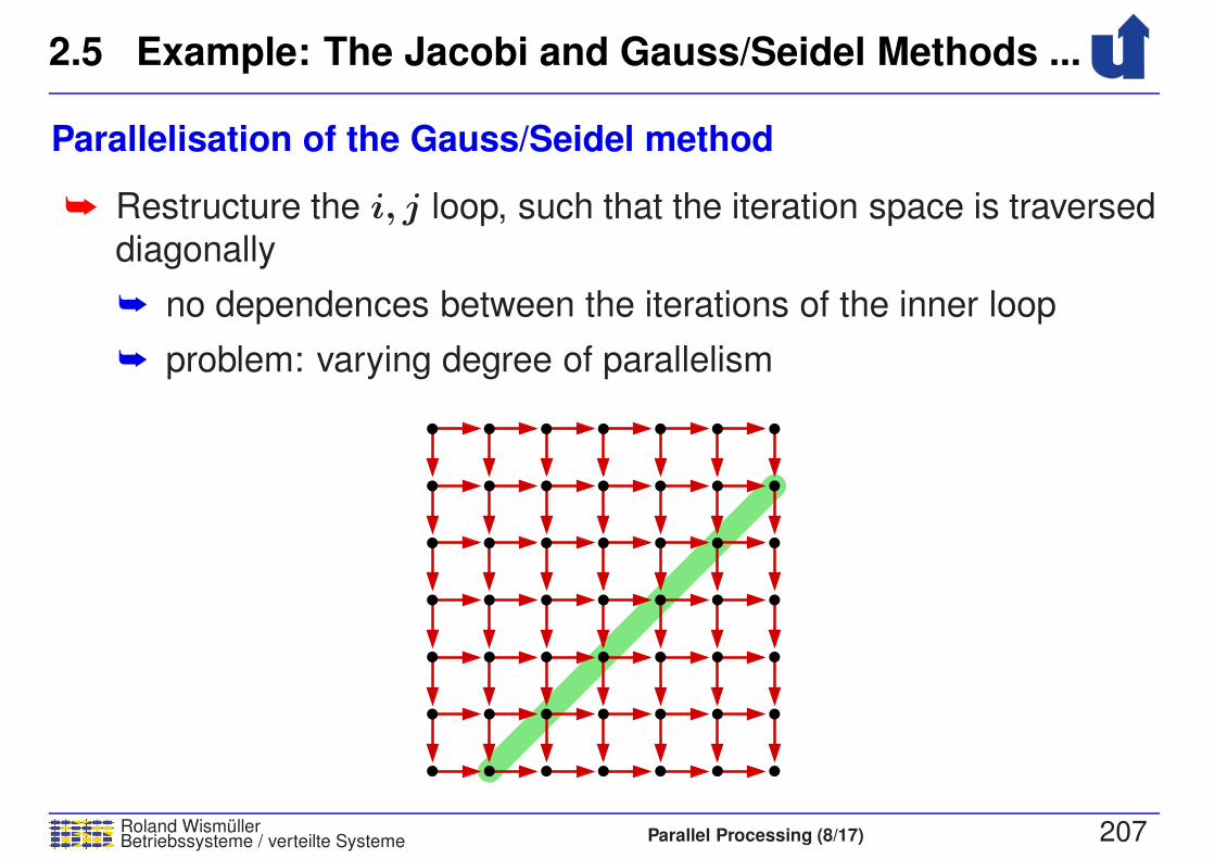
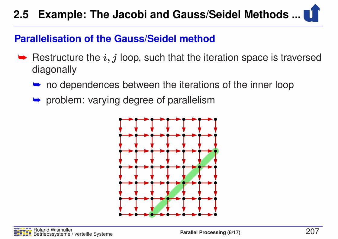
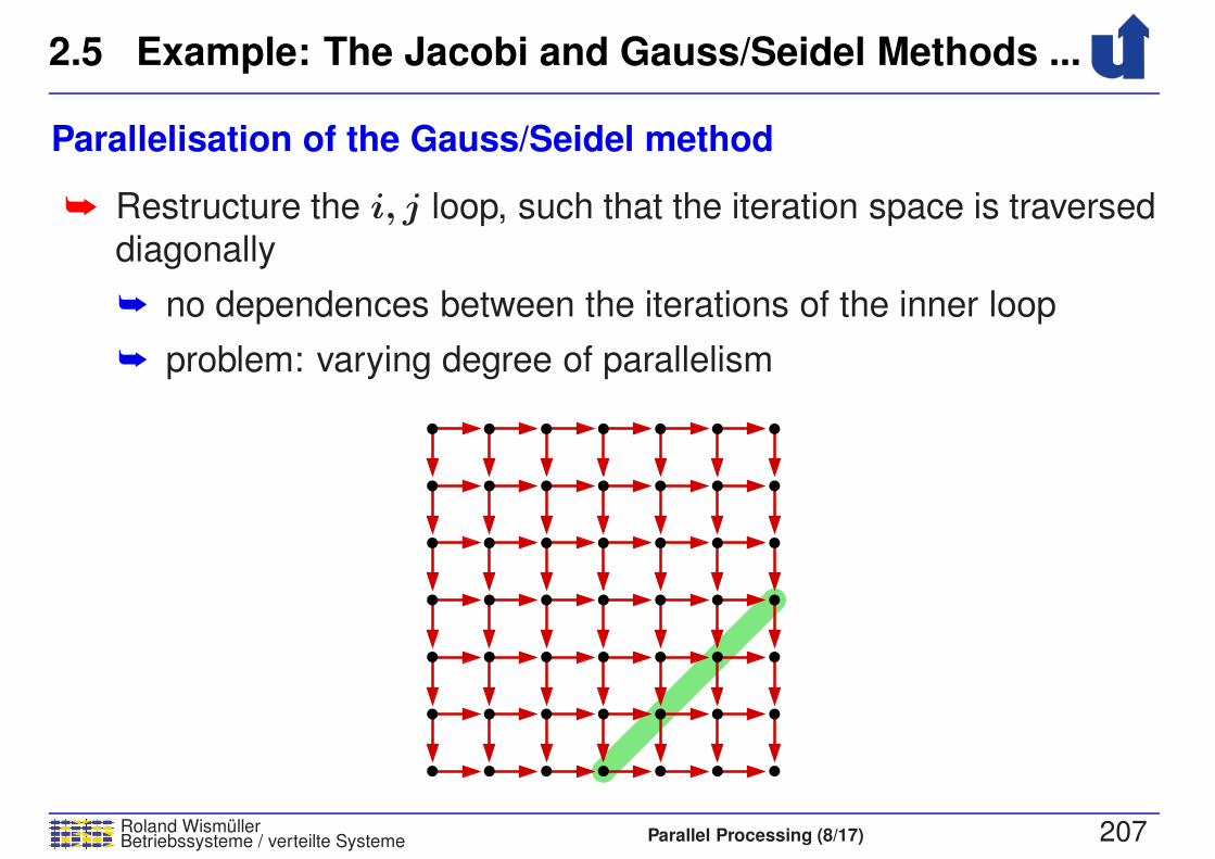
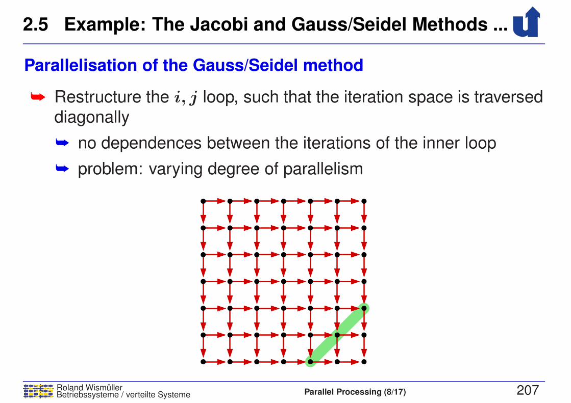
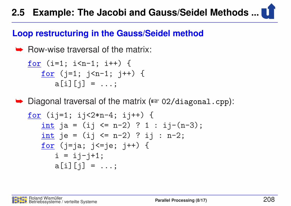
2.5 Example: The Jacobi and Gauss/Seidel Methods ...
Roland WismullerBetriebssysteme / verteilte Systeme Parallel Processing (8/17) 208
Loop restructuring in the Gauss/Seidel method
➥ Row-wise traversal of the matrix:
for (i=1; i<n-1; i++) {
for (j=1; j<n-1; j++) {
a[i][j] = ...;
➥ Diagonal traversal of the matrix (☞ 02/diagonal.cpp):
for (ij=1; ij<2*n-4; ij++) {
int ja = (ij <= n-2) ? 1 : ij-(n-3);
int je = (ij <= n-2) ? ij : n-2;
for (j=ja; j<=je; j++) {
i = ij-j+1;
a[i][j] = ...;
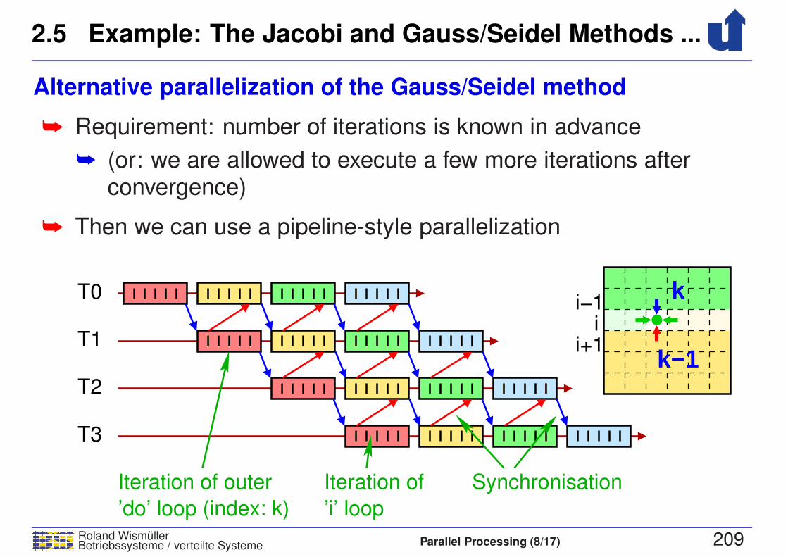
2.5 Example: The Jacobi and Gauss/Seidel Methods ...
Roland WismullerBetriebssysteme / verteilte Systeme Parallel Processing (8/17) 209
Alternative parallelization of the Gauss/Seidel method
➥ Requirement: number of iterations is known in advance
➥ (or: we are allowed to execute a few more iterations afterconvergence)
➥ Then we can use a pipeline-style parallelization
i+1i
i−1T0
T1
T2
T3
k
k−1
Iteration of
’i’ loop
SynchronisationIteration of outer
’do’ loop (index: k)
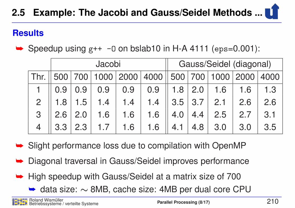
2.5 Example: The Jacobi and Gauss/Seidel Methods ...
Roland WismullerBetriebssysteme / verteilte Systeme Parallel Processing (8/17) 210
Results
➥ Speedup using g++ -O on bslab10 in H-A 4111 (eps=0.001):
Jacobi Gauss/Seidel (diagonal)
Thr. 500 700 1000 2000 4000 500 700 1000 2000 4000
1 0.9 0.9 0.9 0.9 0.9 1.8 2.0 1.6 1.6 1.3
2 1.8 1.5 1.4 1.4 1.4 3.5 3.7 2.1 2.6 2.6
3 2.6 2.0 1.6 1.6 1.6 4.0 4.4 2.5 2.7 3.1
4 3.3 2.3 1.7 1.6 1.6 4.1 4.8 3.0 3.0 3.5
➥ Slight performance loss due to compilation with OpenMP
➥ Diagonal traversal in Gauss/Seidel improves performance
➥ High speedup with Gauss/Seidel at a matrix size of 700
➥ data size: ∼ 8MB, cache size: 4MB per dual core CPU

2.5 Example: The Jacobi and Gauss/Seidel Methods ...
Roland WismullerBetriebssysteme / verteilte Systeme Parallel Processing (8/17) 211
Speedup on the HorUS cluster: Jacobi
Threads
Sp
ee
du
p
0
2
4
6
8
10
2 4 6 8 10 12
4000
2000
700
500
1000
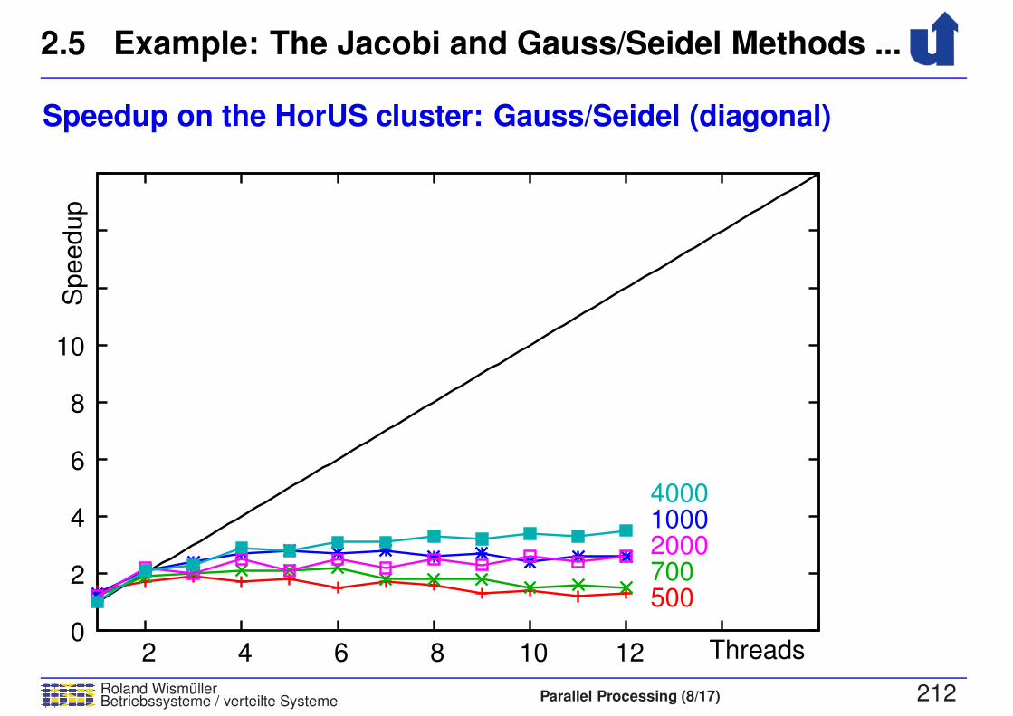
2.5 Example: The Jacobi and Gauss/Seidel Methods ...
Roland WismullerBetriebssysteme / verteilte Systeme Parallel Processing (8/17) 212
Speedup on the HorUS cluster: Gauss/Seidel (diagonal)
Threads
Sp
ee
du
p
0
2
4
6
8
10
2 4 6 8 10 12
700500
200010004000

2.5 Example: The Jacobi and Gauss/Seidel Methods ...
Roland WismullerBetriebssysteme / verteilte Systeme Parallel Processing (8/17) 213
Speedup on the HorUS cluster: Gauss/Seidel (pipeline)
Threads
Sp
ee
du
p
0
2
4
6
8
10
2 4 6 8 10 12
500700
200040001000
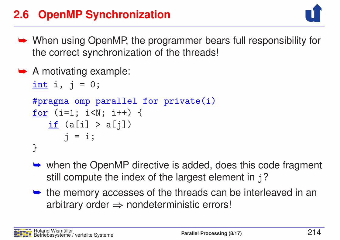
2.6 OpenMP Synchronization
Roland WismullerBetriebssysteme / verteilte Systeme Parallel Processing (8/17) 214
➥ When using OpenMP, the programmer bears full responsibility for
the correct synchronization of the threads!
➥ A motivating example:
int i, j = 0;
#pragma omp parallel for private(i)
for (i=1; i<N; i++) {
if (a[i] > a[j])
j = i;
}
➥ when the OpenMP directive is added, does this code fragment
still compute the index of the largest element in j?
➥ the memory accesses of the threads can be interleaved in an
arbitrary order⇒ nondeterministic errors!
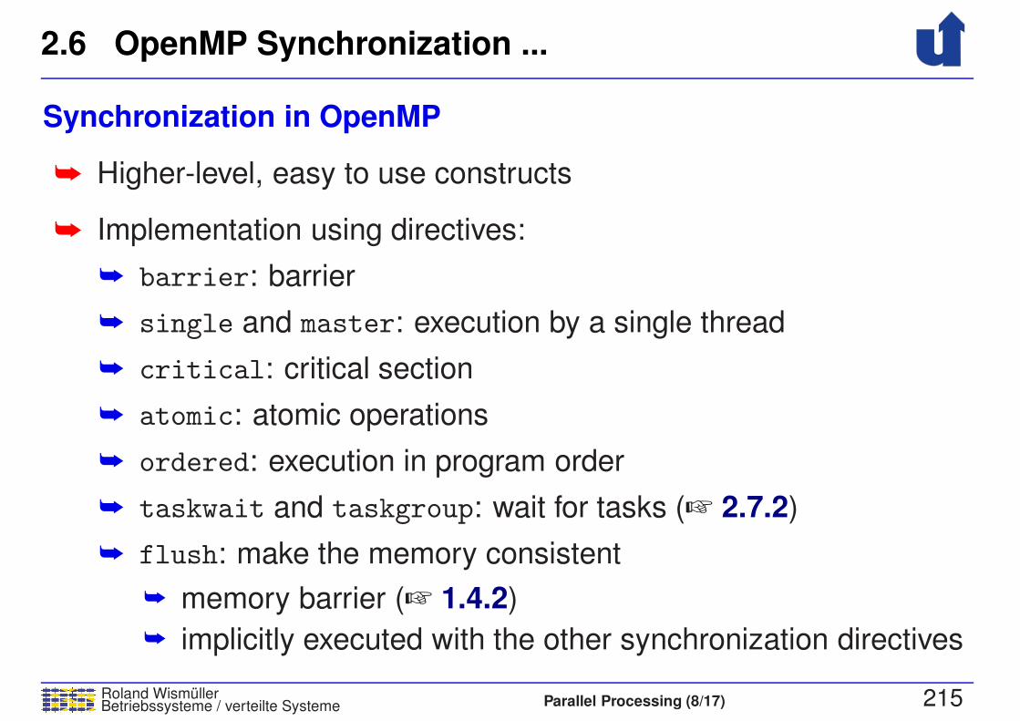
2.6 OpenMP Synchronization ...
Roland WismullerBetriebssysteme / verteilte Systeme Parallel Processing (8/17) 215
Synchronization in OpenMP
➥ Higher-level, easy to use constructs
➥ Implementation using directives:
➥ barrier: barrier
➥ single and master: execution by a single thread
➥ critical: critical section
➥ atomic: atomic operations
➥ ordered: execution in program order
➥ taskwait and taskgroup: wait for tasks (☞ 2.7.2)
➥ flush: make the memory consistent
➥ memory barrier (☞ 1.4.2)
➥ implicitly executed with the other synchronization directives

Roland WismullerBetriebssysteme / verteilte Systeme Parallel Processing (9/17) x
Roland Wismuller
Universitat Siegen
Tel.: 0271/740-4050, Buro: H-B 8404
Stand: January 23, 2018
Parallel Processing
WS 2017/18
27.11.2017

2.6 OpenMP Synchronization ...
Roland WismullerBetriebssysteme / verteilte Systeme Parallel Processing (9/17) 216
Barrier
#pragma omp barrier
➥ Synchronizes all threads
➥ each thread waits, until all other threads have reached the
barrier
➥ Implicit barrier at the end of for, sections, and single directives
➥ can be removed by specifying the option nowait
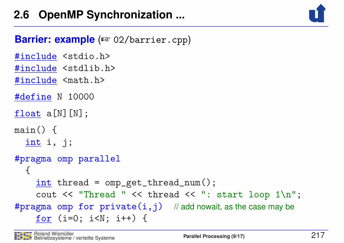
2.6 OpenMP Synchronization ...
Roland WismullerBetriebssysteme / verteilte Systeme Parallel Processing (9/17) 217
Barrier: example (☞ 02/barrier.cpp)
#include <stdio.h>
#include <stdlib.h>
#include <math.h>
#define N 10000
float a[N][N];
main() {
int i, j;
#pragma omp parallel
{
int thread = omp_get_thread_num();
cout << "Thread " << thread << ": start loop 1\n";
#pragma omp for private(i,j) // add nowait, as the case may be
for (i=0; i<N; i++) {
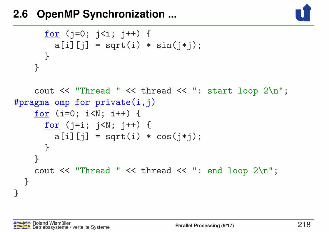
2.6 OpenMP Synchronization ...
Roland WismullerBetriebssysteme / verteilte Systeme Parallel Processing (9/17) 218
for (j=0; j<i; j++) {
a[i][j] = sqrt(i) * sin(j*j);
}
}
cout << "Thread " << thread << ": start loop 2\n";
#pragma omp for private(i,j)
for (i=0; i<N; i++) {
for (j=i; j<N; j++) {
a[i][j] = sqrt(i) * cos(j*j);
}
}
cout << "Thread " << thread << ": end loop 2\n";
}
}
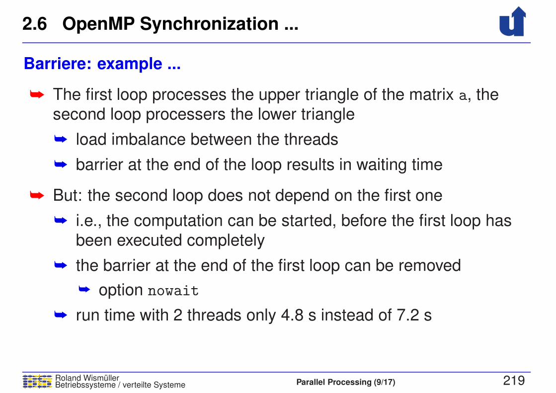
2.6 OpenMP Synchronization ...
Roland WismullerBetriebssysteme / verteilte Systeme Parallel Processing (9/17) 219
Barriere: example ...
➥ The first loop processes the upper triangle of the matrix a, the
second loop processers the lower triangle
➥ load imbalance between the threads
➥ barrier at the end of the loop results in waiting time
➥ But: the second loop does not depend on the first one
➥ i.e., the computation can be started, before the first loop has
been executed completely
➥ the barrier at the end of the first loop can be removed
➥ option nowait
➥ run time with 2 threads only 4.8 s instead of 7.2 s
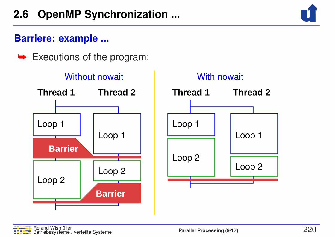
2.6 OpenMP Synchronization ...
Roland WismullerBetriebssysteme / verteilte Systeme Parallel Processing (9/17) 220
Barriere: example ...
➥ Executions of the program:
Loop 1
Loop 1
Loop 2Loop 2
Loop 1
Loop 1
Loop 2Loop 2
Without nowait With nowait
Thread 2Thread 1Thread 2Thread 1
Barrier
Barrier
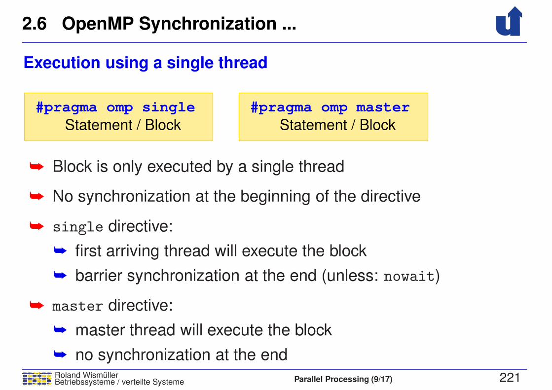
2.6 OpenMP Synchronization ...
Roland WismullerBetriebssysteme / verteilte Systeme Parallel Processing (9/17) 221
Execution using a single thread
#pragma omp single #pragma omp master
Statement / Block Statement / Block
➥ Block is only executed by a single thread
➥ No synchronization at the beginning of the directive
➥ single directive:
➥ first arriving thread will execute the block
➥ barrier synchronization at the end (unless: nowait)
➥ master directive:
➥ master thread will execute the block
➥ no synchronization at the end
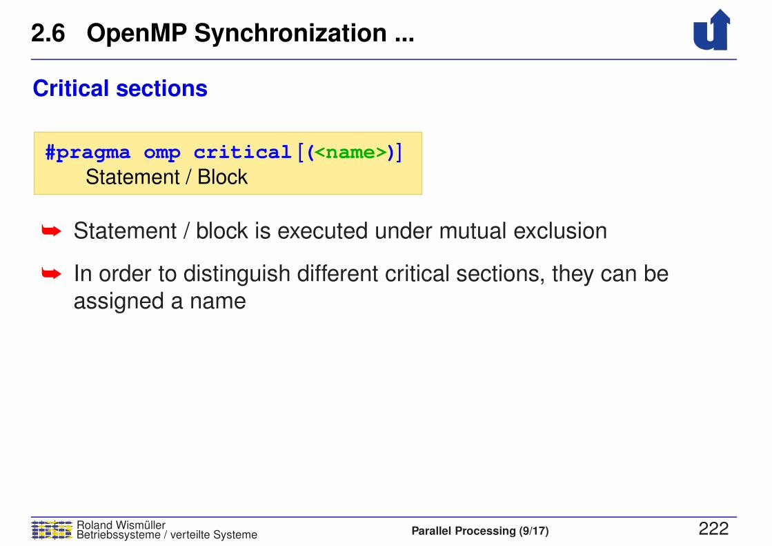
2.6 OpenMP Synchronization ...
Roland WismullerBetriebssysteme / verteilte Systeme Parallel Processing (9/17) 222
Critical sections
Statement / Block
#pragma omp critical [(<name>)]
➥ Statement / block is executed under mutual exclusion
➥ In order to distinguish different critical sections, they can be
assigned a name

2.6 OpenMP Synchronization ...
Roland WismullerBetriebssysteme / verteilte Systeme Parallel Processing (9/17) 223
Atomic operations
Statement / Block
#pragma omp atomic [ read write update capture] [seq_cst]|||
➥ Statement or block (only with capture) will be executed atomically
➥ usually by compiling it into special machine instrcutions
➥ Considerably more efficient than critical section
➥ The option defines the type of the atomic operation:
➥ read / write: atomic read / write
➥ update (default): atomic update of a variable
➥ capture: atomic update of a variable, while storing the old orthe new value, respectively
➥ Option seq cst: enforce memory consistency (flush)
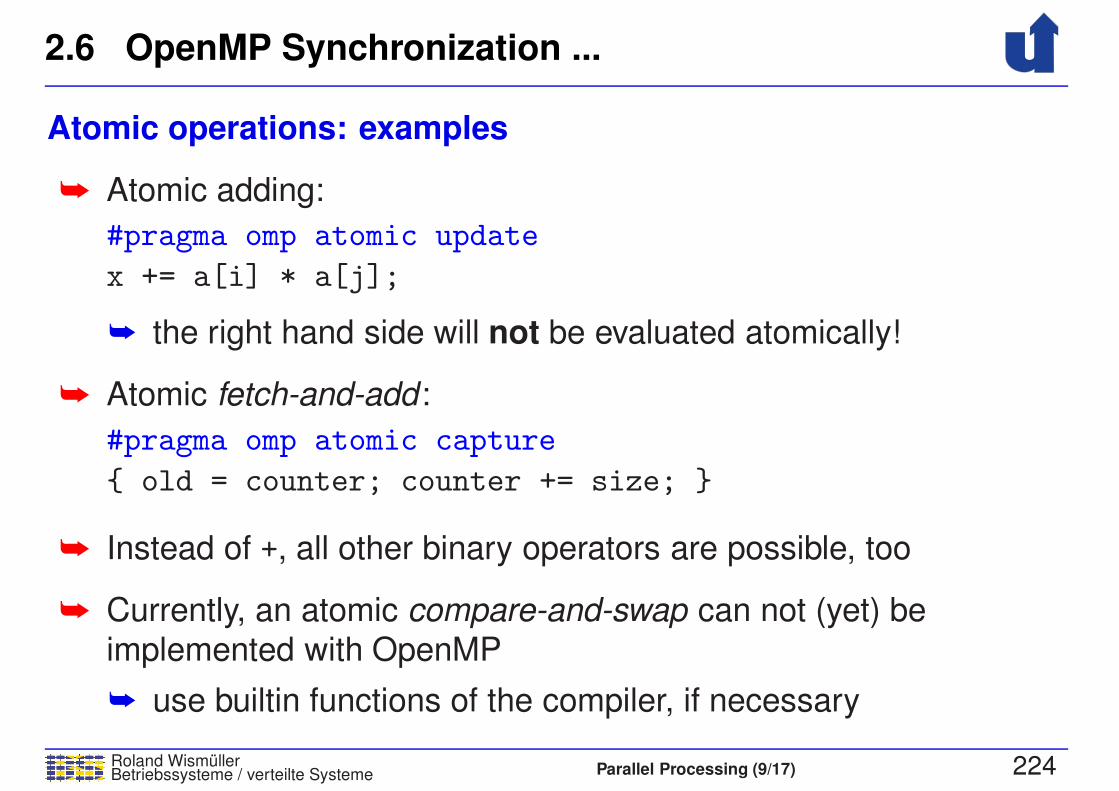
2.6 OpenMP Synchronization ...
Roland WismullerBetriebssysteme / verteilte Systeme Parallel Processing (9/17) 224
Atomic operations: examples
➥ Atomic adding:
#pragma omp atomic update
x += a[i] * a[j];
➥ the right hand side will not be evaluated atomically!
➥ Atomic fetch-and-add :
#pragma omp atomic capture
{ old = counter; counter += size; }
➥ Instead of +, all other binary operators are possible, too
➥ Currently, an atomic compare-and-swap can not (yet) be
implemented with OpenMP
➥ use builtin functions of the compiler, if necessary
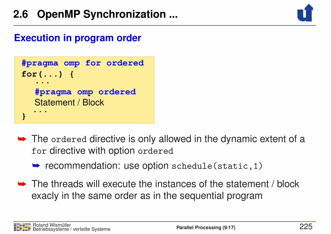
2.6 OpenMP Synchronization ...
Roland WismullerBetriebssysteme / verteilte Systeme Parallel Processing (9/17) 225
Execution in program order
#pragma omp for ordered
for(...) {...
Statement / Block...
}
#pragma omp ordered
➥ The ordered directive is only allowed in the dynamic extent of a
for directive with option ordered
➥ recommendation: use option schedule(static,1)
➥ The threads will execute the instances of the statement / block
exacly in the same order as in the sequential program

2.6 OpenMP Synchronization ...
Roland WismullerBetriebssysteme / verteilte Systeme Parallel Processing (9/17) 226
Execution with ordered
Barrier
Tim
e
Iterations
...
...
S2
S2
S2
i=0 i=2i=1 i=N−1
S2
#pragma omp for ordered
#pragma omp orderedS1;
S3;}
for(i=0; i<N; i++) {
S2;S1
S1S1 S1
S3
S3S3 S3

2.6 OpenMP Synchronization ...
Roland WismullerBetriebssysteme / verteilte Systeme Parallel Processing (9/17) 227
Reduction operations
➥ Often loops aggregate values, e.g.:
int a[N];
printf("sum=%d\n",sum);
sum += a[i];}
#pragma omp parallel for reduction(+: sum)
for (i=0; i<N; i++){
int i, sum = 0;
contains the sum of all elementsAt the end of the loop, ’sum’
➥ reduction saves us a critical section
➥ each thread first computes its partial sum in a private variable
➥ after the loop ends, the total sum is computed
➥ Instead of + is is also possible to use other operators:- * & | ^ && || min max
➥ in addition, user defined operators are possible
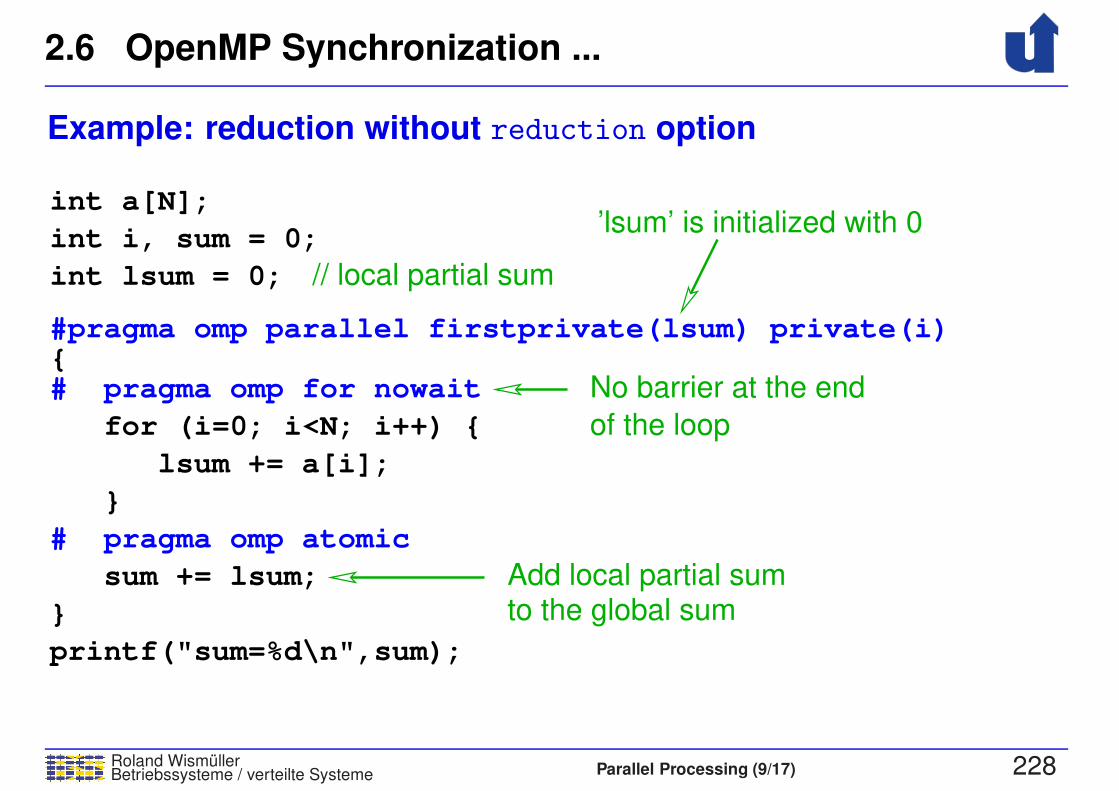
2.6 OpenMP Synchronization ...
Roland WismullerBetriebssysteme / verteilte Systeme Parallel Processing (9/17) 228
Example: reduction without reduction option
#pragma omp parallel firstprivate(lsum) private(i){
int lsum = 0; // local partial sum
’lsum’ is initialized with 0int a[N];
int i, sum = 0;
# pragma omp for nowait
for (i=0; i<N; i++) {
lsum += a[i];
}
# pragma omp atomic
sum += lsum;
No barrier at the end
of the loop
Add local partial sumto the global sum
printf("sum=%d\n",sum);
}
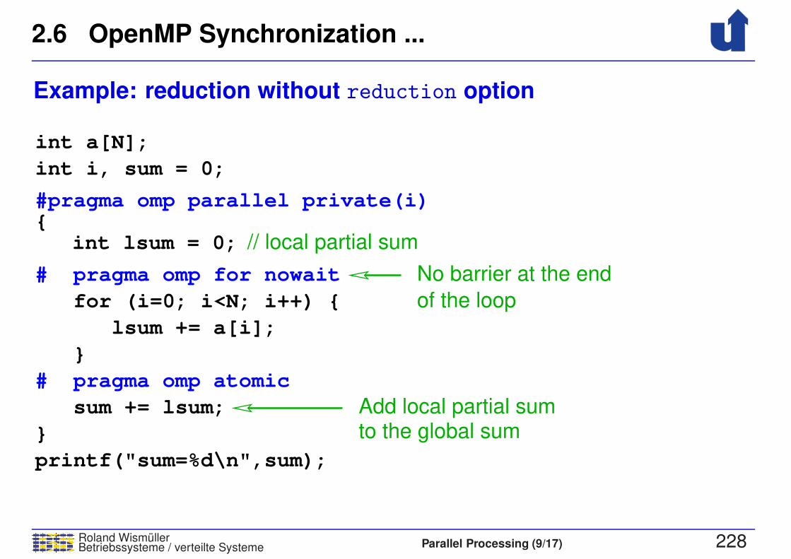
2.6 OpenMP Synchronization ...
Roland WismullerBetriebssysteme / verteilte Systeme Parallel Processing (9/17) 228
Example: reduction without reduction option
{#pragma omp parallel private(i)
int lsum = 0; // local partial sum
int a[N];
int i, sum = 0;
# pragma omp for nowait
for (i=0; i<N; i++) {
lsum += a[i];
}
# pragma omp atomic
sum += lsum;
No barrier at the end
of the loop
Add local partial sumto the global sum
printf("sum=%d\n",sum);
}
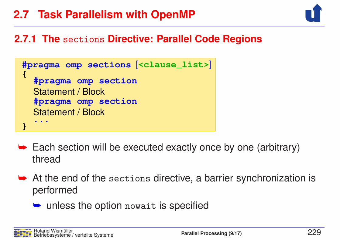
2.7 Task Parallelism with OpenMP
Roland WismullerBetriebssysteme / verteilte Systeme Parallel Processing (9/17) 229
2.7.1 The sections Directive: Parallel Code Regions
<clause_list>][{
#pragma omp section
}...Statement / Block
#pragma omp sectionStatement / Block
#pragma omp sections
➥ Each section will be executed exactly once by one (arbitrary)thread
➥ At the end of the sections directive, a barrier synchronization is
performed
➥ unless the option nowait is specified
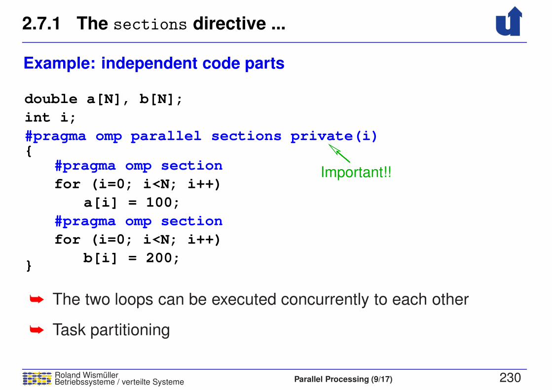
2.7.1 The sections directive ...
Roland WismullerBetriebssysteme / verteilte Systeme Parallel Processing (9/17) 230
Example: independent code parts
double a[N], b[N];
int i;
#pragma omp parallel sections private(i)
#pragma omp section
a[i] = 100;
#pragma omp section
b[i] = 200;}
Important!!
{
for (i=0; i<N; i++)
for (i=0; i<N; i++)
➥ The two loops can be executed concurrently to each other
➥ Task partitioning
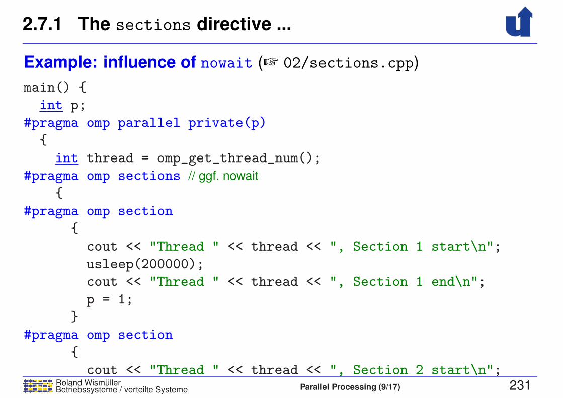
2.7.1 The sections directive ...
Roland WismullerBetriebssysteme / verteilte Systeme Parallel Processing (9/17) 231
Example: influence of nowait (☞ 02/sections.cpp)
main() {
int p;
#pragma omp parallel private(p)
{
int thread = omp_get_thread_num();
#pragma omp sections // ggf. nowait
{
#pragma omp section
{
cout << "Thread " << thread << ", Section 1 start\n";
usleep(200000);
cout << "Thread " << thread << ", Section 1 end\n";
p = 1;
}
#pragma omp section
{
cout << "Thread " << thread << ", Section 2 start\n";
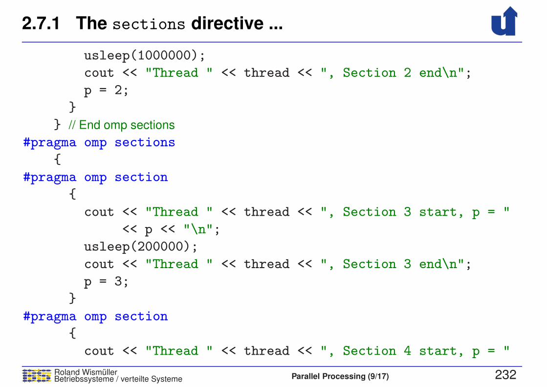
2.7.1 The sections directive ...
Roland WismullerBetriebssysteme / verteilte Systeme Parallel Processing (9/17) 232
usleep(1000000);
cout << "Thread " << thread << ", Section 2 end\n";
p = 2;
}
} // End omp sections
#pragma omp sections
{
#pragma omp section
{
cout << "Thread " << thread << ", Section 3 start, p = "
<< p << "\n";
usleep(200000);
cout << "Thread " << thread << ", Section 3 end\n";
p = 3;
}
#pragma omp section
{
cout << "Thread " << thread << ", Section 4 start, p = "

2.7.1 The sections directive ...
Roland WismullerBetriebssysteme / verteilte Systeme Parallel Processing (9/17) 233
<< p << "\n";
usleep(200000);
cout << "Thread " << thread << ", Section 4 end\n";
p = 4;
}
#pragma omp section
{
cout << "Thread " << thread << ", Section 5 start, p = "
<< p << "\n";
usleep(200000);
cout << "Thread " << thread << ", Section 5 end\n";
p = 5;
}
} // End omp sections
} // End omp parallel
}

2.7.1 The sections directive ...
Roland WismullerBetriebssysteme / verteilte Systeme Parallel Processing (9/17) 234
Example: influence of nowait ...
➥ Executions of the program without nowait option:
Sect. 1 Sect. 2Sect. 1 Sect. 2
Thread 2Thread 1 Thread 3Thread 2Thread 1
Sect. 3p = 1
Sect. 5p = 3
Sect. 4p = 2
Sect. 3p = 1
Sect. 4p = 2
Sect. 5p = −42
BarrierBarrier
Barrier
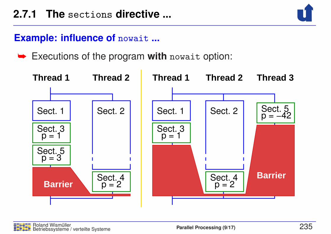
2.7.1 The sections directive ...
Roland WismullerBetriebssysteme / verteilte Systeme Parallel Processing (9/17) 235
Example: influence of nowait ...
➥ Executions of the program with nowait option:
Sect. 1 Sect. 1
Thread 2Thread 1 Thread 3Thread 2Thread 1
Sect. 5p = 3
Sect. 3p = 1
Sect. 4p = 2
Sect. 3p = 1
Sect. 4p = 2
Sect. 5p = −42
Sect. 2 Sect. 2
BarrierBarrier

2.7 Task Parallelism with OpenMP ...
Roland WismullerBetriebssysteme / verteilte Systeme Parallel Processing (9/17) 236
2.7.2 The task Directive: Explicit Tasks
<clause_list>][#pragma omp task
Statement/Block
➥ Creates an explicit task from the statement / the block
➥ Tasks will be executed by the available threads (work pool model)
➥ Options private, firstprivate, shared determine, which
variables belong to the data environment of the task
➥ Option if allows to determine, when an explicit task should be
created
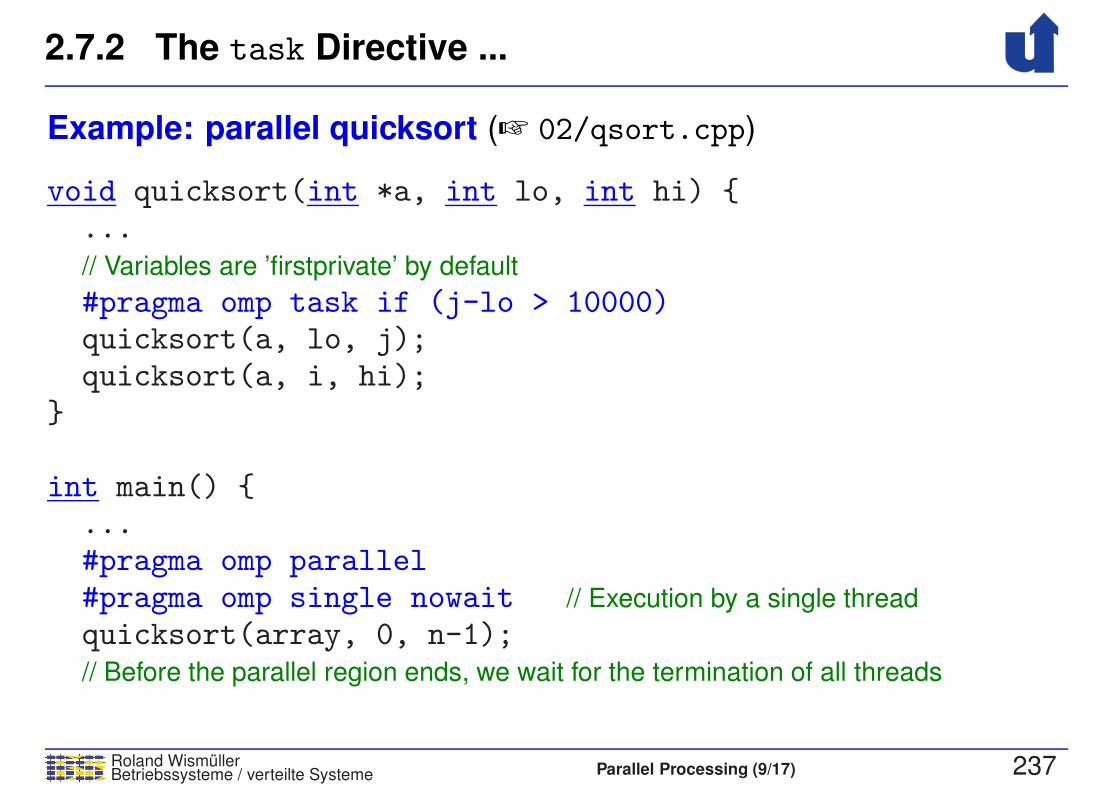
2.7.2 The task Directive ...
Roland WismullerBetriebssysteme / verteilte Systeme Parallel Processing (9/17) 237
Example: parallel quicksort (☞ 02/qsort.cpp)
void quicksort(int *a, int lo, int hi) {...// Variables are ’firstprivate’ by default
#pragma omp task if (j-lo > 10000)quicksort(a, lo, j);quicksort(a, i, hi);
}
int main() {...#pragma omp parallel#pragma omp single nowait // Execution by a single thread
quicksort(array, 0, n-1);// Before the parallel region ends, we wait for the termination of all threads

2.7.2 The task Directive ...
Roland WismullerBetriebssysteme / verteilte Systeme Parallel Processing (9/17) 238
Task synchronization
#pragma omp taskwait #pragma omp taskgroup{
Block}
➥ taskwait: waits for the completion of all direct subtasks of the
current task
➥ taskgroup: at the end of the block, the program waits for all
subtasks (direct and indirect ones), which the current task has
been created within the block
➥ available since OpenMP 4.0
➥ caution: older compilers ignore this directive!
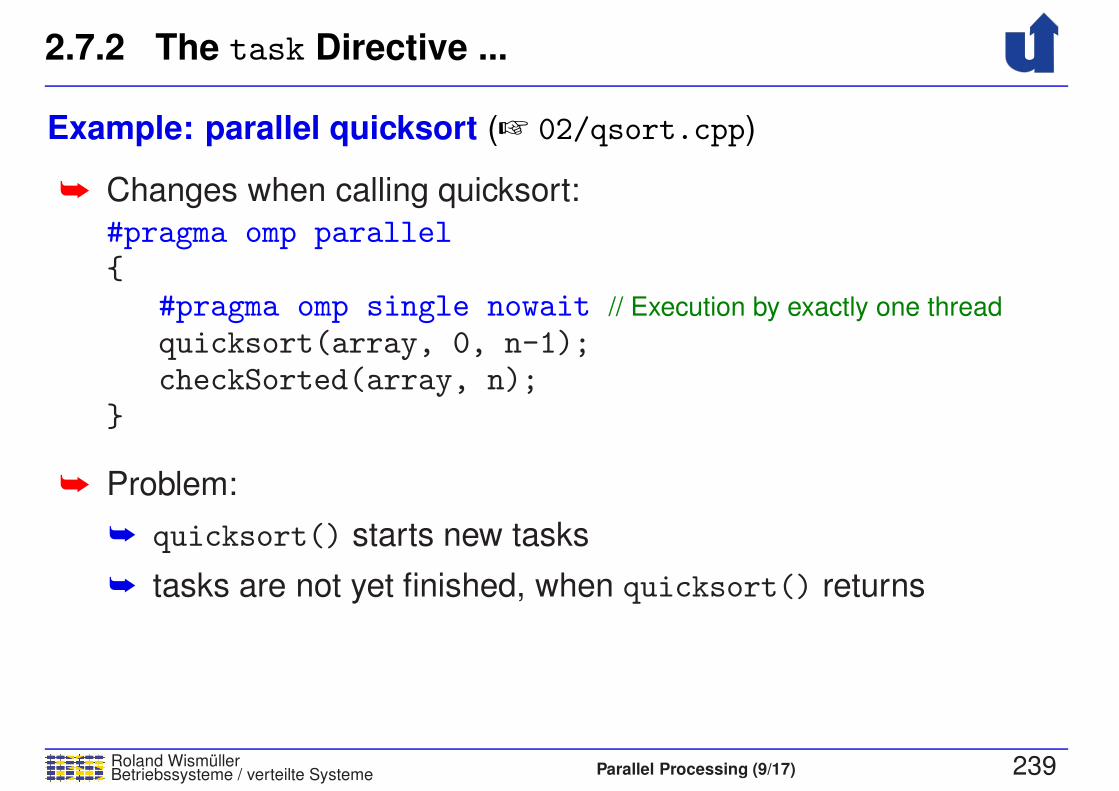
2.7.2 The task Directive ...
Roland WismullerBetriebssysteme / verteilte Systeme Parallel Processing (9/17) 239
Example: parallel quicksort (☞ 02/qsort.cpp)
➥ Changes when calling quicksort:
#pragma omp parallel{
#pragma omp single nowait // Execution by exactly one thread
quicksort(array, 0, n-1);checkSorted(array, n);
}
➥ Problem:
➥ quicksort() starts new tasks
➥ tasks are not yet finished, when quicksort() returns
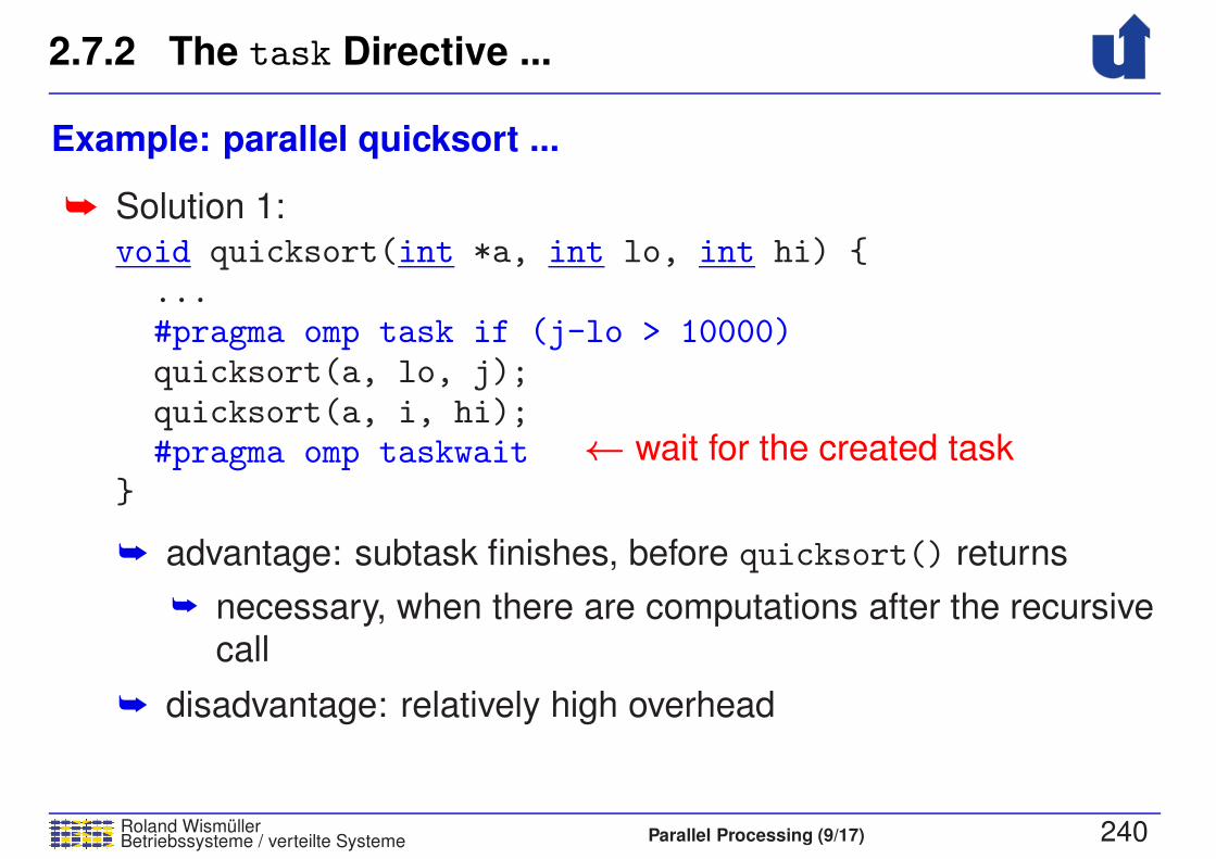
2.7.2 The task Directive ...
Roland WismullerBetriebssysteme / verteilte Systeme Parallel Processing (9/17) 240
Example: parallel quicksort ...
➥ Solution 1:
← wait for the created task
void quicksort(int *a, int lo, int hi) {...#pragma omp task if (j-lo > 10000)quicksort(a, lo, j);quicksort(a, i, hi);#pragma omp taskwait
}
➥ advantage: subtask finishes, before quicksort() returns
➥ necessary, when there are computations after the recursivecall
➥ disadvantage: relatively high overhead
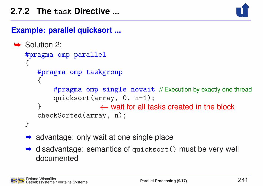
2.7.2 The task Directive ...
Roland WismullerBetriebssysteme / verteilte Systeme Parallel Processing (9/17) 241
Example: parallel quicksort ...
➥ Solution 2:
← wait for all tasks created in the block
#pragma omp parallel{
#pragma omp taskgroup{
#pragma omp single nowait // Execution by exactly one thread
quicksort(array, 0, n-1);}checkSorted(array, n);
}
➥ advantage: only wait at one single place
➥ disadvantage: semantics of quicksort() must be very well
documented
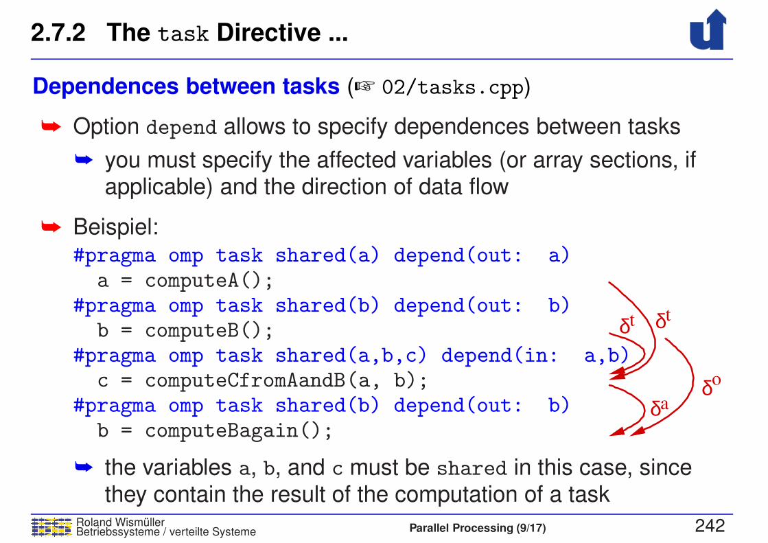
2.7.2 The task Directive ...
Roland WismullerBetriebssysteme / verteilte Systeme Parallel Processing (9/17) 242
Dependences between tasks (☞ 02/tasks.cpp)
➥ Option depend allows to specify dependences between tasks
➥ you must specify the affected variables (or array sections, ifapplicable) and the direction of data flow
➥ Beispiel:
δ δ
δa
tt
δo
#pragma omp task shared(a) depend(out: a)a = computeA();
#pragma omp task shared(b) depend(out: b)b = computeB();
#pragma omp task shared(a,b,c) depend(in: a,b)c = computeCfromAandB(a, b);
#pragma omp task shared(b) depend(out: b)b = computeBagain();
➥ the variables a, b, and c must be shared in this case, sincethey contain the result of the computation of a task
2.8 OpenMP Details
Roland WismullerBetriebssysteme / verteilte Systeme Parallel Processing (9/17) 243
2.8.1 Thread Affinity
➥ Goal: control where threads are executed
➥ i.e., by which HW threads on which core on which CPU
➥ Important (among others) because of the architecture of today’s
multicore CPUs
➥ HW threads share the functional units of a core
➥ cores share the L2 caches and the memory interface
➥ Concept of OpenMP:
➥ introduction of places
➥ place: set of hardware execution environments
➥ e.g., hardware thread, core, processor (socket)
➥ options control the distribution from threads to places
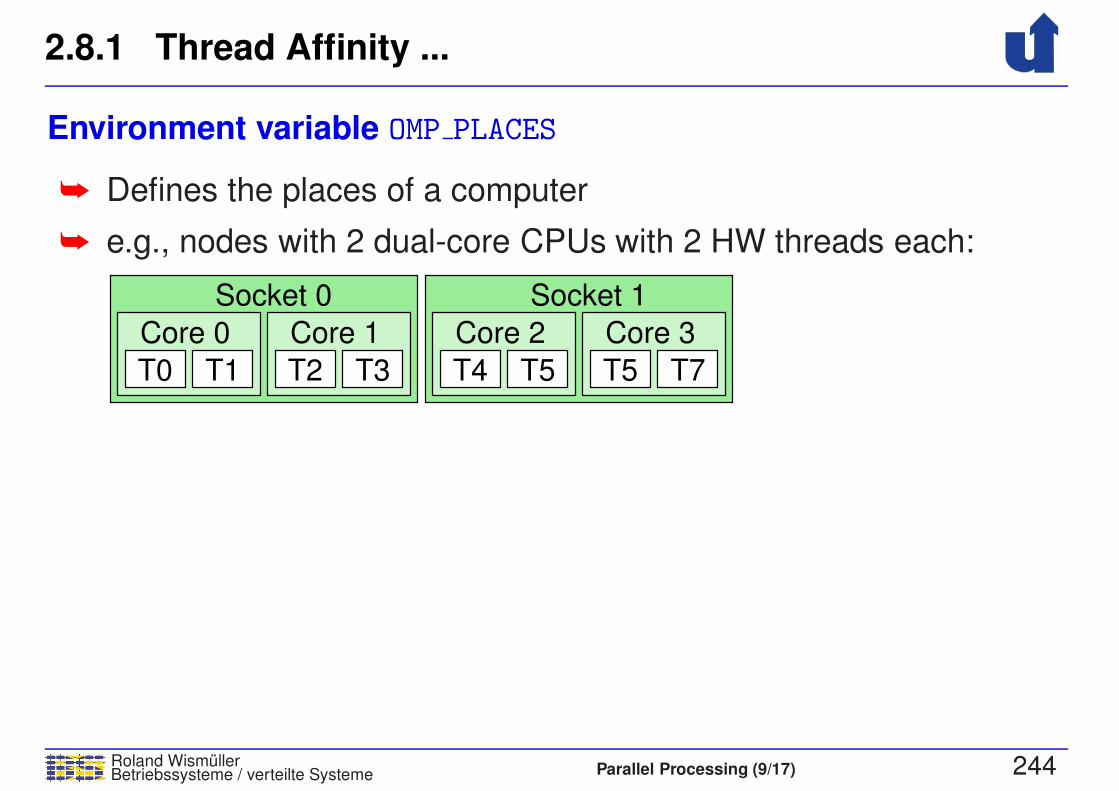
2.8.1 Thread Affinity ...
Roland WismullerBetriebssysteme / verteilte Systeme Parallel Processing (9/17) 244
Environment variable OMP PLACES
➥ Defines the places of a computer
➥ e.g., nodes with 2 dual-core CPUs with 2 HW threads each:
T2 T3
Core 1
T4 T5
Core 2
T5 T7
Core 3
T0 T1
Core 0
Socket 0 Socket 1
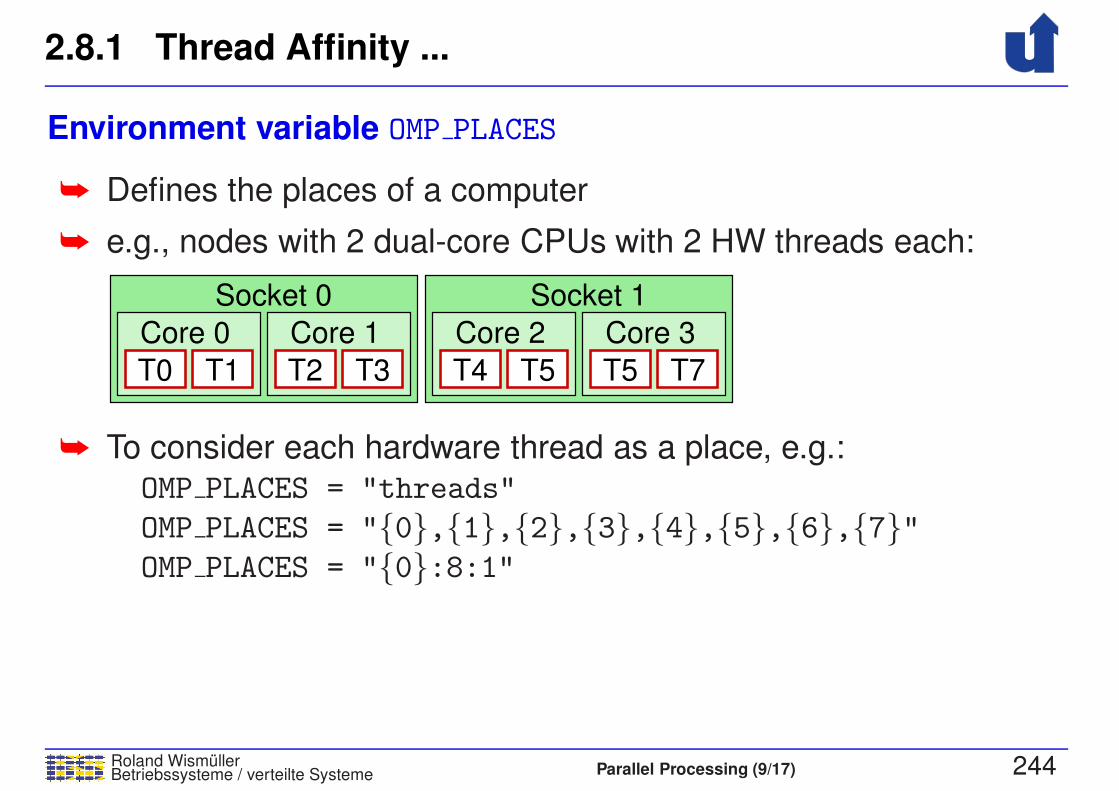
➥ To consider each hardware thread as a place, e.g.:
OMP PLACES = "threads"
OMP PLACES = "{0},{1},{2},{3},{4},{5},{6},{7}"OMP PLACES = "{0}:8:1"
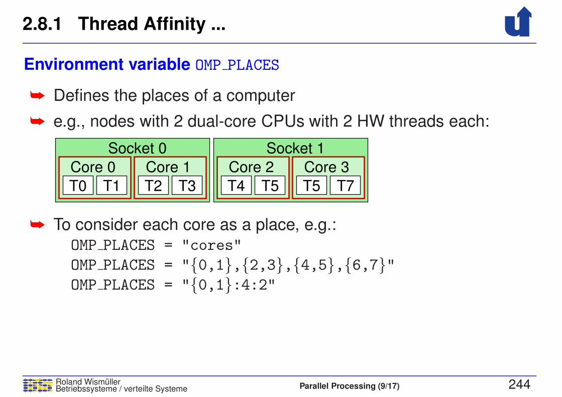
2.8.1 Thread Affinity ...
Roland WismullerBetriebssysteme / verteilte Systeme Parallel Processing (9/17) 244
Environment variable OMP PLACES
➥ Defines the places of a computer
➥ e.g., nodes with 2 dual-core CPUs with 2 HW threads each:
T2 T3
Core 1
T4 T5
Core 2
T5 T7
Core 3
T0 T1
Core 0
Socket 0 Socket 1
➥ To consider each core as a place, e.g.:
OMP PLACES = "cores"
OMP PLACES = "{0,1},{2,3},{4,5},{6,7}"OMP PLACES = "{0,1}:4:2"

2.8.1 Thread Affinity ...
Roland WismullerBetriebssysteme / verteilte Systeme Parallel Processing (9/17) 244
Environment variable OMP PLACES
➥ Defines the places of a computer
➥ e.g., nodes with 2 dual-core CPUs with 2 HW threads each:
T2 T3
Core 1
T4 T5
Core 2
T5 T7
Core 3
T0 T1
Core 0
Socket 0 Socket 1
➥ To consider each socket as a place, e.g.:
OMP PLACES = "sockets"
OMP PLACES = "sockets(2)"
OMP PLACES = "{0:4},{4:4}"

2.8.1 Thread Affinity ...
Roland WismullerBetriebssysteme / verteilte Systeme Parallel Processing (9/17) 245
Mapping from threads to places
➥ Option proc bind( spread | close | master ) of the
parallel directive
➥ spread: threads will be evenly distributed to the available
places; the list of places will be partitioned
➥ avoids resource conflicts between threads
➥ close: threads are allocated as close to the master thread as
possible
➥ e.g., to make optimal use ot the shared cache
➥ master: threads will be allocated on the same place as the
master thread
➥ closest possible locality to master thread
➥ Usually combined with nested parallel regions

Roland WismullerBetriebssysteme / verteilte Systeme Parallel Processing (10/17) xi
Roland Wismuller
Universitat Siegen
Tel.: 0271/740-4050, Buro: H-B 8404
Stand: January 23, 2018
Parallel Processing
WS 2017/18
11.12.2017
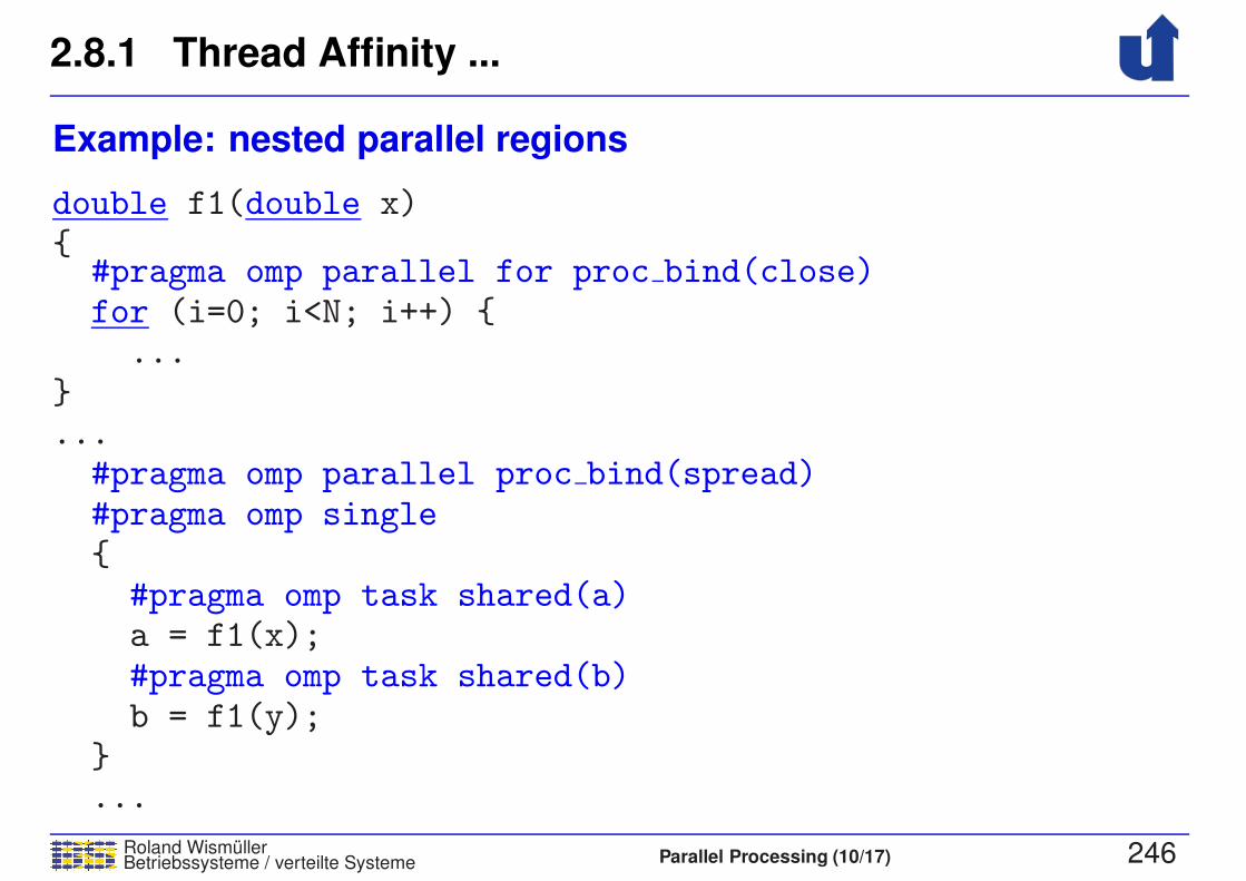
2.8.1 Thread Affinity ...
Roland WismullerBetriebssysteme / verteilte Systeme Parallel Processing (10/17) 246
Example: nested parallel regions
double f1(double x){
#pragma omp parallel for proc bind(close)for (i=0; i<N; i++) {...
}...
#pragma omp parallel proc bind(spread)#pragma omp single{#pragma omp task shared(a)a = f1(x);#pragma omp task shared(b)b = f1(y);
}...
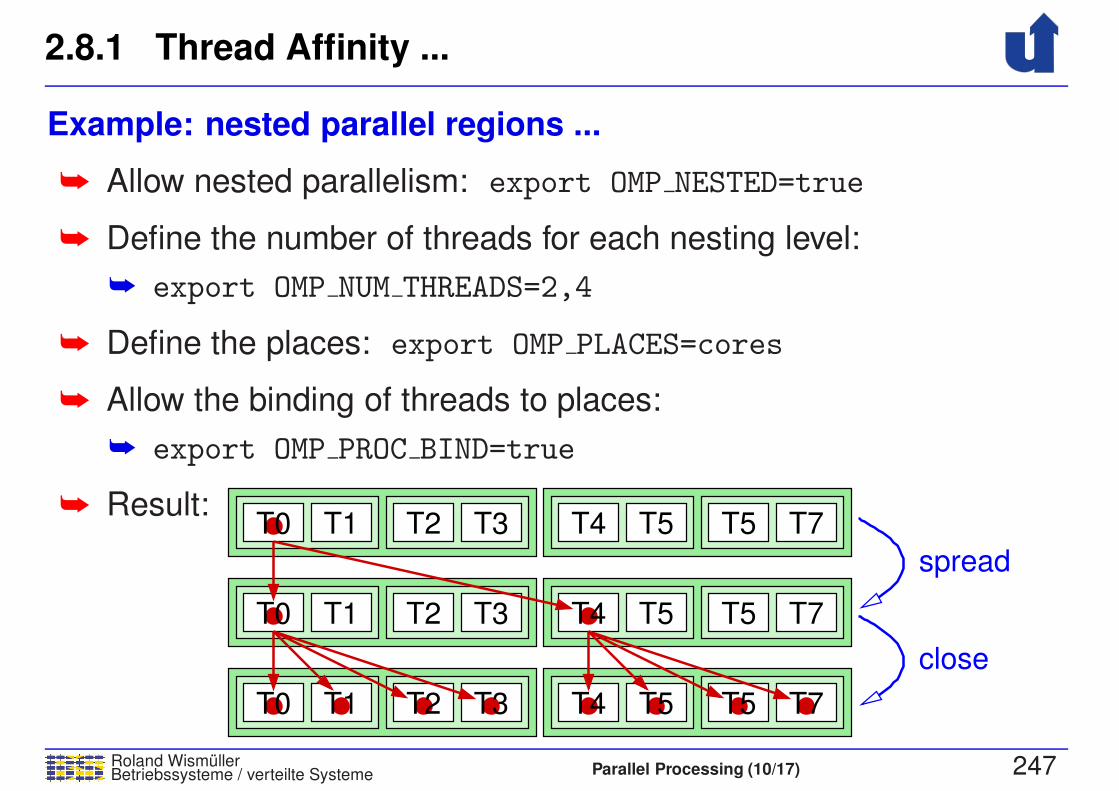
2.8.1 Thread Affinity ...
Roland WismullerBetriebssysteme / verteilte Systeme Parallel Processing (10/17) 247
Example: nested parallel regions ...
➥ Allow nested parallelism: export OMP NESTED=true
➥ Define the number of threads for each nesting level:
➥ export OMP NUM THREADS=2,4
➥ Define the places: export OMP PLACES=cores
➥ Allow the binding of threads to places:
➥ export OMP PROC BIND=true
➥ Result:T4 T5T2 T3 T5 T7T0 T1
T4 T5T2 T3 T5 T7T0 T1
T4 T5T2 T3 T5 T7T0 T1
spread
close

2.8 OpenMP Details ...
Roland WismullerBetriebssysteme / verteilte Systeme Parallel Processing (10/17) 248
2.8.2 SIMD Vectorization
<clause_list>][
for(...) ...
#pragma omp simd
➥ Restructuring of a loop in order to use the SIMD vector registers
➥ e.g., Intel SSE: 4 float operations in parallel
➥ Loop will be executed by a sinlge thread
➥ combination with for is possible
➥ Options (among others): private, lastprivate, reduction
➥ Option safelen: maximum vector length
➥ i.e., distance (in iterations) of data dependences, e.g.:
for (i=0; i<N; i++)
a[i] = b[i] + a[i-4]; // safelen = 4
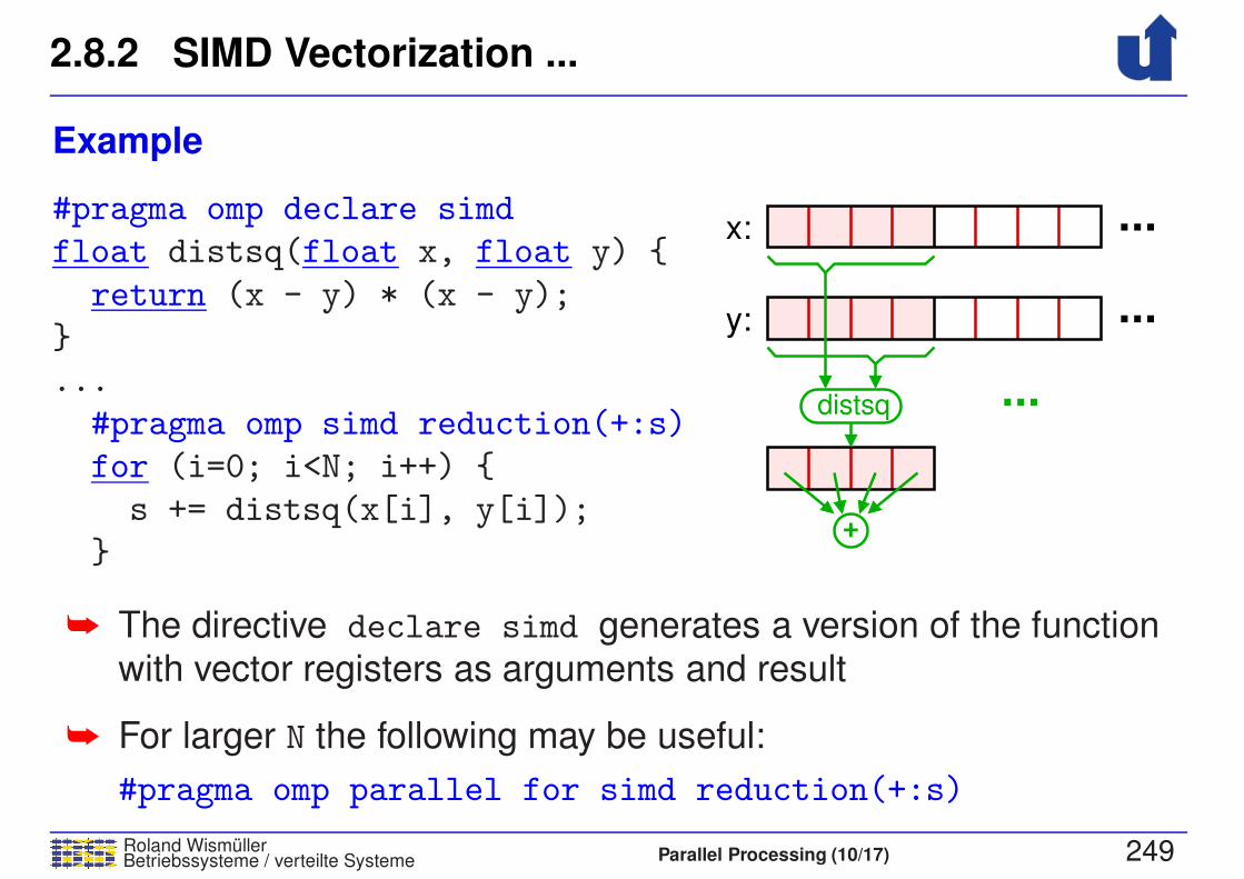
2.8.2 SIMD Vectorization ...
Roland WismullerBetriebssysteme / verteilte Systeme Parallel Processing (10/17) 249
Example
...
...
...
x:
y:
distsq
+
#pragma omp declare simd
float distsq(float x, float y) {
return (x - y) * (x - y);
}
...
#pragma omp simd reduction(+:s)
for (i=0; i<N; i++) {
s += distsq(x[i], y[i]);
}
➥ The directive declare simd generates a version of the functionwith vector registers as arguments and result
➥ For larger N the following may be useful:
#pragma omp parallel for simd reduction(+:s)
2.8 OpenMP Details ...
Roland WismullerBetriebssysteme / verteilte Systeme Parallel Processing (10/17) 250
2.8.3 Using External Accelerators
➥ Model in OpenMP 4.0:
➥ one host (multi processor with shared memory)
with several identical accelerators (targets)
➥ execution of a code block can be moved to a target using a
directive
➥ host and target can have a shared memory, but this is not
required
➥ data transport must be executed using directives
➥ In order to support the execution model of GPUs:
➥ introduction of thread teams
➥ threads of the same team are executed by one streamingmultiprocessor (in SIMD manner)

2.8.3 Using External Accelerators ...
Roland WismullerBetriebssysteme / verteilte Systeme Parallel Processing (10/17) 251
The target directive
<clause_list>][#pragma omp target [ data ]
➥ Transfers execution and data to a target
➥ data will be copied between CPU memory and target memory
➥ mapping and direction of transfer are specified using themap option
➥ the subsequent code block will be executed on the target
➥ except when only a data environment is created using
target data
➥ Host waits until the computation on the target is finished
➥ however, the target directive is also possible within an
asynchronous task
2.8.3 Using External Accelerators ...
Roland WismullerBetriebssysteme / verteilte Systeme Parallel Processing (10/17) 252
The map option
➥ Maps variable vH in the host data environment to the
corresponding variable vT in the target data environment
➥ either the data is copied between vH and vT
or vH and vT are identical
➥ Syntax: map( alloc | to | from | tofrom : <list> )
➥ <list>: list of the original variables
➥ array sections are allowed, too, ☞ 2.7.2
➥ alloc: just allocate memory for vT
➥ to: allocate vT , copy vH to vT at the beginning
➥ from: allocate vT , copy vT to vH at the end
➥ tofrom: default value, to and from
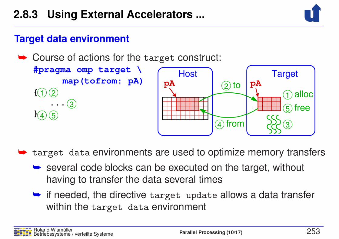
2.8.3 Using External Accelerators ...
Roland WismullerBetriebssysteme / verteilte Systeme Parallel Processing (10/17) 253
Target data environment
➥ Course of actions for the target construct:
pA pAHost
#pragma omp target \
map(tofrom: pA)
{
...
}
to
from
alloc
free
Target
2
4
1 2
3
4 53
1
5
➥ target data environments are used to optimize memory transfers
➥ several code blocks can be executed on the target, without
having to transfer the data several times
➥ if needed, the directive target update allows a data transfer
within the target data environment
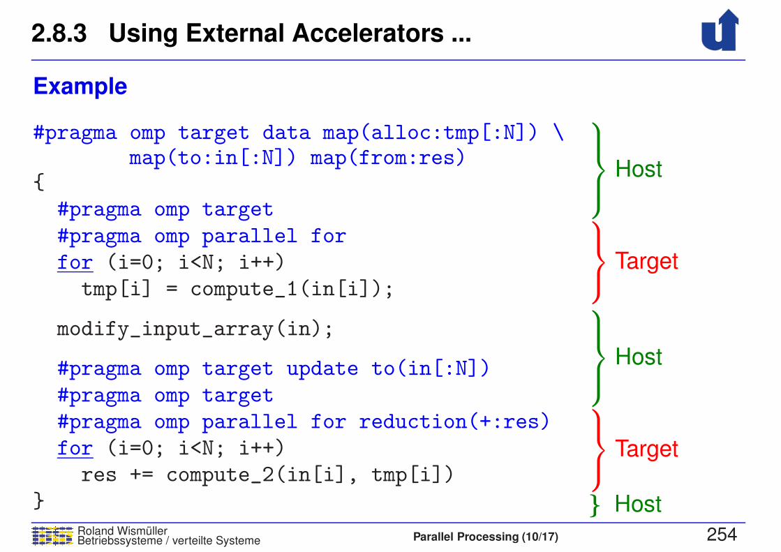
2.8.3 Using External Accelerators ...
Roland WismullerBetriebssysteme / verteilte Systeme Parallel Processing (10/17) 254
Example
Host
Target
Host
Target
} Host
#pragma omp target data map(alloc:tmp[:N]) \map(to:in[:N]) map(from:res)
{#pragma omp target
#pragma omp parallel forfor (i=0; i<N; i++)tmp[i] = compute_1(in[i]);
modify_input_array(in);
#pragma omp target update to(in[:N])
#pragma omp target#pragma omp parallel for reduction(+:res)for (i=0; i<N; i++)res += compute_2(in[i], tmp[i])
}

2.8.3 Using External Accelerators ...
Roland WismullerBetriebssysteme / verteilte Systeme Parallel Processing (10/17) 255
Thread teams
➥ Allow a parallelization at two levels, e.g., on GPUs
➥ Create a set of thread teams:
<clause_list>][
Statement/Block
#pragma omp teams
➥ statement/block is executed by the master thread of each team
➥ teams can not synchronize
➥ Distribution of a loop to the master threads of the teams:
<clause_list>][
for(...) ...
#pragma omp distribute
➥ Parallelization within a team, e.g., using parallel for

2.8.3 Using External Accelerators ...
Roland WismullerBetriebssysteme / verteilte Systeme Parallel Processing (10/17) 256
Example: SAXPY
➥ On the host:
void saxpy(float *y, float *x, float a, int n) {#pragma omp parallel for
for (int i = 0; i < n; i++)y[i] = a*x[i] + y[i];
}
➥ On the GPU (naive):
void saxpy(float *y, float *x, float a, int n) {
#pragma omp target map(to:x[0:n], n, a) map(y[0:n]){#pragma omp parallel forfor (int i = 0; i < n; i++)
y[i] = a*x[i] + y[i];}
}

2.8.3 Using External Accelerators ...
Roland WismullerBetriebssysteme / verteilte Systeme Parallel Processing (10/17) 257
Example: SAXPY ...
➥ On the GPU (optimized): each team processes a block
void saxpy(float *y, float *x, float a, int n) {int nBlk = numBlocks(n); // Number of blocks
int nThr = numThreads(n); // Number of threads
#pragma omp target map(to:x[0:n], n, a) map(y[0:n])#pragma omp teams num teams(nBlk) thread limit(nThr){#pragma omp distributefor (int i = 0; i < n; i += n/nBlk) {
#pragma omp parallel forfor (int j = i; j < i + n/nBlk; j++)y[j] = a*x[j] + y[j];
}}
}}
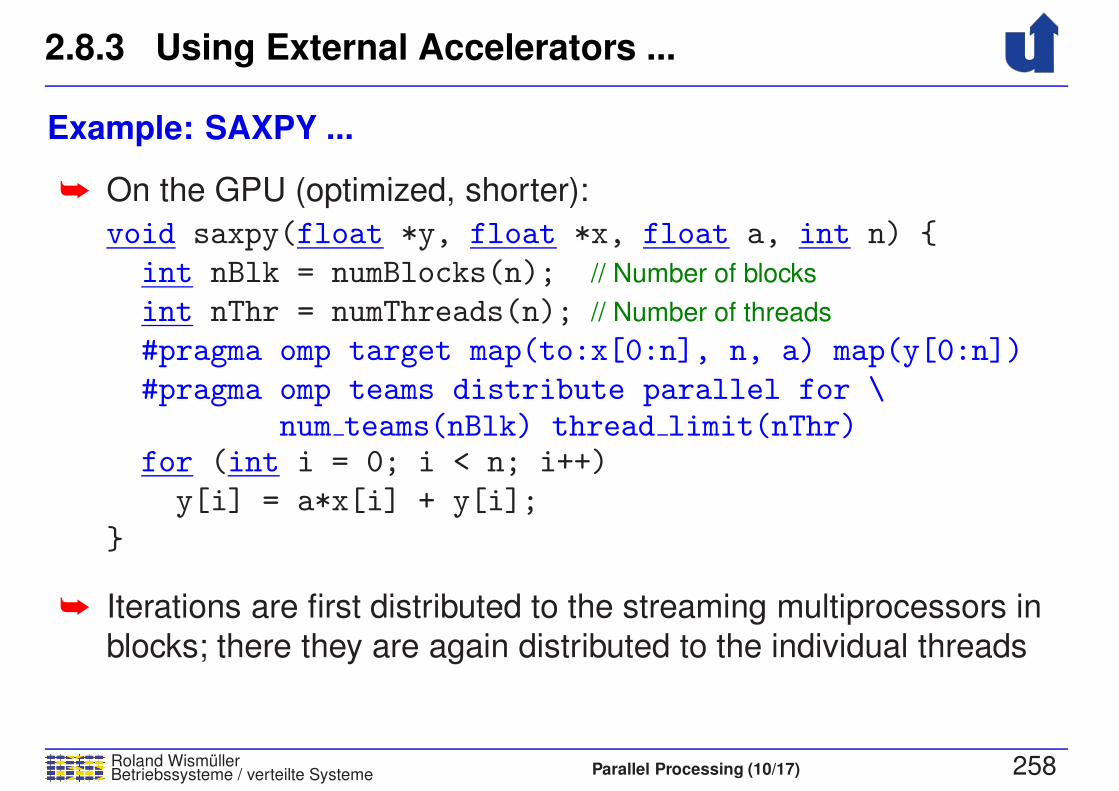
2.8.3 Using External Accelerators ...
Roland WismullerBetriebssysteme / verteilte Systeme Parallel Processing (10/17) 258
Example: SAXPY ...
➥ On the GPU (optimized, shorter):
void saxpy(float *y, float *x, float a, int n) {
int nBlk = numBlocks(n); // Number of blocks
int nThr = numThreads(n); // Number of threads
#pragma omp target map(to:x[0:n], n, a) map(y[0:n])
#pragma omp teams distribute parallel for \num teams(nBlk) thread limit(nThr)
for (int i = 0; i < n; i++)
y[i] = a*x[i] + y[i];
}
➥ Iterations are first distributed to the streaming multiprocessors in
blocks; there they are again distributed to the individual threads
Roland WismullerBetriebssysteme / verteilte Systeme Parallel Processing (10/17) 259
Parallel ProcessingWS 2017/18
3 Parallel Programming with Message Passing
3 Parallel Programming with Message Passing ...
Roland WismullerBetriebssysteme / verteilte Systeme Parallel Processing (10/17) 260
Contents
➥ Typical approach
➥ MPI (Message Passing Interface)
➥ core routines
➥ simple MPI programs
➥ point-to-point communication
➥ complex data types in messages
➥ communicators
➥ collective operations
➥ further concepts
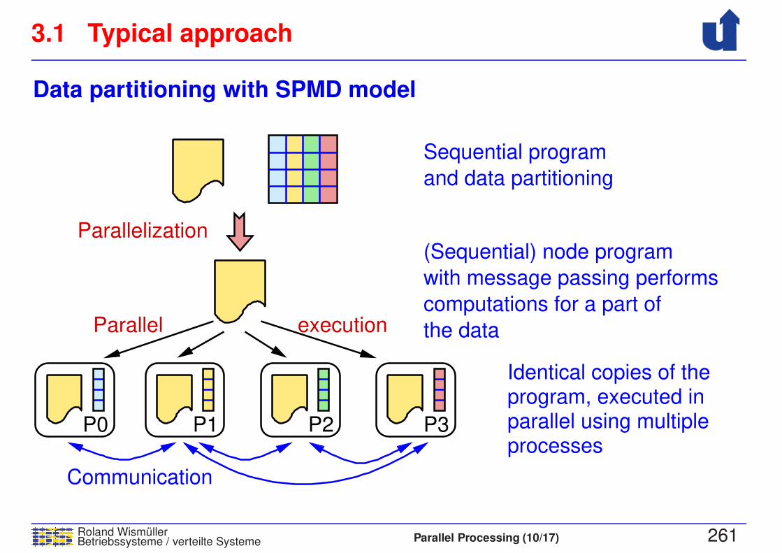
3.1 Typical approach
Roland WismullerBetriebssysteme / verteilte Systeme Parallel Processing (10/17) 261
Data partitioning with SPMD model
P0 P1 P2 P3
Communication
Sequential program
and data partitioning
with message passing performs
(Sequential) node program
computations for a part of
the data
Identical copies of theprogram, executed inparallel using multipleprocesses
Parallelization
Parallel execution
3.1 Typical approach ...
Roland WismullerBetriebssysteme / verteilte Systeme Parallel Processing (10/17) 262
Activities when creating a node program
➥ Adjustment of array declarations
➥ node program stores only a part of the data
➥ (assumption: data are stored in arrays)
➥ Index transformation
➥ global index↔ (process number, local index)
➥ Work partitioning
➥ each process executes the computations on its part of the data
➥ Communication
➥ when a process needs non-local data, a suitable message
exchange must be programmed
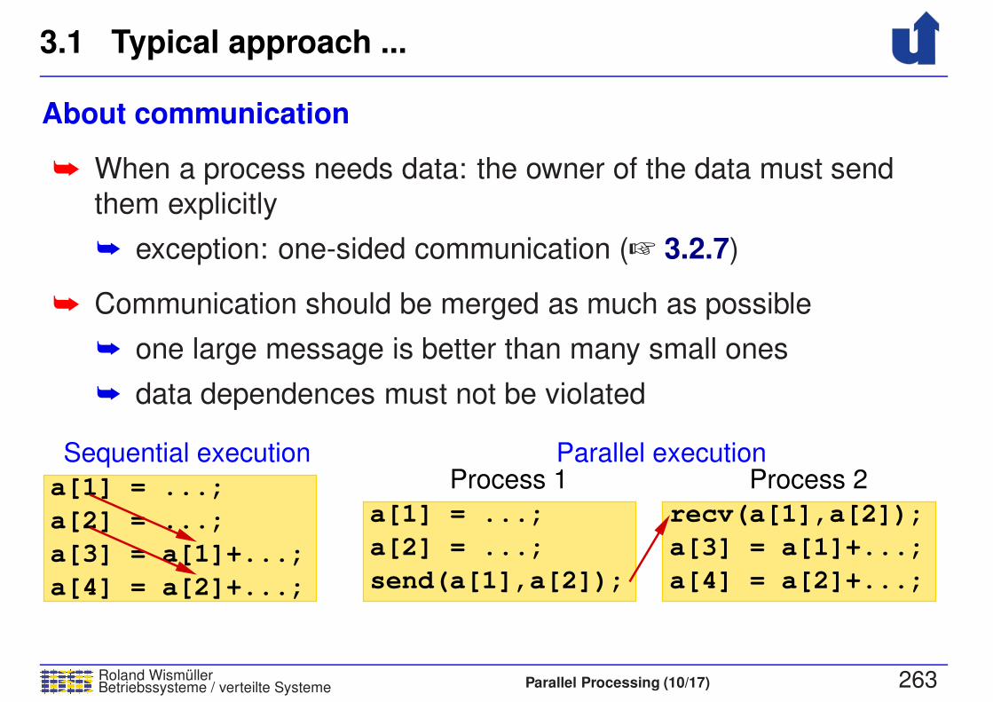
3.1 Typical approach ...
Roland WismullerBetriebssysteme / verteilte Systeme Parallel Processing (10/17) 263
About communication
➥ When a process needs data: the owner of the data must send
them explicitly
➥ exception: one-sided communication (☞ 3.2.7)
➥ Communication should be merged as much as possible
➥ one large message is better than many small ones
➥ data dependences must not be violated
a[4] = a[2]+...;
a[3] = a[1]+...;
recv(a[1],a[2]);
Process 2
send(a[1],a[2]);
a[2] = ...;
a[1] = ...;
Process 1Sequential execution Parallel execution
a[1] = ...;
a[2] = ...;
a[3] = a[1]+...;
a[4] = a[2]+...;
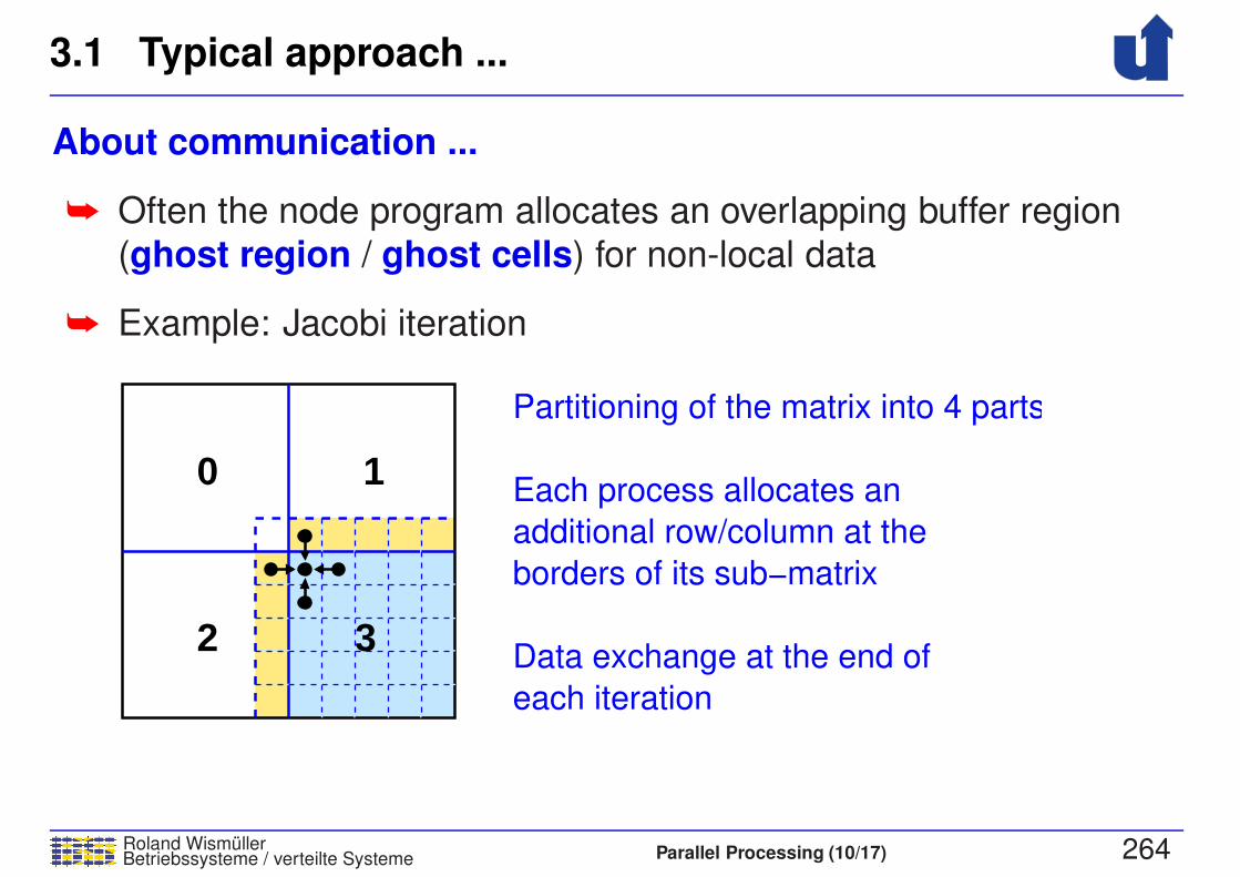
3.1 Typical approach ...
Roland WismullerBetriebssysteme / verteilte Systeme Parallel Processing (10/17) 264
About communication ...
➥ Often the node program allocates an overlapping buffer region
(ghost region / ghost cells) for non-local data
➥ Example: Jacobi iteration
Partitioning of the matrix into 4 parts
Each process allocates an
Data exchange at the end of
each iteration
additional row/column at the
borders of its sub−matrix
0 1
32
3.2 MPI (Message Passing Interface)
Roland WismullerBetriebssysteme / verteilte Systeme Parallel Processing (10/17) 265
History and background
➥ At the beginning of the parallel computer era (late 1980’s):
➥ many different communication libraries (NX, PARMACS, PVM,P4, ...)
➥ parallel programs are not easily portable
➥ Definition of an informal standard by the MPI forum
➥ 1994: MPI-1.0
➥ 1997: MPI-1.2 and MPI-2.0 (considerable extensions)
➥ 2009: MPI 2.2 (clarifications, minor extensions)
➥ 2012/15: MPI-3.0 und MPI-3.1 (considerable extensions)
➥ documents at http://www.mpi-forum.org/docs
➥ MPI only defines the API (i.e., the programming interface)
➥ different implementations, e.g., MPICH2, OpenMPI, ...
3.2 MPI (Message Passing Interface) ...
Roland WismullerBetriebssysteme / verteilte Systeme Parallel Processing (10/17) 266
Programming model
➥ Distributed memory, processes with message passing
➥ SPMD: one program code for all processes
➥ but different program codes are also possible
➥ MPI-1: static process model
➥ all processes are created at program start
➥ program start is standardized since MPI-2
➥ MPI-2 also allows to create new processes at runtime
➥ MPI is thread safe: a process is allowed to create additionalthreads
➥ hybrid parallelization using MPI and OpenMP is possible
➥ Program terminates when all its processes have terminated
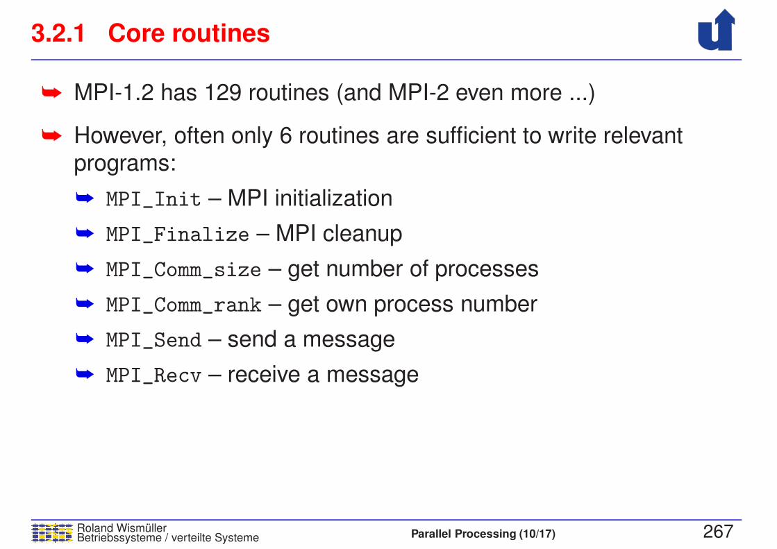
3.2.1 Core routines
Roland WismullerBetriebssysteme / verteilte Systeme Parallel Processing (10/17) 267
➥ MPI-1.2 has 129 routines (and MPI-2 even more ...)
➥ However, often only 6 routines are sufficient to write relevant
programs:
➥ MPI_Init – MPI initialization
➥ MPI_Finalize – MPI cleanup
➥ MPI_Comm_size – get number of processes
➥ MPI_Comm_rank – get own process number
➥ MPI_Send – send a message
➥ MPI_Recv – receive a message
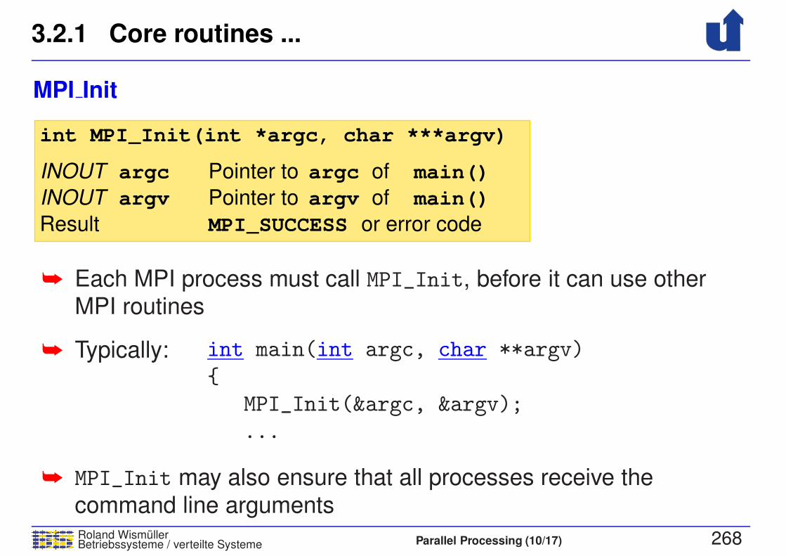
3.2.1 Core routines ...
Roland WismullerBetriebssysteme / verteilte Systeme Parallel Processing (10/17) 268
MPI Init
INOUT
INOUT
Pointer to argc of main()
Pointer to argv of main()
MPI_SUCCESS or error code
int MPI_Init(int *argc, char ***argv)
Result
argc
argv
➥ Each MPI process must call MPI_Init, before it can use otherMPI routines
➥ Typically: int main(int argc, char **argv)
{
MPI_Init(&argc, &argv);
...
➥ MPI_Init may also ensure that all processes receive the
command line arguments
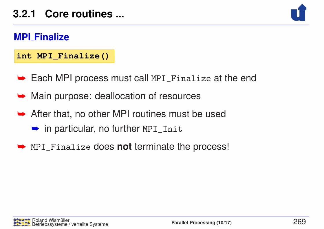
3.2.1 Core routines ...
Roland WismullerBetriebssysteme / verteilte Systeme Parallel Processing (10/17) 269
MPI Finalize
int MPI_Finalize()
➥ Each MPI process must call MPI_Finalize at the end
➥ Main purpose: deallocation of resources
➥ After that, no other MPI routines must be used
➥ in particular, no further MPI_Init
➥ MPI_Finalize does not terminate the process!
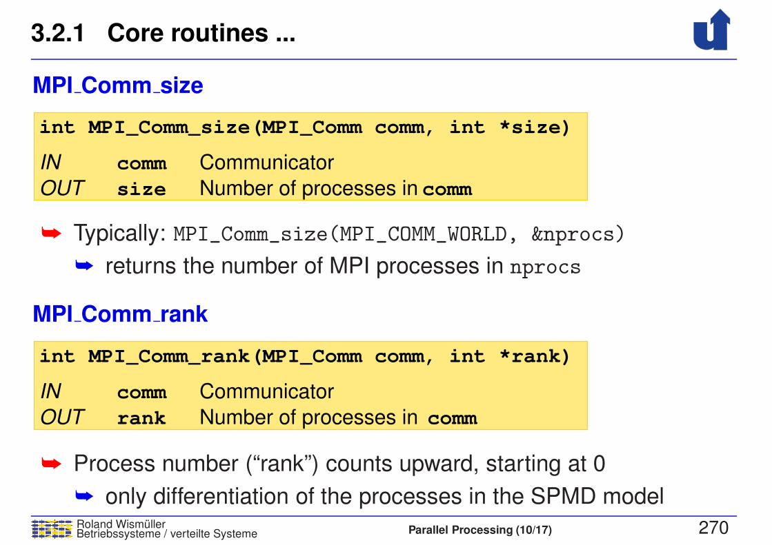
3.2.1 Core routines ...
Roland WismullerBetriebssysteme / verteilte Systeme Parallel Processing (10/17) 270
MPI Comm size
int MPI_Comm_size(MPI_Comm comm, int *size)
comm
size comm
IN
OUT
Communicator
Number of processes in
➥ Typically: MPI_Comm_size(MPI_COMM_WORLD, &nprocs)
➥ returns the number of MPI processes in nprocs
MPI Comm rank
comm
int MPI_Comm_rank(MPI_Comm comm, int *rank)
rank
Communicator
Number of processes in OUT
IN
comm
➥ Process number (“rank”) counts upward, starting at 0
➥ only differentiation of the processes in the SPMD model
3.2.1 Core routines ...
Roland WismullerBetriebssysteme / verteilte Systeme Parallel Processing (10/17) 271
Communicators
➥ A communicator consists of
➥ a process group
➥ a subset of all processes of the parallel application
➥ a communication context
➥ to allow the separation of different communication relations
(☞ 3.2.5)
➥ There is a predefined communicator MPI_COMM_WORLD
➥ its process group contains all processes of the parallel
application
➥ Additional communicators can be created as needed (☞ 3.2.5)

Roland WismullerBetriebssysteme / verteilte Systeme Parallel Processing (11/17) xii
Roland Wismuller
Universitat Siegen
Tel.: 0271/740-4050, Buro: H-B 8404
Stand: January 23, 2018
Parallel Processing
WS 2017/18
18.12.2017
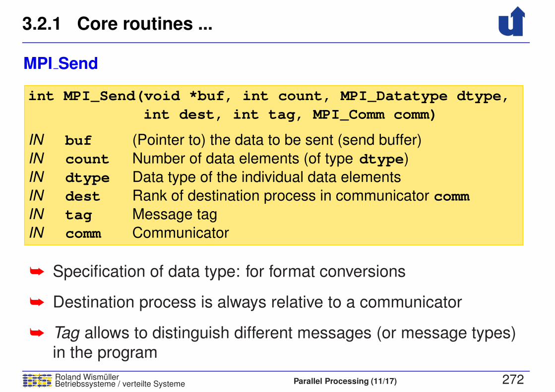
3.2.1 Core routines ...
Roland WismullerBetriebssysteme / verteilte Systeme Parallel Processing (11/17) 272
MPI Send
IN
)
int MPI_Send(void *buf, int count, MPI_Datatype dtype,
int dest, int tag, MPI_Comm comm)
comm
tag
dest
count
buf
dtype
IN
IN
IN
IN
IN Communicator
Message tag
Data type of the individual data elements
Number of data elements (of type
(Pointer to) the data to be sent (send buffer)
Rank of destination process in communicator
dtype
comm
➥ Specification of data type: for format conversions
➥ Destination process is always relative to a communicator
➥ Tag allows to distinguish different messages (or message types)
in the program

3.2.1 Core routines ...
Roland WismullerBetriebssysteme / verteilte Systeme Parallel Processing (11/17) 273
MPI Send ...
➥ MPI_Send blocks the calling process, until all data has been read
from the send buffer
➥ send buffer can be reused (i.e., modified) immediately after
MPI_Send returns
➥ The MPI implementation decides whether the process is blocked
until
a) the data has been copied to a system buffer, or
b) the data has been received by the destination process.
➥ in some cases, this decision can influence the correctness of
the program! (☞ slide 286)

3.2.1 Core routines ...
Roland WismullerBetriebssysteme / verteilte Systeme Parallel Processing (11/17) 274
MPI Recv
IN
IN
IN
IN
IN
OUT
OUT
comm
tag
count
buf
dtype
source
status
Communicator
Message tag
Data type of the individual data elements
Rank of source process in communicator
int MPI_Recv(void *buf, int count, MPI_Datatype dtype,
int source, int tag, MPI_Comm comm,
MPI_Status *status)
Status (among others: actual message length)
(Pointer to) receive buffer
Buffer size (number of data elements of type
comm
dtype)
➥ Process is blocked until the message has been completely
received and stored in the receive buffer
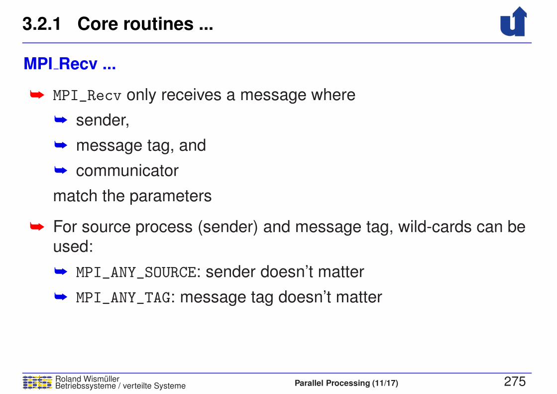
3.2.1 Core routines ...
Roland WismullerBetriebssysteme / verteilte Systeme Parallel Processing (11/17) 275
MPI Recv ...
➥ MPI_Recv only receives a message where
➥ sender,
➥ message tag, and
➥ communicator
match the parameters
➥ For source process (sender) and message tag, wild-cards can be
used:
➥ MPI_ANY_SOURCE: sender doesn’t matter
➥ MPI_ANY_TAG: message tag doesn’t matter
3.2.1 Core routines ...
Roland WismullerBetriebssysteme / verteilte Systeme Parallel Processing (11/17) 276
MPI Recv ...
➥ Message must not be larger than the receive buffer
➥ but it may be smaller; the unused part of the buffer remains
unchanged
➥ From the return value status you can determine:
➥ the sender of the message: status.MPI_SOURCE
➥ the message tag: status.MPI_TAG
➥ the error code: status.MPI_ERROR
➥ the actual length of the received message (number of data
elements): MPI_Get_count(&status, dtype, &count)
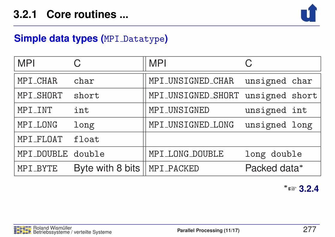
3.2.1 Core routines ...
Roland WismullerBetriebssysteme / verteilte Systeme Parallel Processing (11/17) 277
Simple data types (MPI Datatype)
MPI C MPI C
MPI CHAR char MPI UNSIGNED CHAR unsigned char
MPI SHORT short MPI UNSIGNED SHORT unsigned short
MPI INT int MPI UNSIGNED unsigned int
MPI LONG long MPI UNSIGNED LONG unsigned long
MPI FLOAT float
MPI DOUBLE double MPI LONG DOUBLE long double
MPI BYTE Byte with 8 bits MPI PACKED Packed data∗
∗
☞ 3.2.4
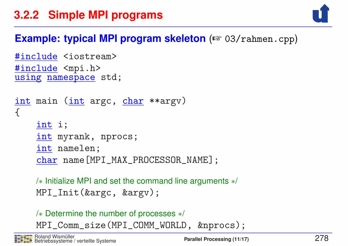
3.2.2 Simple MPI programs
Roland WismullerBetriebssysteme / verteilte Systeme Parallel Processing (11/17) 278
Example: typical MPI program skeleton (☞ 03/rahmen.cpp)
#include <iostream>#include <mpi.h>using namespace std;
int main (int argc, char **argv){
int i;
int myrank, nprocs;int namelen;char name[MPI_MAX_PROCESSOR_NAME];
/∗ Initialize MPI and set the command line arguments ∗/
MPI_Init(&argc, &argv);
/∗ Determine the number of processes ∗/
MPI_Comm_size(MPI_COMM_WORLD, &nprocs);
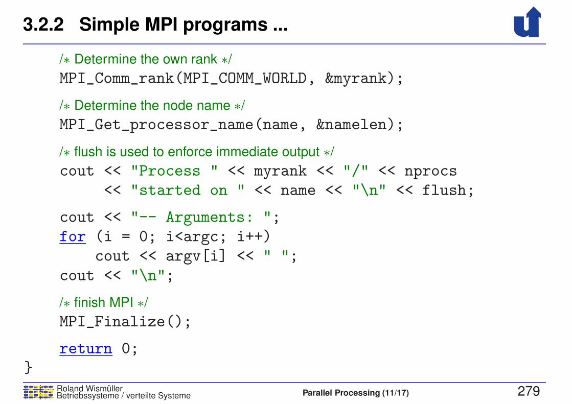
3.2.2 Simple MPI programs ...
Roland WismullerBetriebssysteme / verteilte Systeme Parallel Processing (11/17) 279
/∗ Determine the own rank ∗/
MPI_Comm_rank(MPI_COMM_WORLD, &myrank);
/∗ Determine the node name ∗/
MPI_Get_processor_name(name, &namelen);
/∗ flush is used to enforce immediate output ∗/
cout << "Process " << myrank << "/" << nprocs<< "started on " << name << "\n" << flush;
cout << "-- Arguments: ";for (i = 0; i<argc; i++)
cout << argv[i] << " ";
cout << "\n";
/∗ finish MPI ∗/
MPI_Finalize();
return 0;}
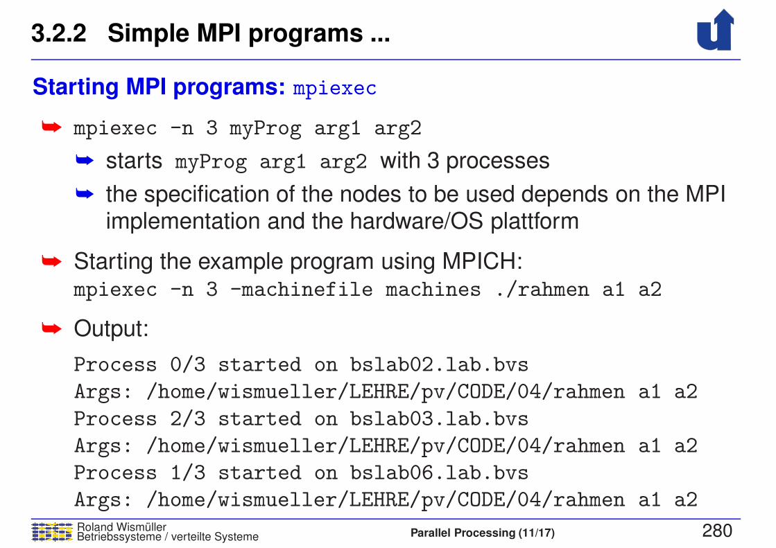
3.2.2 Simple MPI programs ...
Roland WismullerBetriebssysteme / verteilte Systeme Parallel Processing (11/17) 280
Starting MPI programs: mpiexec
➥ mpiexec -n 3 myProg arg1 arg2
➥ starts myProg arg1 arg2 with 3 processes
➥ the specification of the nodes to be used depends on the MPIimplementation and the hardware/OS plattform
➥ Starting the example program using MPICH:mpiexec -n 3 -machinefile machines ./rahmen a1 a2
➥ Output:
Process 0/3 started on bslab02.lab.bvs
Args: /home/wismueller/LEHRE/pv/CODE/04/rahmen a1 a2
Process 2/3 started on bslab03.lab.bvs
Args: /home/wismueller/LEHRE/pv/CODE/04/rahmen a1 a2
Process 1/3 started on bslab06.lab.bvs
Args: /home/wismueller/LEHRE/pv/CODE/04/rahmen a1 a2
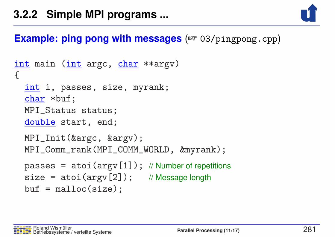
3.2.2 Simple MPI programs ...
Roland WismullerBetriebssysteme / verteilte Systeme Parallel Processing (11/17) 281
Example: ping pong with messages (☞ 03/pingpong.cpp)
int main (int argc, char **argv)
{
int i, passes, size, myrank;
char *buf;
MPI_Status status;
double start, end;
MPI_Init(&argc, &argv);
MPI_Comm_rank(MPI_COMM_WORLD, &myrank);
passes = atoi(argv[1]); // Number of repetitions
size = atoi(argv[2]); // Message length
buf = malloc(size);
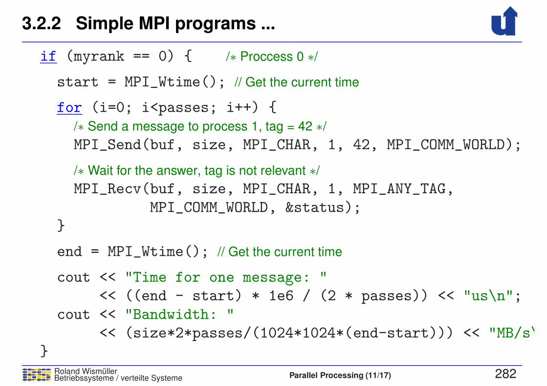
3.2.2 Simple MPI programs ...
Roland WismullerBetriebssysteme / verteilte Systeme Parallel Processing (11/17) 282
if (myrank == 0) { /∗ Proccess 0 ∗/
start = MPI_Wtime(); // Get the current time
for (i=0; i<passes; i++) {/∗ Send a message to process 1, tag = 42 ∗/
MPI_Send(buf, size, MPI_CHAR, 1, 42, MPI_COMM_WORLD);
/∗ Wait for the answer, tag is not relevant ∗/
MPI_Recv(buf, size, MPI_CHAR, 1, MPI_ANY_TAG,
MPI_COMM_WORLD, &status);}
end = MPI_Wtime(); // Get the current time
cout << "Time for one message: "<< ((end - start) * 1e6 / (2 * passes)) << "us\n";
cout << "Bandwidth: "<< (size*2*passes/(1024*1024*(end-start))) << "MB/s\
}
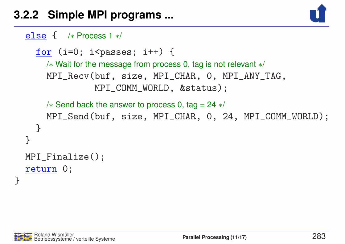
3.2.2 Simple MPI programs ...
Roland WismullerBetriebssysteme / verteilte Systeme Parallel Processing (11/17) 283
else { /∗ Process 1 ∗/
for (i=0; i<passes; i++) {
/∗ Wait for the message from process 0, tag is not relevant ∗/
MPI_Recv(buf, size, MPI_CHAR, 0, MPI_ANY_TAG,
MPI_COMM_WORLD, &status);
/∗ Send back the answer to process 0, tag = 24 ∗/
MPI_Send(buf, size, MPI_CHAR, 0, 24, MPI_COMM_WORLD);
}
}
MPI_Finalize();
return 0;
}
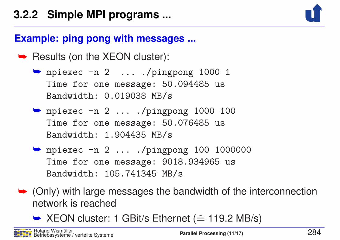
3.2.2 Simple MPI programs ...
Roland WismullerBetriebssysteme / verteilte Systeme Parallel Processing (11/17) 284
Example: ping pong with messages ...
➥ Results (on the XEON cluster):
➥ mpiexec -n 2 ... ./pingpong 1000 1
Time for one message: 50.094485 us
Bandwidth: 0.019038 MB/s
➥ mpiexec -n 2 ... ./pingpong 1000 100
Time for one message: 50.076485 us
Bandwidth: 1.904435 MB/s
➥ mpiexec -n 2 ... ./pingpong 100 1000000
Time for one message: 9018.934965 us
Bandwidth: 105.741345 MB/s
➥ (Only) with large messages the bandwidth of the interconnection
network is reached
➥ XEON cluster: 1 GBit/s Ethernet (= 119.2 MB/s)
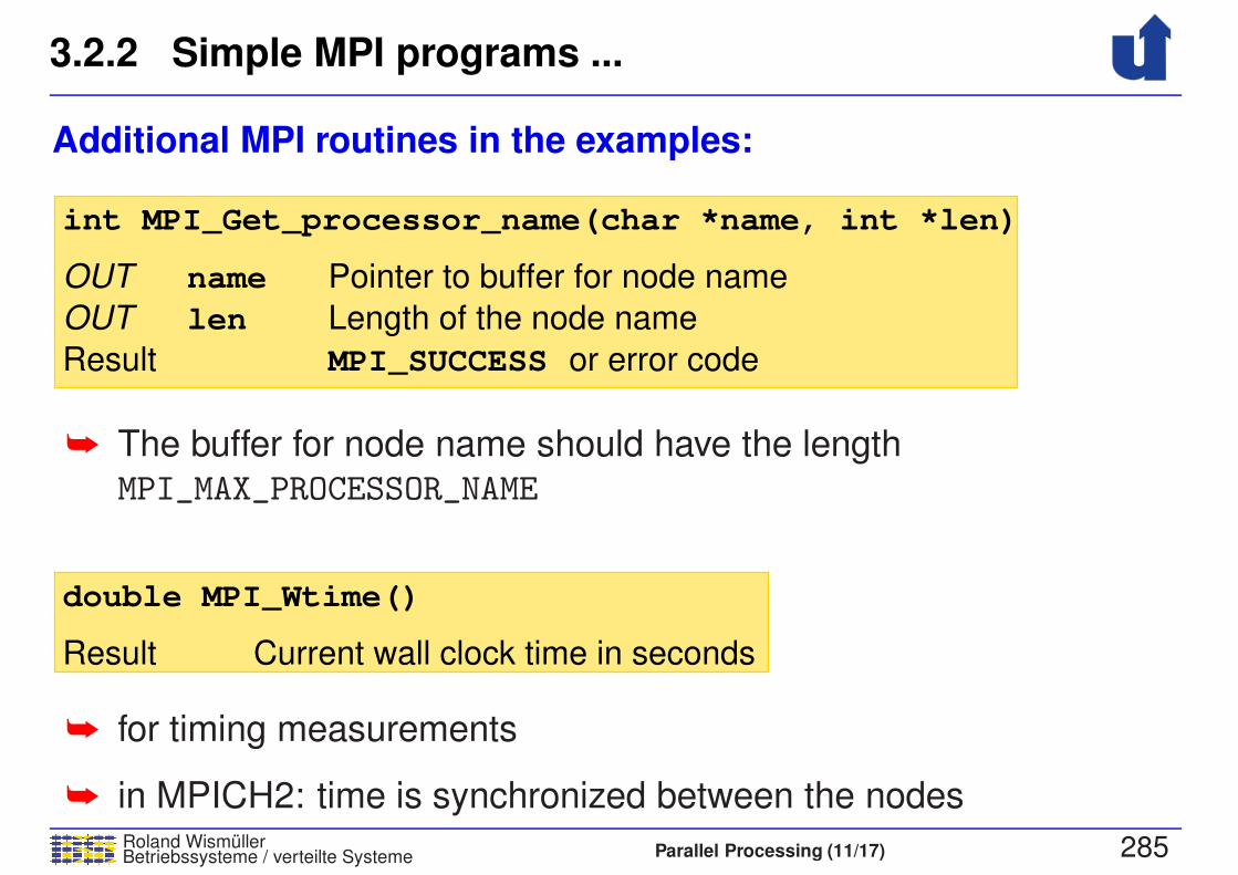
3.2.2 Simple MPI programs ...
Roland WismullerBetriebssysteme / verteilte Systeme Parallel Processing (11/17) 285
Additional MPI routines in the examples:
OUT
OUT
Result
int MPI_Get_processor_name(char *name, int *len)
name
len
MPI_SUCCESS or error code
Pointer to buffer for node name
Length of the node name
➥ The buffer for node name should have the lengthMPI_MAX_PROCESSOR_NAME
double MPI_Wtime()
Result Current wall clock time in seconds
➥ for timing measurements
➥ in MPICH2: time is synchronized between the nodes
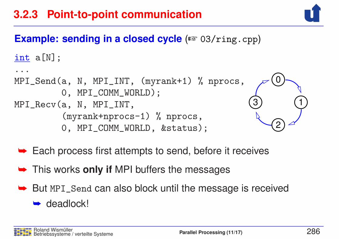
3.2.3 Point-to-point communication
Roland WismullerBetriebssysteme / verteilte Systeme Parallel Processing (11/17) 286
Example: sending in a closed cycle (☞ 03/ring.cpp)
int a[N];
...
MPI_Send(a, N, MPI_INT, (myrank+1) % nprocs,
0, MPI_COMM_WORLD);
MPI_Recv(a, N, MPI_INT,
(myrank+nprocs-1) % nprocs,
0, MPI_COMM_WORLD, &status);
13
2
0
➥ Each process first attempts to send, before it receives
➥ This works only if MPI buffers the messages
➥ But MPI_Send can also block until the message is received
➥ deadlock!
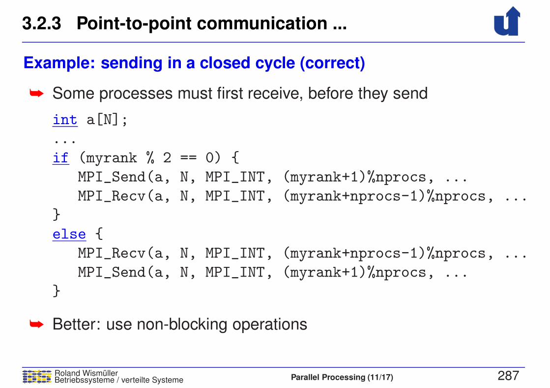
3.2.3 Point-to-point communication ...
Roland WismullerBetriebssysteme / verteilte Systeme Parallel Processing (11/17) 287
Example: sending in a closed cycle (correct)
➥ Some processes must first receive, before they send
int a[N];
...
if (myrank % 2 == 0) {
MPI_Send(a, N, MPI_INT, (myrank+1)%nprocs, ...
MPI_Recv(a, N, MPI_INT, (myrank+nprocs-1)%nprocs, ...
}
else {
MPI_Recv(a, N, MPI_INT, (myrank+nprocs-1)%nprocs, ...
MPI_Send(a, N, MPI_INT, (myrank+1)%nprocs, ...
}
➥ Better: use non-blocking operations
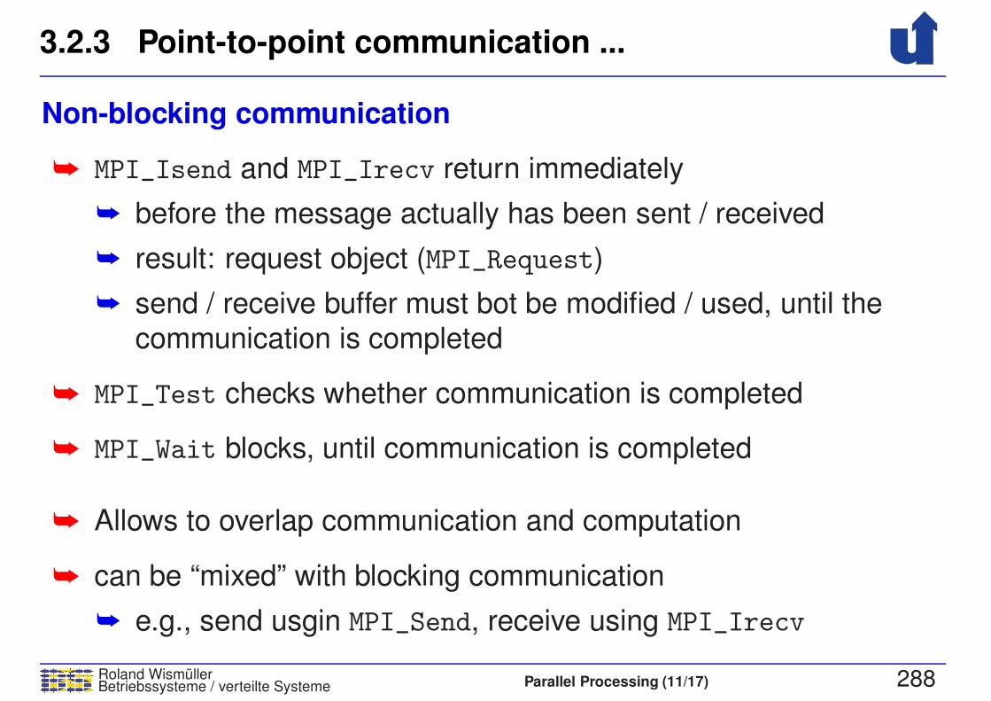
3.2.3 Point-to-point communication ...
Roland WismullerBetriebssysteme / verteilte Systeme Parallel Processing (11/17) 288
Non-blocking communication
➥ MPI_Isend and MPI_Irecv return immediately
➥ before the message actually has been sent / received
➥ result: request object (MPI_Request)
➥ send / receive buffer must bot be modified / used, until the
communication is completed
➥ MPI_Test checks whether communication is completed
➥ MPI_Wait blocks, until communication is completed
➥ Allows to overlap communication and computation
➥ can be “mixed” with blocking communication
➥ e.g., send usgin MPI_Send, receive using MPI_Irecv
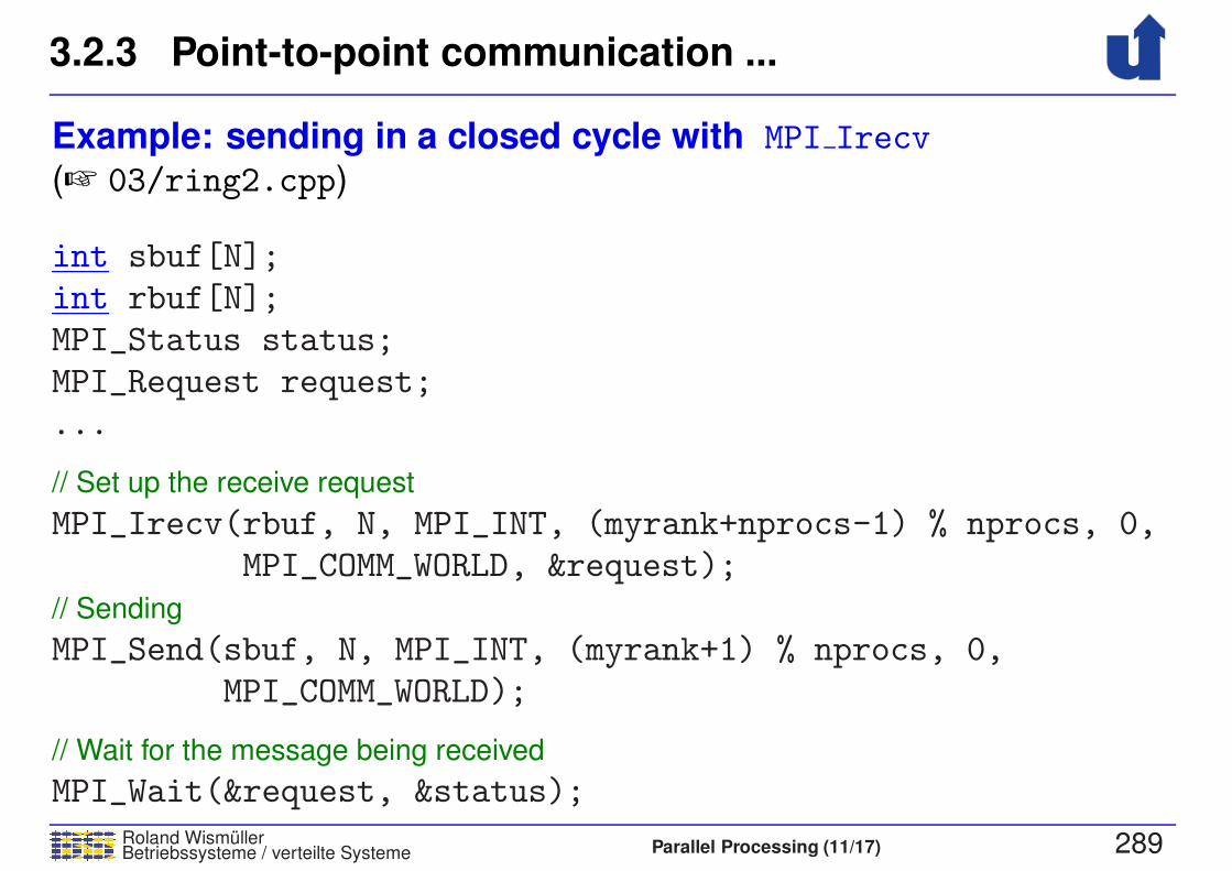
3.2.3 Point-to-point communication ...
Roland WismullerBetriebssysteme / verteilte Systeme Parallel Processing (11/17) 289
Example: sending in a closed cycle with MPI Irecv
(☞ 03/ring2.cpp)
int sbuf[N];int rbuf[N];MPI_Status status;MPI_Request request;
...
// Set up the receive request
MPI_Irecv(rbuf, N, MPI_INT, (myrank+nprocs-1) % nprocs, 0,MPI_COMM_WORLD, &request);
// Sending
MPI_Send(sbuf, N, MPI_INT, (myrank+1) % nprocs, 0,MPI_COMM_WORLD);
// Wait for the message being received
MPI_Wait(&request, &status);
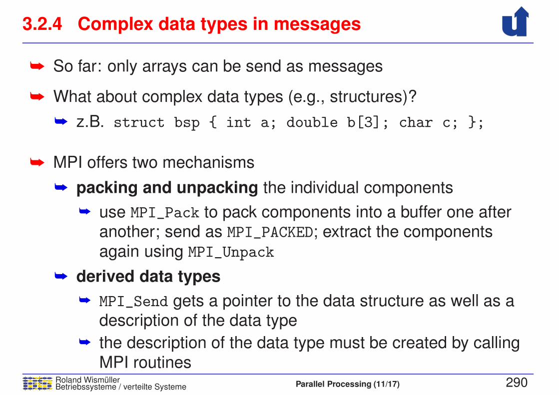
3.2.4 Complex data types in messages
Roland WismullerBetriebssysteme / verteilte Systeme Parallel Processing (11/17) 290
➥ So far: only arrays can be send as messages
➥ What about complex data types (e.g., structures)?
➥ z.B. struct bsp { int a; double b[3]; char c; };
➥ MPI offers two mechanisms
➥ packing and unpacking the individual components
➥ use MPI_Pack to pack components into a buffer one afteranother; send as MPI_PACKED; extract the components
again using MPI_Unpack
➥ derived data types
➥ MPI_Send gets a pointer to the data structure as well as adescription of the data type
➥ the description of the data type must be created by calling
MPI routines

3.2.4 Complex data types in messages ...
Roland WismullerBetriebssysteme / verteilte Systeme Parallel Processing (11/17) 291
Derived data types
➥ MPI offers constructors, which can be used to define own
(derived) data types:
➥ for contiguous data: MPI Type contiguous
➥ allows the definition of array types
➥ for non-contiguous data: MPI Type vector
➥ e.g., for a column of a matrix or a sub-matrix
➥ for structures: MPI Type create struct
➥ After a new data type has been created, it must be “announced”:
MPI Type commit
➥ After that, the data type can be used like a predefined data type
(e.g., MPI INT)
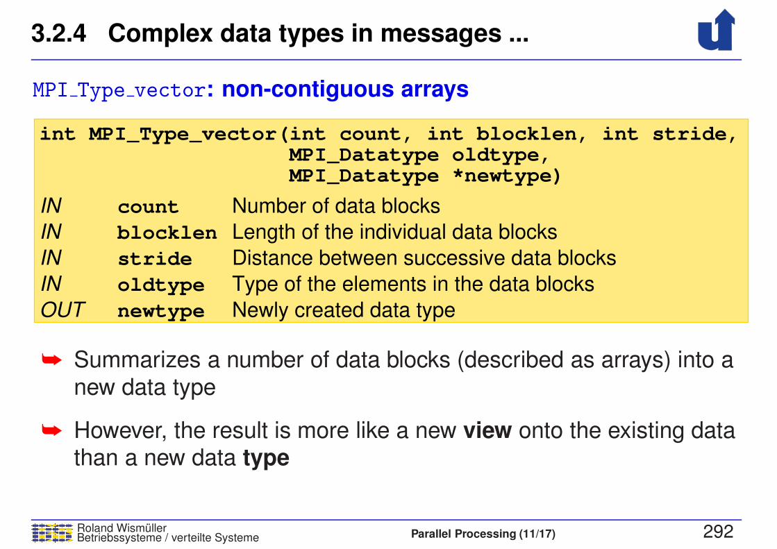
3.2.4 Complex data types in messages ...
Roland WismullerBetriebssysteme / verteilte Systeme Parallel Processing (11/17) 292
MPI Type vector: non-contiguous arrays
IN
OUT
oldtype
newtype Newly created data type
Type of the elements in the data blocks
int MPI_Type_vector(int count, int blocklen, int stride,MPI_Datatype oldtype,MPI_Datatype *newtype)
IN count
IN blocklen
Number of data blocks
IN stride
Length of the individual data blocks
Distance between successive data blocks
➥ Summarizes a number of data blocks (described as arrays) into a
new data type
➥ However, the result is more like a new view onto the existing datathan a new data type
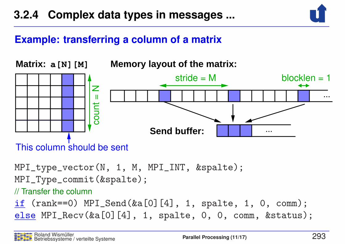
3.2.4 Complex data types in messages ...
Roland WismullerBetriebssysteme / verteilte Systeme Parallel Processing (11/17) 293
Example: transferring a column of a matrix
...
Memory layout of the matrix:Matrix:
blocklen = 1
a[N][M]
stride = M
count =
N
This column should be sent
Send buffer: ...
MPI_type_vector(N, 1, M, MPI_INT, &spalte);
MPI_Type_commit(&spalte);
// Transfer the column
if (rank==0) MPI_Send(&a[0][4], 1, spalte, 1, 0, comm);
else MPI_Recv(&a[0][4], 1, spalte, 0, 0, comm, &status);
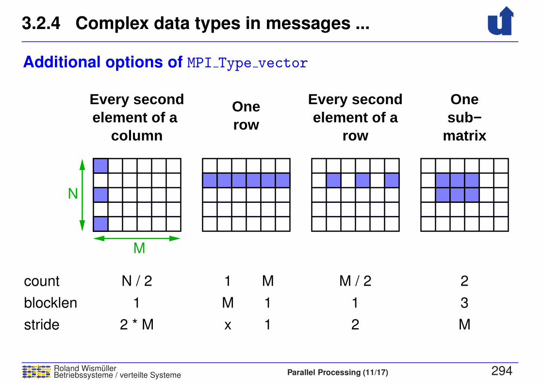
3.2.4 Complex data types in messages ...
Roland WismullerBetriebssysteme / verteilte Systeme Parallel Processing (11/17) 294
Additional options of MPI Type vector
count
blocklen
stride
1
2 * M
1
M
1
1
M
x 2 M
3
2N / 2 M / 2
1
column
Every secondelement of a row
One Every secondelement of a
row
Onesub−
matrix
N
M
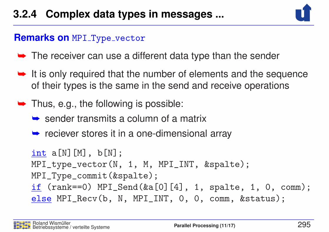
3.2.4 Complex data types in messages ...
Roland WismullerBetriebssysteme / verteilte Systeme Parallel Processing (11/17) 295
Remarks on MPI Type vector
➥ The receiver can use a different data type than the sender
➥ It is only required that the number of elements and the sequence
of their types is the same in the send and receive operations
➥ Thus, e.g., the following is possible:
➥ sender transmits a column of a matrix
➥ reciever stores it in a one-dimensional array
int a[N][M], b[N];
MPI_type_vector(N, 1, M, MPI_INT, &spalte);
MPI_Type_commit(&spalte);
if (rank==0) MPI_Send(&a[0][4], 1, spalte, 1, 0, comm);
else MPI_Recv(b, N, MPI_INT, 0, 0, comm, &status);
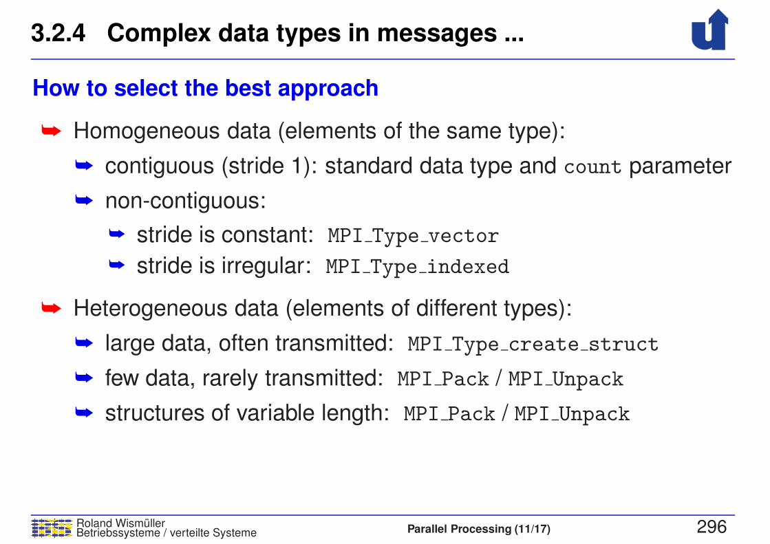
3.2.4 Complex data types in messages ...
Roland WismullerBetriebssysteme / verteilte Systeme Parallel Processing (11/17) 296
How to select the best approach
➥ Homogeneous data (elements of the same type):
➥ contiguous (stride 1): standard data type and count parameter
➥ non-contiguous:
➥ stride is constant: MPI Type vector
➥ stride is irregular: MPI Type indexed
➥ Heterogeneous data (elements of different types):
➥ large data, often transmitted: MPI Type create struct
➥ few data, rarely transmitted: MPI Pack / MPI Unpack
➥ structures of variable length: MPI Pack / MPI Unpack
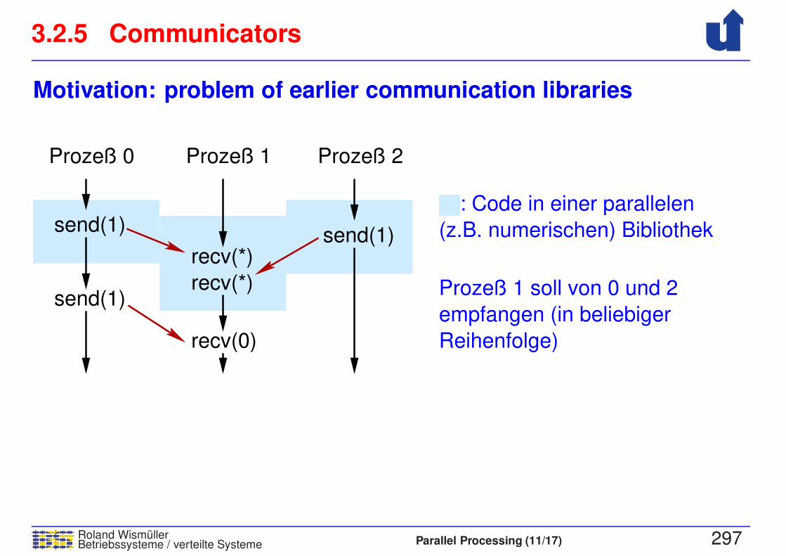
3.2.5 Communicators
Roland WismullerBetriebssysteme / verteilte Systeme Parallel Processing (11/17) 297
Motivation: problem of earlier communication libraries
: Code in einer parallelen
(z.B. numerischen) Bibliothek
Prozeß 1 Prozeß 2Prozeß 0
recv(*)
send(1)
send(1)
Prozeß 1 soll von 0 und 2
empfangen (in beliebiger
Reihenfolge)
recv(*)
send(1)
recv(0)
➥ Message tags are not a reliable solution
➥ tags might be chosen identically by chance!
➥ Required: different communication contexts

3.2.5 Communicators
Roland WismullerBetriebssysteme / verteilte Systeme Parallel Processing (11/17) 297
Motivation: problem of earlier communication libraries
: Code in einer parallelen
(z.B. numerischen) Bibliothek
Prozeß 1 Prozeß 2Prozeß 0
recv(*)
send(1)
send(1)
Falls Prozeß 2 aus irgendeinem Grund "verspätet" ist:Kommunikation schlägt fehl!
send(1)recv(*)
➥ Message tags are not a reliable solution
➥ tags might be chosen identically by chance!
➥ Required: different communication contexts
3.2.5 Communicators ...
Roland WismullerBetriebssysteme / verteilte Systeme Parallel Processing (11/17) 298
➥ Communicator = process group + context
➥ Communicators support
➥ working with process groups
➥ task parallelism
➥ coupled simulations
➥ collective communication with a subset of all processes
➥ communication contexts
➥ for parallel libraries
➥ A communicator represents a communication domain
➥ communication is possible only within the same domain
➥ no wild-card for communicator in MPI_Recv
➥ a process can belong to several domains at the same time
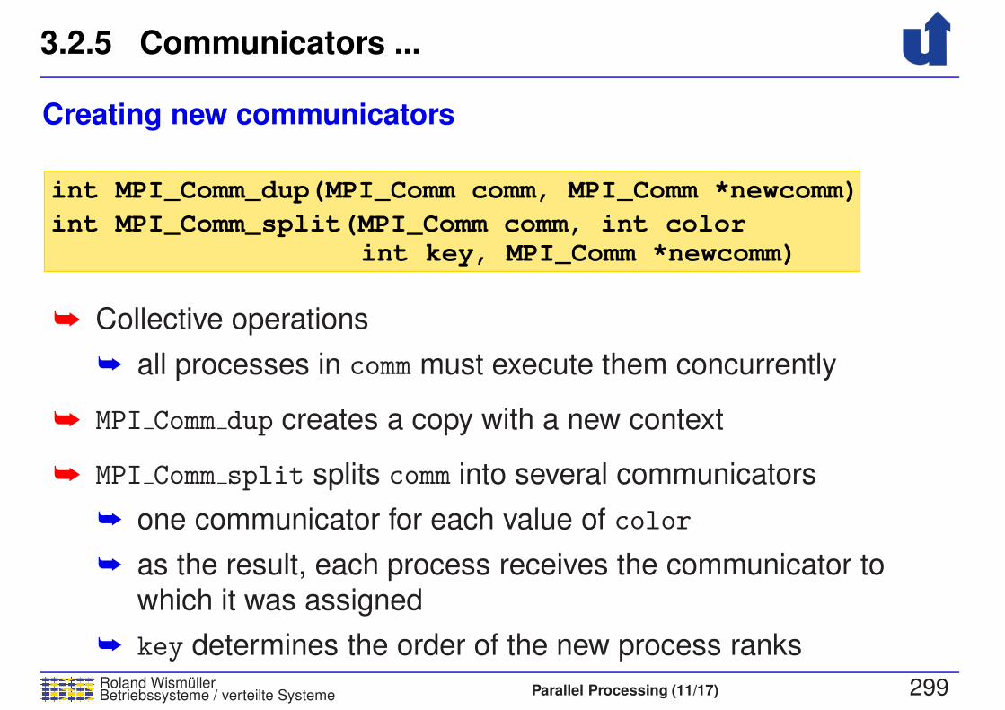
3.2.5 Communicators ...
Roland WismullerBetriebssysteme / verteilte Systeme Parallel Processing (11/17) 299
Creating new communicators
int MPI_Comm_split(MPI_Comm comm, int colorint key, MPI_Comm *newcomm)
int MPI_Comm_dup(MPI_Comm comm, MPI_Comm *newcomm)
➥ Collective operations
➥ all processes in comm must execute them concurrently
➥ MPI Comm dup creates a copy with a new context
➥ MPI Comm split splits comm into several communicators
➥ one communicator for each value of color
➥ as the result, each process receives the communicator to
which it was assigned
➥ key determines the order of the new process ranks
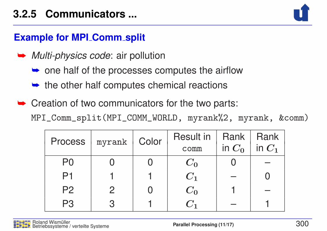
3.2.5 Communicators ...
Roland WismullerBetriebssysteme / verteilte Systeme Parallel Processing (11/17) 300
Example for MPI Comm split
➥ Multi-physics code: air pollution
➥ one half of the processes computes the airflow
➥ the other half computes chemical reactions
➥ Creation of two communicators for the two parts:
MPI_Comm_split(MPI_COMM_WORLD, myrank%2, myrank, &comm)
Result in Rank RankProcess myrank Color
comm in C0 in C1
P0 0 0 C0 0 –
P1 1 1 C1 – 0
P2 2 0 C0 1 –
P3 3 1 C1 – 1

3.2.6 Collective operations
Roland WismullerBetriebssysteme / verteilte Systeme Parallel Processing (11/17) 301
➥ Collective operations in MPI
➥ must be executed concurrently by all processes of a process
group (a communicator)
➥ are blocking
➥ do not neccessarily result in a global (barrier) synchronisation,
however
➥ Collective synchronisation and communication functions
➥ barriers
➥ communication: broadcast, scatter, gather, ...
➥ reductions (communication with aggregation)
3.2.6 Collective operations ...
Roland WismullerBetriebssysteme / verteilte Systeme Parallel Processing (11/17) 302
MPI Barrier
int MPI_Barrier(MPI_Comm comm)
➥ Barrier synchonization of all processes in comm
➥ With message passing, barriers are actually not really necessary
➥ synchonization is achieved by message exchange
➥ Reasons for barriers:
➥ more easy understanding of the program
➥ timing measurements, debugging output
➥ input/output?? (console, file)
➥ some very special situations in MPI (see the standard ...)

Roland WismullerBetriebssysteme / verteilte Systeme Parallel Processing (12/17) xiii
Roland Wismuller
Universitat Siegen
Tel.: 0271/740-4050, Buro: H-B 8404
Stand: January 23, 2018
Parallel Processing
WS 2017/18
08.01.2018
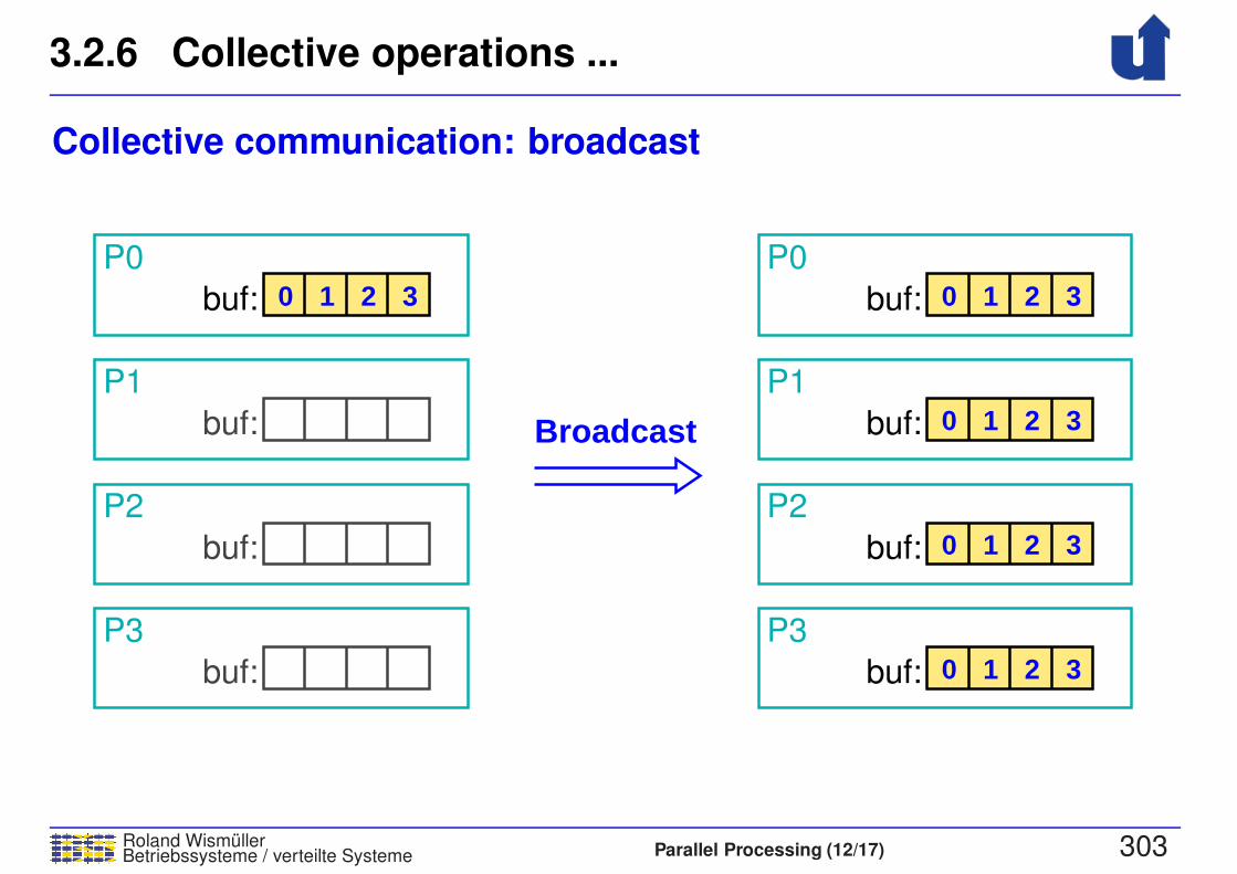
3.2.6 Collective operations ...
Roland WismullerBetriebssysteme / verteilte Systeme Parallel Processing (12/17) 303
Collective communication: broadcast
0 1 2 3 0 1 2 3
0 1 2 3
0 1 2 3
0 1 2 3buf:
buf:
buf: Broadcast
P3
P2
buf:
P0
buf:
P1
buf:
P2
buf:
P3
buf:
P0
P1
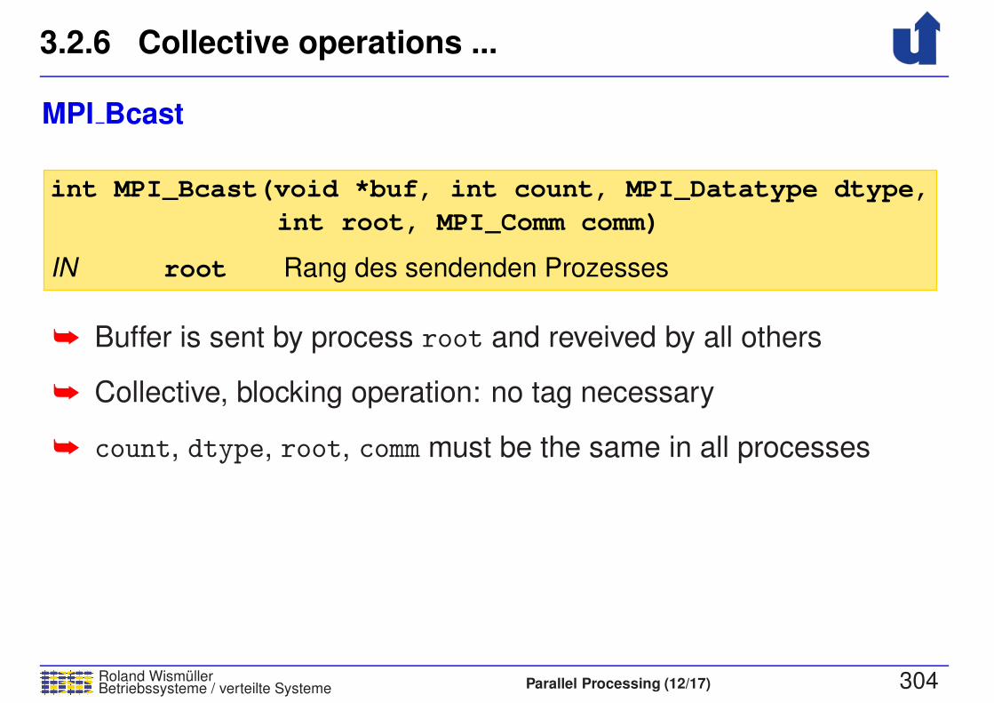
3.2.6 Collective operations ...
Roland WismullerBetriebssysteme / verteilte Systeme Parallel Processing (12/17) 304
MPI Bcast
IN root Rang des sendenden Prozesses
int MPI_Bcast(void *buf, int count, MPI_Datatype dtype,
int root, MPI_Comm comm)
➥ Buffer is sent by process root and reveived by all others
➥ Collective, blocking operation: no tag necessary
➥ count, dtype, root, comm must be the same in all processes
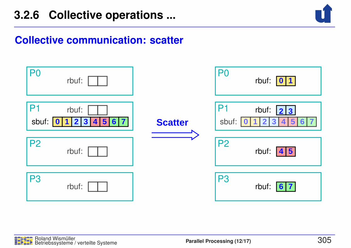
3.2.6 Collective operations ...
Roland WismullerBetriebssysteme / verteilte Systeme Parallel Processing (12/17) 305
Collective communication: scatter
rbuf:
rbuf:
rbuf:
rbuf: rbuf:
rbuf:
rbuf:
rbuf:
P3
P2
P1
P0 P0
P1
P2
P3
0 1
2 3
4 5
6 7
Scatter 0 1 2 3 4 5 6 70 1 2 3 4 5 6 7 sbuf:sbuf:

3.2.6 Collective operations ...
Roland WismullerBetriebssysteme / verteilte Systeme Parallel Processing (12/17) 306
MPI Scatter
int MPI_Scatter(void *sendbuf, int sendcount,
void *recvbuf, int recvcount,
MPI_Datatype sendtype,
MPI_Datatype recvtype,
int root, MPI_Comm comm)
➥ Process root sends a part of the data to each process
➥ including itself
➥ sendcount: data length for each process (not the total length!)
➥ Process i receives sendcount elements of sendbuf starting fromposition i * sendcount
➥ Alternative MPI_Scatterv: length and position can be specifiedindividually for each receiver
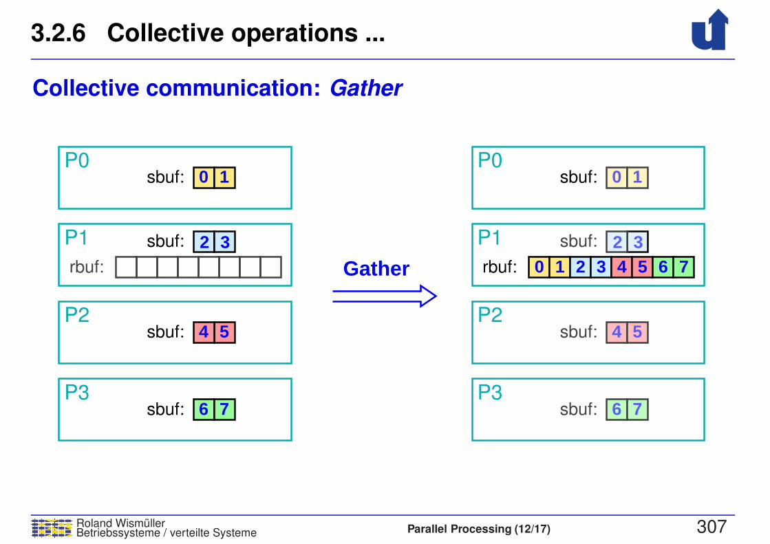
3.2.6 Collective operations ...
Roland WismullerBetriebssysteme / verteilte Systeme Parallel Processing (12/17) 307
Collective communication: Gather
sbuf:
sbuf:
sbuf:
sbuf: sbuf:
sbuf:
sbuf:
sbuf:
Gather
P0
P1
P2
P3 P3
P2
P1
P0
0 1 2 3 4 5 6 7
0 1
4 5
6 7
0 1
32 2 3
4 5
6 7
rbuf:rbuf:
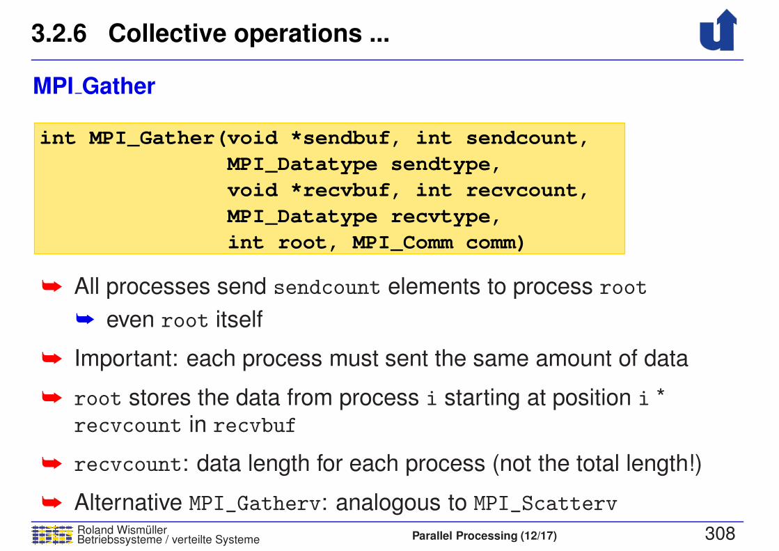
3.2.6 Collective operations ...
Roland WismullerBetriebssysteme / verteilte Systeme Parallel Processing (12/17) 308
MPI Gather
void *recvbuf, int recvcount,
MPI_Datatype sendtype,
MPI_Datatype recvtype,
int root, MPI_Comm comm)
int MPI_Gather(void *sendbuf, int sendcount,
➥ All processes send sendcount elements to process root
➥ even root itself
➥ Important: each process must sent the same amount of data
➥ root stores the data from process i starting at position i *recvcount in recvbuf
➥ recvcount: data length for each process (not the total length!)
➥ Alternative MPI_Gatherv: analogous to MPI_Scatterv
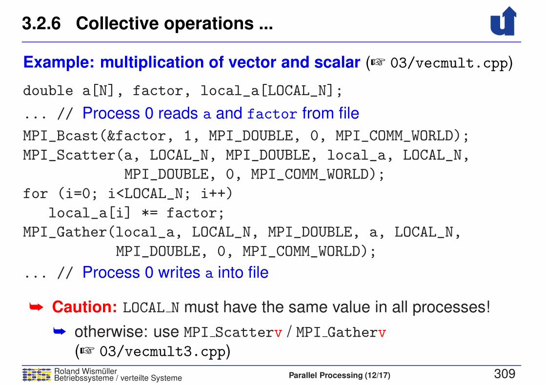
3.2.6 Collective operations ...
Roland WismullerBetriebssysteme / verteilte Systeme Parallel Processing (12/17) 309
Example: multiplication of vector and scalar (☞ 03/vecmult.cpp)
double a[N], factor, local_a[LOCAL_N];
... // Process 0 reads a and factor from file
MPI_Bcast(&factor, 1, MPI_DOUBLE, 0, MPI_COMM_WORLD);
MPI_Scatter(a, LOCAL_N, MPI_DOUBLE, local_a, LOCAL_N,
MPI_DOUBLE, 0, MPI_COMM_WORLD);
for (i=0; i<LOCAL_N; i++)
local_a[i] *= factor;
MPI_Gather(local_a, LOCAL_N, MPI_DOUBLE, a, LOCAL_N,
MPI_DOUBLE, 0, MPI_COMM_WORLD);
... // Process 0 writes a into file
➥ Caution: LOCAL N must have the same value in all processes!
➥ otherwise: use MPI Scatterv / MPI Gatherv
(☞ 03/vecmult3.cpp)
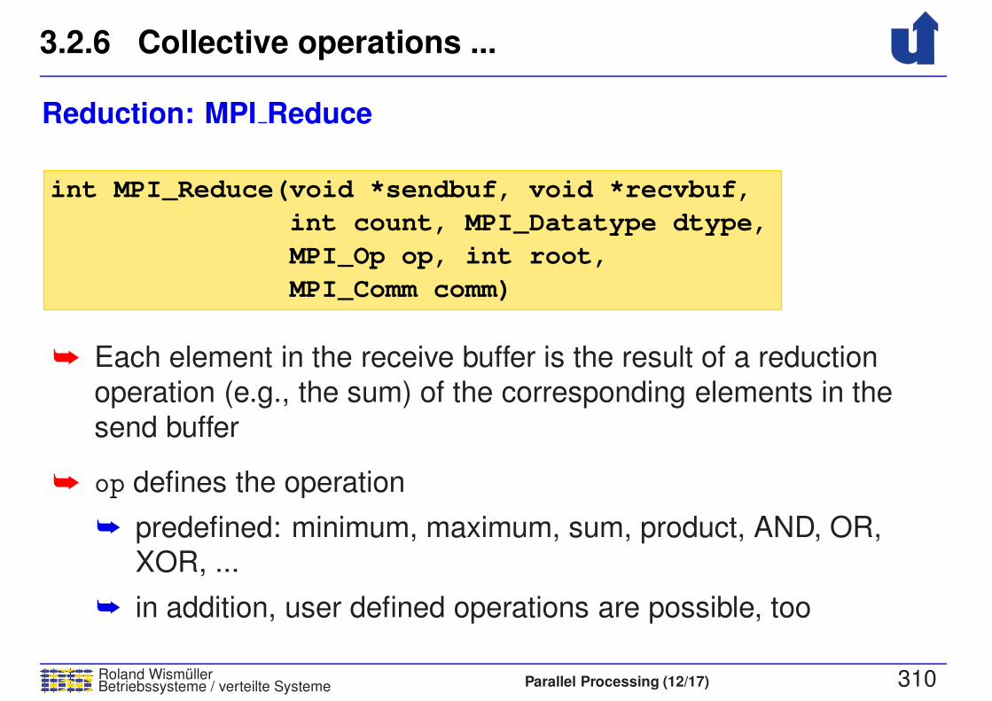
3.2.6 Collective operations ...
Roland WismullerBetriebssysteme / verteilte Systeme Parallel Processing (12/17) 310
Reduction: MPI Reduce
int MPI_Reduce(void *sendbuf, void *recvbuf,
int count, MPI_Datatype dtype,
MPI_Op op, int root,
MPI_Comm comm)
➥ Each element in the receive buffer is the result of a reduction
operation (e.g., the sum) of the corresponding elements in the
send buffer
➥ op defines the operation
➥ predefined: minimum, maximum, sum, product, AND, OR,XOR, ...
➥ in addition, user defined operations are possible, too
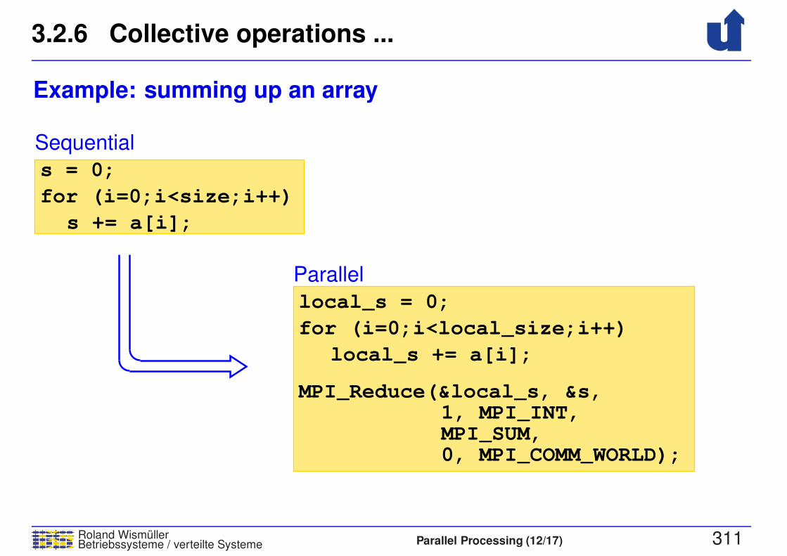
3.2.6 Collective operations ...
Roland WismullerBetriebssysteme / verteilte Systeme Parallel Processing (12/17) 311
Example: summing up an array
for (i=0;i<size;i++)
Sequential
for (i=0;i<local_size;i++)
s += a[i];
s = 0;
local_s = 0;
local_s += a[i];
Parallel
1, MPI_INT,MPI_SUM,0, MPI_COMM_WORLD);
MPI_Reduce(&local_s, &s,

3.2.6 Collective operations ...
Roland WismullerBetriebssysteme / verteilte Systeme Parallel Processing (12/17) 312
More collective communication operations
➥ MPI_Alltoall: all-to-all broadcast (☞ 1.9.5)
➥ MPI_Allgather and MPI_Allgatherv: at the end, all processes
have the gathered data
➥ corresponds to a gather with subsequent broadcast
➥ MPI_Allreduce: at the end, all processes have the result of the
reduction
➥ corresponds to a reduce with subsequent broadcast
➥ MPI_Scan: prefix reduction
➥ e.g., using the sum: process i receives the sum of the data
from processes 0 up to and including i
3.2.7 Further concepts
Roland WismullerBetriebssysteme / verteilte Systeme Parallel Processing (12/17) 313
➥ Topologies
➥ the application’s communication structure is stored in acommunicator➥ e.g., cartesian grid
➥ allows to simplify and optimize the communication
➥ e,g,. “send to the left neighbor”
➥ the communicating processes can be placed onneighboring nodes
➥ Dynamic process creation (since MPI-2)
➥ new processes can be created at run-time
➥ process creation is a collective operation
➥ the newly created process group gets its own MPI COMM WORLD
➥ communication between process groups uses anintercommunicator
3.2.7 Further concepts ...
Roland WismullerBetriebssysteme / verteilte Systeme Parallel Processing (12/17) 314
➥ One-sided communication (since MPI-2)
➥ access to the address space of other processes
➥ operations: read, write, atomic update
➥ weak consistency model
➥ explicit fence and lock /unlock operations for
synchronisation
➥ useful for applications with irregular communication
➥ one process alone can execute the communication
➥ Parallel I/O (since MPI-2)
➥ processes have individual views to a file
➥ specifiec by an MPI data type
➥ file operations: individual / collective, private / shared file
pointer, blocking / non-blocking
3.2.8 Summary
Roland WismullerBetriebssysteme / verteilte Systeme Parallel Processing (12/17) 315
➥ Basic routines:
➥ Init, Finalize, Comm_size, Comm_rank, Send, Recv
➥ Complex data types in messages
➥ Pack and Unpack
➥ user defined data types
➥ also for non-contiguous data
(e.g., column of a matrix)
➥ Communicators: process group + communication context
➥ Non-blocking communication: Isend, Irecv, Test, Wait
➥ Collective operations
➥ Barrier, Bcast, Scatter(v), Gather(v), Reduce, ...

Roland WismullerBetriebssysteme / verteilte Systeme Parallel Processing (12/17) 316
Parallel ProcessingWS 2017/18
4 Optimization Techniques
4 Optimization Techniques ...
Roland WismullerBetriebssysteme / verteilte Systeme Parallel Processing (12/17) 317
➥ In the following: examples for important techniques to optimize
parallel programs
➥ Shared memory:
➥ cache optimization: improve the locality of memory accesses
➥ loop interchange, tiling
➥ array padding
➥ false sharing
➥ Message passing:
➥ combining messages
➥ latency hiding
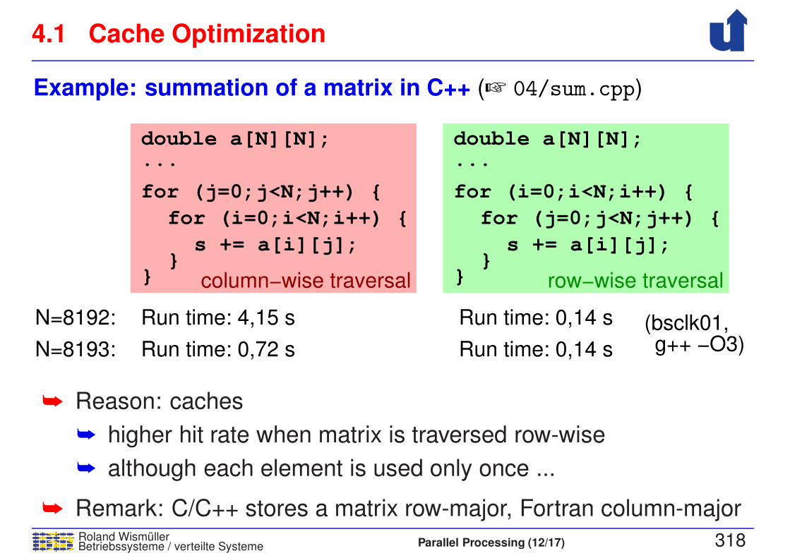
4.1 Cache Optimization
Roland WismullerBetriebssysteme / verteilte Systeme Parallel Processing (12/17) 318
Example: summation of a matrix in C++ (☞ 04/sum.cpp)
N=8192:
N=8193:
Run time: 4,15 s Run time: 0,14 s
Run time: 0,72 s Run time: 0,14 s
double a[N][N];...
s += a[i][j];}
}
double a[N][N];...
for (j=0;j<N;j++) {
for (i=0;i<N;i++) {
s += a[i][j];}
}
for (i=0;i<N;i++) {
for (j=0;j<N;j++) {
row−wise traversalcolumn−wise traversal
(bsclk01,g++ −O3)
➥ Reason: caches
➥ higher hit rate when matrix is traversed row-wise
➥ although each element is used only once ...
➥ Remark: C/C++ stores a matrix row-major, Fortran column-major

4.1 Cache Optimization ...
Roland WismullerBetriebssysteme / verteilte Systeme Parallel Processing (12/17) 319
Details on caches: cache lines
➥ Storage of data in the cache and transfer between main memory
and cache are performed using larger blocks
➥ reason: after a memory cell has been addressed, the
subsequent cells can be read very fast
➥ size of a cache line: 32-128 Byte
➥ In the example:
➥ row-wise traversal: after the cache line for a[i][j] has been
loaded, the values of a[i+1][j], a[i+2][j], ... are already in
the cache, too
➥ column-wise traversal: the cache line for a[i][j] has already
been evicted, when a[i+1][j], ... are used
➥ Rule: traverse memory in linearly increasing order, if possible!

4.1 Cache Optimization ...
Roland WismullerBetriebssysteme / verteilte Systeme Parallel Processing (12/17) 320
Details on caches: set-associative caches
➥ A memory block (with given address) can be stored only at a few
places in the cache
➥ reason: easy retrieval of the data in hardware
➥ usually, a set has 2 to 8 entries
➥ the entry within a set is determined using the LRU strategy
➥ The lower k Bits of the address determine the set
(k depends on cache size and degree of associativity)
➥ for all memory locations, whose lower k address bits are the
same, there are only 2 - 8 possible cache entries!

4.1 Cache Optimization ...
Roland WismullerBetriebssysteme / verteilte Systeme Parallel Processing (12/17) 321
Details on caches: set-associative caches ...
➥ In the example: with N = 8192 and column-wise traversal
➥ a cache entry is guaranteed to be evicted after a few iterations
of the i-loop (address distance is a power of two)
➥ cache hit rate is very close to zero
➥ Rule: when traversing memory, avoid address distances that are
a power of two!
➥ (avoid powers of two as matrix size for large matrices)
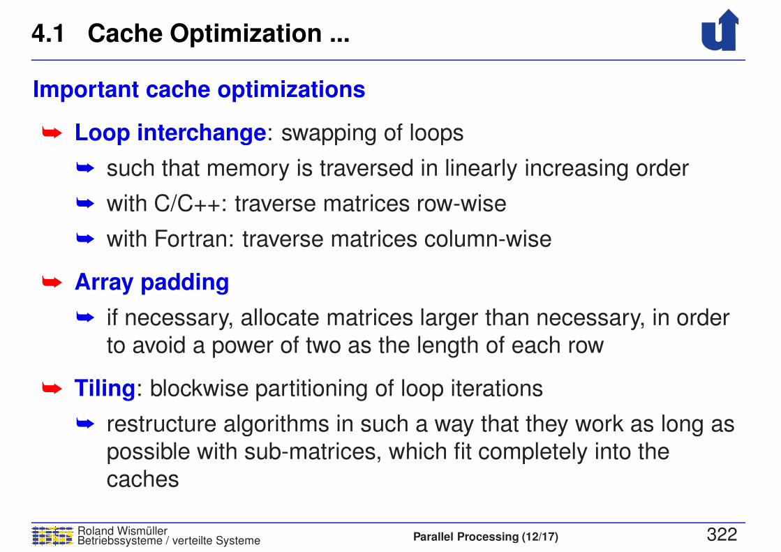
4.1 Cache Optimization ...
Roland WismullerBetriebssysteme / verteilte Systeme Parallel Processing (12/17) 322
Important cache optimizations
➥ Loop interchange: swapping of loops
➥ such that memory is traversed in linearly increasing order
➥ with C/C++: traverse matrices row-wise
➥ with Fortran: traverse matrices column-wise
➥ Array padding
➥ if necessary, allocate matrices larger than necessary, in order
to avoid a power of two as the length of each row
➥ Tiling: blockwise partitioning of loop iterations
➥ restructure algorithms in such a way that they work as long as
possible with sub-matrices, which fit completely into the
caches
Roland WismullerBetriebssysteme / verteilte Systeme Parallel Processing (13/17) xiv
Roland Wismuller
Universitat Siegen
Tel.: 0271/740-4050, Buro: H-B 8404
Stand: January 23, 2018
Parallel Processing
WS 2017/18
15.01.2018

4.1 Cache Optimization ...
Roland WismullerBetriebssysteme / verteilte Systeme Parallel Processing (13/17) 323
(☞ 04/matmult.c)Example: Matrix multiply
➥ Naive code:
for (j=0; j<N; j++)
for (k=0; k<N; k++)
double a[N][N], b[N][N], ...
for (i=0; i<N; i++)
c[i][j] += a[i][k] * b[k][j];
➥ Performance with different compiler optimization levels:
(N=500, g++ 4.6.3, Intel Core i7 2.8 GHz (bspc02))
➥ -O0: 0.3 GFlop/s
➥ -O: 1.3 GFlop/s
➥ -O2: 1.3 GFlop/s
➥ -O3: 2.4 GFlop/s (SIMD vectorization!)
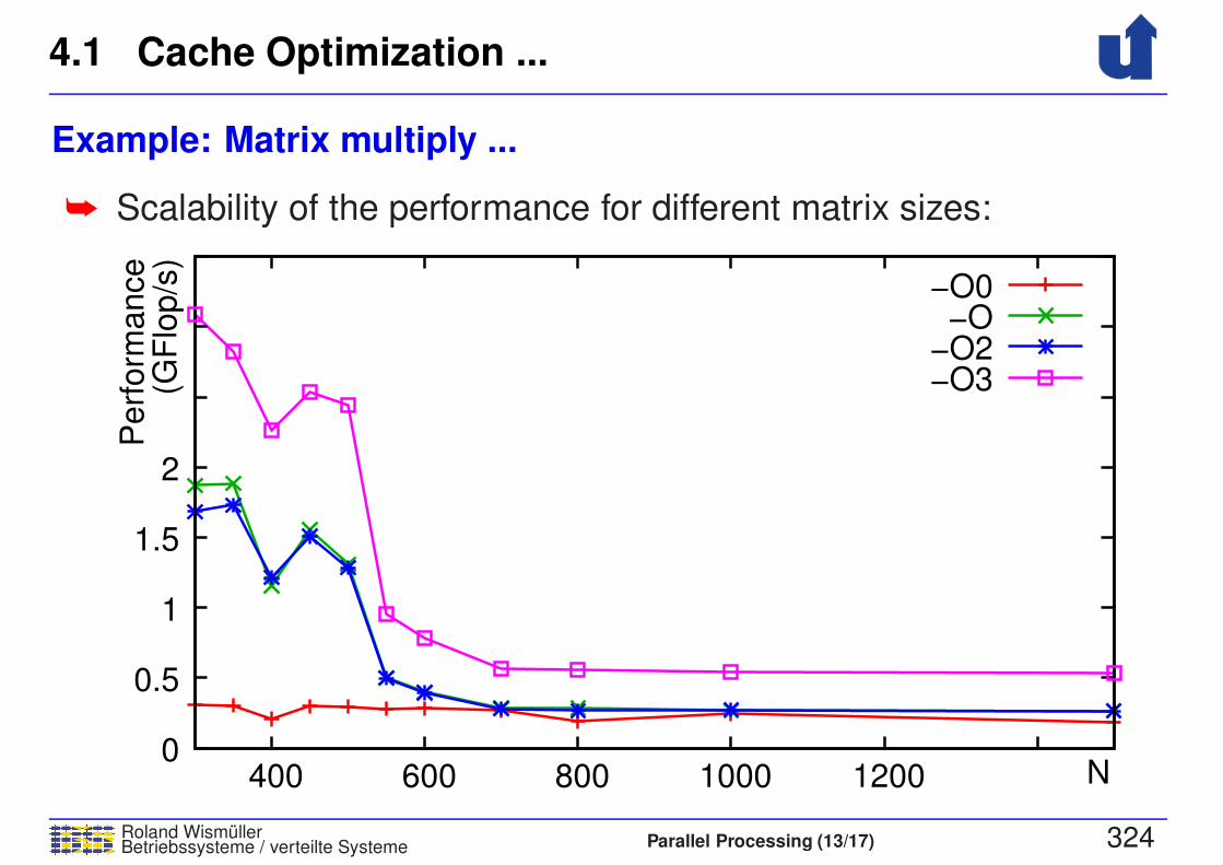
4.1 Cache Optimization ...
Roland WismullerBetriebssysteme / verteilte Systeme Parallel Processing (13/17) 324
Example: Matrix multiply ...
➥ Scalability of the performance for different matrix sizes:
−O0−O
−O2−O3
0
0.5
1
1.5
2
400 600 800 1000 1200 N
Perf
orm
ance
(GF
lop/s
)
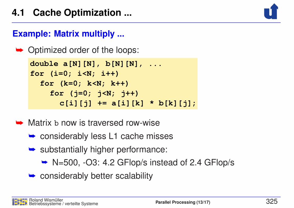
4.1 Cache Optimization ...
Roland WismullerBetriebssysteme / verteilte Systeme Parallel Processing (13/17) 325
Example: Matrix multiply ...
➥ Optimized order of the loops:
double a[N][N], b[N][N], ...
for (i=0; i<N; i++)
c[i][j] += a[i][k] * b[k][j];
for (k=0; k<N; k++)
for (j=0; j<N; j++)
➥ Matrix b now is traversed row-wise
➥ considerably less L1 cache misses
➥ substantially higher performance:
➥ N=500, -O3: 4.2 GFlop/s instead of 2.4 GFlop/s
➥ considerably better scalability

4.1 Cache Optimization ...
Roland WismullerBetriebssysteme / verteilte Systeme Parallel Processing (13/17) 326
Example: Matrix multiply ...
➥ Comparison of both loop orders:
Mis
ses/F
lop
N
0.1
0.2
(GF
lop/s
)P
erf
orm
ance
ijk:GFlop/sijk:L1−Missesijk:L2−Missesijk:L3−Misses
0
1
2
400 600 800 1000 1200
3
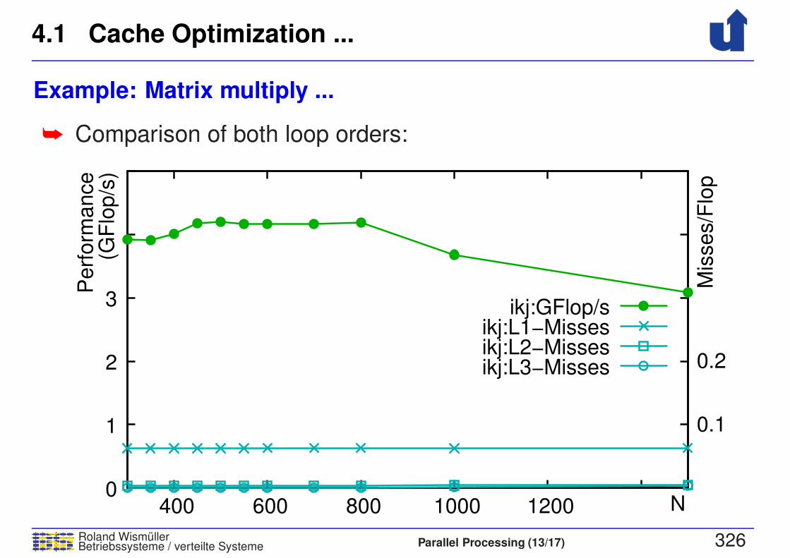
4.1 Cache Optimization ...
Roland WismullerBetriebssysteme / verteilte Systeme Parallel Processing (13/17) 326
Example: Matrix multiply ...
➥ Comparison of both loop orders:
Mis
ses/F
lop
N
0.1
0.2
(GF
lop/s
)P
erf
orm
ance
ikj:GFlop/sikj:L1−Missesikj:L2−Missesikj:L3−Misses
0
1
2
400 600 800 1000 1200
3

Roland WismullerBetriebssysteme / verteilte Systeme Parallel Processing (14/17) xv
Roland Wismuller
Universitat Siegen
Tel.: 0271/740-4050, Buro: H-B 8404
Stand: January 23, 2018
Parallel Processing
WS 2017/18
22.01.2018
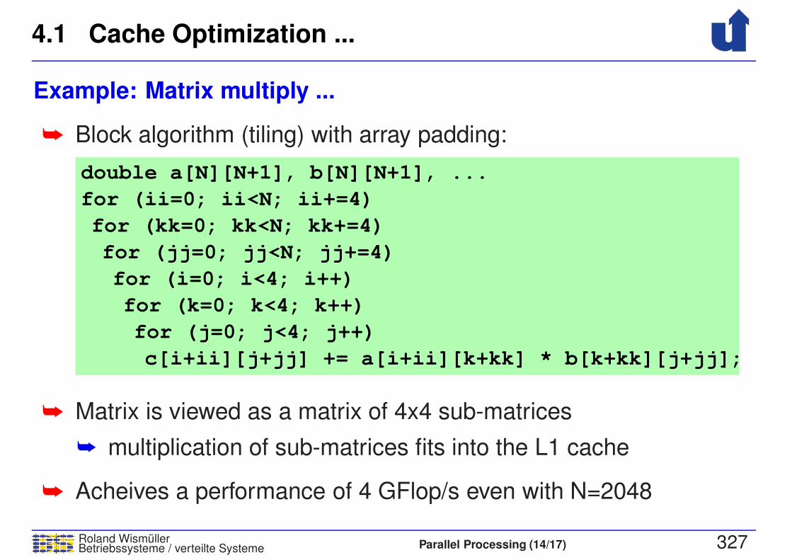
4.1 Cache Optimization ...
Roland WismullerBetriebssysteme / verteilte Systeme Parallel Processing (14/17) 327
Example: Matrix multiply ...
➥ Block algorithm (tiling) with array padding:
double a[N][N+1], b[N][N+1], ...
for (ii=0; ii<N; ii+=4)
for (kk=0; kk<N; kk+=4)
for (jj=0; jj<N; jj+=4)
for (i=0; i<4; i++)
for (k=0; k<4; k++)
for (j=0; j<4; j++)
c[i+ii][j+jj] += a[i+ii][k+kk] * b[k+kk][j+jj];
➥ Matrix is viewed as a matrix of 4x4 sub-matrices
➥ multiplication of sub-matrices fits into the L1 cache
➥ Acheives a performance of 4 GFlop/s even with N=2048
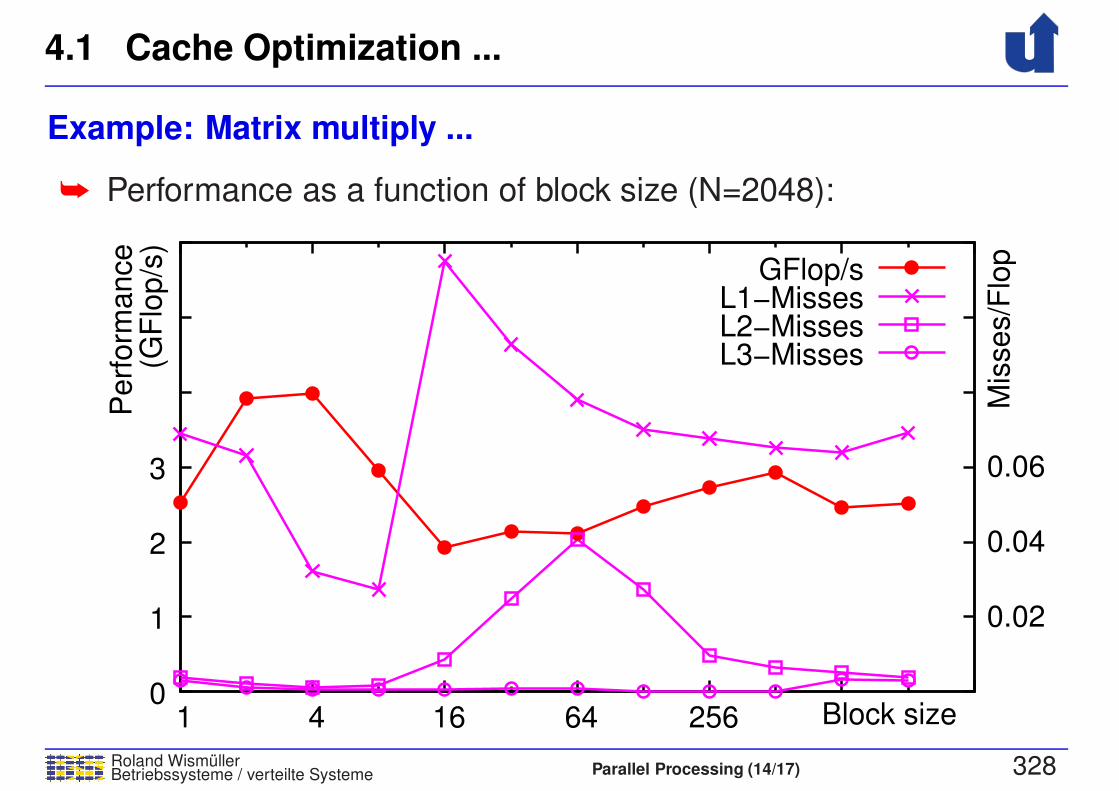
4.1 Cache Optimization ...
Roland WismullerBetriebssysteme / verteilte Systeme Parallel Processing (14/17) 328
Example: Matrix multiply ...
➥ Performance as a function of block size (N=2048):
Mis
ses/F
lop
0.06
0.04
0.02
(GF
lop/s
)P
erf
orm
ance
Block size 0
1
2
3
1 4 16 64 256
GFlop/sL1−MissesL2−MissesL3−Misses

4.1 Cache Optimization ...
Roland WismullerBetriebssysteme / verteilte Systeme Parallel Processing (14/17) 329
Example: Matrix multiply ...
➥ Scalability of performance for different matrix sizes:
Mis
ses/F
lop
0.01
0.02
N
(GF
lop/s
)P
erf
orm
ance
GFlop/sL1−MissesL2−MissesL3−Misses
0
1
2
3
256 512 1024 2048
4.1 Cache Optimization ...
Roland WismullerBetriebssysteme / verteilte Systeme Parallel Processing (14/17) 330
Cache optimization for parallel computers
➥ Cache optimization is especially important for parallel computers
(UMA and NUMA)
➥ larger difference between the access times of cache and main
memory
➥ concurrency conflicts when accessing main memory
➥ Additional problem with parallel computers: false sharing
➥ several variables, which do not have a logical association, can
(by chance) be stored in the same cache line
➥ write accesses to these variables lead to frequent cache
invalidations (due to the cache coherence protocol)
➥ performance degrades drastically
4.1 Cache Optimization ...
Roland WismullerBetriebssysteme / verteilte Systeme Parallel Processing (14/17) 331
Example for false sharing: parallel summation of an array(☞ 04/false.cpp)
➥ Global variable double sum[P] for the partial sums
➥ Version 1: thread i adds to sum[i]
➥ run-time(∗) with 4 threads: 0.4 s, sequentially: 0.24 s !
➥ performance loss due to false sharing: the variables sum[i]
are located in the same cache line
➥ Version 2: thread i first adds to a local variable and stores theresult to sum[i] at the end
➥ run-time(∗) with 4 threads: 0.09 s
➥ Rule: variables that are used by different threads should beseparated in main memory (e.g., use padding)!
(∗) 8000 x 8000 matrix, Intel Xeon 2.66 GHz, without compiler optimization

4.2 Optimization of Communication
Roland WismullerBetriebssysteme / verteilte Systeme Parallel Processing (14/17) 332
Combining messages
➥ The time for sending short messages is dominated by the
(software) latency
➥ i.e., a long message is “cheaper” than several short ones!
➥ Example: PC cluster in the lab H-A 4111 with MPICH2
➥ 32 messages with 32 Byte each need 32 · 145 = 4640µs
➥ one message with 1024 Byte needs only 159µs
➥ Thus: combine the data to be sent into as few messages as
possible
➥ where applicable, this can also be done with communication in
loops (hoisting)

4.2 Optimization of Communication ...
Roland WismullerBetriebssysteme / verteilte Systeme Parallel Processing (14/17) 333
Hoisting of communication calls
for (i=0; i<N; i++) {
}
recv(&b, 1, P1);
a[i] = a[i] + b;
recv(b, N, P1);
for (i=0; i<N; i++) {
a[i] = a[i] + b[i];}
for (i=0; i<N; i++) {
}
b = f(..., i);
send(&b, 1, P2);
for (i=0; i<N; i++) {
b[i] = f(..., i);}
send(b, N, P2);
➥ Send operations are hoisted past the end of the loop,
receive operations are hoisted before the beginning of the loop
➥ Prerequisite: variables are not modified in the loop (sending
process) or not used in the loop (receiving process)
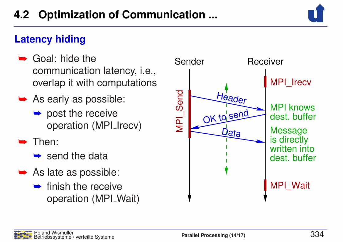
4.2 Optimization of Communication ...
Roland WismullerBetriebssysteme / verteilte Systeme Parallel Processing (14/17) 334
Latency hiding
➥ Goal: hide the
communication latency, i.e.,
overlap it with computations
➥ As early as possible:
➥ post the receive
operation (MPI Irecv)
➥ Then:
➥ send the data
➥ As late as possible:
➥ finish the receive
operation (MPI Wait)
Sender Receiver
MP
I_S
end
MPI_Irecv
MPI_Wait
MPI knowsdest. buffer
Messageis directlywritten intodest. buffer
Header
OK to send
Data

4.3 A Story from Practice
Roland WismullerBetriebssysteme / verteilte Systeme Parallel Processing (14/17) 335
Gauss/Seidel with MPICH (version 1) on Intel Pentium 4
➥ Intended course of execution of the parallel program:
P2
P3
P1
P0
Flow of the communication
i=1: MPI_Irecv()
i=2: MPI_Bsend()
i=n−1: MPI_Wait()of the ’i’−loop
at the beginning
Iteration of’k’−loop
Iteration of’i’−loop
: P0
P1
i=2
i=1 i=n−1
i=n−1i=1
i=2

4.3 A Story from Practice ...
Roland WismullerBetriebssysteme / verteilte Systeme Parallel Processing (14/17) 336
Gauss/Seidel with MPICH (version 1) on Intel Pentium 4 ...
➥ Actual temporal behavior (Jumpshot):
MPI_Bsend
MPI_Wait
➥ Speedup only 2.7 (4 proc., 4000x4000 matrix, run-time: 12.3s)
➥ MPI Bsend (buffered send) blocks! Why?

4.3 A Story from Practice ...
Roland WismullerBetriebssysteme / verteilte Systeme Parallel Processing (14/17) 337
Communication in MPICH-p4
➥ The MPI implementation MPICH-p4 is based on TCP/IP
➥ MPICH-p4 retrieves the messages from the operating system’s
TCP buffer and copies it to the process’s receive buffer
➥ However, the MPI library can do this, only if the process
periodically calls (arbitrary) MPI routines
➥ during the compute phase of Gauss/Seidel this is, however,
not the case
➥ If the TCP buffer is not emptied:
➥ the TCP buffer becomes full
➥ TCP flow control blocks the sender process
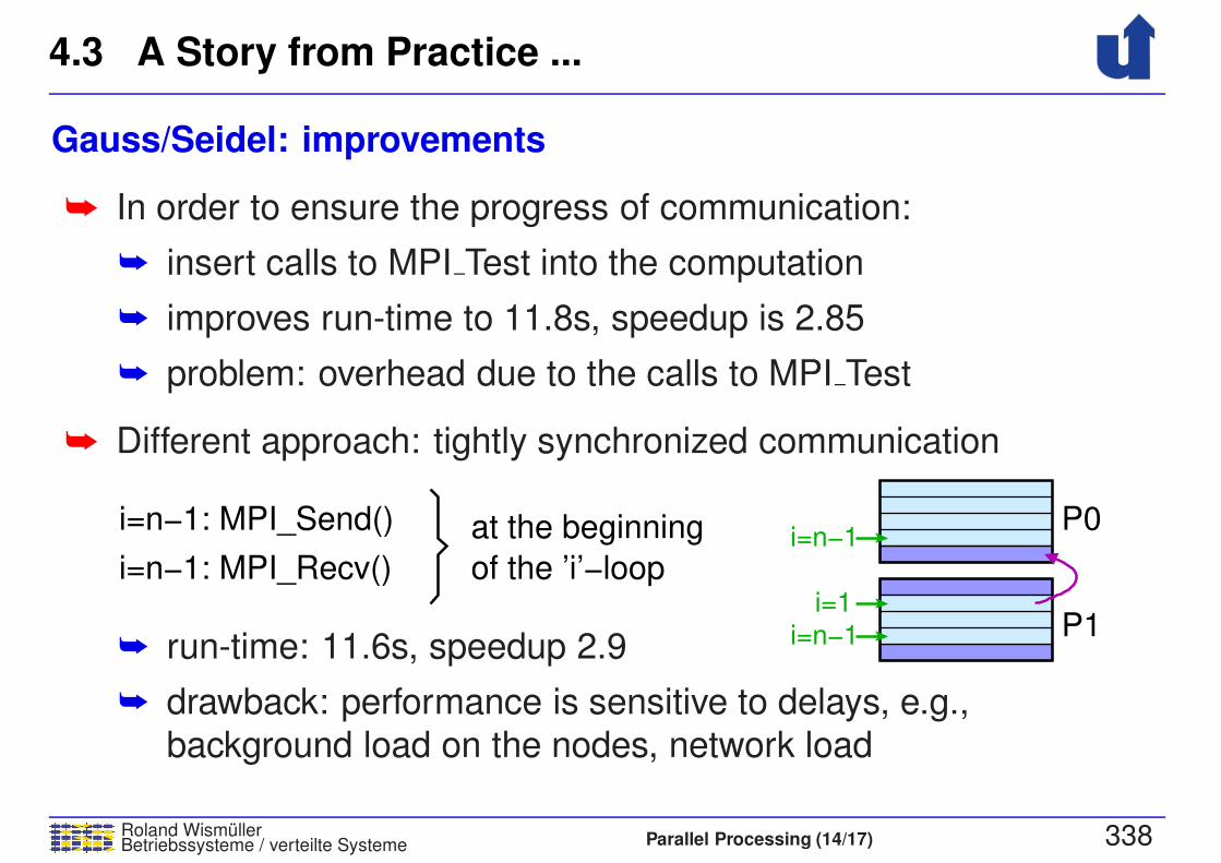
4.3 A Story from Practice ...
Roland WismullerBetriebssysteme / verteilte Systeme Parallel Processing (14/17) 338
Gauss/Seidel: improvements
➥ In order to ensure the progress of communication:
➥ insert calls to MPI Test into the computation
➥ improves run-time to 11.8s, speedup is 2.85
➥ problem: overhead due to the calls to MPI Test
➥ Different approach: tightly synchronized communication
of the ’i’−loop
at the beginningi=n−1: MPI_Send()
i=n−1: MPI_Recv()
P0
P1i=1
i=n−1
i=n−1
➥ run-time: 11.6s, speedup 2.9
➥ drawback: performance is sensitive to delays, e.g.,
background load on the nodes, network load
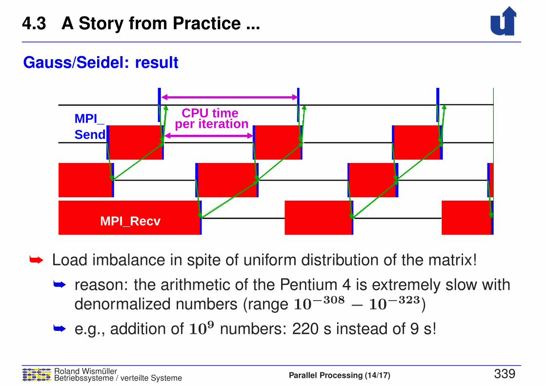
4.3 A Story from Practice ...
Roland WismullerBetriebssysteme / verteilte Systeme Parallel Processing (14/17) 339
Gauss/Seidel: result
MPI_Recv
MPI_Send
CPU timeper iteration
➥ Load imbalance in spite of uniform distribution of the matrix!
➥ reason: the arithmetic of the Pentium 4 is extremely slow with
denormalized numbers (range 10−308 − 10−323)
➥ e.g., addition of 109 numbers: 220 s instead of 9 s!

4.3 A Story from Practice ...
Roland WismullerBetriebssysteme / verteilte Systeme Parallel Processing (14/17) 340
Gauss-Seidel: success!
MPI_Recv
MPI_Send
➥ When initializing the matrix with 10−300 instead of 0, the problem
disappears
➥ Run-time: 7.0 s, speedup: 3.4
➥ Sequential run-time now only 23.8 s instead of 33.6 s
4.3 A Story from Practice ...
Roland WismullerBetriebssysteme / verteilte Systeme Parallel Processing (14/17) 341
Lessons learned:
➥ Latency hiding only works reasonably, when the progress of the
communication is ensured
➥ e.g., with MPI over Myrinet: the network interface card writes
the arriving data directly into the process’s receive buffer
➥ or with MPICH2 (separate thread)
➥ Tightly synchronized communication can be better, but is
susceptible to delays
➥ Load imbalance can also occur when you don’t expect it
➥ the execution times of modern processors are unpredictable

4.4 Summary
Roland WismullerBetriebssysteme / verteilte Systeme Parallel Processing (14/17) 342
➥ Take care of good locality (caches)!
➥ traverse matrices in the oder in which they are stored
➥ avoid powers of two as address increment when sweeping
through memory
➥ use block algorithms
➥ Avoid false sharing!
➥ Combine messages, if possible!
➥ Use latency hiding when the communication library can execute
the receipt of a message “in background”
➥ If send operations are blocking: execute send and receive
operations as synchronously as possible

Roland WismullerBetriebssysteme / verteilte Systeme Parallel Processing (14/17) 343
Parallel ProcessingWS 2017/18
5 Appendix

Roland WismullerBetriebssysteme / verteilte Systeme Parallel Processing (15/17) xvi
Roland Wismuller
Universitat Siegen
Tel.: 0271/740-4050, Buro: H-B 8404
Stand: January 23, 2018
Parallel Processing
WS 2017/18
26.10.2017

5.1 Tutorial: C/C++ for Java Programmers
Roland WismullerBetriebssysteme / verteilte Systeme Parallel Processing (15/17) 344
5.1.1 Fundamentals of C++
➥ Commonalities between C++ and Java:
➥ imperative programming language
➥ syntax is mostly identical
➥ Differences between C++ and Java:
➥ C++ is not purely object oriented
➥ C++ programs are translated directly to machine code (novirtual machine)
➥ Usual file structure of C++ programs:
➥ header files (*.h) contain declarations
➥ types, classes, constants, ...
➥ source files (*.cpp) contain implementations
➥ methods, functions, global variables

5.1.1 Fundamentals of C++ ...
Roland WismullerBetriebssysteme / verteilte Systeme Parallel Processing (15/17) 345
Compilation of C++ programs
init memory
call main()
return result
x.o
Header files(Include files)
Source file(s)
Pre−
processor
Compiler Linker
Initialisation code
hello
Source file(s) Object file(s) Executableprogram
x.cpp
x.h
➥ Preprocessor: embedding of files, expansion of macros
➥ Linker: binds together object files and libraries
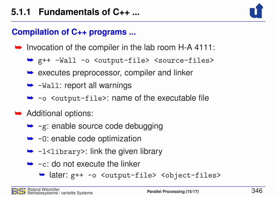
5.1.1 Fundamentals of C++ ...
Roland WismullerBetriebssysteme / verteilte Systeme Parallel Processing (15/17) 346
Compilation of C++ programs ...
➥ Invocation of the compiler in the lab room H-A 4111:
➥ g++ -Wall -o <output-file> <source-files>
➥ executes preprocessor, compiler and linker
➥ -Wall: report all warnings
➥ -o <output-file>: name of the executable file
➥ Additional options:
➥ -g: enable source code debugging
➥ -O: enable code optimization
➥ -l<library>: link the given library
➥ -c: do not execute the linker
➥ later: g++ -o <output-file> <object-files>

5.1.1 Fundamentals of C++ ...
Roland WismullerBetriebssysteme / verteilte Systeme Parallel Processing (15/17) 347
An example: Hello World! (☞ 05/hello.cpp)
Preprocessor directive: insertscontents of file ’iostream’(e.g., declaration of cout)
Return from main program:
Main program
Output of a text
0 = OK, 1,2,...,255: error
Function definition
Use the namespace ’std’
#include <iostream>
return 0;}
sayHello();{
void sayHello(){
using namespace std;
cout << "Hello World\n";}
int main()
➥ Compilation: g++ -Wall -o hello hello.cpp
➥ Start: ./hello

5.1.1 Fundamentals of C++ ...
Roland WismullerBetriebssysteme / verteilte Systeme Parallel Processing (15/17) 348
Syntax
➥ Identical to Java are among others:
➥ declaration of variables and parameters
➥ method calls
➥ control statements (if, while, for, case, return, ...)
➥ simple data types (short, int, double, char, void, ...)
➥ deviations: bool instead of boolean; char has a size of
1 Byte
➥ virtually all operators (+, *, %, <<, ==, ?:, ...)
➥ Very similar to Java are:
➥ arrays
➥ class declarations
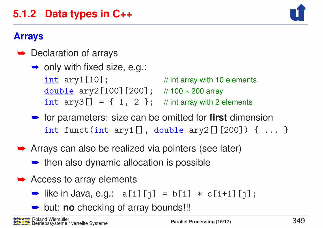
5.1.2 Data types in C++
Roland WismullerBetriebssysteme / verteilte Systeme Parallel Processing (15/17) 349
Arrays
➥ Declaration of arrays
➥ only with fixed size, e.g.:
int ary1[10]; // int array with 10 elements
double ary2[100][200]; // 100 ∗ 200 array
int ary3[] = { 1, 2 }; // int array with 2 elements
➥ for parameters: size can be omitted for first dimension
int funct(int ary1[], double ary2[][200]) { ... }
➥ Arrays can also be realized via pointers (see later)
➥ then also dynamic allocation is possible
➥ Access to array elements
➥ like in Java, e.g.: a[i][j] = b[i] * c[i+1][j];
➥ but: no checking of array bounds!!!

5.1.2 Data types in C++ ...
Roland WismullerBetriebssysteme / verteilte Systeme Parallel Processing (15/17) 350
Classes and objects
➥ Declaration of classes (typically in .h file):
class Example {
private: // private attributes/methods
int attr1; // attribute
void pmeth(double d); // method
public: // public attributes/methods
Example(); // default constructor
Example(int i); // constructor
Example(Example &from); // copy constructor
~Example(); // destructor
int meth(); // method
int attr2; // attribute
static int sattr; // class attribute
};
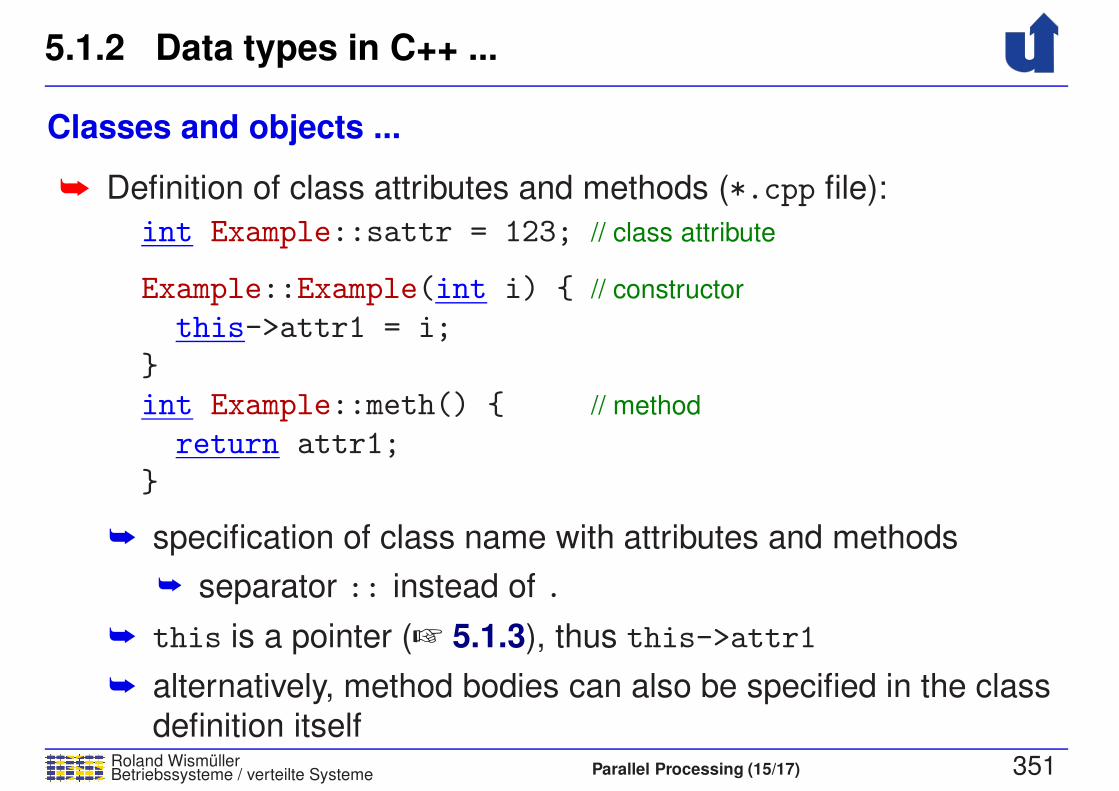
5.1.2 Data types in C++ ...
Roland WismullerBetriebssysteme / verteilte Systeme Parallel Processing (15/17) 351
Classes and objects ...
➥ Definition of class attributes and methods (*.cpp file):
int Example::sattr = 123; // class attribute
Example::Example(int i) { // constructor
this->attr1 = i;
}
int Example::meth() { // method
return attr1;
}
➥ specification of class name with attributes and methods
➥ separator :: instead of .
➥ this is a pointer (☞ 5.1.3), thus this->attr1
➥ alternatively, method bodies can also be specified in the class
definition itself
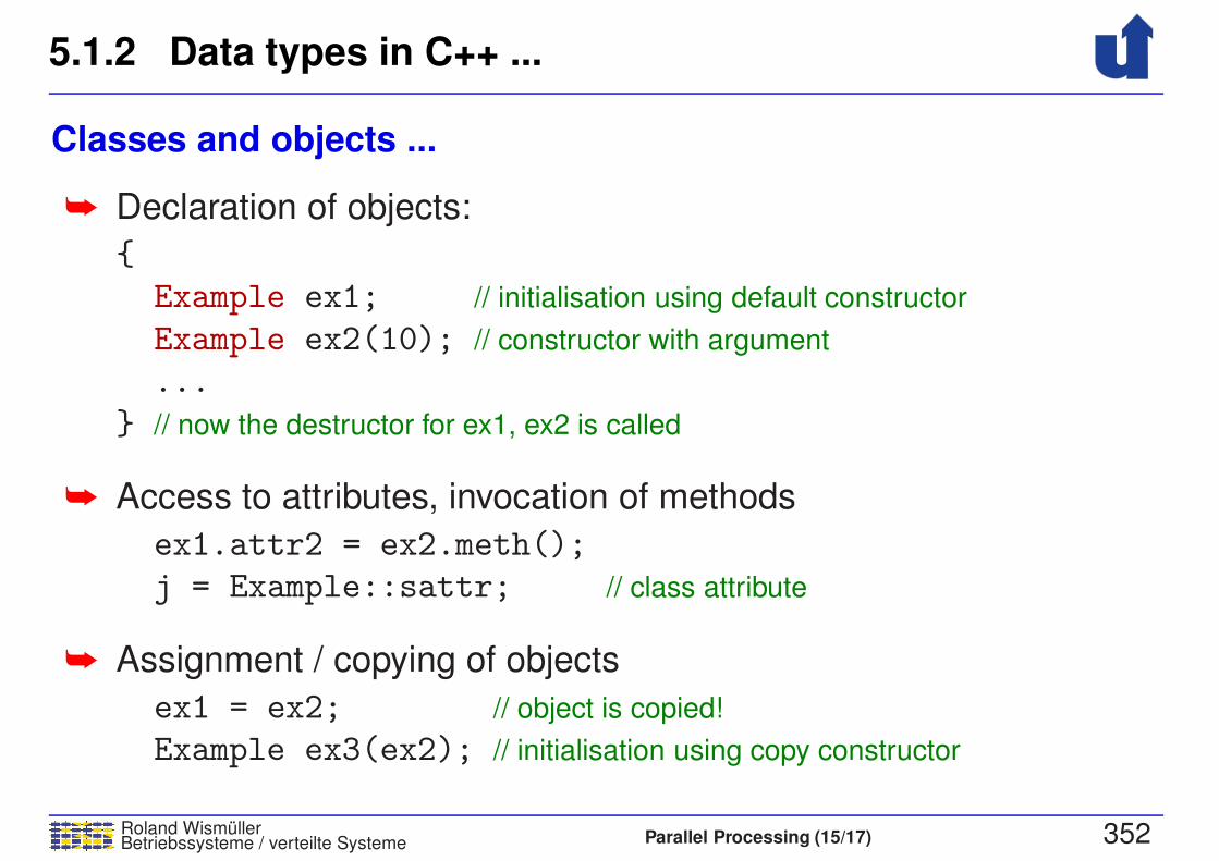
5.1.2 Data types in C++ ...
Roland WismullerBetriebssysteme / verteilte Systeme Parallel Processing (15/17) 352
Classes and objects ...
➥ Declaration of objects:
{
Example ex1; // initialisation using default constructor
Example ex2(10); // constructor with argument
...
} // now the destructor for ex1, ex2 is called
➥ Access to attributes, invocation of methods
ex1.attr2 = ex2.meth();
j = Example::sattr; // class attribute
➥ Assignment / copying of objects
ex1 = ex2; // object is copied!
Example ex3(ex2); // initialisation using copy constructor
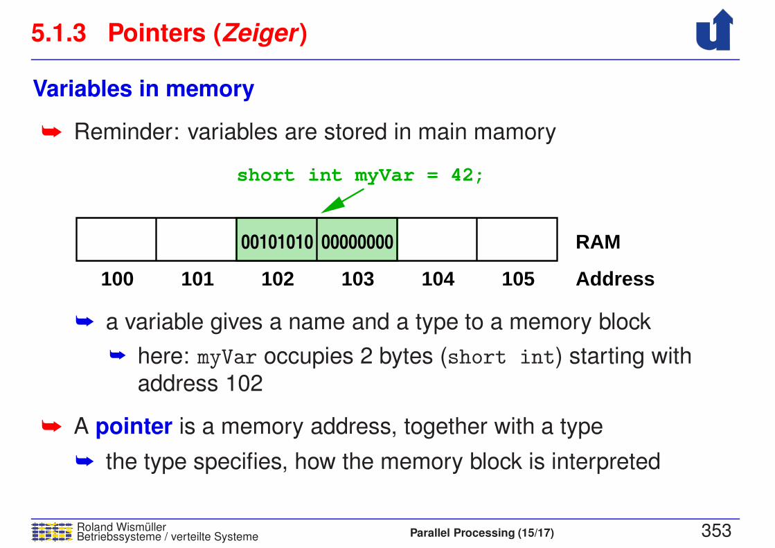
5.1.3 Pointers (Zeiger)
Roland WismullerBetriebssysteme / verteilte Systeme Parallel Processing (15/17) 353
Variables in memory
➥ Reminder: variables are stored in main mamory
RAM00000000
100 105104103102101
00101010
short int myVar = 42;
Address
➥ a variable gives a name and a type to a memory block
➥ here: myVar occupies 2 bytes (short int) starting with
address 102
➥ A pointer is a memory address, together with a type
➥ the type specifies, how the memory block is interpreted
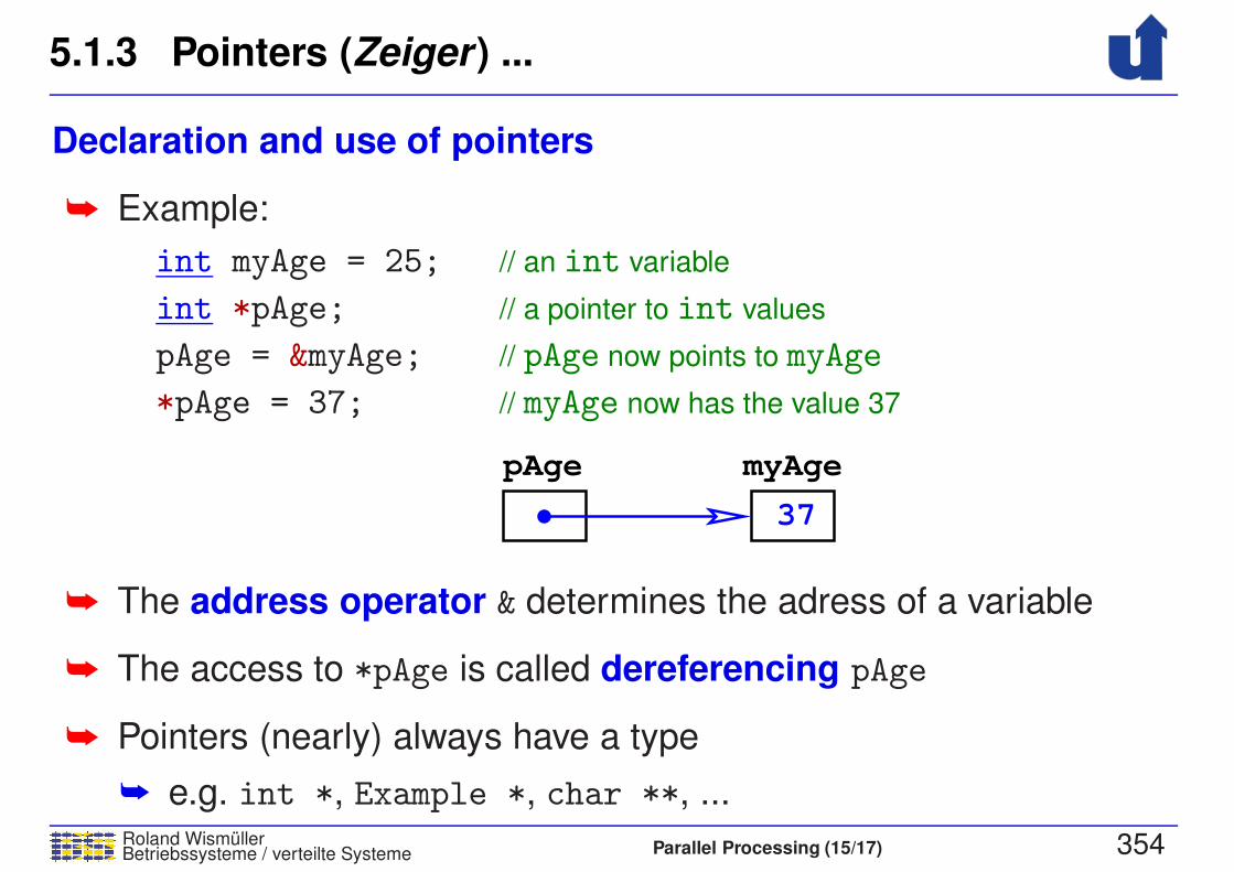
5.1.3 Pointers (Zeiger) ...
Roland WismullerBetriebssysteme / verteilte Systeme Parallel Processing (15/17) 354
Declaration and use of pointers
➥ Example:
int myAge = 25; // an int variable
int *pAge; // a pointer to int values
pAge = &myAge; // pAge now points to myAge
*pAge = 37; // myAge now has the value 37
pAge myAge
37
➥ The address operator & determines the adress of a variable
➥ The access to *pAge is called dereferencing pAge
➥ Pointers (nearly) always have a type
➥ e.g. int *, Example *, char **, ...
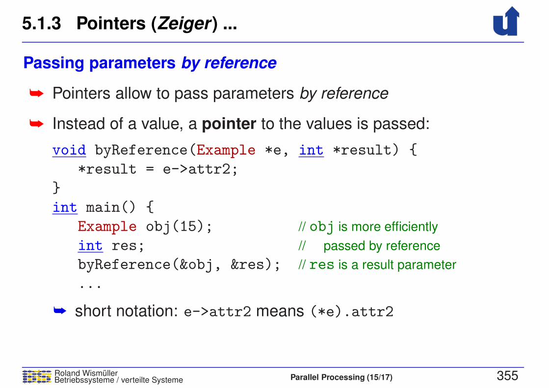
5.1.3 Pointers (Zeiger) ...
Roland WismullerBetriebssysteme / verteilte Systeme Parallel Processing (15/17) 355
Passing parameters by reference
➥ Pointers allow to pass parameters by reference
➥ Instead of a value, a pointer to the values is passed:
void byReference(Example *e, int *result) {
*result = e->attr2;
}
int main() {
Example obj(15); // obj is more efficiently
int res; // passed by reference
byReference(&obj, &res); // res is a result parameter
...
➥ short notation: e->attr2 means (*e).attr2

5.1.3 Pointers (Zeiger) ...
Roland WismullerBetriebssysteme / verteilte Systeme Parallel Processing (15/17) 356
void pointers and type conversion
➥ C++ also allows the use of generic pointers
➥ just a memory addess without type information
➥ declared type is void * (pointer to void)
➥ Dereferencing only possible after a type conversion
➥ caution: no type safety / type check!
➥ Often used for generic parameters of functions:
void bsp(int type, void *arg) {
if (type == 1) {
double d = *(double *)arg; // arg must first be converted
// to double *
} else {
int i = *(int *)arg; // int argument

5.1.3 Pointers (Zeiger) ...
Roland WismullerBetriebssysteme / verteilte Systeme Parallel Processing (15/17) 357
Arrays and pointers
➥ C++ does not distinguish between one-dimensional arrays and
pointers (with the exception of the declaration)
➥ Consequences:
➥ array variables can be used like (constant) pointers
➥ pointer variables can be indexed
int a[3] = { 1, 2, 3 };
int b = *a; // equivalent to: b = a[0]
int c = *(a+1); // equivalent to: c = a[1]
int *p = a; // equivalent to: int *p = &a[0]
int d = p[2]; // d = a[2]
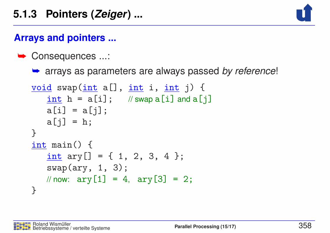
5.1.3 Pointers (Zeiger) ...
Roland WismullerBetriebssysteme / verteilte Systeme Parallel Processing (15/17) 358
Arrays and pointers ...
➥ Consequences ...:
➥ arrays as parameters are always passed by reference!
void swap(int a[], int i, int j) {
int h = a[i]; // swap a[i] and a[j]
a[i] = a[j];
a[j] = h;
}
int main() {
int ary[] = { 1, 2, 3, 4 };
swap(ary, 1, 3);
// now: ary[1] = 4, ary[3] = 2;
}
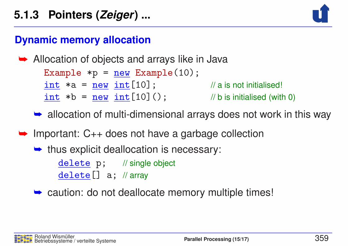
5.1.3 Pointers (Zeiger) ...
Roland WismullerBetriebssysteme / verteilte Systeme Parallel Processing (15/17) 359
Dynamic memory allocation
➥ Allocation of objects and arrays like in Java
Example *p = new Example(10);
int *a = new int[10]; // a is not initialised!
int *b = new int[10](); // b is initialised (with 0)
➥ allocation of multi-dimensional arrays does not work in this way
➥ Important: C++ does not have a garbage collection
➥ thus explicit deallocation is necessary:
delete p; // single object
delete[] a; // array
➥ caution: do not deallocate memory multiple times!
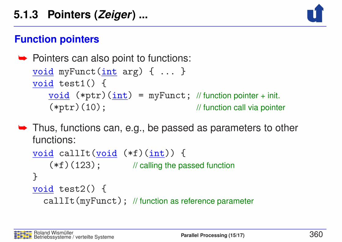
5.1.3 Pointers (Zeiger) ...
Roland WismullerBetriebssysteme / verteilte Systeme Parallel Processing (15/17) 360
Function pointers
➥ Pointers can also point to functions:
void myFunct(int arg) { ... }
void test1() {
void (*ptr)(int) = myFunct; // function pointer + init.
(*ptr)(10); // function call via pointer
➥ Thus, functions can, e.g., be passed as parameters to otherfunctions:
void callIt(void (*f)(int)) {
(*f)(123); // calling the passed function
}
void test2() {
callIt(myFunct); // function as reference parameter
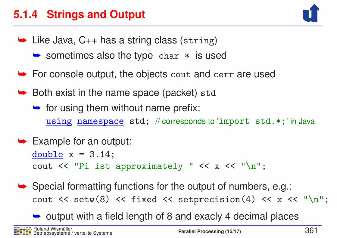
5.1.4 Strings and Output
Roland WismullerBetriebssysteme / verteilte Systeme Parallel Processing (15/17) 361
➥ Like Java, C++ has a string class (string)
➥ sometimes also the type char * is used
➥ For console output, the objects cout and cerr are used
➥ Both exist in the name space (packet) std
➥ for using them without name prefix:
using namespace std; // corresponds to ’import std.*;’ in Java
➥ Example for an output:
double x = 3.14;
cout << "Pi ist approximately " << x << "\n";
➥ Special formatting functions for the output of numbers, e.g.:
cout << setw(8) << fixed << setprecision(4) << x << "\n";
➥ output with a field length of 8 and exacly 4 decimal places

5.1.5 Further specifics of C++
Roland WismullerBetriebssysteme / verteilte Systeme Parallel Processing (15/17) 362
➥ Global variables
➥ are declared outside any function or method
➥ live during the complete program execution
➥ are accessible by all functions
➥ Global variables and functions can be used only after thedeclaration
➥ thus, for functions we have function prototypes
int funcB(int n); // function prototype
int funcA() { // function definition
return funcB(10);
}
int funcB(int n) { // function definition
return n * n;
}
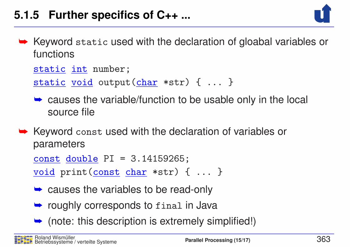
5.1.5 Further specifics of C++ ...
Roland WismullerBetriebssysteme / verteilte Systeme Parallel Processing (15/17) 363
➥ Keyword static used with the declaration of gloabal variables or
functions
static int number;
static void output(char *str) { ... }
➥ causes the variable/function to be usable only in the local
source file
➥ Keyword const used with the declaration of variables or
parameters
const double PI = 3.14159265;
void print(const char *str) { ... }
➥ causes the variables to be read-only
➥ roughly corresponds to final in Java
➥ (note: this description is extremely simplified!)
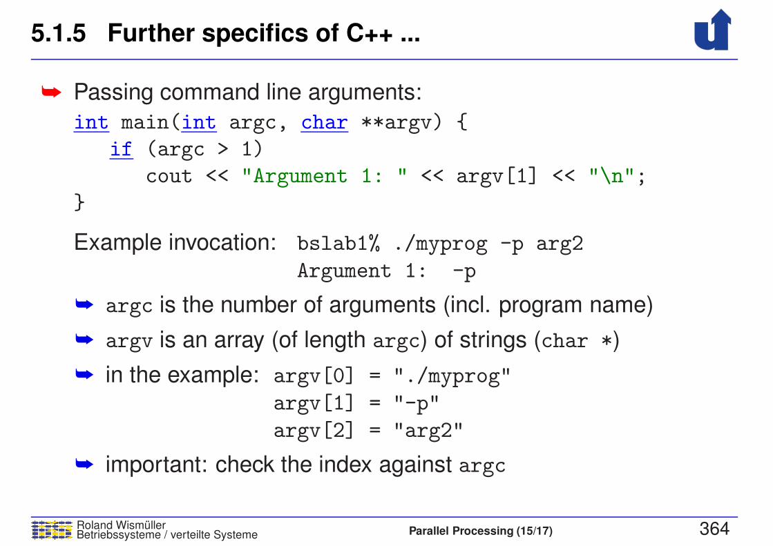
5.1.5 Further specifics of C++ ...
Roland WismullerBetriebssysteme / verteilte Systeme Parallel Processing (15/17) 364
➥ Passing command line arguments:
int main(int argc, char **argv) {
if (argc > 1)
cout << "Argument 1: " << argv[1] << "\n";
}
Example invocation: bslab1% ./myprog -p arg2
Argument 1: -p
➥ argc is the number of arguments (incl. program name)
➥ argv is an array (of length argc) of strings (char *)
➥ in the example: argv[0] = "./myprog"
argv[1] = "-p"
argv[2] = "arg2"
➥ important: check the index against argc
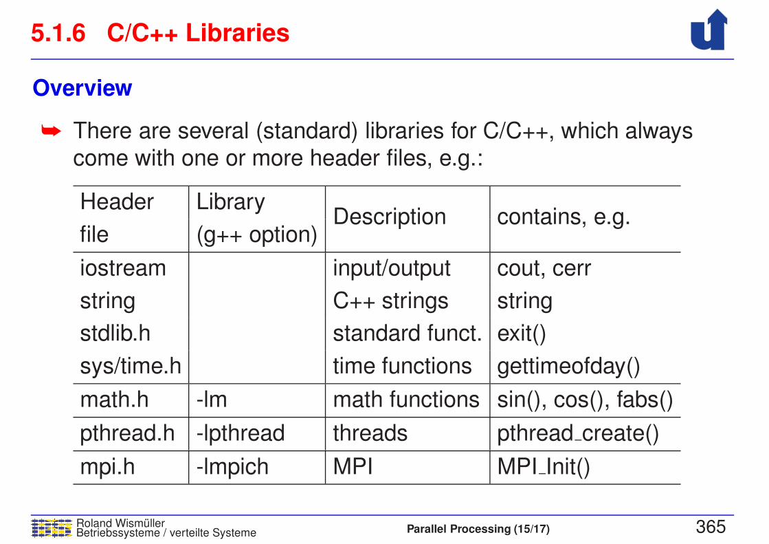
5.1.6 C/C++ Libraries
Roland WismullerBetriebssysteme / verteilte Systeme Parallel Processing (15/17) 365
Overview
➥ There are several (standard) libraries for C/C++, which always
come with one or more header files, e.g.:
Header Library
file (g++ option)Description contains, e.g.
iostream input/output cout, cerr
string C++ strings string
stdlib.h standard funct. exit()
sys/time.h time functions gettimeofday()
math.h -lm math functions sin(), cos(), fabs()
pthread.h -lpthread threads pthread create()
mpi.h -lmpich MPI MPI Init()
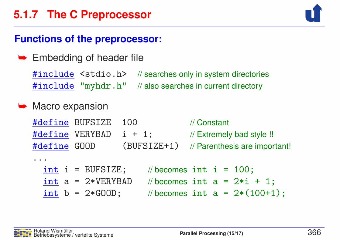
5.1.7 The C Preprocessor
Roland WismullerBetriebssysteme / verteilte Systeme Parallel Processing (15/17) 366
Functions of the preprocessor:
➥ Embedding of header file
#include <stdio.h> // searches only in system directories
#include "myhdr.h" // also searches in current directory
➥ Macro expansion
#define BUFSIZE 100 // Constant
#define VERYBAD i + 1; // Extremely bad style !!
#define GOOD (BUFSIZE+1) // Parenthesis are important!
...
int i = BUFSIZE; // becomes int i = 100;
int a = 2*VERYBAD // becomes int a = 2*i + 1;
int b = 2*GOOD; // becomes int a = 2*(100+1);
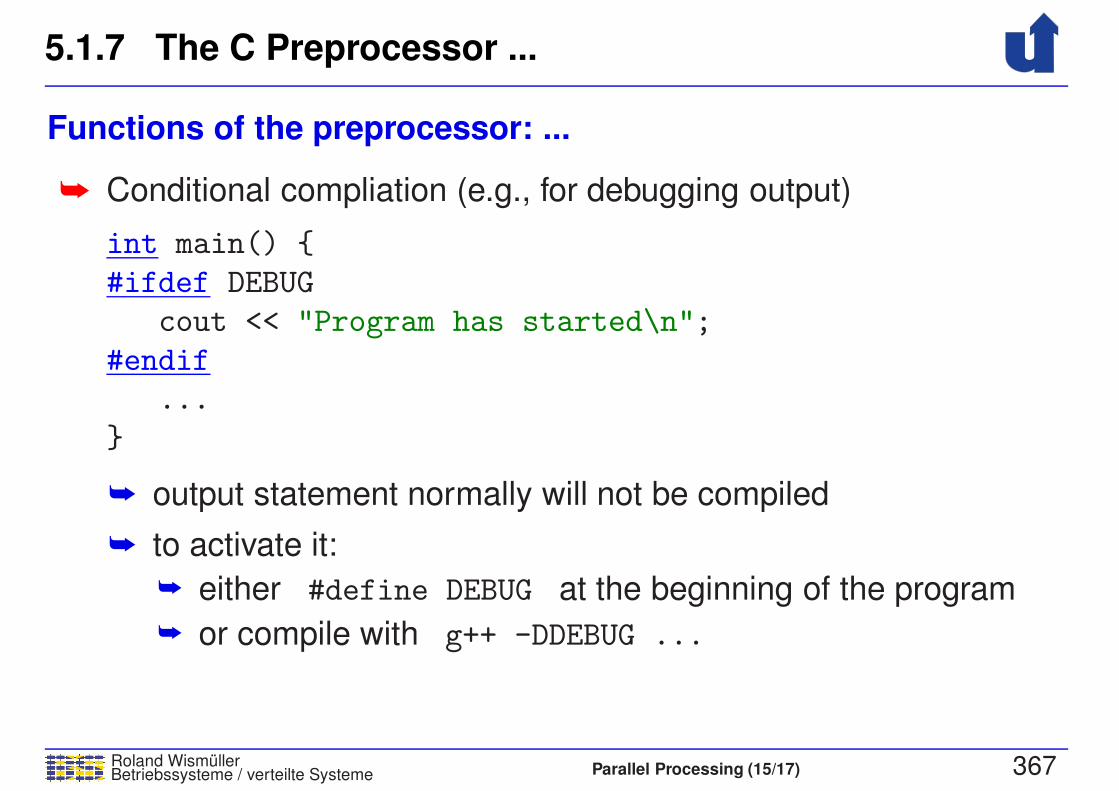
5.1.7 The C Preprocessor ...
Roland WismullerBetriebssysteme / verteilte Systeme Parallel Processing (15/17) 367
Functions of the preprocessor: ...
➥ Conditional compliation (e.g., for debugging output)
int main() {
#ifdef DEBUG
cout << "Program has started\n";
#endif
...
}
➥ output statement normally will not be compiled
➥ to activate it:
➥ either #define DEBUG at the beginning of the program
➥ or compile with g++ -DDEBUG ...

Roland WismullerBetriebssysteme / verteilte Systeme Parallel Processing (16/17) xvii
Roland Wismuller
Universitat Siegen
Tel.: 0271/740-4050, Buro: H-B 8404
Stand: January 23, 2018
Parallel Processing
WS 2017/18
20.11.2017
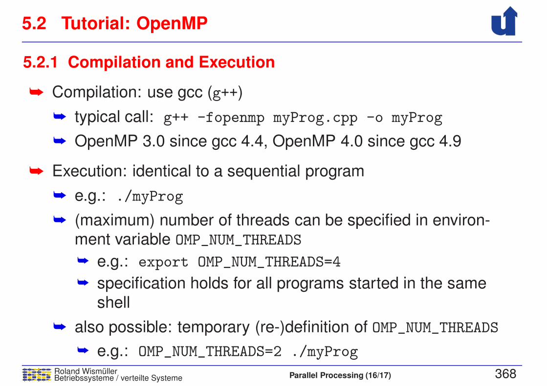
5.2 Tutorial: OpenMP
Roland WismullerBetriebssysteme / verteilte Systeme Parallel Processing (16/17) 368
5.2.1 Compilation and Execution
➥ Compilation: use gcc (g++)
➥ typical call: g++ -fopenmp myProg.cpp -o myProg
➥ OpenMP 3.0 since gcc 4.4, OpenMP 4.0 since gcc 4.9
➥ Execution: identical to a sequential program
➥ e.g.: ./myProg
➥ (maximum) number of threads can be specified in environ-ment variable OMP_NUM_THREADS
➥ e.g.: export OMP_NUM_THREADS=4
➥ specification holds for all programs started in the same
shell
➥ also possible: temporary (re-)definition of OMP_NUM_THREADS
➥ e.g.: OMP_NUM_THREADS=2 ./myProg
5.2.2 Debugging
Roland WismullerBetriebssysteme / verteilte Systeme Parallel Processing (16/17) 369
➥ There are only few debuggers that fully support OpenMP
➥ e.g., Totalview
➥ requires tight cooperation between compiler and debugger
➥ On the PCs in the lab room H-A 4111:
➥ gdb and ddd allow halfway reasonable debugging
➥ they support multiple threads
➥ gdb: textual debugger (standard LINUX debugger)
➥ ddd: graphical front end for gdb
➥ more comfortable, but more “heavy-weight”
➥ On the HorUS cluster: totalview
➥ graphical debugger
➥ supports both OpenMP and MPI
5.2.2 Debugging ...
Roland WismullerBetriebssysteme / verteilte Systeme Parallel Processing (16/17) 370
➥ Prerequisite: compilation with debugging information
➥ sequential: g++ -g -o myProg myProg.cpp
➥ with OpenMP: g++ -g -fopenmp ...
➥ Limited(!) debugging is also possible in combination with
optimization
➥ however, the debugger may show unexpected behavior
➥ if possible: switch off the optimization
➥ g++ -g -O0 ...
5.2.2 Debugging ...
Roland WismullerBetriebssysteme / verteilte Systeme Parallel Processing (16/17) 371
Important functions of a debugger (Examples for gdb):
➥ Start the programm: run arg1 arg2
➥ Set breakpoints on code lines: break file.cpp:35
➥ Set breakpoints on functions: break myFunc
➥ Show the procedure call stack: where
➥ Navigate in the procedure call stack: up bzw. down
➥ Show the contents of variables: print i
➥ Change the contents of variables: set variable i=i*15
➥ Continue the program (after a breakpoint): continue
➥ Single-step execution: step bzw. next
5.2.2 Debugging ...
Roland WismullerBetriebssysteme / verteilte Systeme Parallel Processing (16/17) 372
Important functions of a debugger (Examples for gdb): ...
➥ Show all threads: info threads
➥ Select a thread: thread 2
➥ subsequent commands typically only affect the selected thread
➥ Source code listing: list
➥ Help: help
➥ Exit the debugger: quit
➥ All commands can also be abbreviated in gdb
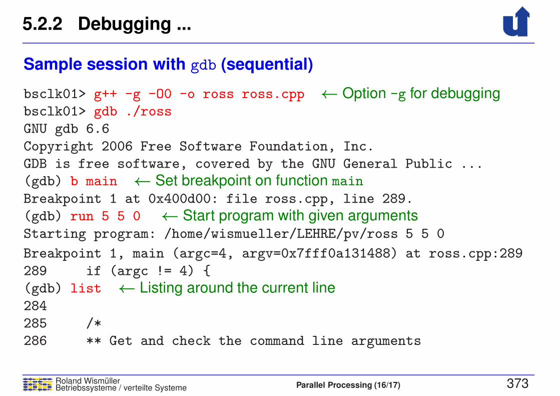
5.2.2 Debugging ...
Roland WismullerBetriebssysteme / verteilte Systeme Parallel Processing (16/17) 373
Sample session with gdb (sequential)
bsclk01> g++ -g -O0 -o ross ross.cpp ← Option -g for debuggingbsclk01> gdb ./ross
GNU gdb 6.6
Copyright 2006 Free Software Foundation, Inc.
GDB is free software, covered by the GNU General Public ...
(gdb) b main ← Set breakpoint on function main
Breakpoint 1 at 0x400d00: file ross.cpp, line 289.
(gdb) run 5 5 0 ← Start program with given argumentsStarting program: /home/wismueller/LEHRE/pv/ross 5 5 0
Breakpoint 1, main (argc=4, argv=0x7fff0a131488) at ross.cpp:289
289 if (argc != 4) {
(gdb) list ← Listing around the current line284
285 /*
286 ** Get and check the command line arguments

5.2.2 Debugging ...
Roland WismullerBetriebssysteme / verteilte Systeme Parallel Processing (16/17) 374
287 */
288
289 if (argc != 4) {
290 cerr << "Usage: ross <size_x> <size_y> ...
291 cerr << " <size_x> <size_y>: size...
292 cerr << " <all>: 0 = compute one ...
293 cerr << " 1 = compute all ...
(gdb) b 315 ← Set breakpoint on line 315Breakpoint 2 at 0x400e59: file ross.cpp, line 315.
(gdb) c ← Continue the programContinuing.
Breakpoint 2, main (argc=4, argv=0x7fff0a131488) at ross.cpp:315
315 num_moves = Find_Route(size_x, size_y, moves);
(gdb) n ← Execute next source line (here: 315)320 if (num_moves >= 0) {
(gdb) p num moves ← Print contents of num moves
$1 = 24
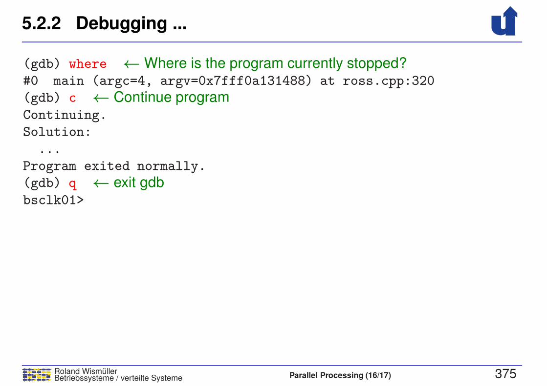
5.2.2 Debugging ...
Roland WismullerBetriebssysteme / verteilte Systeme Parallel Processing (16/17) 375
(gdb) where ←Where is the program currently stopped?#0 main (argc=4, argv=0x7fff0a131488) at ross.cpp:320
(gdb) c ← Continue programContinuing.
Solution:
...
Program exited normally.
(gdb) q ← exit gdbbsclk01>
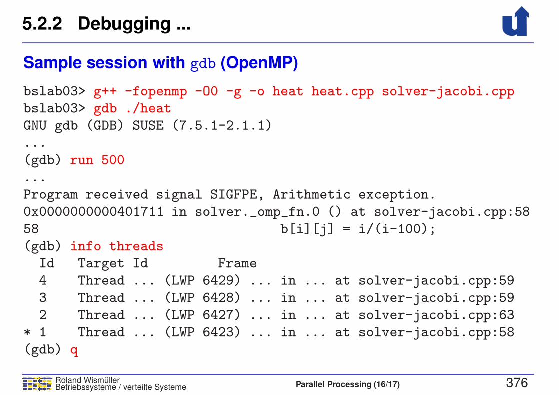
5.2.2 Debugging ...
Roland WismullerBetriebssysteme / verteilte Systeme Parallel Processing (16/17) 376
Sample session with gdb (OpenMP)
bslab03> g++ -fopenmp -O0 -g -o heat heat.cpp solver-jacobi.cppbslab03> gdb ./heat
GNU gdb (GDB) SUSE (7.5.1-2.1.1)
...
(gdb) run 500
...
Program received signal SIGFPE, Arithmetic exception.
0x0000000000401711 in solver._omp_fn.0 () at solver-jacobi.cpp:58
58 b[i][j] = i/(i-100);
(gdb) info threadsId Target Id Frame
4 Thread ... (LWP 6429) ... in ... at solver-jacobi.cpp:59
3 Thread ... (LWP 6428) ... in ... at solver-jacobi.cpp:59
2 Thread ... (LWP 6427) ... in ... at solver-jacobi.cpp:63
* 1 Thread ... (LWP 6423) ... in ... at solver-jacobi.cpp:58
(gdb) q
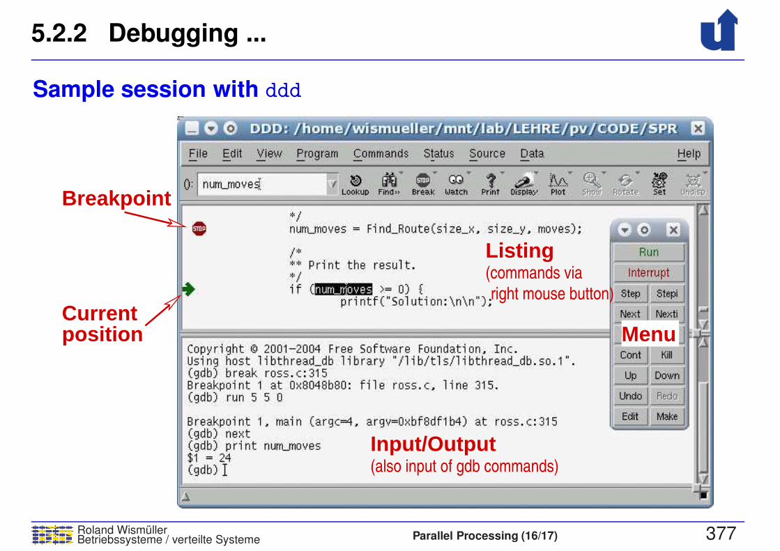
5.2.2 Debugging ...
Roland WismullerBetriebssysteme / verteilte Systeme Parallel Processing (16/17) 377
Sample session with ddd
MenuCurrentposition
Breakpoint
Listing(commands via
right mouse button)
Input/Output(also input of gdb commands)
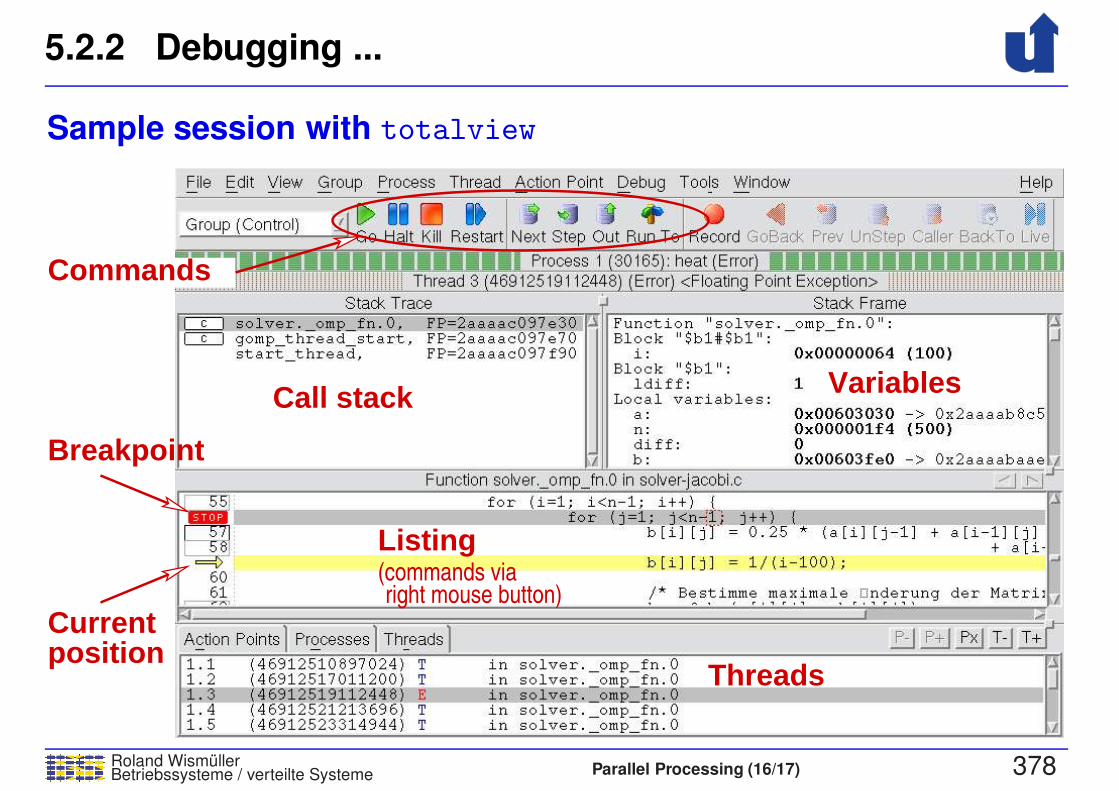
5.2.2 Debugging ...
Roland WismullerBetriebssysteme / verteilte Systeme Parallel Processing (16/17) 378
Sample session with totalview
Breakpoint
Currentposition
Listing
right mouse button)(commands via
Threads
Call stack Variables
Commands
5.2 Tutorial: OpenMP ...
Roland WismullerBetriebssysteme / verteilte Systeme Parallel Processing (16/17) 379
5.2.3 Performance Analysis
➥ Typically: instrumentation of the generated executable code
during/after the compilation
➥ insertion of code at important places in the program
➥ in order monitor relevant events
➥ e.g., at the beginning/end of parallel regions, barriers, ...
➥ during the execution, the events will be
➥ individually logged in a trace file (Spurdatei)
➥ or already summarized into a profile
➥ Evaluation is done after the program terminates
➥ c.f. Section 1.9.6
➥ In the H-A 4111: Scalasca
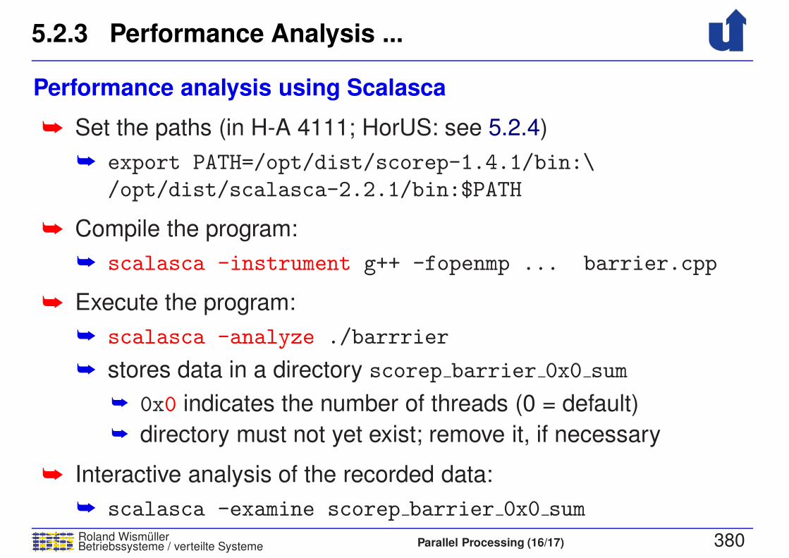
5.2.3 Performance Analysis ...
Roland WismullerBetriebssysteme / verteilte Systeme Parallel Processing (16/17) 380
Performance analysis using Scalasca
➥ Set the paths (in H-A 4111; HorUS: see 5.2.4)
➥ export PATH=/opt/dist/scorep-1.4.1/bin:\
/opt/dist/scalasca-2.2.1/bin:$PATH
➥ Compile the program:
➥ scalasca -instrument g++ -fopenmp ... barrier.cpp
➥ Execute the program:
➥ scalasca -analyze ./barrrier
➥ stores data in a directory scorep barrier 0x0 sum
➥ 0x0 indicates the number of threads (0 = default)
➥ directory must not yet exist; remove it, if necessary
➥ Interactive analysis of the recorded data:
➥ scalasca -examine scorep barrier 0x0 sum

5.2.3 Performance Analysis ...
Roland WismullerBetriebssysteme / verteilte Systeme Parallel Processing (16/17) 381
Performance analysis using Scalasca: Example from slide 217
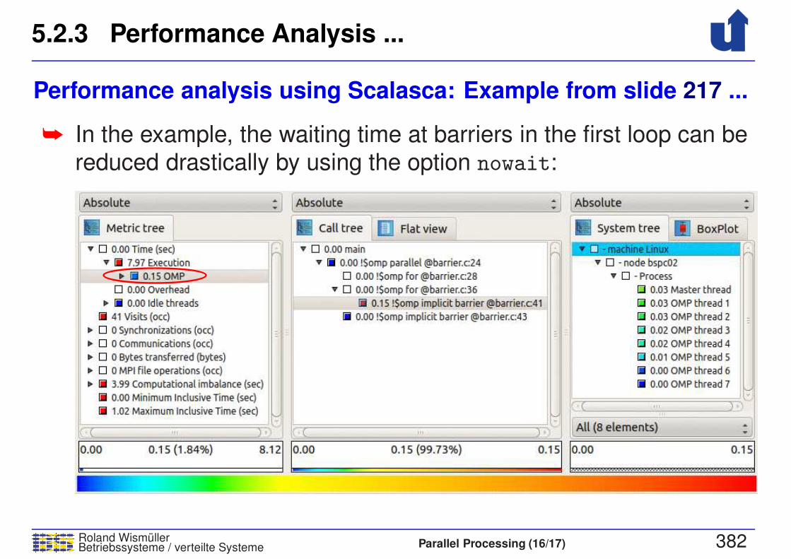
5.2.3 Performance Analysis ...
Roland WismullerBetriebssysteme / verteilte Systeme Parallel Processing (16/17) 382
Performance analysis using Scalasca: Example from slide 217 ...
➥ In the example, the waiting time at barriers in the first loop can be
reduced drastically by using the option nowait:
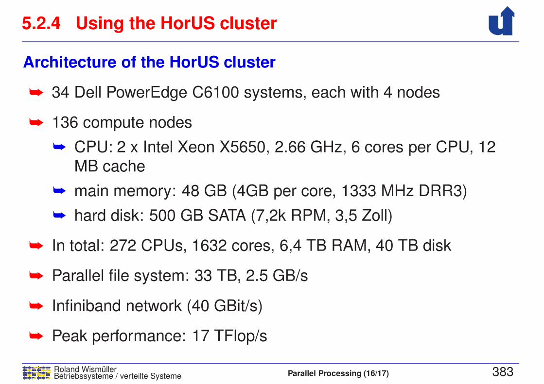
5.2.4 Using the HorUS cluster
Roland WismullerBetriebssysteme / verteilte Systeme Parallel Processing (16/17) 383
Architecture of the HorUS cluster
➥ 34 Dell PowerEdge C6100 systems, each with 4 nodes
➥ 136 compute nodes
➥ CPU: 2 x Intel Xeon X5650, 2.66 GHz, 6 cores per CPU, 12
MB cache
➥ main memory: 48 GB (4GB per core, 1333 MHz DRR3)
➥ hard disk: 500 GB SATA (7,2k RPM, 3,5 Zoll)
➥ In total: 272 CPUs, 1632 cores, 6,4 TB RAM, 40 TB disk
➥ Parallel file system: 33 TB, 2.5 GB/s
➥ Infiniband network (40 GBit/s)
➥ Peak performance: 17 TFlop/s

5.2.4 Using the HorUS cluster ...
Roland WismullerBetriebssysteme / verteilte Systeme Parallel Processing (16/17) 384
Access
➥ Via SSH: ssh -X g-account @slc.zimt.uni-siegen.de
➥ In the lab room H-A 4111:
➥ forwarding of SSH connections by the lab gateway
➥ ssh -X -p 22222 g-account @bslabgate1.lab.bvs
➥ ideally, use the file $HOME/.ssh/config:
➥ Host horus
user g-account
hostname bslabgate1.lab.bvs
ForwardX11 yes
HostKeyAlias horus
port 22222
➥ then simply: ssh horus
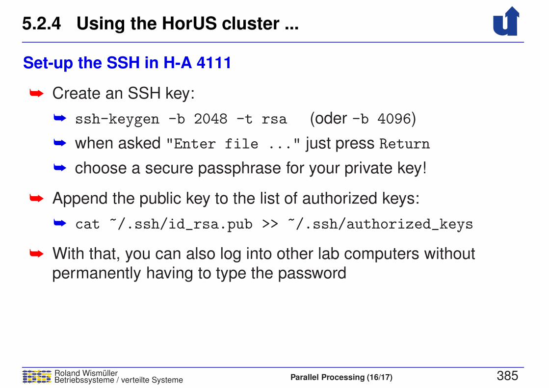
5.2.4 Using the HorUS cluster ...
Roland WismullerBetriebssysteme / verteilte Systeme Parallel Processing (16/17) 385
Set-up the SSH in H-A 4111
➥ Create an SSH key:
➥ ssh-keygen -b 2048 -t rsa (oder -b 4096)
➥ when asked "Enter file ..." just press Return
➥ choose a secure passphrase for your private key!
➥ Append the public key to the list of authorized keys:
➥ cat ~/.ssh/id_rsa.pub >> ~/.ssh/authorized_keys
➥ With that, you can also log into other lab computers without
permanently having to type the password
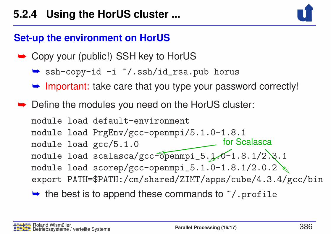
5.2.4 Using the HorUS cluster ...
Roland WismullerBetriebssysteme / verteilte Systeme Parallel Processing (16/17) 386
Set-up the environment on HorUS
➥ Copy your (public!) SSH key to HorUS
➥ ssh-copy-id -i ~/.ssh/id_rsa.pub horus
➥ Important: take care that you type your password correctly!
➥
for Scalasca
Define the modules you need on the HorUS cluster:
module load default-environment
module load PrgEnv/gcc-openmpi/5.1.0-1.8.1
module load gcc/5.1.0
module load scalasca/gcc-openmpi_5.1.0-1.8.1/2.3.1
module load scorep/gcc-openmpi_5.1.0-1.8.1/2.0.2
export PATH=$PATH:/cm/shared/ZIMT/apps/cube/4.3.4/gcc/bin
➥ the best is to append these commands to ~/.profile
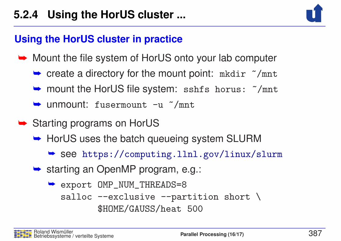
5.2.4 Using the HorUS cluster ...
Roland WismullerBetriebssysteme / verteilte Systeme Parallel Processing (16/17) 387
Using the HorUS cluster in practice
➥ Mount the file system of HorUS onto your lab computer
➥ create a directory for the mount point: mkdir ~/mnt
➥ mount the HorUS file system: sshfs horus: ~/mnt
➥ unmount: fusermount -u ~/mnt
➥ Starting programs on HorUS
➥ HorUS uses the batch queueing system SLURM
➥ see https://computing.llnl.gov/linux/slurm
➥ starting an OpenMP program, e.g.:
➥ export OMP_NUM_THREADS=8
salloc --exclusive --partition short \
$HOME/GAUSS/heat 500

Roland WismullerBetriebssysteme / verteilte Systeme Parallel Processing (17/17) xviii
Roland Wismuller
Universitat Siegen
Tel.: 0271/740-4050, Buro: H-B 8404
Stand: January 23, 2018
Parallel Processing
WS 2017/18
04.12.2017

5.3 Exercise: Sokoban Solver
Roland WismullerBetriebssysteme / verteilte Systeme Parallel Processing (17/17) 388
Background
➥ Sokoban: japanese for “warehouse keeper”
➥ Computer game, developed in 1982 by Hiroyuki Imabayashi
➥ Goal: player must push all objects (boxes) to the target positions(storage locations)
➥ boxes can only be pushed, not pulled
➥ only one box can be pushed at a time
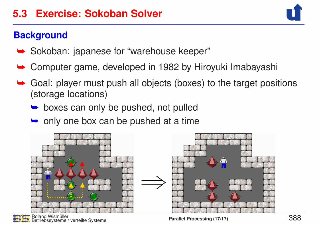
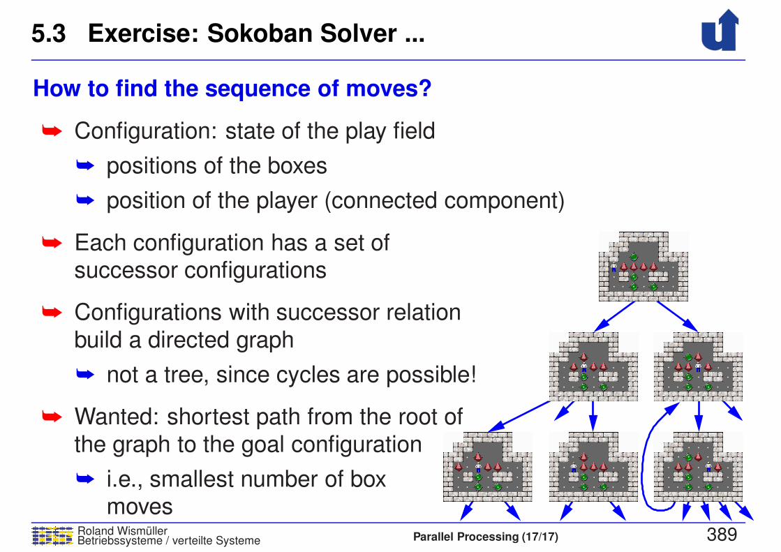
5.3 Exercise: Sokoban Solver ...
Roland WismullerBetriebssysteme / verteilte Systeme Parallel Processing (17/17) 389
How to find the sequence of moves?
➥ Configuration: state of the play field
➥ positions of the boxes
➥ position of the player (connected component)
➥ Each configuration has a set ofsuccessor configurations
➥ Configurations with successor relation
build a directed graph
➥ not a tree, since cycles are possible!
➥ Wanted: shortest path from the root of
the graph to the goal configuration
➥ i.e., smallest number of boxmoves
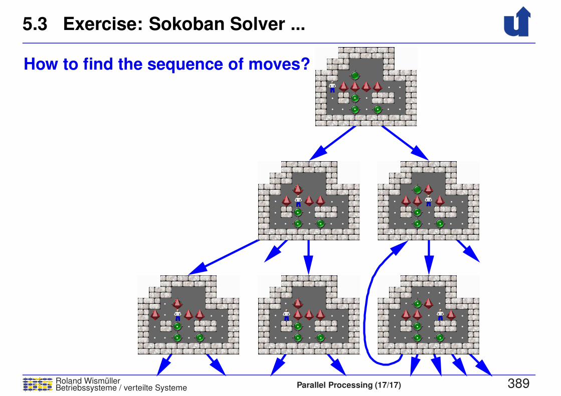
5.3 Exercise: Sokoban Solver ...
Roland WismullerBetriebssysteme / verteilte Systeme Parallel Processing (17/17) 389
How to find the sequence of moves?
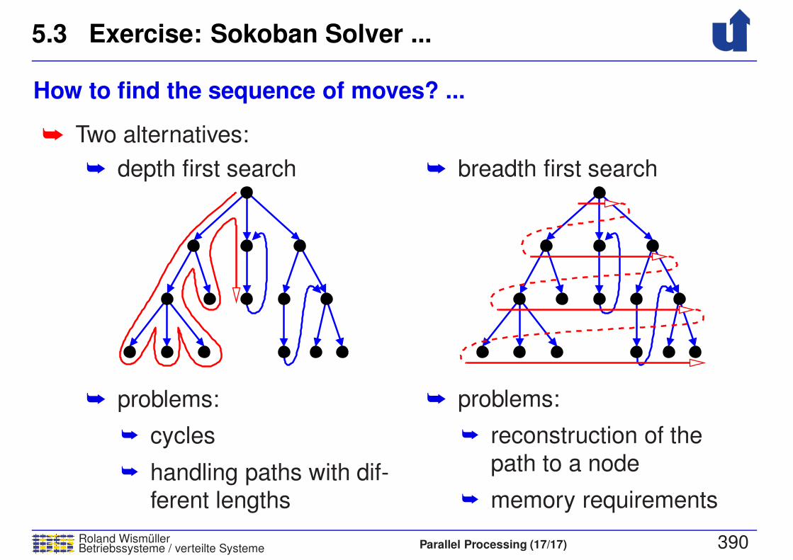
5.3 Exercise: Sokoban Solver ...
Roland WismullerBetriebssysteme / verteilte Systeme Parallel Processing (17/17) 390
How to find the sequence of moves? ...
➥ Two alternatives:
➥ depth first search
➥ problems:
➥ cycles
➥ handling paths with dif-ferent lengths
➥ breadth first search
➥ problems:
➥ reconstruction of the
path to a node
➥ memory requirements
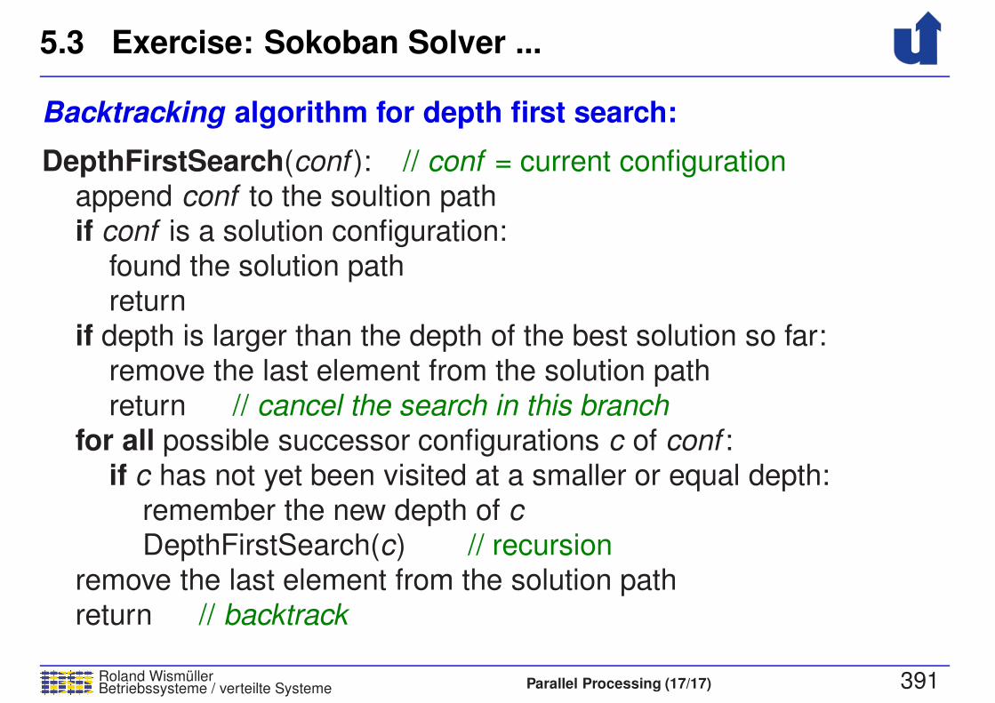
5.3 Exercise: Sokoban Solver ...
Roland WismullerBetriebssysteme / verteilte Systeme Parallel Processing (17/17) 391
Backtracking algorithm for depth first search:
DepthFirstSearch(conf ): // conf = current configurationappend conf to the soultion pathif conf is a solution configuration:
found the solution pathreturn
if depth is larger than the depth of the best solution so far:remove the last element from the solution pathreturn // cancel the search in this branch
for all possible successor configurations c of conf :if c has not yet been visited at a smaller or equal depth:
remember the new depth of cDepthFirstSearch(c) // recursion
remove the last element from the solution pathreturn // backtrack
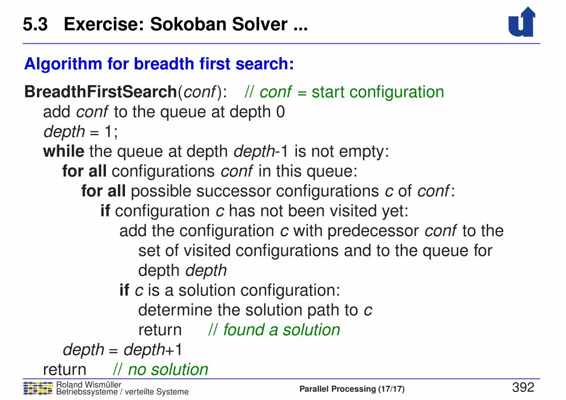
5.3 Exercise: Sokoban Solver ...
Roland WismullerBetriebssysteme / verteilte Systeme Parallel Processing (17/17) 392
Algorithm for breadth first search:
BreadthFirstSearch(conf ): // conf = start configurationadd conf to the queue at depth 0depth = 1;while the queue at depth depth-1 is not empty:
for all configurations conf in this queue:for all possible successor configurations c of conf :
if configuration c has not been visited yet:add the configuration c with predecessor conf to the
set of visited configurations and to the queue fordepth depth
if c is a solution configuration:determine the solution path to creturn // found a solution
depth = depth+1return // no solution
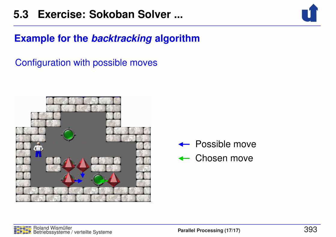
5.3 Exercise: Sokoban Solver ...
Roland WismullerBetriebssysteme / verteilte Systeme Parallel Processing (17/17) 393
Example for the backtracking algorithm
Possible move
Chosen move
Configuration with possible moves
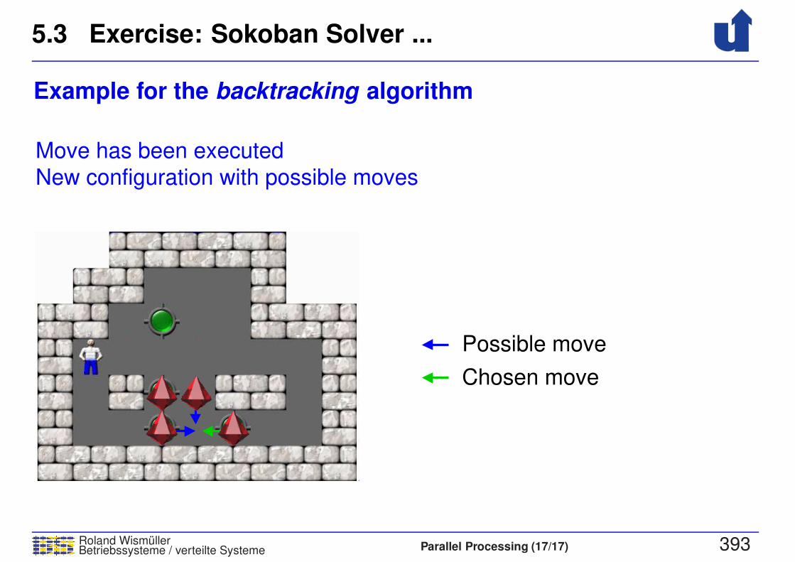
5.3 Exercise: Sokoban Solver ...
Roland WismullerBetriebssysteme / verteilte Systeme Parallel Processing (17/17) 393
Example for the backtracking algorithm
Possible move
Chosen move
New configuration with possible movesMove has been executed
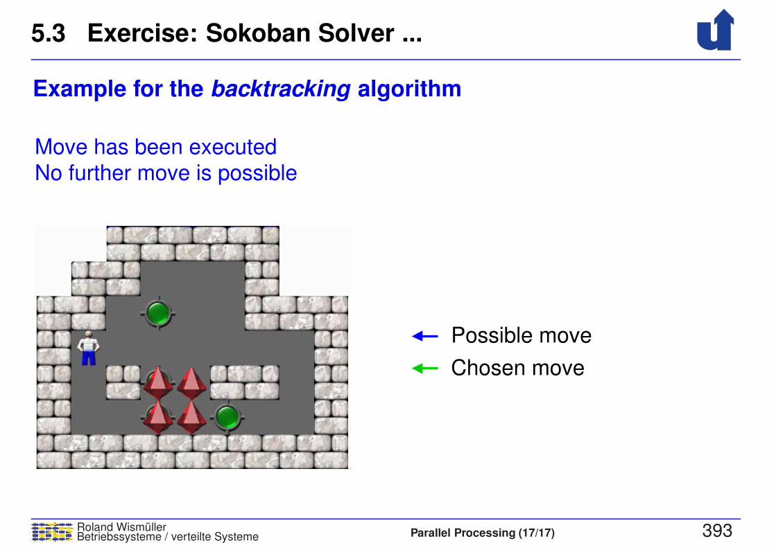
5.3 Exercise: Sokoban Solver ...
Roland WismullerBetriebssysteme / verteilte Systeme Parallel Processing (17/17) 393
Example for the backtracking algorithm
Possible move
Chosen move
Move has been executedNo further move is possible
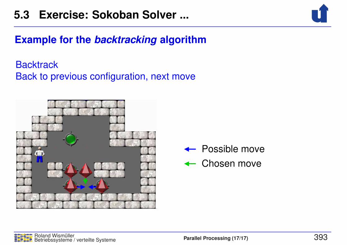
5.3 Exercise: Sokoban Solver ...
Roland WismullerBetriebssysteme / verteilte Systeme Parallel Processing (17/17) 393
Example for the backtracking algorithm
Possible move
Chosen move
BacktrackBack to previous configuration, next move

Roland WismullerBetriebssysteme / verteilte Systeme Parallel Processing (17/17) xix
Roland Wismuller
Universitat Siegen
Tel.: 0271/740-4050, Buro: H-B 8404
Stand: January 23, 2018
Parallel Processing
WS 2017/18
15.01.2018
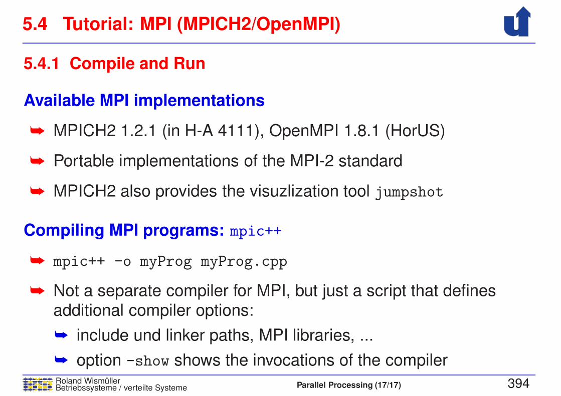
5.4 Tutorial: MPI (MPICH2/OpenMPI)
Roland WismullerBetriebssysteme / verteilte Systeme Parallel Processing (17/17) 394
5.4.1 Compile and Run
Available MPI implementations
➥ MPICH2 1.2.1 (in H-A 4111), OpenMPI 1.8.1 (HorUS)
➥ Portable implementations of the MPI-2 standard
➥ MPICH2 also provides the visuzlization tool jumpshot
Compiling MPI programs: mpic++
➥ mpic++ -o myProg myProg.cpp
➥ Not a separate compiler for MPI, but just a script that definesadditional compiler options:
➥ include und linker paths, MPI libraries, ...
➥ option -show shows the invocations of the compiler
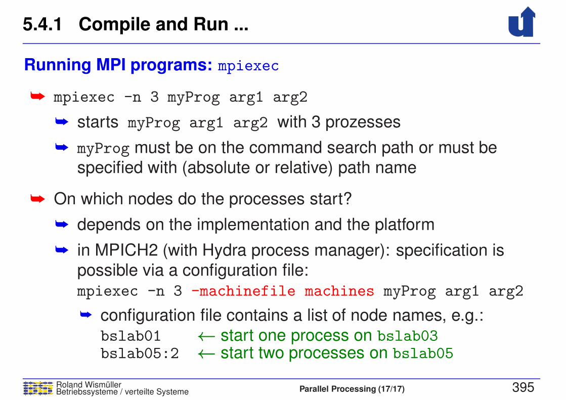
5.4.1 Compile and Run ...
Roland WismullerBetriebssysteme / verteilte Systeme Parallel Processing (17/17) 395
Running MPI programs: mpiexec
➥ mpiexec -n 3 myProg arg1 arg2
➥ starts myProg arg1 arg2 with 3 prozesses
➥ myProg must be on the command search path or must be
specified with (absolute or relative) path name
➥ On which nodes do the processes start?
➥ depends on the implementation and the platform
➥ in MPICH2 (with Hydra process manager): specification is
possible via a configuration file:
mpiexec -n 3 -machinefile machines myProg arg1 arg2
➥ configuration file contains a list of node names, e.g.:
bslab01 ← start one process on bslab03bslab05:2 ← start two processes on bslab05
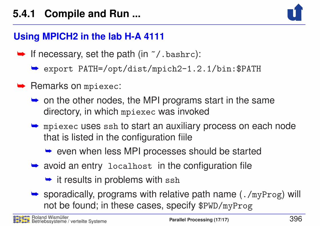
5.4.1 Compile and Run ...
Roland WismullerBetriebssysteme / verteilte Systeme Parallel Processing (17/17) 396
Using MPICH2 in the lab H-A 4111
➥ If necessary, set the path (in ~/.bashrc):
➥ export PATH=/opt/dist/mpich2-1.2.1/bin:$PATH
➥ Remarks on mpiexec:
➥ on the other nodes, the MPI programs start in the samedirectory, in which mpiexec was invoked
➥ mpiexec uses ssh to start an auxiliary process on each node
that is listed in the configuration fiile
➥ even when less MPI processes should be started
➥ avoid an entry localhost in the configuration file
➥ it results in problems with ssh
➥ sporadically, programs with relative path name (./myProg) willnot be found; in these cases, specify $PWD/myProg
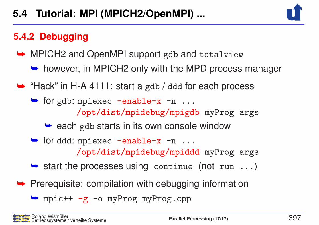
5.4 Tutorial: MPI (MPICH2/OpenMPI) ...
Roland WismullerBetriebssysteme / verteilte Systeme Parallel Processing (17/17) 397
5.4.2 Debugging
➥ MPICH2 and OpenMPI support gdb and totalview
➥ however, in MPICH2 only with the MPD process manager
➥ “Hack” in H-A 4111: start a gdb / ddd for each process
➥ for gdb: mpiexec -enable-x -n ...
/opt/dist/mpidebug/mpigdb myProg args
➥ each gdb starts in its own console window
➥ for ddd: mpiexec -enable-x -n ...
/opt/dist/mpidebug/mpiddd myProg args
➥ start the processes using continue (not run ...)
➥ Prerequisite: compilation with debugging information
➥ mpic++ -g -o myProg myProg.cpp

5.4 Tutorial: MPI (MPICH2/OpenMPI) ...
Roland WismullerBetriebssysteme / verteilte Systeme Parallel Processing (17/17) 398
5.4.3 Performance Analysis using Scalasca
➥ In principle, in the same way as for OpenMP
➥ Compiling the program:
➥ scalasca -instrument mpic++ -o myprog myprog.cpp
➥ Running the programms:
➥ scalasca -analyze mpiexec -n 4 ... ./myprog
➥ creates a directory scorep myprog 4 sum
➥ 4 indicates the number of processes
➥ directory must not previously exist; delete it, if necessary
➥ Interactive analysis of the recorded data:
➥ scalasca -examine scorep myprog 4 sum
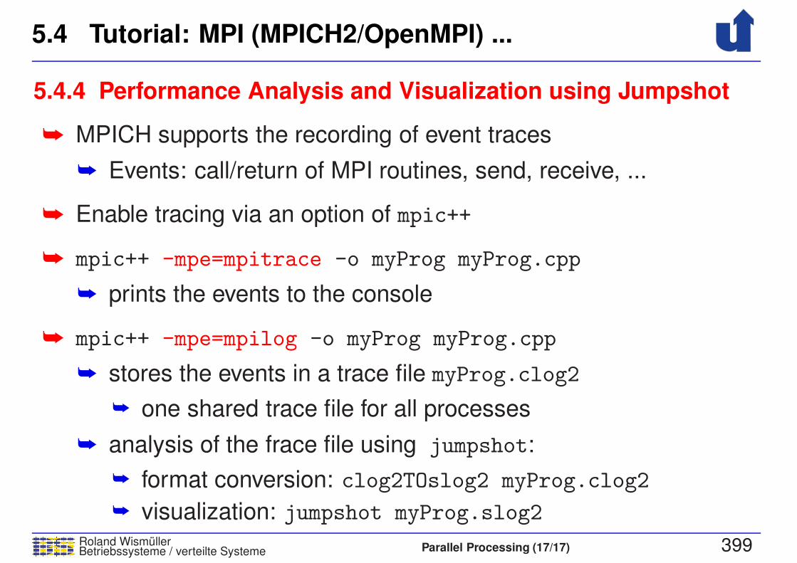
5.4 Tutorial: MPI (MPICH2/OpenMPI) ...
Roland WismullerBetriebssysteme / verteilte Systeme Parallel Processing (17/17) 399
5.4.4 Performance Analysis and Visualization using Jumpshot
➥ MPICH supports the recording of event traces
➥ Events: call/return of MPI routines, send, receive, ...
➥ Enable tracing via an option of mpic++
➥ mpic++ -mpe=mpitrace -o myProg myProg.cpp
➥ prints the events to the console
➥ mpic++ -mpe=mpilog -o myProg myProg.cpp
➥ stores the events in a trace file myProg.clog2
➥ one shared trace file for all processes
➥ analysis of the frace file using jumpshot:
➥ format conversion: clog2TOslog2 myProg.clog2
➥ visualization: jumpshot myProg.slog2
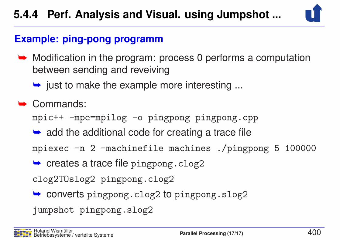
5.4.4 Perf. Analysis and Visual. using Jumpshot ...
Roland WismullerBetriebssysteme / verteilte Systeme Parallel Processing (17/17) 400
Example: ping-pong programm
➥ Modification in the program: process 0 performs a computation
between sending and reveiving
➥ just to make the example more interesting ...
➥ Commands:
mpic++ -mpe=mpilog -o pingpong pingpong.cpp
➥ add the additional code for creating a trace file
mpiexec -n 2 -machinefile machines ./pingpong 5 100000
➥ creates a trace file pingpong.clog2
clog2TOslog2 pingpong.clog2
➥ converts pingpong.clog2 to pingpong.slog2
jumpshot pingpong.slog2
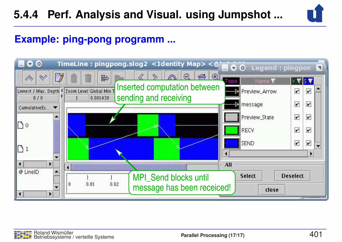
5.4.4 Perf. Analysis and Visual. using Jumpshot ...
Roland WismullerBetriebssysteme / verteilte Systeme Parallel Processing (17/17) 401
Example: ping-pong programm ...
Inserted computation betweensending and receiving
MPI_Send blocks untilmessage has been receiced!
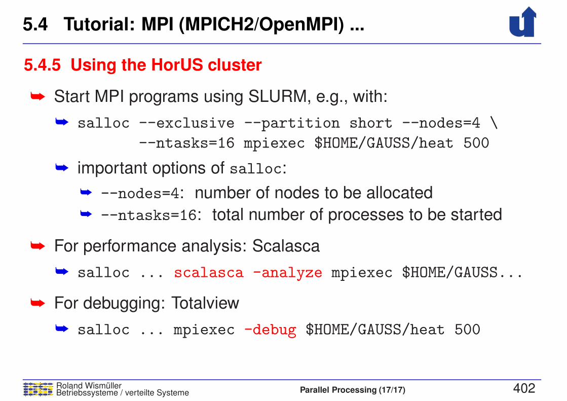
5.4 Tutorial: MPI (MPICH2/OpenMPI) ...
Roland WismullerBetriebssysteme / verteilte Systeme Parallel Processing (17/17) 402
5.4.5 Using the HorUS cluster
➥ Start MPI programs using SLURM, e.g., with:
➥ salloc --exclusive --partition short --nodes=4 \
--ntasks=16 mpiexec $HOME/GAUSS/heat 500
➥ important options of salloc:
➥ --nodes=4: number of nodes to be allocated
➥ --ntasks=16: total number of processes to be started
➥ For performance analysis: Scalasca
➥ salloc ... scalasca -analyze mpiexec $HOME/GAUSS...
➥ For debugging: Totalview
➥ salloc ... mpiexec -debug $HOME/GAUSS/heat 500

5.5 Exercise: Jacobi and Gauss/Seidel with MPI
Roland WismullerBetriebssysteme / verteilte Systeme Parallel Processing (17/17) 403
Gerneral approach
0. Matrix with temperature values
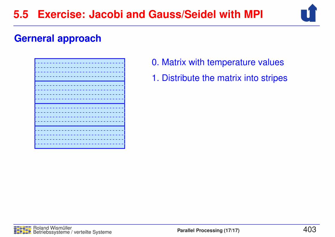
5.5 Exercise: Jacobi and Gauss/Seidel with MPI
Roland WismullerBetriebssysteme / verteilte Systeme Parallel Processing (17/17) 403
Gerneral approach
1. Distribute the matrix into stripes
0. Matrix with temperature values
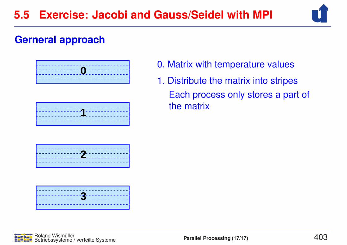
5.5 Exercise: Jacobi and Gauss/Seidel with MPI
Roland WismullerBetriebssysteme / verteilte Systeme Parallel Processing (17/17) 403
Gerneral approach
the matrix
Each process only stores a part of
2
3
1
01. Distribute the matrix into stripes
0. Matrix with temperature values
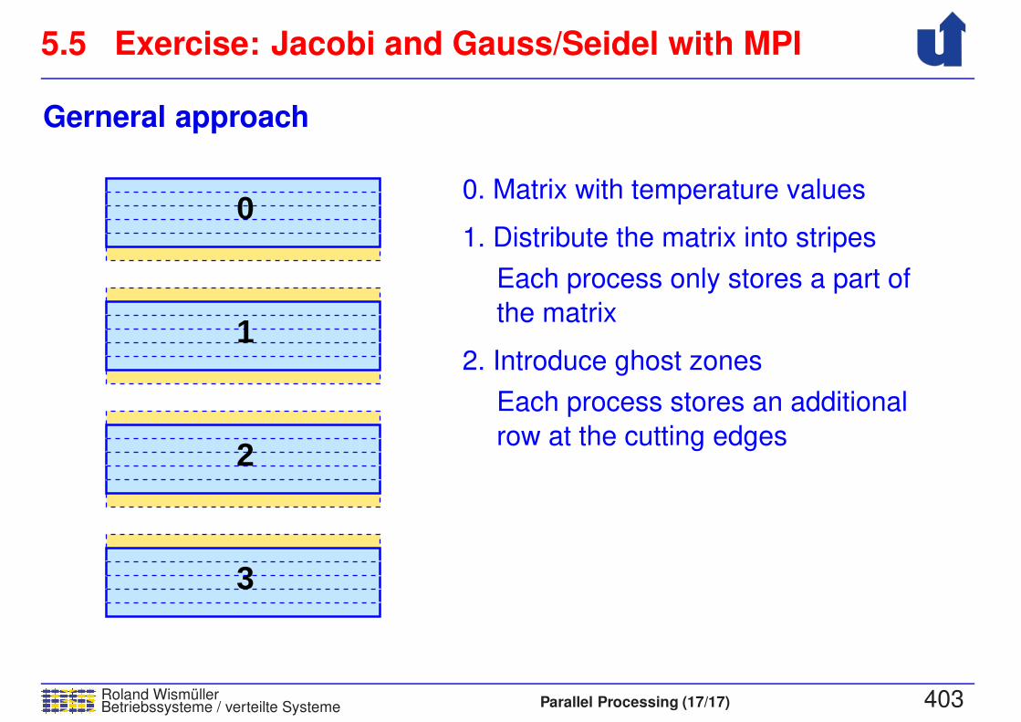
5.5 Exercise: Jacobi and Gauss/Seidel with MPI
Roland WismullerBetriebssysteme / verteilte Systeme Parallel Processing (17/17) 403
Gerneral approach
row at the cutting edges
Each process stores an additional
2. Introduce ghost zones
the matrix
Each process only stores a part of
2
3
1
01. Distribute the matrix into stripes
0. Matrix with temperature values
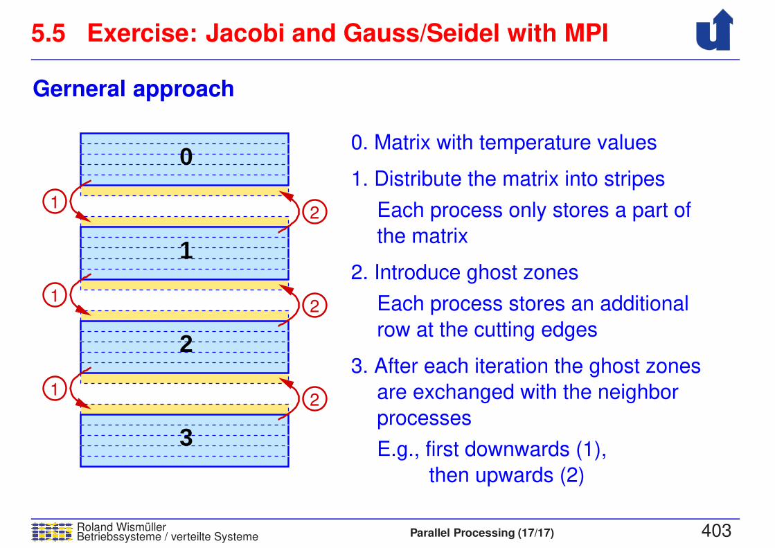
5.5 Exercise: Jacobi and Gauss/Seidel with MPI
Roland WismullerBetriebssysteme / verteilte Systeme Parallel Processing (17/17) 403
Gerneral approach
row at the cutting edges
Each process stores an additional
2. Introduce ghost zones
the matrix
Each process only stores a part of
2
3
1
01. Distribute the matrix into stripes
0. Matrix with temperature values
1
1
12
2
2
processes
are exchanged with the neighbor
3. After each iteration the ghost zones
E.g., first downwards (1),
then upwards (2)
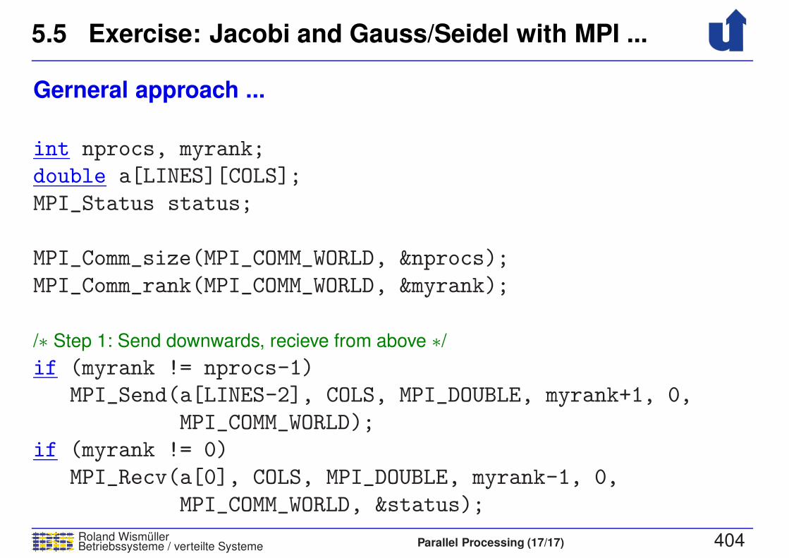
5.5 Exercise: Jacobi and Gauss/Seidel with MPI ...
Roland WismullerBetriebssysteme / verteilte Systeme Parallel Processing (17/17) 404
Gerneral approach ...
int nprocs, myrank;
double a[LINES][COLS];
MPI_Status status;
MPI_Comm_size(MPI_COMM_WORLD, &nprocs);
MPI_Comm_rank(MPI_COMM_WORLD, &myrank);
/∗ Step 1: Send downwards, recieve from above ∗/
if (myrank != nprocs-1)
MPI_Send(a[LINES-2], COLS, MPI_DOUBLE, myrank+1, 0,
MPI_COMM_WORLD);
if (myrank != 0)
MPI_Recv(a[0], COLS, MPI_DOUBLE, myrank-1, 0,
MPI_COMM_WORLD, &status);

5.5 Exercise: Jacobi and Gauss/Seidel with MPI ...
Roland WismullerBetriebssysteme / verteilte Systeme Parallel Processing (17/17) 405
Distribution of data
➥ Close formula for the uniform distribution of an array of length n to
np processes:
➥ start(p) = n÷ np · p + max(p− (np− n mod np), 0)
➥ size(p) = (n + p)÷ np
➥ process p receives size(p) elements starting at index start(p)
➥ This results in the following index transformation:
➥ tolocal(i) = (p, i− start(p))mit p ∈ [0, np− 1] so, daß 0 ≤ i− start(p) < size(p)
➥ toglobal(p, i) = i + start(p)
➥ In addition, you have to consider the ghost zones for Jacobi and
Gauss/Seidel!
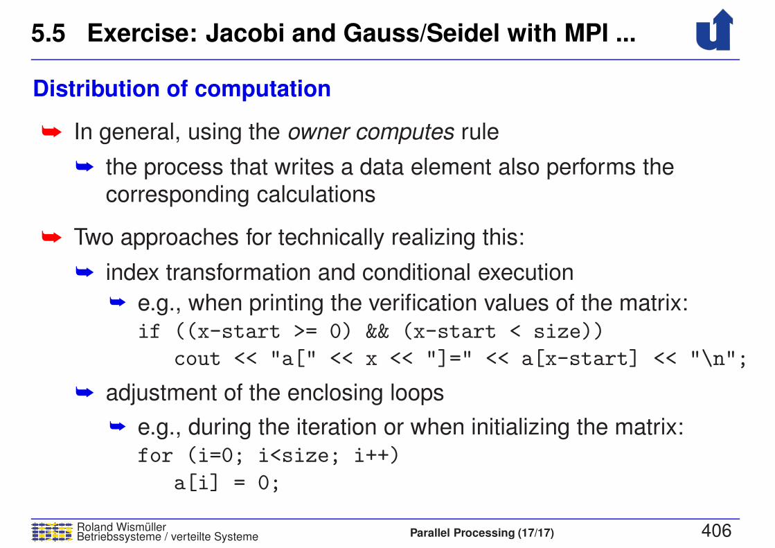
5.5 Exercise: Jacobi and Gauss/Seidel with MPI ...
Roland WismullerBetriebssysteme / verteilte Systeme Parallel Processing (17/17) 406
Distribution of computation
➥ In general, using the owner computes rule
➥ the process that writes a data element also performs the
corresponding calculations
➥ Two approaches for technically realizing this:
➥ index transformation and conditional execution
➥ e.g., when printing the verification values of the matrix:
if ((x-start >= 0) && (x-start < size))
cout << "a[" << x << "]=" << a[x-start] << "\n";
➥ adjustment of the enclosing loops
➥ e.g., during the iteration or when initializing the matrix:
for (i=0; i<size; i++)
a[i] = 0;
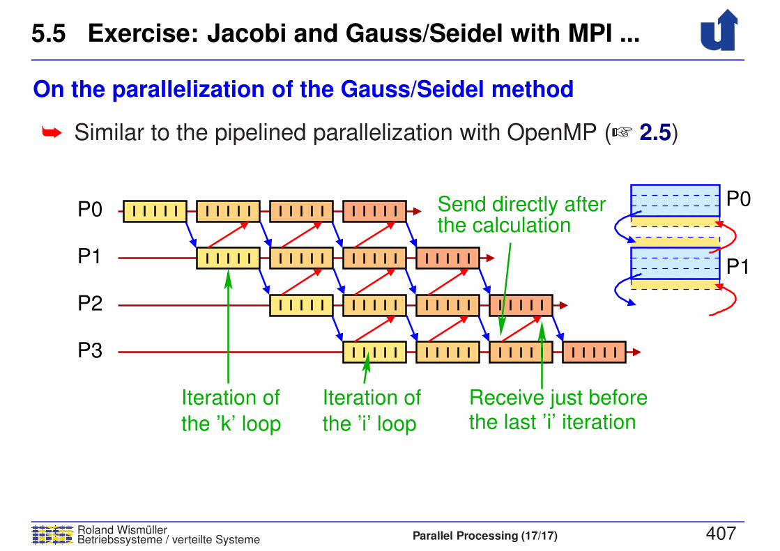
5.5 Exercise: Jacobi and Gauss/Seidel with MPI ...
Roland WismullerBetriebssysteme / verteilte Systeme Parallel Processing (17/17) 407
On the parallelization of the Gauss/Seidel method
➥ Similar to the pipelined parallelization with OpenMP (☞ 2.5)
P2
P3
P1
P0P0
P1
Iteration of
the ’i’ loop
Iteration of
the ’k’ loop
Receive just beforethe last ’i’ iteration
the calculationSend directly after

5.5 Exercise: Jacobi and Gauss/Seidel with MPI ...
Roland WismullerBetriebssysteme / verteilte Systeme Parallel Processing (17/17) 408
Obtained speedup for different matrix sizes
XEON clusterblockwisedistribution
Jacobi 8000Jacobi 4000
Jacobi 2000
Jacobi 1000
Jacobi 500
ideal
Speedup
Processors
0
2
4
6
8
10
12
14
16
2 4 6 8 10 12 14 16
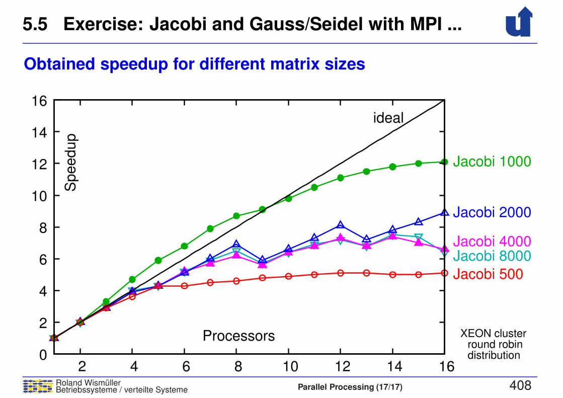
5.5 Exercise: Jacobi and Gauss/Seidel with MPI ...
Roland WismullerBetriebssysteme / verteilte Systeme Parallel Processing (17/17) 408
Obtained speedup for different matrix sizes
XEON clusterround robindistribution
Jacobi 8000Jacobi 4000
Jacobi 2000
Jacobi 1000
Jacobi 500
ideal
Speedup
Processors
0
2
4
6
8
10
12
14
16
2 4 6 8 10 12 14 16
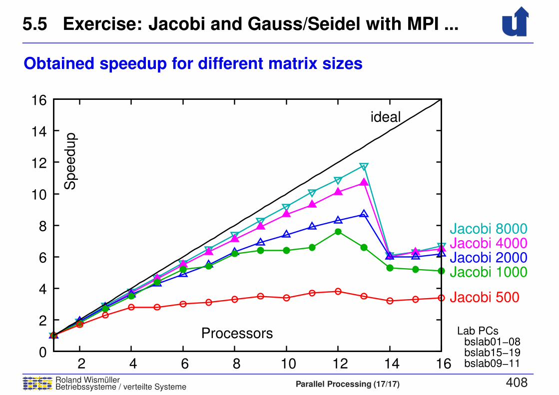
5.5 Exercise: Jacobi and Gauss/Seidel with MPI ...
Roland WismullerBetriebssysteme / verteilte Systeme Parallel Processing (17/17) 408
Obtained speedup for different matrix sizes
Jacobi 8000Jacobi 4000Jacobi 2000Jacobi 1000
Jacobi 500
Lab PCsbslab01−08bslab15−19bslab09−11
ideal
Speedup
Processors
0
2
4
6
8
10
12
14
16
2 4 6 8 10 12 14 16
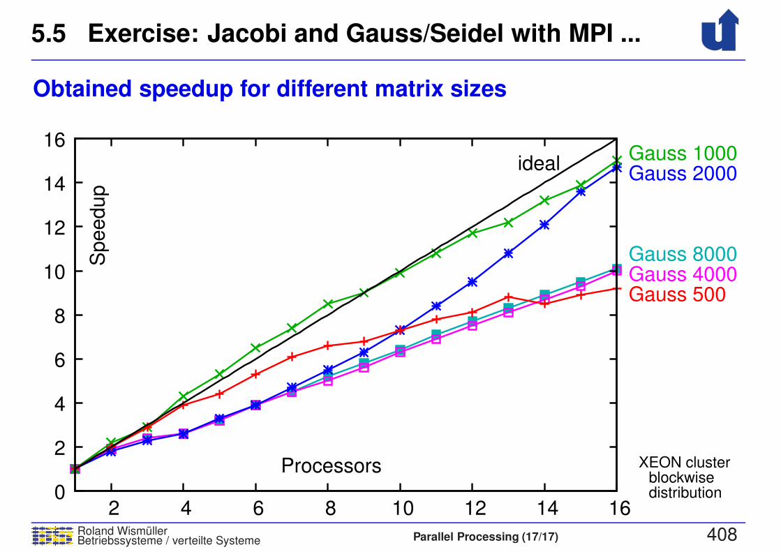
5.5 Exercise: Jacobi and Gauss/Seidel with MPI ...
Roland WismullerBetriebssysteme / verteilte Systeme Parallel Processing (17/17) 408
Obtained speedup for different matrix sizes
XEON clusterblockwisedistribution
Gauss 8000Gauss 4000
Gauss 2000Gauss 1000
Gauss 500
ideal
Sp
ee
du
p
Processors
0
2
4
6
8
10
12
14
16
2 4 6 8 10 12 14 16

5.5 Exercise: Jacobi and Gauss/Seidel with MPI ...
Roland WismullerBetriebssysteme / verteilte Systeme Parallel Processing (17/17) 408
Obtained speedup for different matrix sizes
XEON clusterround robindistribution
Gauss 8000
Gauss 4000
Gauss 2000Gauss 1000
Gauss 500
ideal
Sp
ee
du
p
Processors
0
2
4
6
8
10
12
14
16
2 4 6 8 10 12 14 16
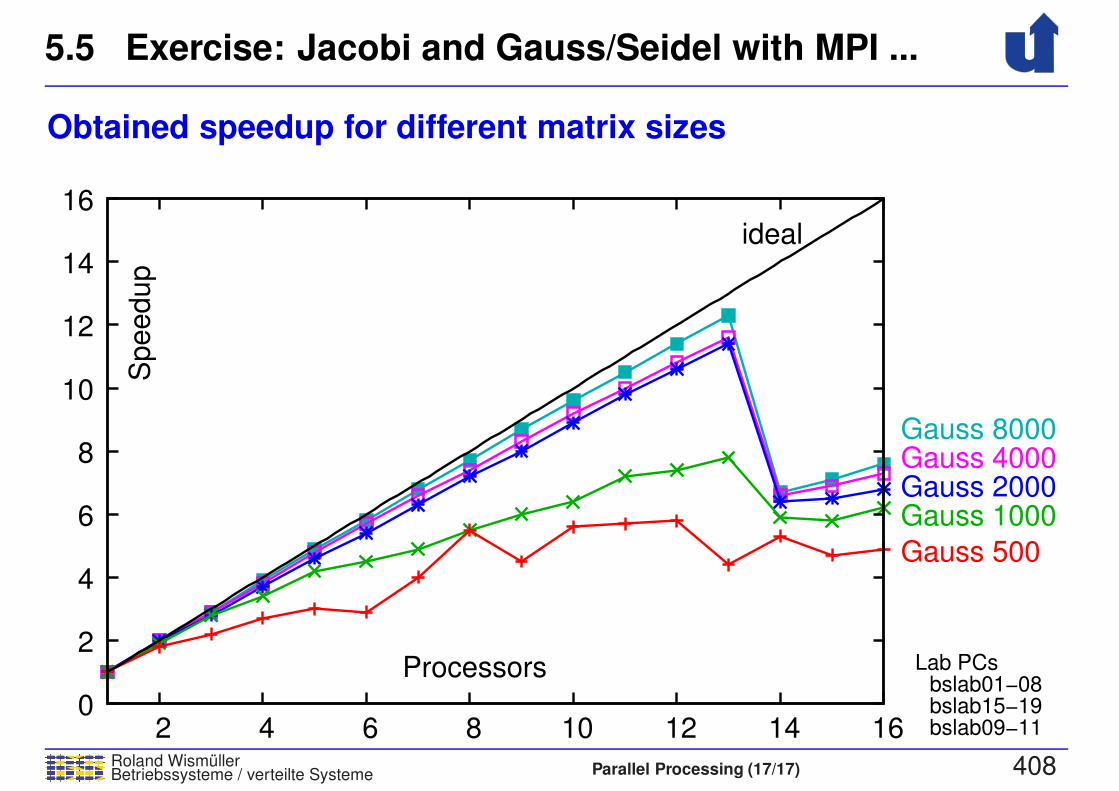
5.5 Exercise: Jacobi and Gauss/Seidel with MPI ...
Roland WismullerBetriebssysteme / verteilte Systeme Parallel Processing (17/17) 408
Obtained speedup for different matrix sizes
Gauss 8000Gauss 4000Gauss 2000Gauss 1000
Gauss 500
Lab PCsbslab01−08bslab15−19bslab09−11
ideal
Sp
ee
du
p
Processors
0
2
4
6
8
10
12
14
16
2 4 6 8 10 12 14 16
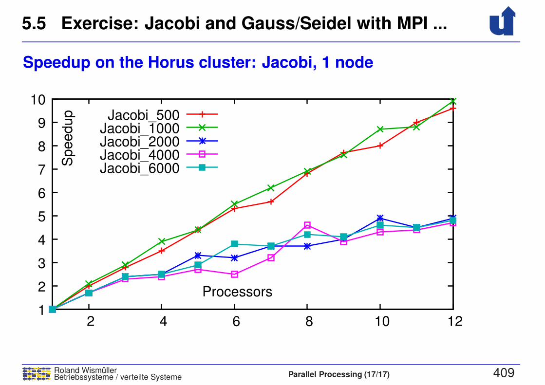
5.5 Exercise: Jacobi and Gauss/Seidel with MPI ...
Roland WismullerBetriebssysteme / verteilte Systeme Parallel Processing (17/17) 409
Speedup on the Horus cluster: Jacobi, 1 node
Processors
Sp
ee
du
p Jacobi_500Jacobi_1000Jacobi_2000Jacobi_4000Jacobi_6000
1
2
3
4
5
6
7
8
9
10
2 4 6 8 10 12
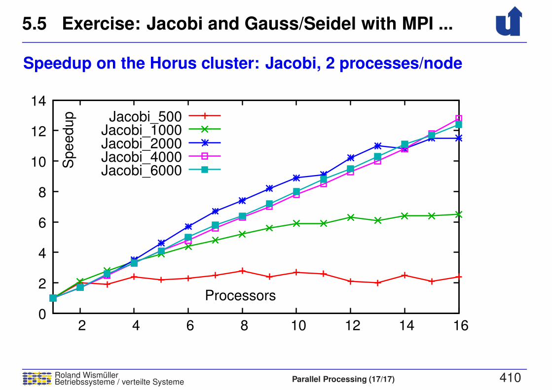
5.5 Exercise: Jacobi and Gauss/Seidel with MPI ...
Roland WismullerBetriebssysteme / verteilte Systeme Parallel Processing (17/17) 410
Speedup on the Horus cluster: Jacobi, 2 processes/node
Processors
Sp
ee
du
p Jacobi_500Jacobi_1000Jacobi_2000Jacobi_4000Jacobi_6000
0
2
4
6
8
10
12
14
2 4 6 8 10 12 14 16
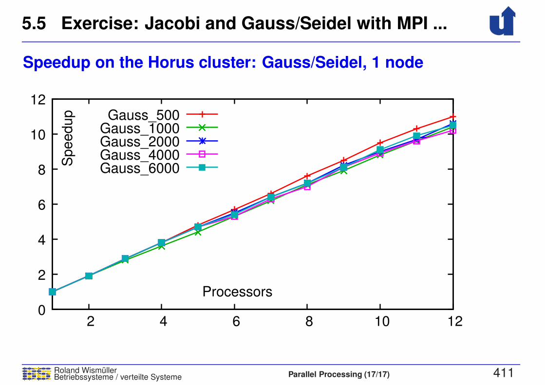
5.5 Exercise: Jacobi and Gauss/Seidel with MPI ...
Roland WismullerBetriebssysteme / verteilte Systeme Parallel Processing (17/17) 411
Speedup on the Horus cluster: Gauss/Seidel, 1 node
Processors
Sp
ee
du
p Gauss_500Gauss_1000Gauss_2000Gauss_4000Gauss_6000
0
2
4
6
8
10
12
2 4 6 8 10 12
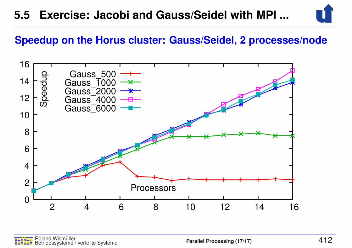
5.5 Exercise: Jacobi and Gauss/Seidel with MPI ...
Roland WismullerBetriebssysteme / verteilte Systeme Parallel Processing (17/17) 412
Speedup on the Horus cluster: Gauss/Seidel, 2 processes/node
Processors
Sp
ee
du
p Gauss_500Gauss_1000Gauss_2000Gauss_4000Gauss_6000
0
2
4
6
8
10
12
14
16
2 4 6 8 10 12 14 16