Parallel Multigrid Solver for Large Sparse Linear Systems (08378)_Project... · Parallel Multigrid...

Parallel Multigrid Solver for Large Sparse LinearSystems

A PROJECT REPORT

SUBMITTED IN PARTIAL FULFILMENT OF THE

REQUIREMENTS FOR THE DEGREE OF

Master of Technology

IN

Computational Science

by

Shiladitya Banerjee

Supercomputer Education and Research Centre

Indian Institute of Science

BANGALORE – 560 012

JUNE 2013

1

c©Shiladitya Banerjee

JUNE 2013All rights reserved

i

Dedicated to my Parents

Acknowledgements

It would not have been possible to write this thesis without the help and support of the kind

people around me, to only some of whom it is possible to give particular mention here.

First I would like to thank my project guide, Dr. Sashikumaar Ganesan, without whose support

and patience this thesis would not have been possible. Under his guidance not only have I

completed my project work, but have also learnt much which will be of immense help to me

in my future academic and professional life.

I thank the reviewer for his constructive and helpful suggestions.

The library facilities and computer facilities of the Institute have been indispensable.

I would also like to thank all my classmates (Nilesh, Sai, Hari, Ankit, Anurag, Vivek, Siva,

Sanjeev) and colleagues (Calvin, JP, Kalyan, Milind, Vishal) for their invaluable advice and

support throughout the course. I will always cherish their friendship.

Last but not the least, I would like to express my sincere gratitude to all those who have directly

or indirectly helped in making this happen.

ii

Abstract

The aim of this work is to develop an efficient and robust parallel (MPI) Multigrid algorithm

for solving PDEs using Metis/ParMetis package for parallel Multigrid solvers. This work also

involves the implementation of parallel data structures for conforming, nonconforming and

discontinuous finite element spaces on a hierarchy of partitioned mesh. The efficiency and the

robustness of the algorithm have been tested with a set of examples.

iii

Contents

Acknowledgements ii

Abstract iii

1 Introduction 1

1.1 Large scale problems and their computational need . . . . . . . . . . . . . . 1

1.2 High Performance Computing . . . . . . . . . . . . . . . . . . . . . . . . . 2

1.3 Parallel Systems . . . . . . . . . . . . . . . . . . . . . . . . . . . . . . . . . 2

1.4 Message Passing Interface (MPI) . . . . . . . . . . . . . . . . . . . . . . . . 2

1.5 Outline of the Thesis . . . . . . . . . . . . . . . . . . . . . . . . . . . . . . 3

2 The Finite Element Method (FEM) 4

3 Domain Decomposition and Parallel Implementation 11

3.1 ParMooN . . . . . . . . . . . . . . . . . . . . . . . . . . . . . . . . . . . . 11

3.2 Domain Decomposition . . . . . . . . . . . . . . . . . . . . . . . . . . . . . 11

3.3 FE Communicator . . . . . . . . . . . . . . . . . . . . . . . . . . . . . . . . 13

3.4 Solving the System of Equations using Parallel Iterative Solver . . . . . . . . 15

4 Multigrid Solver 19

4.1 The Restriction and Prolongation Operators . . . . . . . . . . . . . . . . . . 20

4.2 Computational Complexity . . . . . . . . . . . . . . . . . . . . . . . . . . . 21

iv

CONTENTS v

5 Implementation of Multigrid Solver in ParMooN 22

5.1 Creation of Hierarchy of Meshes in Parallel . . . . . . . . . . . . . . . . . . 22

5.2 Components of a Multigrid Level . . . . . . . . . . . . . . . . . . . . . . . . 22

5.3 Mapping Strategy in Parallel . . . . . . . . . . . . . . . . . . . . . . . . . . 23

5.4 Parallel Multigrid V-Cycle . . . . . . . . . . . . . . . . . . . . . . . . . . . 24

6 Results and Conclusion 28

6.1 Sequential and Parallel Results . . . . . . . . . . . . . . . . . . . . . . . . . 28

6.2 Parallel Multigrid experiments . . . . . . . . . . . . . . . . . . . . . . . . . 29

Bibliography 34

List of Figures

2.1 Domain with Dirichlet and Neumann boundary conditions . . . . . . . . . . 5

2.2 Triangulation of Domain . . . . . . . . . . . . . . . . . . . . . . . . . . . . 7

2.3 Conforming, Non-Conforming and Discontinuous Finite Elements (left to right) 8

2.4 Basis Function at the Boundary and in the Interior . . . . . . . . . . . . . . . 8

2.5 Assembling the system matrix . . . . . . . . . . . . . . . . . . . . . . . . . 10

3.1 Support of basis functions associated with a Degree of Freedom on the vertex,

edge and interior of the element . . . . . . . . . . . . . . . . . . . . . . . . 12

3.2 Mesh partition using METIS : The green colored cells denote the Halo Cells

and the red colored cells denote the Dependent Cells . . . . . . . . . . . . . 13

3.3 Flowchart describing Algorithm 1 for Parallel Code . . . . . . . . . . . . . . 17

3.4 Flowchart describing Algorithm 2 for FE Communicator . . . . . . . . . . . 18

4.1 Two Grid and Multigrid V-cycle . . . . . . . . . . . . . . . . . . . . . . . . 20

5.1 Part I: Initialization of domain in each processor . . . . . . . . . . . . . . . . 26

5.2 Part II: Construction of Multigrid Levels . . . . . . . . . . . . . . . . . . . . 26

5.3 Flowchart for Parallel Multigrid V-Cycle . . . . . . . . . . . . . . . . . . . . 27

6.1 Sequential Solution along with Parallel solution in all 4 processors . . . . . . 29

6.2 Speedup vs Number of processors (Linear Conforming Finite Elements) . . . 30

6.3 Speedup vs Grid Size (Linear Conforming Finite Elements) . . . . . . . . . . 31

6.4 Speedup vs Number of processors (Quadratic Conforming Finite Elements) . 31

6.5 Speedup vs Grid Size (Quadratic Conforming Finite Elements) . . . . . . . . 31

vi

LIST OF FIGURES vii

6.6 Speedup vs Number of processors (Quadratic Conforming Finite Elements) . 32

6.7 Scalability Measure for 32 Processors . . . . . . . . . . . . . . . . . . . . . 32

Chapter 1

Introduction

1.1 Large scale problems and their computational need

Today there is an urgent need to solve many real-world computationally intensive problems

faster. In fields like astrophysics, climate modelling and fluid flows many such examples are

found. All real world phenomena can be described by Partial Differential Equations. For

example the NavierStokes equations may be used to model the weather, ocean currents, water

flow in a pipe and air flow around a wing. The Navier−Stokes equation for incompressible

flows can be written as follows :

∂u

∂t+ u · ∇u +∇p =

1

Re4u+ f

∇ · u = 0

There are various numerical methods available to solve these PDEs, for example , the Finite

Volume Methods (FVM), the Finite Element Method (FEM), etc. The biggest advantage of

using FEM over other numerical methods lies in its ability to handle complex geometries.

Application of these methods to a large scale problem produces a large algebraic system of

equations. Hence we need to develop efficient solvers for these large algebraic system of

equations.

1

CHAPTER 1. INTRODUCTION 2

1.2 High Performance Computing

Numerical methods and algorithms for solving large scale problems need to be efficient, scal-

able and portable. Many such large scale problems are found in the field of Computational

Fluid Dynamics (CFD). Advanced finite element simulations require parallel algorithms to

scale on clusters with thousands or tens of thousands of processor cores. Even though peta

flop parallel machines are accessible nowadays, hardware alone cannot achieve this perfor-

mance in practical problems. Hence there is a need to develop robust and efficient algorithms.

1.3 Parallel Systems

Distributed memory refers to a multiple-processor computer system in which each processor

has its own private memory. Computational tasks can only operate on local data, and if remote

data is required, the computational task must communicate with one or more remote proces-

sors. In contrast, a shared memory multi processor offers a single memory space used by all

processors. Processors do not have to be aware where data resides, except that there may be

performance penalties, and that race conditions are to be avoided.

1.4 Message Passing Interface (MPI)

Message Passing Interface (MPI) is a standardized and portable message-passing system de-

signed to function on a wide variety of distributed memory parallel computers. MPI is a

language-independent communications protocol used to program parallel computers.

As the data involved in the large scale CFD problems is enormous, it is necessary to distribute

the data among different nodes to handle the memory requirement. Hence there is a need to

develop efficient algorithms for parallelization across nodes. Keeping in mind the requirement

of a distributed memory architecture MPI [4] is the best choice.

CHAPTER 1. INTRODUCTION 3

1.5 Outline of the Thesis

In chapter 2 we present an introduction to the Finite Element Method. Later we discuss the

domain decomposition strategy and parallel implementation of FEM in ParMooN (in-house Fi-

nite Element package). In chapter 4 we provide a brief introduction to the Multigrid Methods

followed by chapter 5, providing implementation details of the parallel multigrid solver devel-

oped. We conclude with the results achieved by implementing the parallel multigrid solver on

distributed memory systems for computationally intensive examples.

Chapter 2

The Finite Element Method (FEM)

The Finite Element Method (FEM) is a numerical technique for finding approximate solutions

to boundary value problems. It uses variational methods (the calculus of variations) to mini-

mize an error function and produce a stable solution. The subdivision of a whole domain into

simpler parts has several advantages:

• Accurate representation of complex geometry

• Inclusion of dissimilar material properties

• Easy representation of the total solution

• Capture of local effects

A typical work out of the method involves dividing the domain of the problem into a collection

of subdomains, with each subdomain represented by a set of element equations to the original

problem, followed by systematically recombining all sets of element equations into a global

system of equations for the final calculation. The global system of equations has known solu-

tion techniques, and can be calculated from the initial values of the original problem to obtain

a numerical answer. A feature of FEM is that it is numerically stable, meaning that errors in

the input and intermediate calculations do not accumulate and cause the resulting output to be

meaningless. In the first step above, the element equations are simple equations that locally

approximates the original complex equations to be studied, where the original equations are

4

CHAPTER 2. THE FINITE ELEMENT METHOD (FEM) 5

Figure 2.1: Domain with Dirichlet and Neumann boundary conditions

often partial differential equations. Consider the model reaction-diffusion equation :

−∆u+ cu = f in Ω

u = g0 on ΓD

∂nu = g1 on ΓN

where

u − scalar function

c − reaction coefficient

f − source term

g0, g1 − given values

1. Weak Formulation :

The differential equation is multiplied by a suitable test function and the boundary con-

ditions are incorporated into the model by applying integration by parts to the higher

order derivative terms. The term weak refers to the fact that one is able to relax the


differentiability requirements imposed on classical solutions [3].

Let

V = H1(Ω)

V0 = v ∈ H1(Ω) : v = 0 on ΓD

Choose v ∈ V0

−∫

Ω

(∆u)v + c

∫Ω

uv =

∫Ω

fv

By Green’s Theorem :

∫Ω

(∆u)v +

∫Ω

∇u · ∇v =

∫∂Ω

(∂nu)v

Substituting in the above equation we get :

∫Ω

∇u · ∇v + c

∫Ω

uv =

∫Ω

fv +

∫Γ

(∂nu)v

Thus the weak form can be written as

Find u ∈ V such that ∀ v ∈ V0∫Ω

∇u · ∇v + c

∫Ω

uv =

∫Ω

fv +

∫ΓN

g1v

given

u = g0 on ΓD

2. Discretizing the equation :

For the finite element approximation, rather than imposing the weak solution criterion

on the entire infinite-dimensional function space, one restricts the criterion to a suitably


Figure 2.2: Triangulation of Domain

chosen finite-dimensional subspace as it is not possible to test with all the possible test

functions. The integral in the weak form is replaced by summation over all the finite

element cells into which the domain is discretized. Now all possible test functions in

this finite element space can be written as a linear combination of the basis functions

(chosen as shown in the Figure 2.1 and Figure 2.4) of this finite space. This gives rise to

a linear system of equations.

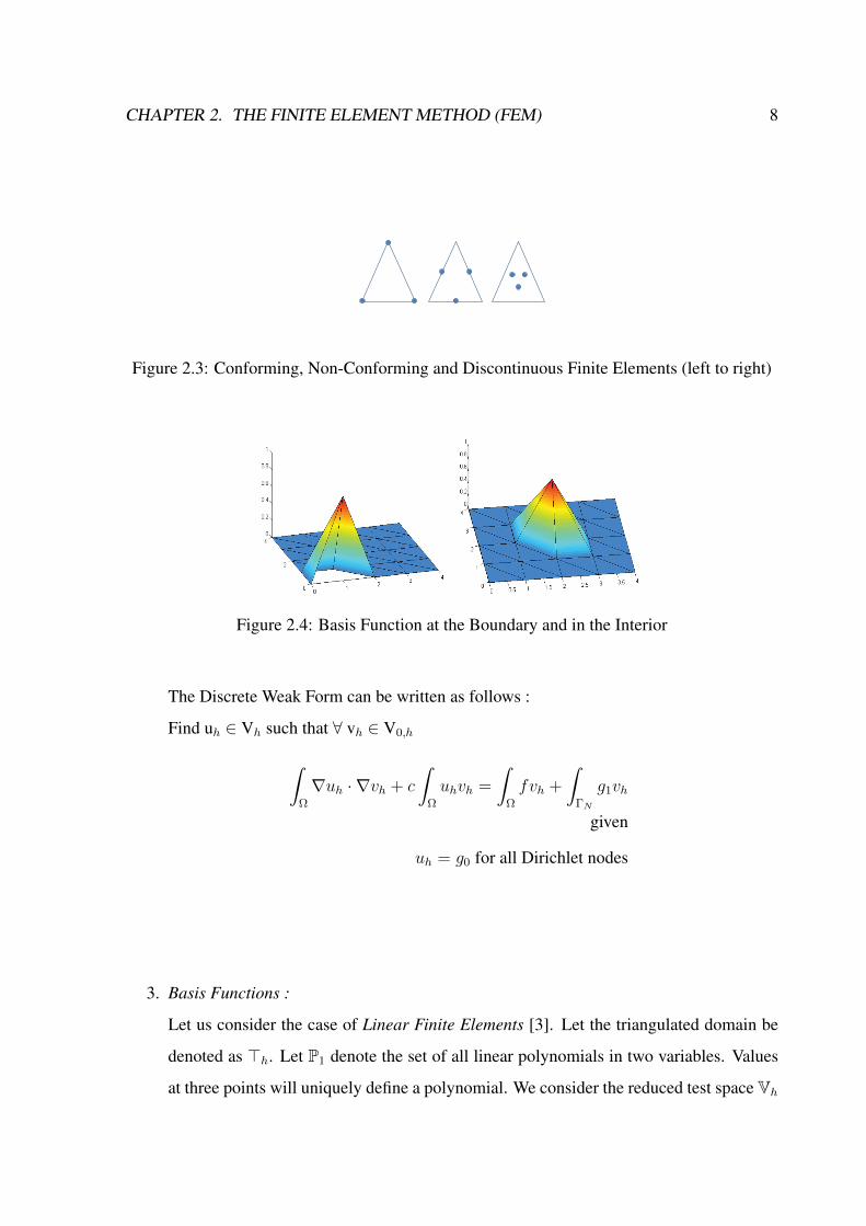
There are three types of Finite Elements (Figure 2.3):

1. Conforming Finite Elements - Degrees of freedom may lie on vertices,edges and

int the interior

2. Non-Conforming Finite Elements - Degrees of freedom lie only on the edges

3. Discontinuous Finite Elements - Degrees of freedom lie only in the interior of the

cell

Let us consider the case of P1 finite elements.

Let p ∈ P1 = a0 + a1x1 + a2x2 | a0, a1, a2 ∈ R

Vh = uh ∈ C(Ω) | uh|K ∈ P1, ∀K ∈ Th

V0,h = uh ∈ Vh | uh = 0 ∀ Dirichlet nodes

Thus Vh is the space of all piecewise linear continuous functions over the domain.


Figure 2.3: Conforming, Non-Conforming and Discontinuous Finite Elements (left to right)

Figure 2.4: Basis Function at the Boundary and in the Interior

The Discrete Weak Form can be written as follows :

Find uh ∈ Vh such that ∀ vh ∈ V0,h∫Ω

∇uh · ∇vh + c

∫Ω

uhvh =

∫Ω

fvh +

∫ΓN

g1vh

given

uh = g0 for all Dirichlet nodes

3. Basis Functions :

Let us consider the case of Linear Finite Elements [3]. Let the triangulated domain be

denoted as >h. Let P1 denote the set of all linear polynomials in two variables. Values

at three points will uniquely define a polynomial. We consider the reduced test space Vh


as the set of all continuous piecewise linear functions i.e. these functions are linear on a

triangle and continuous across the triangulation. The basis functions for this test space

is taken as :

ϕi(pj) = δij =

1 if j = i

0 if j 6= i

Note pi are the vertices of the triangle. Any function uh in test space Vh can be written

as a linear combination of the basis functions

uh(x) =N∑j=1

ujϕj(x)

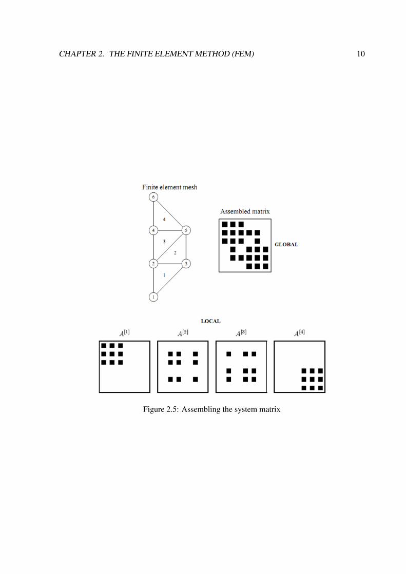
4. Assembling the system of equations :

Using the discretized equation the system matrix is assembled. The system is a sparse

system as the basis functions chosen have their support only on the cells containing the

Degree of Freedom (shown in Fig 2 and Fig 3). It is zero elsewhere. The boundary

conditions are also imposed. Every cell assembles its own local matrix which is then

assembled into the global matrix. The assembling of the local and global matrix is

shown in Figure 2.5.

5. Solving the system of equations :

The Assembled system of equations is then solved either using an exact method or an

iterative approach.


Figure 2.5: Assembling the system matrix

Chapter 3

Domain Decomposition and Parallel

Implementation

3.1 ParMooN

ParMooN [1] is the parallel version of the finite element package MooNMD (Mathematics

and object oriented Numerics in MagDeburg) which is written in object-oriented C++ for

solving two-dimensional and three-dimensional scalar convection diffusion and Navier-Stokes

equations that arise in Computational Fluid Dynamics (CFD). [2]

3.2 Domain Decomposition

In order to parallelize the Finite Element scheme, we must first triangulate the domain into the

required finite element cells. The domain is stored in ParMooN using the class Domain. This

class contains all the required information regarding the geometry of the domain. Information

such as dimensions of the domain, shape of the domain, etc. are provided to the class from the

.PRM and .GEO files which define the topology and dimensions of the domain. The domain

is then triangulated into the required number of cells.

Note that the entire domain is initially contained in all the processors. ParMooN uses an exter-

nal Mesh Partioning software called METIS. The triangulated domain is given as an input to

11

CHAPTER 3. DOMAIN DECOMPOSITION AND PARALLEL IMPLEMENTATION 12

Figure 3.1: Support of basis functions associated with a Degree of Freedom on the vertex, edgeand interior of the element

METIS, which basically partitions the finite element mesh and assigns a processor number to

every cell in the domain. Using the output from METIS every processor determines the cells

assigned to it. These cells are known as Own Cells.

Own DOFs are defined as the DOFs contained in the cells assigned to the respective processor,

i.e . the Own Cells. Every processor calculates the solution of its Own Degrees of Freedom

(Own DOFs) accurately.

As shown in Figure 3.1 a DOF has its support in all finite elements that contain the DOF.

Therefore, for a processor to calculate the solution at all its Own DOFs accurately it must con-

tain all the cells containing the Own DOFs. Hence, in addition to its Own Cells every processor

must contain the Halo cells too. Halo Cells are cells which share an edge or vertex with any

of the Own Cells. Hence for every processor the total number of cells it contains is given by :

Total Cells = Own Cells + Halo Cells

These cells are stored as a collection in the domain and the rest are deleted. In this way every

processor now contains only its Own Cells and Halo Cells. The Finite Element (FE) space is

constructed over all these cells. Depending on the type of Finite Element to be constructed the

number of DOFs per cell and their positions vary. The DOFs may lie on the vertex, edge or in

the interior of the cell.


0

00

0

00

0 00

0

0

0

0

0 0

00

0

0

00

0

00

0 0

0

0 0

0

0 0

00

0 0

0

00

0 0

0 0

00

0

00

0

0 0

00

0

00

0

00

0 0

0

0 0

03

3

3

3

13

33

3

33

1 1

1 11

1 1 1

1 1

1 11

1 1

1

1 1

1

1 11

1 1 11

1 1

11

1 1

1

1 1

1

1 1

11

1

11

11

1

1

1

1 1 1

11

1

1

1

1

11

1

11

1 1

1

1 1

1

1 1

11

1

3

3 0

0 0

0

00

0 0

0 00

2

2

2

2

22

2

22

22

3

2

2 2

2

2 2

22 2

2

2

2

22

2

2

2

2 2

2

2

2 2

2

2 2

22

2

22

2

22

2 2

222 2

22

22

2 2

2

2

2

22

2 2

2

2 2

2

2 2

22

2

22

2 1

1

1

1

1 1

11

1

1

13 33 3

13

3

3

33

3 3

33

3

33

3

33

3 3

3

3 3

3 3

3

3

3

3

3

3

3 3

3

3

33

3

3 3

3

3 3

33

3

33

3

33

3 3

3 3

33

3

33

3

3 33 3

3

3

3 3

33

0

0

0

0

1

0

0

00

0

222 2

1

22

2

2

2

2

Figure 3.2: Mesh partition using METIS : The green colored cells denote the Halo Cells andthe red colored cells denote the Dependent Cells

3.3 FE Communicator

Master and Slave DOFs

Every DOF that lies on the edge or vertex of a cell is shared by more than one cell. The Cells

sharing the DOF may belong to different processors. Hence it is important to determine which

processor should take the responsibility of calculating the solution at the DOF. The processor

which takes the responsibility of calculating the solution at the DOF is known as the Master

of the DOF and rest of the processors sharing the DOF are called Slaves.

The processor with the least rank is assigned as the Master of the DOF. After every step of an

iterative method it is the duty of the Master processor to send the value of the DOF to all the

Slave processors. In this way before the next iteration all the processors will have the updated

value of the DOF.

Every processor calls the FE Communicator. It is the job of the FE Communicator to determine

the DOFs for which the calling processor is assigned as the Master (Master DOFs) and the

DOFs for which the processor is assigned as the Slave (Slave DOFs). The DOFs which are

shared by cells, all belonging to same processor are Local DOFs of the respective processors.


The total number of DOFs in a processor is given by :

Total DOFs = Master DOFs + Slave DOFs + Local DOFs

Mapping of DOFs across processors

In order to solve the system of equations generated from the FE Space the processor must

receive all the updated values of its Slave DOFs from their respective Master processors. In

the same way the processor must send all updated values of its Master DOFs to their respective

Slave processors. These communications are done using the MPI Alltoall and MPI Alltoallv

functions [4]. The main task of the FE Communicator is to map the incoming information to

the correct DOFs. To handle this task we will be using three terms:

i Global Cell Number - The same cell will have the same Global Cell Number across all

processors

ii Localp Index - Index of a DOF in a processor. Different across all processors

iii Localc Index - Index of a DOF in a cell. Different across cells containing the DOF

Before partitioning the domain every cell in the domain is assigned a number. This number

is known as the Global Cell Number. After partitioning too, every cell retains this number.

On creation of the FE Space over all the cells in the processor (Own Cells + Halo Cells)

each DOF is associated with two indices. One denotes the index of the DOF in the processor

(Localp Index) and the other denotes the index of the DOF in the cell (Localc Index) to which

it belongs. The Localc Index will be different for every cell which contains the DOF. However

the Localc Index of a DOF for a particular cell is consistent across all processors. Therefore,

a DOF can be uniquely defined by the Global Cell Number of one of the cells to which it

belongs and its corresponding Localc Index in that cell. Along with the data of the DOF to be

communicated the Global Cell Number and corresponding Localc Index of the DOF should

also be communicated.


Algorithm 1 Pseudo Parallel Code

1. Initialize Domain from .PRM and .GEO files

2. Triangulate Domain into cells.

3. Partition the Domain using METIS

4. Using o/p of METIS determine Own Cells and Halo Cells

5. Keep Own Cells + Halo Cells. Delete the rest

6. Create Finite Element Space over these cells

7. Create FE Communicator

8. Assemble matrix

9. Solve the system of equations using an iterative solver like Jacobi and Gauss-Siedel

10. while‖xnew − xold‖‖xold‖

> ε

i. Perform an iteration of the iterative solver

ii. Update values of Slave DOFs using FE Communicator

end while

3.4 Solving the System of Equations using Parallel Iterative

Solver

After mapping the received information to the respective DOFs we solve the assembled sys-

tem of equations (Ax = b) using an iterative method like the Jacobi Method and the Gauss-

Siedel Method. The matrix A and RHS b are given as input. The matrix A is of size (Total

DOFs)x(Total DOFs) and b is a vector of size Total DOFs. Before giving the inputs it is

important to make the necessary changes in the rows corresponding to the Slave DOFs. The

values of the Slave DOFs are not caluclated in the Slave processors but received from the

respective Master processor via the FE Communicator. All non-diagonal entries in the rows

corresponding to the Slave DOFs are made zero and the diagonal entry is set to 1. In vector b

the entry corresponding to the Slave DOF is set to the value received from its Master processor.


After making these necessary changes the matrix A and vector b (rhs) are given as input to the

direct solver. Note that the changes in matrix A need to be made only once as the Slave DOFs

are known to the processor. The Slave DOFs do not change after every iteration. The rhs b

however, has to be updated with the most recent value after every iteration. After every iter-

ation the updated values are communicated using the procedure Comm→Update(rhs,solution)

Algorithm 2 Finite Element(FE) Communicator

1. INPUT : MPI Communicator and Finite Element Space

2. Find Master of each DOF (least rank processor is assigned the Master)

3. Identify the Slave DOFs and calculate number of Slave DOFs

4. Store the Global Cell Number and the corresponding Localc Index of all the Slave DOFsand Master DOFs

5. Send information of the Master DOFs to the respective Slave processors

6. Receive information regarding Slave DOFs from their respective Master processors

7. Map the received information to the Slave DOFs using the Global Cell Number and thecorresponding Localc Index

8. Store this mapping for further communications


Figure 3.3: Flowchart describing Algorithm 1 for Parallel Code


Figure 3.4: Flowchart describing Algorithm 2 for FE Communicator

Chapter 4

Multigrid Solver

Multigrid (MG) methods in numerical analysis are a group of algorithms for solving differen-

tial equations using a hierarchy of discretizations. The main idea of multigrid is to accelerate

the convergence of a basic iterative method by global correction from time to time, accom-

plished by solving a coarse problem. This approach has the advantage over other methods that

it often scales linearly with the number of discrete nodes used. It can solve these problems to a

given accuracy in a number of operations that is proportional to the number of unknowns.There

are many variations of multigrid algorithms, (Geometric Multigrid and Algebraic Multigrid)

but the common features are that a hierarchy of discretizations (grids) is considered. The steps

involved are:

1. Smoothing − reducing high frequency errors, for example using a few iterations of the

GaussSeidel method.

2. Restriction − downsampling the residual error to a coarser grid.

3. Interpolation or prolongation − interpolating a correction computed on a coarser grid

into a finer grid.

The Jacobi and Gauss-Seidel iterations produce smooth errors. The error vector e has its

high frequencies nearly removed in a few iterations. But low frequencies are reduced very

slowly. Convergence requires O(N2) iterations, which can be unacceptable. The extremely

effective multigrid idea is to change to a coarser grid, on which low frequencies act like higher

19

CHAPTER 4. MULTIGRID SOLVER 20

Figure 4.1: Two Grid and Multigrid V-cycle

frequencies. On that coarser grid a big piece of the error is removable. We iterate only a few

times before changing from fine to coarse and coarse to fine. The result is that multigrid can

solve many sparse and realistic systems to high accuracy in a fixed number of iterations, not

growing with n. The basic steps involved in a Multigrid V-Cycle algorithm are:

1. Iterate on Ahu = bh to reach uh (say 3 Jacobi or Gauss-Seidel steps).

2. Restrict the residual rh = bh − Ah uh to the coarse grid by r2h = R2hh rh .

3. Solve A2h E2h = r2h (or come close to E2h by 3 iterations from E = 0).

4. Interpolate E2h back to Eh = Ih2h E2h . Add Eh to uh .

5. Iterate 3 more times on Ahu = bh starting from the improved uh + Eh .

4.1 The Restriction and Prolongation Operators

The Restriction and Prolongation operators are interpolation matrices. There are two types of

Restriction operators :

CHAPTER 4. MULTIGRID SOLVER 21

• Pointwise Restriction : In Pointwise Restriction the function values at the matching

nodes are directly copied. The quality of the restriction is not good.

• Weighted Restriction : In Weighted Restriction or full weighting a weighted average

of the function values all the surrounding nodes is used to determine the value at the

corresponding coarse node

4.2 Computational Complexity

The number of operations performed in the V-Cycle on each grid is proportional to the number

of degrees of freedom. Because the number of variables at each grid is approximately a con-

stant fraction of that of the next finer grid (one-half in 1D and one-fourth in 2D), the total

number of operations per V-Cycle is greater than the number of operations performed on just

the finest grid only by a constant factor. In 1D, this factor is bounded by (1 + 1/2 + 1/4 + ...

=) 2, and in 2D by (1 + 1/4 + 1/16 + ... =) 4/3. Let us denote the amount of computation

required for a single Jacobi relaxation on the finest grid (or a calculation of the residual, which

is approximately the same) by a work unit(WU). We perform three iterations of the Jacobi

relaxation on the fine grids. Hence, we require three WUs for relaxation on the finest grid

and one more for computing the residual. The prolongation plus the restriction operations

together require no more than one WU. We perform pre-smoothing on the fine grids before

restriction and post-smoothing after prolongation. We also require to calculate the residual

before performing Restriction. Thus, the fine-grid work is approximately eight WUs per V-

Cycle. Finally, observe that on each multigrid level in the hierarchy, the operations (relaxation,

prolongation and restriction) can be performed in parallel. Thus, the number of sequential steps

required by the V-Cycle is proportional to the number of levels, which is O(log2 N) in our case

(considering a unit square domain with Q1 finite elements. [9]

Chapter 5

Implementation of Multigrid Solver in

ParMooN

5.1 Creation of Hierarchy of Meshes in Parallel

A Multigrid V-Cycle is implemented to solve the system of equations generated by the Finite

Element Method. After performing few iterations on the fine grid, the residual equation is

solved on the coarser levels. The correction at the coarser levels is prolongated back to the

finer levels for a better initial guess. Few more iterations are performed on the finer level with

the improved initial guess.

A certain level of refinement is initially fixed for the coarsest level. The domain in every pro-

cessor is then refined till the coarsest level refinement is achieved. The mesh is then partitioned

and every processor keeps its own sub-domain along with the halo cells.

The coarsest level is then refined (along with the halo cells) step by step until the finest level

mesh is reached.

5.2 Components of a Multigrid Level

The refinement of Halo cells at every level creates few unwanted cells (cells which have no

Own cells as their neighbour). The unwanted cells created are removed by the Domain Crop

22

CHAPTER 5. IMPLEMENTATION OF MULTIGRID SOLVER IN PARMOON 23

routine (Figure 5.2). Two FE Spaces are created at every level of refinement. One FE Space

is constructed only over the Own Cells (excluding the Halo Cells) called the OwnFESpace

and the other is constructed over the entire sub-domain (including the Halo cells) called the

CompleteFESpace. A Parallel FE Communicator is built for every level to facilitate the com-

munication amongst processors.

Algorithm 3 Pseudo Parallel Multigrid Code

1. Refine the domain till the coarsest level in each processor

2. Partition mesh

3. Every processor keeps its Own Cells along with the Halo Cells

4. Loop until finest level is reached

i. Refine the domanin another level

ii. Crop the domain (Remove unwanted halo cells after refinement)

iii. Construct two FE Spaces : OwnFESpace (excluding Halo Cells) and CompleteFES-pace (including Halo Cellls)

iv. Build the Parallel FE Communicator for the CompleteFESpace

5. Call the Parallel Multigrid Solver

5.3 Mapping Strategy in Parallel

As discussed earlier in the section of FE Communicator a DOF can be uniquely identified by

providing the Global Cell Number of a cell containing the DOF and the corresponding Localc

Index of the DOF in that cell. However in the multigrid case consistency of the Global Cell

Number across the processors will be maintained only at the coarsest level. After cropping the

domain at the coarsest level, the refinement of the domain is local to every processor. Hence

in the multigrid case we assign the Global Cell Number using the relationship given below :

GCN(i) = PGCN(i−1) ×NC + CI


where

GCN(i) − Global Cell Number of a cell at level i

PGCN(i−1) − Global Cell Number of the parent of the cell at (coarser) level i-1

NC − Number of children each cell has

CI − Child index of the cell w.r.t. its parent

The above formulation guarantees a unique Global Cell Number for every cell across all

processors. Each level along with the two FE Spaces and a Parallel FE Communicator consti-

tute one Multigrid level. The system of equations at each level is solved on the Complete FE

Space whereas the Restriction and Prolongation operations are performed on the OwnFES-

pace. This completes the creation of a hierarchy of meshes with all the necessary components.

5.4 Parallel Multigrid V-Cycle

Each processor calls the Multigrid Solver after the hierarchy of meshes is created. The Solver

begins by performing few iterations on the finest mesh to smoothen out the high frequency er-

ror components. After every iteration of the pre-selected iterative solver the updated values are

communicated using the Parallel FE Communicator. This step is known as the Pre-Smoothing

step. The residual is then restricted to the coarser level. However the restriction cannot be per-

formed on the CompleteFESpace as the dimensions of the CompleteFESpace is not consistent

across the multigrid levels (because of the removal of unwanted halo cells). Hence the residual

values are first copied from the CompleteFESpace onto the OwnFESpace and then Restriction

is performed on the OwnFESpace.

At the coarser level the values are copied back from the OwnFESpace to the CompleteFESpace

and values on the Halo Cells are updated across the processors using the FE Communicator.

The residual equation is solved (with the 0 vector as an initial guess) on the coarser mesh. The

Pre-Smoothing and Restriction steps are repeated until the coarsest level is reached. The resid-

ual equation is solved exactly (or upto a predefined level of accuracy) on the coarsest mesh.

This correction is prolongated back to the finer level. Similar to Restriction, Prolongation


cannot be performed on the CompleteFESpace. Hence the values are copied from the Com-

pleteFESpace to the OwnFESpace and then prolongated back to the finer level. At the finer

level the values are copied back from the OWnFESpace to the CompleteFESpace. The values

on the Halo Cells are updated across the processors using the FE Communicator. Few more

iterations are run on the finer mesh with the new improved initial guess. This step is known

as Post-Smoothing. The Prolongation and Post-Smoothing operations are performed on each

level till the finest mesh is reached.

This completes one Multigrid V-cycle, which gives us the next fixed point in a Fixed Point

Iteration.

Algorithm 4 Parallel Multigrid Solver : (V−Cycle)

1. INPUT:

i. OwnFESpace and CompleteFESpace of each Multigrid level

ii. Parallel FE Communicator of each Multigrid level

2. Repeat till coarsest level is reached

i. Pre−Smoothing : Reduce high frequency errors by performing few iterations of Jacobior Gauss−Siedel method

ii. Update defect across processors using parallel FE Commmunicator

iii. Copy residual values from CompleteFESpace to OwnFESpace

iv. Restrict residual values from Fine level to Coarse level. Restriction is performed onOwnFESpace

3. Solve the residual equation exactly at the coarsest level either by using a Direct Solver orby using an Iterative Solver until convergence to solution is achieved

4. Repeat till finest level is reached

i. Prolongate the solution of the residual equation at the coarse level to the fine level andadd it to the previous approximate solution. Prolongation is performed on OwnFES-pace

ii. Copy residual values from OwnFESpace to CompleteFESpace

iii. Update the improved solution across processors using parallel FE Commmunicator

iv. Post−Smoothing : Reduce high frequency errors by performing few iterations of Ja-cobi or Gauss−Siedel method with the new improved initial guess


Figure 5.1: Part I: Initialization of domain in each processor

Figure 5.2: Part II: Construction of Multigrid Levels


Figure 5.3: Flowchart for Parallel Multigrid V-Cycle

Chapter 6

Results and Conclusion

Test Example :

−4uPe

+ b · ∇u+ cu = 0

Ω = (0, 1)2

u = 0 on ∂Ω\ΓN

∂u/∂n = 0 on ΓN

b = [1 1]

c = 0.5

Pe = 100

where Pe is the Peclet number

Analytical Solution : u(x, y) = sin(πx)sin(πy)

6.1 Sequential and Parallel Results

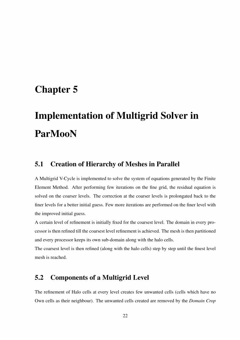
The sequential solution of the problem considered is presented in the first part of Figure 6.1.

The parallel solution obtained with four processors is presented in Figure 6.1.

28

CHAPTER 6. RESULTS AND CONCLUSION 29

Figure 6.1: Sequential Solution along with Parallel solution in all 4 processors

6.2 Parallel Multigrid experiments

Setup :

The Parallel Multigrid code was run with 2,4,8,16 and 32 processors. The grid size for the

problem was varied from 16 × 16 to 2048 × 2048. Note these are the grid sizes and not the

size of the system generated from these grids (which is much larger as mentioned in Table 6.1).

The test example was run using both conforming and non-conforming finite elements. Results

for both linear and quadratic finite elements was generated.

Findings :

The time required to solve the system was noted and compared with the sequential times to

calculate the speedup.

Speedup =Time required by sequential code

Time required by parallel code

The principal benefit obtained by increasing the number of processors is that, the system solved

by each of the processor is small. However communication overhead increases. Thus there is

a trade off between the number of processors and communication overhead for a given grid

size.


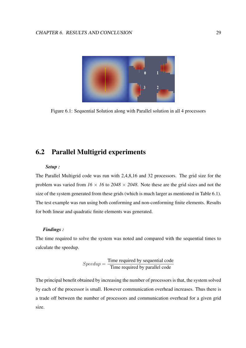
GridSize

LinConf

QuadConf

LinNon-Conf

QuadNon-Conf

16 289 1089 544 134432 1089 4225 2112 524864 4225 16641 8320 20736128 16641 66049 33024 82432256 66049 263169 131584 328704512 263169 1050625 525312 13127681024 1050625 4198401 2099200 52469762048 4198401 16785409 8392704 20962842

Table 6.1: Size of system (Number of DOFs) with varying grid size and finite element type

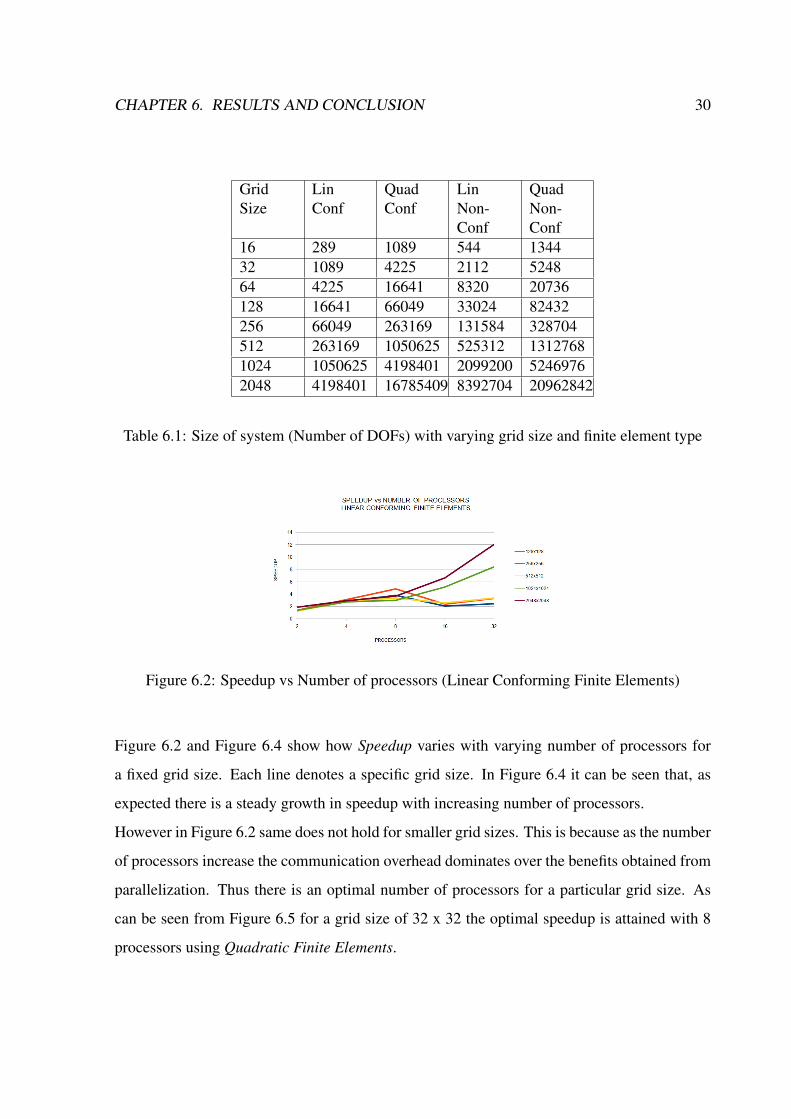
Figure 6.2: Speedup vs Number of processors (Linear Conforming Finite Elements)

Figure 6.2 and Figure 6.4 show how Speedup varies with varying number of processors for

a fixed grid size. Each line denotes a specific grid size. In Figure 6.4 it can be seen that, as

expected there is a steady growth in speedup with increasing number of processors.

However in Figure 6.2 same does not hold for smaller grid sizes. This is because as the number

of processors increase the communication overhead dominates over the benefits obtained from

parallelization. Thus there is an optimal number of processors for a particular grid size. As

can be seen from Figure 6.5 for a grid size of 32 x 32 the optimal speedup is attained with 8

processors using Quadratic Finite Elements.


Figure 6.3: Speedup vs Grid Size (Linear Conforming Finite Elements)

Figure 6.4: Speedup vs Number of processors (Quadratic Conforming Finite Elements)

Figure 6.5: Speedup vs Grid Size (Quadratic Conforming Finite Elements)


Figure 6.6: Speedup vs Number of processors (Quadratic Conforming Finite Elements)

Figure 6.7: Scalability Measure for 32 Processors


More on Speedup :

However from Figure 6.4 it can be seen that a speedup of 11 is achieved with 32 processors

for a grid size of 2048 x 2048. Ideally the speedup should have been 32. The reason for this is

mainly the Iterative Solver used in the Parallel Multigrid algorithm. We have used the Jacobi

(or weighted Jacobi for quadratic finite elements) Iterative solver. Thus after every iteration

of the Jacobi method (done independently by each processor) the updated values need to be

communicated. Thus for every iteration there is an extra communication overhead. Hence we

compared the time required per iteration as opposed to the time required for communication

in one iteration. The Scalability Measure with 32 processors is presented in Figure 6.7 for

Quadratic Finite Elements. It can be seen that the ratio keeps increasing as grid size increases

which enhances the scalability of the algorithm implemented.

Conclusion and Future Work:

An efficient data structure for implementing Multigrid in parallel has been constructed and

studied. In future, the parallel Multigrid algorithm can be implemented and studied for Dis-

continuous Finite Elements. In Discontinuous finite elements all the DOFs lie in the interior

thus reducing communication overhead considerably. However the number of DOFs increase

considerably resulting in increasing computational cost.

Bibliography

[1] V. John, G. Matthies, “MooNMD - a program package based on mapped finite element

methods”, Comput. Visual. Sci. 6, 163 - 170, 2004

[2] S. Ganesan, “Finite element methods on moving meshes for free surface and interface

flows”

[3] Mark S. Gockenbach, “Understanding And Implementing the Finite Element Method”,

SIAM, July 1, 2006

[4] Marc Snir, Steve W. Otto, David W. Walker, Jack Dongarra, Steven Huss-Lederman,

“MPI: The Complete Reference”, The MIT Press, 1996

[5] Klaus-Jurgen Bathe, “Finite Element Procedures”, Prentice Hall, June 26, 1995

[6] Yousef Saad, “Iterative Methods for Sparse Linear Systems”, SIAM, January 3, 2000

[7] W.L. Briggs, A Multigrid Tutorial, SIAM, Philadelphia, 1987

[8] P. Wesseling, An introduction to multigrid methods, John Wiley, Chichester, 1992

[9] Irad Yavneh, “ Why Multigrid Methods Are So Efficient”, Computing in Science and

Engineering,2006

[10] http://ocw.mit.edu/courses/mathematics/18-086-mathematical-methods-for-engineers-ii-

spring-2006

[11] en.wikipedia.org

34

Parallel Multigrid Solver for Large Sparse Linear Systems (08378)_Project... · Parallel Multigrid...

Documents

Transcript of Parallel Multigrid Solver for Large Sparse Linear Systems (08378)_Project... · Parallel Multigrid...