Parallel Adaptive Boundary Layer Meshing for CFD Analysis · Parallel Adaptive Boundary Layer...

Parallel Adaptive Boundary Layer Meshing forCFD Analysis

Aleksandr Ovcharenko1, Kedar Chitale2, Onkar Sahni1, Kenneth E. Jansen2,and Mark S. Shephard1

1 Scientific Computation Research Center (SCOREC), Rensselaer PolytechnicInstitute, 110 8th St, Troy, NY 12180 [email protected]

2 University of Colorado at Boulder, Boulder, CO [email protected]

Summary. This paper describes a parallel procedure for anisotropic mesh adapta-tion with boundary layers for use in scalable CFD simulations. The parallel meshadaptation algorithm operates with local mesh modification operations developedfor both unstructured and boundary layer parts of the mesh. The adaptive approachmaintains layered elements near the viscous walls and accounts for the mesh mod-ification operations that are carried out in parallel on a distributed mesh. In theprocess mesh relationships and approximations with respect to curved complex 3Dgeometries of interest are properly maintained. The parallel mesh adaptation proce-dures are applied to two problems: a heat transfer manifold and a scramjet engine.

Key words: parallel mesh adaptation, boundary layer mesh, semi-structured mesh,parallel adaptive viscous flow simulations

1 Introduction

Adaptive meshing provides a powerful tool for addressing the creation of op-timal meshes for problems such as fluid flows in which highly anisotropicsolution features can develop and only be located and resolved through adap-tivity [1–4]. It is well known that uniformly refined meshes will not yield thedesired levels of solution accuracy at an adequate computational cost and thatadaptive methods provide an effective means to create meshes that will yieldthe requested solution quality at acceptable costs [1,5,6]. One approach to thedevelopment of these adaptive meshes is to modify a given mesh to match ananisotropic mesh size field, where such a mesh size field is derived from errorcorrection indicators evaluated based on a computed solution [5–10].

Many physical problems of interest involve directional solution features,for example, boundary layers which form near the walls in viscous flows orshocks in high-speed flows. In such cases the application of anisotropic meshadaptation will yield meshes that provide the same level of accuracy with

2 Aleksandr Ovcharenko et al.

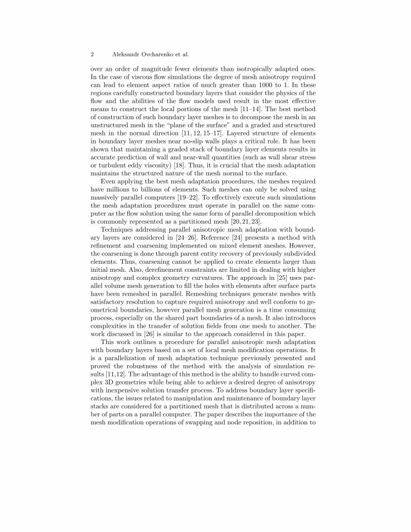
over an order of magnitude fewer elements than isotropically adapted ones.In the case of viscous flow simulations the degree of mesh anisotropy requiredcan lead to element aspect ratios of much greater than 1000 to 1. In theseregions carefully constructed boundary layers that consider the physics of theflow and the abilities of the flow models used result in the most effectivemeans to construct the local portions of the mesh [11–14]. The best methodof construction of such boundary layer meshes is to decompose the mesh in anunstructured mesh in the “plane of the surface” and a graded and structuredmesh in the normal direction [11, 12, 15–17]. Layered structure of elementsin boundary layer meshes near no-slip walls plays a critical role. It has beenshown that maintaining a graded stack of boundary layer elements results inaccurate prediction of wall and near-wall quantities (such as wall shear stressor turbulent eddy viscosity) [18]. Thus, it is crucial that the mesh adaptationmaintains the structured nature of the mesh normal to the surface.

Even applying the best mesh adaptation procedures, the meshes requiredhave millions to billions of elements. Such meshes can only be solved usingmassively parallel computers [19–22]. To effectively execute such simulationsthe mesh adaptation procedures must operate in parallel on the same com-puter as the flow solution using the same form of parallel decomposition whichis commonly represented as a partitioned mesh [20,21,23].

Techniques addressing parallel anisotropic mesh adaptation with bound-ary layers are considered in [24–26]. Reference [24] presents a method withrefinement and coarsening implemented on mixed element meshes. However,the coarsening is done through parent entity recovery of previously subdividedelements. Thus, coarsening cannot be applied to create elements larger thaninitial mesh. Also, derefinement constraints are limited in dealing with higheranisotropy and complex geometry curvatures. The approach in [25] uses par-allel volume mesh generation to fill the holes with elements after surface partshave been remeshed in parallel. Remeshing techniques generate meshes withsatisfactory resolution to capture required anisotropy and well conform to ge-ometrical boundaries, however parallel mesh generation is a time consumingprocess, especially on the shared part boundaries of a mesh. It also introducescomplexities in the transfer of solution fields from one mesh to another. Thework discussed in [26] is similar to the approach considered in this paper.

This work outlines a procedure for parallel anisotropic mesh adaptationwith boundary layers based on a set of local mesh modification operations. Itis a parallelization of mesh adaptation technique previously presented andproved the robustness of the method with the analysis of simulation re-sults [11,12]. The advantage of this method is the ability to handle curved com-plex 3D geometries while being able to achieve a desired degree of anisotropywith inexpensive solution transfer process. To address boundary layer specifi-cations, the issues related to manipulation and maintenance of boundary layerstacks are considered for a partitioned mesh that is distributed across a num-ber of parts on a parallel computer. The paper describes the importance of themesh modification operations of swapping and node reposition, in addition to

Parallel Adaptive Boundary Layer Meshing for CFD Analysis 3

refinement and coarsening, which allow matching the requested anisotropicsize field and increasing the mesh quality. Finally, the paper studies the scal-ability of parallel mesh adaptation approach on different 3D geometries.

The organization of the paper is as follows. Section 2 describes the basicanisotropic mesh adaptation concepts for the meshes with boundary layers.Section 3 discusses the parallel implementation of the mesh modification oper-ations. Section 4 shows the application of parallel anisotropic mesh adaptationprocedures to two CFD problem cases.

Nomenclature{Md}

the set of topological mesh entities of dimension d. d = 0: vertex,d = 1: edge, d = 2: face, and d = 3: region.

Mdi the ith mesh entity of dimension d.{Md

i

{MD

}}the set of mesh entities of order D adjacent to Md

i .

2 Anisotropic mesh adaptation with boundary layers

2.1 Meshes with boundary layers

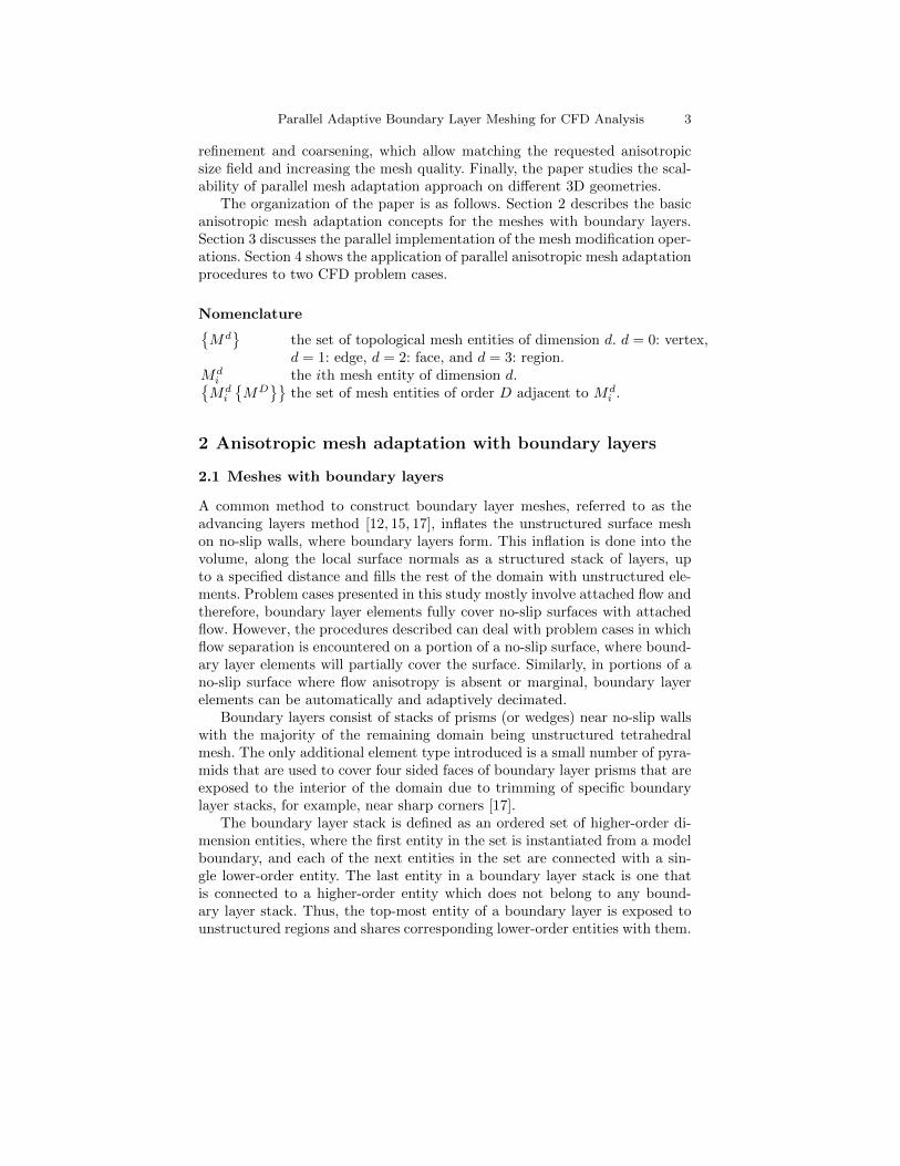
A common method to construct boundary layer meshes, referred to as theadvancing layers method [12, 15, 17], inflates the unstructured surface meshon no-slip walls, where boundary layers form. This inflation is done into thevolume, along the local surface normals as a structured stack of layers, upto a specified distance and fills the rest of the domain with unstructured ele-ments. Problem cases presented in this study mostly involve attached flow andtherefore, boundary layer elements fully cover no-slip surfaces with attachedflow. However, the procedures described can deal with problem cases in whichflow separation is encountered on a portion of a no-slip surface, where bound-ary layer elements will partially cover the surface. Similarly, in portions of ano-slip surface where flow anisotropy is absent or marginal, boundary layerelements can be automatically and adaptively decimated.

Boundary layers consist of stacks of prisms (or wedges) near no-slip wallswith the majority of the remaining domain being unstructured tetrahedralmesh. The only additional element type introduced is a small number of pyra-mids that are used to cover four sided faces of boundary layer prisms that areexposed to the interior of the domain due to trimming of specific boundarylayer stacks, for example, near sharp corners [17].

The boundary layer stack is defined as an ordered set of higher-order di-mension entities, where the first entity in the set is instantiated from a modelboundary, and each of the next entities in the set are connected with a sin-gle lower-order entity. The last entity in a boundary layer stack is one thatis connected to a higher-order entity which does not belong to any bound-ary layer stack. Thus, the top-most entity of a boundary layer is exposed tounstructured regions and shares corresponding lower-order entities with them.


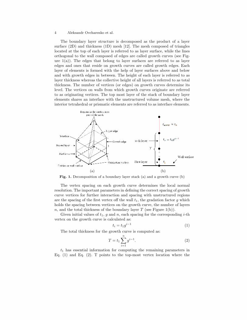
The boundary layer structure is decomposed as the product of a layersurface (2D) and thickness (1D) mesh [12]. The mesh composed of triangleslocated at the top of each layer is referred to as layer surface, while the linesorthogonal to the wall composed of edges are called growth curves (see Fig-ure 1(a)). The edges that belong to layer surfaces are referred to as layeredges and ones that reside on growth curves are called growth edges. Eachlayer of elements is formed with the help of layer surfaces above and belowand with growth edges in between. The height of each layer is referred to aslayer thickness whereas the collective height of all layers is referred to as totalthickness. The number of vertices (or edges) on growth curves determine itslevel. The vertices on walls from which growth curves originate are referredto as originating vertices. The top most layer of the stack of boundary layerelements shares an interface with the unstructured volume mesh, where theinterior tetrahedral or prismatic elements are referred to as interface elements.

(a) (b)

Fig. 1. Decomposition of a boundary layer stack (a) and a growth curve (b)

The vertex spacing on each growth curve determines the local normalresolution. The important parameters in defining the correct spacing of growthcurve vertices for further interaction and spacing with unstructured regionsare the spacing of the first vertex off the wall t1, the gradation factor g whichholds the spacing between vertices on the growth curve, the number of layersn, and the total thickness of the boundary layer T (see Figure 1(b)).

Given initial values of t1, g and n, each spacing for the corresponding i-thvertex on the growth curve is calculated as:

ti = t1gi−1 (1)

The total thickness for the growth curve is computed as:

T = t1

n∑i=1

gi−1. (2)

t1 has essential information for computing the remaining parameters inEq. (1) and Eq. (2). T points to the top-most vertex location where the


boundary layer is connected to the unstructured mesh. Note that g is a fixedconstant for a particular growth curve, however it can vary from one growthcurve to another as it is dictated by the problem boundary definition. Mean-while, spacing of the last growth edge of the growth curve tn is used to verifythe ratio between the last growth edge on a boundary layer and the normalheight in the unstructured mesh region immediately outside the boundarylayer tunstr (see Figure 1(b)). tunstr is a meaningful value to compare with tnsince it is dictated by the requested mesh metric and the difference in the twoshould provide an acceptable gradation of the mesh at that location.

2.2 Mesh metric field

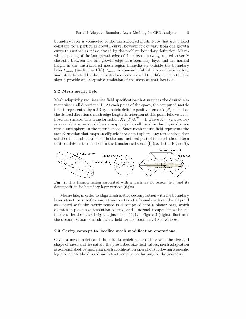
Mesh adaptivity requires size field specification that matches the desired ele-ment size in all directions [1]. At each point of the space, the computed metricfield is represented by a 3D symmetric definite positive tensor T (P ) such thatthe desired directional mesh edge length distribution at this point follows an el-lipsoidal surface. The transformation XT (P )XT = 1, where X = {x1, x2, x3}is a coordinate vector, defines a mapping of an ellipsoid in the physical spaceinto a unit sphere in the metric space. Since mesh metric field represents thetransformation that maps an ellipsoid into a unit sphere, any tetrahedron thatsatisfies the mesh metric field in the unstructured part of the mesh should be aunit equilateral tetrahedron in the transformed space [1] (see left of Figure 2).

Fig. 2. The transformation associated with a mesh metric tensor (left) and itsdecomposition for boundary layer vertices (right)

Meanwhile, in order to align mesh metric decomposition with the boundarylayer structure specification, at any vertex of a boundary layer the ellipsoidassociated with the metric tensor is decomposed into a planar part, whichdictates in-plane size resolution control, and a normal component which in-fluences the the stack height adjustment [11, 12]. Figure 2 (right) illustratesthe decomposition of mesh metric field for the boundary layer vertices.

2.3 Cavity concept to localize mesh modification operations

Given a mesh metric and the criteria which controls how well the size andshape of mesh entities satisfy the prescribed size field values, mesh adaptationis accomplished by applying mesh modification operations following a specificlogic to create the desired mesh that remains conforming to the geometry.


During the execution of a mesh modification operation it is important toclearly identify the set of mesh entities that will be affected by that modifi-cation. This set of mesh entities defines a subdomain referred to as a cavity.For the effective parallel implementation of mesh modification operations themesh modification cavity needs to be large enough that the mesh outside ofthe cavity boundary is not altered.

In a 3D domain, a single cavity C is comprised of regions adjacent to amesh entity that triggers a specific mesh modification operation and has adimension less than 3. The set of outer faces in closure of regions localized inC forms the cavity boundary which stays intact during the required alteringwithin the cavity. The application of a local mesh modification operation thenis a retriangulation of the cavity, C, into a new mesh subdomain S, whichhas the same cavity boundary as C, but contains a different set of regionscompared to original set of regions in C.

2.4 Mesh modification operations in the semi-structured part ofthe mesh

There are four major operators used for mesh modification [1,12,27], namely:split, collapse, swap and vertex repositioning. In addition, there are compoundoperators applied in the unstructured part of the mesh, which chain multiplesingle step operators in the unstructured mesh in such a manner to effectivelyyield the desired mesh configuration. The interested reader is referred to [1]for a more detailed description of mesh modifications in the unstructured partof the mesh. This paper is focuses on mesh modification procedures associatedwith the boundary layer part of the mesh.

To preserve the layered nature of boundary layer elements along the nor-mals, mesh modification for the layered part of the mesh is divided into twosteps [12]: layer surface modification and thickness adjustment. Surface meshmodification operations are propagated through the stack of boundary layerentities and affect all the layer surfaces along with the interface entities withina stack in the same way. The local mesh modification operations of edge split,collapse and swap are utilized to perform the surface mesh adaptation whilevertex repositioning is applied to adjust the layer thicknesses and move growthcurve vertices to the geometric model boundaries. The thickness adjustmentis currently in the development stage, however it is easily integrated with theset of procedures implemented to support boundary layer mesh modifications.

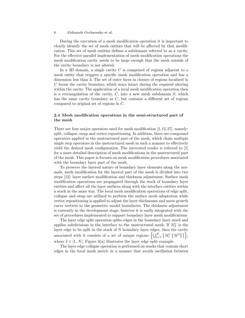
The layer edge split operation splits edges in the boundary layer stack andapplies subdivisions in the interface to the unstructured mesh. If M1

I is thelayer edge to be split in the stack of N boundary layer edges, then the cavity

associated with it consists of a set of unique regions{⋃N

i=1

{M1

i

{M3}}}

,

where I ∈ [1..N ]. Figure 3(a) illustrates the layer edge split example.The layer edge collapse operation is performed on stacks that contain short

edges in the local mesh metric in a manner that avoids oscillation between


collapse and split operations [11,12]. The edge collapse operations can only beapplied when the affected unstructured mesh entities at the top of the stackalso remain valid. If

{(M1

i ,M0i )}

are the pairs of stacks of N layer edges to becollapsed and their correspondent vertices being deleted, the cavity associated

with the collapse operator is{⋃N

i=1

{M0

i

{M3}}}

with a deletion of a set

of regions{⋃N

i=1

{M1

i

{M3}}}

. Figure 3(b) shows two boundary layers and

interface elements before and after the layer edge collapse operation.

(a) (b)

Fig. 3. Example of boundary layer split (a) and collapse (b) operations

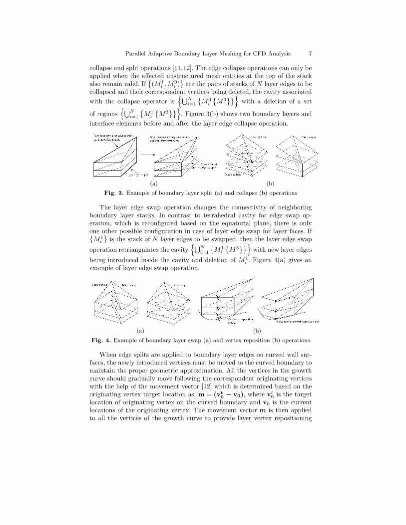
The layer edge swap operation changes the connectivity of neighboringboundary layer stacks. In contrast to tetrahedral cavity for edge swap op-eration, which is reconfigured based on the equatorial plane, there is onlyone other possible configuration in case of layer edge swap for layer faces. If{M1

i

}is the stack of N layer edges to be swapped, then the layer edge swap

operation retriangulates the cavity{⋃N

i=1

{M1

i

{M3}}}

with new layer edges

being introduced inside the cavity and deletion of M1i . Figure 4(a) gives an

example of layer edge swap operation.

(a) (b)

Fig. 4. Example of boundary layer swap (a) and vertex reposition (b) operations

When edge splits are applied to boundary layer edges on curved wall sur-faces, the newly introduced vertices must be moved to the curved boundary tomaintain the proper geometric approximation. All the vertices in the growthcurve should gradually move following the correspondent originating verticeswith the help of the movement vector [12] which is determined based on theoriginating vertex target location as: m = (vt

0 − v0), where vt0 is the target

location of originating vertex on the curved boundary and v0 is the currentlocations of the originating vertex. The movement vector m is then appliedto all the vertices of the growth curve to provide layer vertex repositioning


operation. The procedure first evaluates target locations for vertices on all thegrowth curves, with each vertex’s target location calculated as: vt

i = vi + m,where vi is the current i-th vertex location on a growth curve correspondingto its originating vertex location v0. It then moves vertices to their computedtarget locations as depicted in Figure 4(b). Similar to unstructured vertexprojection to the curved boundary, layer vertex movement through simplerepositioning is not always possible as it may introduce inverted elements,in which case local mesh modification operations are applied to the interiorvolume mesh to make the way for repositioning to be successful. After therepositioning is completed for the top most vertices, the rest of the growthcurve vertices are moved to their target locations vt

i resulting in originatingvertex being placed on its target location on the curve boundary.

2.5 Procedure of anisotropic mesh adaptation with boundarylayers

The mesh adaptation is executed in three stages: mesh coarsening, iterativemesh refinement, and shape correction [10, 12]. The first two stages are con-trolled by mesh edge length analysis in the transformed space, whereas thethird stage is dictated by both element quality and mesh edge length control.

The coarsening stage eliminates the majority of edges which are shorterthan requested by the local mesh size field. An advantage to applying thecoarsening first is that it makes the traversals required during mesh adaptationfaster and limits the peak memory usage.

The second stage refines mesh regions based on splitting mesh edges ifthey are longer when measured in the transformed space. It also places newlycreated boundary vertices on the model boundary and coarsens any new shortmesh edges introduced.

Shape correction routines improve the shape of poorly shaped entities inthe transformed space. Those entities are modified using swap / collapse /vertex reposition and compound operators [10] to obtain the best possibleelement quality while preserving the correct edge length in the metric space.

Since each pyramid is easily decomposed into two tetrahedra, the meanratio [28] is used to measure the quality of unstructured regions in the trans-formed space, namely:

η′ = 15552V ′

2(∑6i=1 l

′2i

)3 , (3)

with V ′ and l′2i being the volume and edge length square of a tetrahedron in

the transformed space. For the boundary layer part of the mesh, layer facequality control is performed, where each layer face is measured as follows:

S′ = 48A′

2(∑3i=1 l

′2i

)2 , (4)

where A′ is the layer edge face area in the transformed space.


3 Parallel implementation

3.1 Distributed mesh representation

The execution of parallel mesh adaptation is based on the fact that a singlemesh is distributed [29–31] to a number of parts that consist of a set of meshentities assigned to the corresponding processor. Each part is treated as aserial mesh with the addition of mesh part boundaries to describe groups ofmesh entities that are on inter-part boundaries.

The implementation of parallel boundary layer mesh adaptation is aidedby requiring all mesh entities in a stack to be on the same part. This process issupported by employing the entity set concept [32] in which the mesh regionsin a stack are put in a single set that must be properly maintained duringmesh modification and migration [33]. To provide proper partitioning the setis represented as one weighted node during graph partitioning.

The direct consideration of cavities on the part boundary for such meshmodification operations as collapse and swap is a complex and expensive pro-cedure since it leads to a number of communication steps to properly updatethe parts with the mesh modification decisions carried out. Thus, regions fromsuch cavities are localized on one processor. To support cavity localization, amesh migration is used, where all regions and stacks of regions involved in themesh modification operation are migrated onto a single part [20,29].

The Flexible Distributed Mesh Data Base [29] is used to support theneeded mesh-based parallel operations on distributed meshes including partboundary management and mesh migration. The Zoltan library [34] is usedfor dynamic load balancing. The Inter-Processor Communication Manager isused [35] for efficient parallel communications between processors.

3.2 Refinement and vertex reposition to geometrical boundaries

Mesh edges and their adjacent mesh faces on part boundaries are subdividedthe same way as it is done in serial since replicated faces across part boundarieshave their bounding edges and vertices in the same order such that the entitiesproperly match [20, 36]. Note that triangular faces can be split using anycombination of edges tagged for refinement, whereas quadrilateral faces aspart of the boundary layer stack, are limited to be bisected in a layer surfacedirection only, without subdivision of growth curve edges.

Each subdivision of an entity on the part boundary is matched with thesame subdivision on the part the entity is shared with. The inter-part links be-tween newly created mesh entities are appropriately updated across the partboundary [36]. The algorithm involves the same logic of updating inter-partlinks for both boundary layer and unstructured parts of the mesh. The onlydifference for the boundary layer procedure is that once the stack of quadri-lateral faces exposed to the part boundary is split, each has to be completelyupdated with the pair or copy on another part.


After refinement is completed, each part holds a list of mesh vertices that-need to be projected onto the solid model boundaries [20]. For the boundarylayer part of the mesh, the newly created originating vertices are projectedonto the solid model surfaces with the help of the movement vector as de-scribed in Section 2.4. In parallel, the migration might be involved, to com-plete the local mesh modification procedures in order to move the vertices inthe corresponding stacks for the correct vertex adjustment.

3.3 Coarsening and surface optimization

Layer edge collapse operation is performed on the on-part localized cavity. Thevicinity of boundary layer stacks sharing vertices of the same growth curvefrom a specific originating vertex M0

d to its associated top most growth curvevertex M0

dtopand their adjacent layer edges shorter than the desired size in a

metric space are checked for the layer edge collapse. If neither of the stack oflayer edges adjacent to M0

d ..M0dtop

can be collapsed locally, the boundary layercoarsening procedure migrates all the boundary layers and interface regionsadjacent to growth curve vertices from M0

d to M0dtop

to one part and checksfor the possibility of layer edge collapse operation with the full local cavity.

Figure 5 shows the example of layer edge collapse operation requestingmesh migration. It can be seen from the picture that the top-most vertexM0

dtopfor surrounding boundary layers is located on the part boundary and

layer edge collapse for its adjacent edges cannot be evaluated. Thus, M0dtop

requests all the adjacent boundary layer stacks and interface regions to bemigrated onto the part P2 such that the layer edge collapse operation can beexecuted. Different line colors indicate shared entities between specific parts.

At the end of mesh adaptation, the boundary layer surface optimizationstep is provided [12]. The logic for the optimization operation on the partboundary is similar to the layer edge collapse one as it acquires the cavityassociated with the operation locally on the part. The difference for the surfaceoptimization compared to coarsening is that the procedure calculates shapes oflayer faces (see Eq. (4)) and determines which operation should be applied tothe adjacent layer edges in order to improve the boundary layer faces quality.

4 Application results

The capabilities of the parallel anisotropic mesh adaptation with boundarylayers developed in this work are demonstrated with two CFD applications.In the first case, simulations were performed on a heat transfer manifold andmesh convergence was studied in terms of pressure drops between inlet andmultiple outlets. The other case involves a scramjet simulation of the NASACIAM [37] scramjet geometry. In the heat transfer manifold problem domainthe CFD analysis is performed by PHASTA [38]. The scramjet geometry wassimulated with FUN3D [39] solver.


Fig. 5. Example of parallel layer edge collapse operation involving mesh migration

The studies have been executed on Hopper Cray XE6 [40] at NationalEnergy Research Scientific Computing Center. It is configured with 2 twelve-core AMD 2.1 GHz processors per node, with separate L3 caches and memorycontrollers, 32 GB or 64 GB DDR3 SDRAM per node. Hopper has Geminiinterconnect with 3D torus topology. The 3D torus topology provides powerfulbisection and global bandwidth characteristics as well as support for dynamicrouting of messages.

4.1 Parallel anisotropic boundary layer adaptivity on a heattransfer manifold case

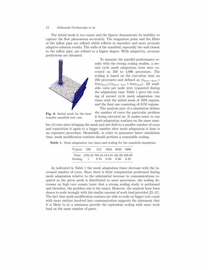
The heat transfer manifold consists of a large diameter cylindrical pipe for theinflow, a plate and twenty small outflow pipes (see Figure 6). Flow compu-tations are done using steady, incompressible RANS equations along withSpalart-Allmaras turbulence model. No-slip boundary conditions are pre-scribed on viscous surfaces and a natural pressure is assumed at outflows.Hessian matrix field based on computed solution [11] is used to form themesh metric size field in order to drive mesh adaptation procedures.

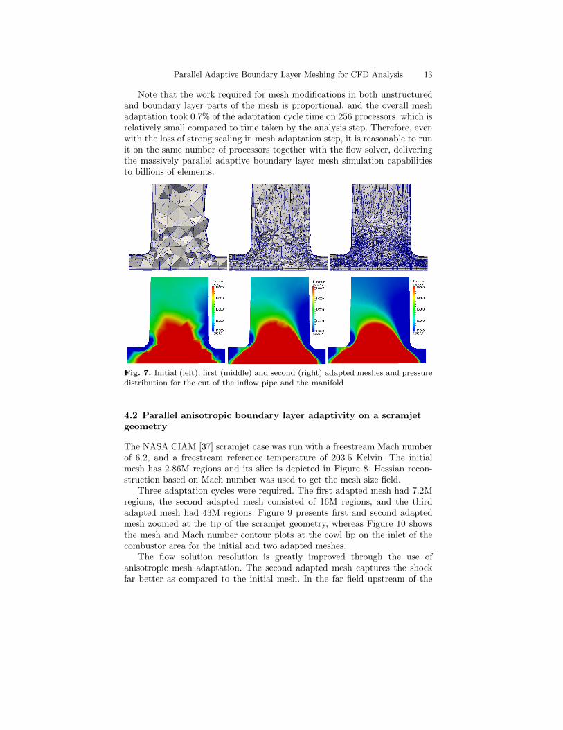
The adaptive simulation consists of a flow solve and adaptation, and iscarried out twice with the flow solve started from previous solution. Eachcycle was divided into 1000 time steps with a constant time step size of 0.1s.The initial mesh consists of 3M regions, the first adapted boundary layermesh has 16M regions, and the second adapted mesh results in 81M regions.The initial, first and second adapted inflow pipe mesh cuts with the pressuredistribution are shown on Figure 7.


The initial mesh is too coarse and the figures demonstrate its inability tocapture the flow phenomena accurately. The stagnation point and the filletsof the inflow pipe are refined which reflects in smoother and more accurateadaptive solution results. The walls of the manifold, especially the wall closestto the inflow pipe, are refined to a higher degree. With adaptivity, accuratepredictions are obtained.

Fig. 6. Initial mesh for the heattransfer manifold test case

To measure the parallel performance re-sults with the strong scaling studies, a sec-ond cycle mesh adaptation tests were ex-ecuted on 256 to 4,096 processors. Thescaling is based on the execution time on256 processors and defined as (nproc−base ∗timebase)/(nproc−test ∗ timetest). All avail-able cores per node were requested duringthe adaptation runs. Table 1 gives the scal-ing of second cycle mesh adaptation runtimes with the initial mesh of 16M regions,and the final one consisting of 81M regions.

The analysis part of a simulation definesthe number of cores the particular problemis being executed on. It makes sense to runmesh adaptation routines on the same num-

ber of cores since bringing the mesh and size field to a smaller number of coresand repartition it again to a bigger number after mesh adaptation is done isan expensive procedure. Meanwhile, in order to guarantee faster simulationtime, mesh modification routines should perform a reasonable scaling.

Table 1. Mesh adaptation run times and scaling for the manifold simulation

N/proc 256 512 1024 2048 4096

Time 1194.34 785.44 514.45 421.09 339.38Scaling 1 0.76 0.58 0.36 0.22

As indicated in Table 1 the mesh adaptation times decrease with the in-creased number of cores. Since there is little computation performed duringmesh adaptation relative to the substantial increase in communications re-quired as the given mesh is distributed to more processors, the scaling de-creases on high core counts (note that a strong scaling study is performedand therefore, the problem size is the same). However, the analysis have beenshown to scale strongly with the similar amount of work load provided [21,41].The fact that mesh modification routines are able to scale on bigger core countwith more entities involved into communication supports the statement thatit is likely to at a minimum provide the equivalent scaling with more workload on the same number of parts.


Note that the work required for mesh modifications in both unstructuredand boundary layer parts of the mesh is proportional, and the overall meshadaptation took 0.7% of the adaptation cycle time on 256 processors, which isrelatively small compared to time taken by the analysis step. Therefore, evenwith the loss of strong scaling in mesh adaptation step, it is reasonable to runit on the same number of processors together with the flow solver, deliveringthe massively parallel adaptive boundary layer mesh simulation capabilitiesto billions of elements.

Fig. 7. Initial (left), first (middle) and second (right) adapted meshes and pressuredistribution for the cut of the inflow pipe and the manifold

4.2 Parallel anisotropic boundary layer adaptivity on a scramjetgeometry

The NASA CIAM [37] scramjet case was run with a freestream Mach numberof 6.2, and a freestream reference temperature of 203.5 Kelvin. The initialmesh has 2.86M regions and its slice is depicted in Figure 8. Hessian recon-struction based on Mach number was used to get the mesh size field.

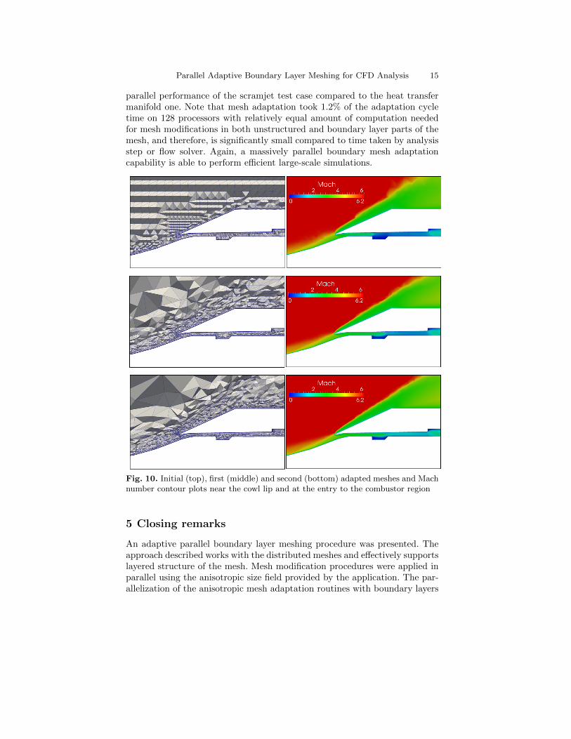
Three adaptation cycles were required. The first adapted mesh had 7.2Mregions, the second adapted mesh consisted of 16M regions, and the thirdadapted mesh had 43M regions. Figure 9 presents first and second adaptedmesh zoomed at the tip of the scramjet geometry, whereas Figure 10 showsthe mesh and Mach number contour plots at the cowl lip on the inlet of thecombustor area for the initial and two adapted meshes.

The flow solution resolution is greatly improved through the use ofanisotropic mesh adaptation. The second adapted mesh captures the shockfar better as compared to the initial mesh. In the far field upstream of the


shock, where flow is uniform and parallel, the mesh was appropriately coars-ened. Expected mesh refinement was obtained at the tips, at the cowl lip,within the combustor area, at the sharp edges of the combustor area liner,and behind the engine. Mesh anisotropy followed the shock emanating fromthe nose cone tip, with coarsening in the direction tangential to the shock.

Fig. 8. Slice of the whole (left) initial mesh and the zoom to its tip (right) for thescramjet test case

Fig. 9. Scramjet tip during the first (left) and second (right) adaptation cycles

Table 2 provides timings and strong scaling values for the mesh adaptationruns in the third adaptive cycle with input mesh of 16M regions, and the finalone consisting of 43M regions. The strong scaling studies were performed on128 to 4,096 processors. The scaling is based on the execution time on 128processors and is calculated the same way it is defined in the heat transfermanifold test case.

Table 2. Mesh adaptation run times and scaling for the scramjet test case

N/proc 128 256 512 1024 2048 4096

Time 957.80 532.29 339.39 202.17 136.83 90.85Scaling 1 0.9 0.7 0.59 0.44 0.33

Table 2 supports the observation that the mesh adaptation is able to de-crease run times with the growing number of cores. Although the simulationstudy experiences the fixed size problem phenomena on a bigger processorcount observed in the previous test case, the scalability factors show better


parallel performance of the scramjet test case compared to the heat transfermanifold one. Note that mesh adaptation took 1.2% of the adaptation cycletime on 128 processors with relatively equal amount of computation neededfor mesh modifications in both unstructured and boundary layer parts of themesh, and therefore, is significantly small compared to time taken by analysisstep or flow solver. Again, a massively parallel boundary mesh adaptationcapability is able to perform efficient large-scale simulations.

Fig. 10. Initial (top), first (middle) and second (bottom) adapted meshes and Machnumber contour plots near the cowl lip and at the entry to the combustor region

5 Closing remarks

An adaptive parallel boundary layer meshing procedure was presented. Theapproach described works with the distributed meshes and effectively supportslayered structure of the mesh. Mesh modification procedures were applied inparallel using the anisotropic size field provided by the application. The par-allelization of the anisotropic mesh adaptation routines with boundary layers


based on local mesh modifications allows the procedure to be applied to largeand complex 3D problem cases which are usually attacked with remeshingmethods. At the same time, the approach provides the ability to perform avery inexpensive solution transfer process which also allows solution not todeteriorate over the mesh adaptation cycles.

It has been demonstrated that boundary layer mesh adaptation resultedin an increase of the accuracy of key quantities of interest and helped resolvecritical areas of the flow to supply the analysis with better solution. Duringthe adaptation process, the approach was able to preserve layered elementsnear the walls and effectively account for the mesh modification operationscarried out in the distributed environment for both boundary layer and un-structured parts of the mesh, at the same time being capable of handlingcurved geometries of interest with the required mesh resolution and elementquality control.

The method described scales while utilizing different mesh modificationoperation types and not only simple refinement. The parallel performance re-sults carried out on problem domains indicate that mesh adaptation is capableof decreasing the simulation run times with higher number of cores.

6 Acknowledgements

This work was supported by the National Science Foundation under Grant No.0749152, by the U.S. Department of Energy under DOE Grant No. DE-FC02-06ER25769, and by the NASA STTR Part II Grant No. BEE103/NNX11CC69C.Computing support is provided by National Energy Research Scientific Com-puting Center for granting access to the Cray XE6 supercomputers. The au-thors would like to acknowledge F. Nihan Cayan and Oren Breslouer for theefforts in helping with the scramjet test case.

References

1. X. Li, M.S. Shephard, and M.W. Beall. 3D anisotropic mesh adaptation bymesh modifications. Comput. Method. Appl. M., 194(48-49):4915–4950, 2005.

2. G. Compere, J.-F. Remacle1, J. Jansson, and J. Hoffman. A mesh adaptationframework for dealing with large deforming meshes. Int. J. Numer. Meth. Eng.,82(7):843–867, 2010.

3. K.-J. Bathe and H. Zhang. A mesh adaptivity procedure for CFD and fluid-structure interactions. Computers and Structures, 87(11-12):604–617, 2009.

4. M. D. Piggott, G. J. Gorman, C. C. Pain, P. A. Allison, A. S. Candy, B. T.Martin, and M. R. Wells. A new computational framework for multi-scale oceanmodelling based on adapting unstructured meshes. Int. J. Numer. Meth. Fl.,56(8):1003–1015, 2008.

5. P.J. Frey and F. Alauzet. Anisotropic mesh adaptation for CFD computations.Comput. Method. Appl. M., 194(48-49):5068–5082, 2005.


6. C.L. Botasso. Anisotropic mesh adaption by metric-driven optimization. Int.J. Numer. Meth. Eng., 60(3):597–639, 2004.

7. X. Li, M.S. Shephard, and M.W. Beall. Accounting for curved domains in meshadaptation. Int. J. Numer. Meth. Eng., 58(2):247–276, 2003.

8. C.C. Pain, A.P. Umpleby, C.R.E. de Oliveira, and A.J.H. Goddard. Tetrahedralmesh optimization and adaptivity for steady-state and transient finite elementcalculations. Comput. Method. Appl. M., 190(29-30):3771–3796, 2001.

9. J.F. Remacle, X. Li, M.S. Shephard, and J.E. Flaherty. Anisotropic adaptivesimulation of transient flows using discontinuous Galerkin methods. Int. J.Numer. Meth. Eng., 62(7):899–923, 2005.

10. X. Li. Mesh Modification Procedures for General 3D Non-Manifold Domains.PhD thesis, Rensselaer Polytechnic Institute, 2003.

11. O. Sahni, J. Muller, K.E. Jansen, M.S. Shephard, and C.A. Taylor. Effi-cient anisotropic adaptive discretization of the cardiovascular system. Comput.Method. Appl. M., 195(41-43):5634–5655, 2006.

12. O. Sahni, K.E. Jansen, M.S. Shephard, C.A. Taylor, and M.W. Beall. Adaptiveboundary layer meshing for viscous flow simulations. Eng. Comput., 24(3):267–285, 2008.

13. Y. Kallinderis and C. Kavouklis. A dynamic adaptation scheme for general 3-Dhybrid meshes. Comput. Method. Appl. M., 194(48-49):5019–5050, 2005.

14. A. Khawaja, T. Minyard, and Y. Kallinderis. Adaptive hybrid grid methods.Comput. Method. Appl. M., 189(4):1231–1245, 2005.

15. C.L. Botasso and D. Detomi. A procedure for tetrahedral boundary layer meshgeneration. Eng. Comput., 18(1):66–79, 2002.

16. A. Loseille and R. Lohner. Boundary layer mesh generation and adaptivity, 2011.49th AIAA Aerospace Sciences Meeting including the New Horizons Forum andAerospace Exposition.

17. R.V. Garimella and M.S. Shephard. Boundary layer mesh generation for viscousflow simulations. Int. J. Numer. Meth. Eng., 49:193–218, 2000.

18. O. Sahni, K.E. Jansen, X.J. Luo, and M.S. Shephard. Curved boundary layermeshing for adaptive viscous flow simulations. Finite Elem. Anal. Des., 46(1-2):132–139, 2010.

19. M.S. Shephard, J.E. Flaherty, C.L. Bottasso, H.L. de Cougny, C. Ozturan,and M.L. Simone. Parallel automated adaptive analysis. Parallel Computing,23(9):1327–1347, 1997.

20. F. Alauzet, X. Li, E.S. Seol, and M.S. Shephard. Parallel anisotropic 3D meshadaptation by mesh modification. Eng. Comput., 21(3):247–258, 2006.

21. M. Zhou, O. Sahni, H.J. Kim, C.A. Figueroa, C.A. Taylor, M.S. Shephard, andK.E. Jansen. Cardiovascular flow simulation at extreme scale. ComputationalMechanics, 46(1):71–82, 2010.

22. M.S. Shephard, C. Smith, and J.E. Kolb. Bringing hpc to engineering innova-tion. Computers in Science and Engineering, 2013. Accepted for publication.http://www.scorec.rpi.edu/REPORTS/2012-1.pdf.

23. S. Chandra, X. Li, T. Saif, and M. Parashar. Enabling scalable parallel imple-mentations of structured adaptive mesh refinement applications. The Journalof Supercomputing, 39(2):177–203, 2007.

24. C. Kavouklis and Y. Kallinderis. Parallel adaptation of general three-dimensional hybrid meshes. J. Comput. Phys., 229(9):3454–3473, 2010.


25. O. Hassan, K. Sorensen, K. Morgan, and N.P. Weatherill. A method for timeaccurate turbulent compressible fluid flow simulation with moving boundarycomponents employing local remeshing. Int. J. Numer. Meth. Fl., 53(8):1243–1266, 2007.

26. S. Tendulkar, M. Beall, M.S. Shephard, and K.E. Jansen. Parallel mesh gen-eration and adaptation for CAD geometries. In Proc. of the NAFEMS WorldCongress, 2011. https://www.scorec.rpi.edu/REPORTS/2011-2.pdf.

27. C.C. Pain, A.P. Umpleby, C.R.E. de Oliveira, and A.J.H. Goddard. Tetrahedralmesh optimization and adaptivity for steady-state and transient finite elementcalculations. Int. J. Numer. Meth. Eng., 190(29-30):3771–3796, 2001.

28. A. Liu and B. Joe. On the shape of tetrahedra from bisection. Mathematics ofComputation, 63(207):141–154, 1994.

29. E.S. Seol and M.S. Shephard. Efficient distributed mesh data structure forparallel automated adaptive analysis. Eng. Comput., 22(3-4):197–213, 2006.

30. C. Ollivier-Gooch, L.F. Diachin, M.S. Shephard, T. Tautges, J. Kraftcheck,V. Leung, X. Luo, and M. Miller. An interoperable, data-structure-neutral com-ponent for mesh query and manipulation. ACM Transactions on MathematicalSoftware, 37:1–28, 2010.

31. M. Zhou, O. Sahni, K.D. Devine, M.S. Shephard, and K.E. Jansen. Controllingunstructured mesh partitions for massively parallel simulations. SIAM Journalon Scientific Computing, 32(6):3201 – 3227, 2010.

32. K.K. Chand, L.F. Diachin, X. Li, C. Ollivier-Gooch, E.S. Seol, M.S. Shephard,T. Tautges, and H. Trease. Toward interoperable mesh, geometry and fieldcomponents for pde simulation development. Eng. Comput., 24(2):165–182,2008.

33. T. Xie, S. Seol, and M.S. Shephard. Generic components for petascale auto-mated adaptive simulations. Eng. Comput., 2012. Accepted for publication.http://www.scorec.rpi.edu/FMDB/doc/xie_seol_shephard_EngComp.pdf.

34. E. Boman, K. Devine, L.A. Fisk, R. Heaphy, B. Hendrickson, V. Leung,C. Vaughan, U. Catalyurek, D. Bozdag, and W. Mitchell. Zoltan home page,2012. http://www.cs.sandia.gov/Zoltan.

35. A. Ovcharenko, D. Ibanez, F. Delalondre, O. Sahni, K.E. Jansen, C.D.Carothers, and M.S. Shephard. Neighborhood communication paradigm to in-crease scalability in large-scale dynamic scientific applications. Parallel Com-puting, 38(3):140–156, 2012.

36. H.L. de Cougny and M.S. Shephard. Parallel refinement and coarsening oftetrahedral meshes. Comput. Method. Appl. M., 46:1101–1125, 1999.

37. NASA. Ciam axisymmetric scramjet, 2012. http://hapb-www.larc.nasa.gov/Public/Engines/Ciam/Ciam.html.

38. C.H. Whiting and K.E. Jansen. A stabilized finite element method for the in-compressible Navier–Stokes equations using a hierarchical basis. Int. J. Numer.Meth. Fl., 35(1):93–116, 2001.

39. NASA. FUN3D online manual, 2012. http://fun3d.larc.nasa.gov/.40. Cray XE6, 2012. http://www.cray.com/Products/XE/CrayXE6System.aspx.41. O. Sahni, M. Zhou, M.S. Shephard, and K.E. Jansen. Scalable implicit finite

element solver for massively parallel processing with demonstration to 160Kcores. In Proc. of the 2009 ACM/IEEE Conference on Supercomputing, 2009.

Parallel Adaptive Boundary Layer Meshing for CFD Analysis · Parallel Adaptive Boundary Layer...

Documents

Transcript of Parallel Adaptive Boundary Layer Meshing for CFD Analysis · Parallel Adaptive Boundary Layer...