Paradox Lost? Firm-level Evidence on the Returns to Information

Paradox Lost? Firm-level Evidence on the Returns to Information Systems Spending

Erik Brynjolfsson Lorin Hitt Sloan School of Management, Massachusetts Institute of Technology, Cambridge, Massachusetts 02139

The "productivity paradox" of information systems (IS) is that, despite enormous improve-ments in the underlying technology, the benefits of IS spending have not been found in

aggregate output statistics.One explanation is that IS spending may lead to increases in product quality or variety which tend to be overlooked in the aggregate statistics, even if they increase output at the firm-level. Furthermore, the restructuring and cost-cuttingthat are often necessary to realize the potential benefits of IS have only recently been undertaken in many firms.

Our study uses new firm-level data on several components of IS spending for 1987-1991. The dataset includes 367 large firms which generated approximately 1.8 trillion dollars in output in 1991.We supplemented the IS data with data on other inputs, output, and price deflators from other sources. As a result, we could assess several econometricmodels of the contribution of IS to firm-level productivity.

Our results indicate that IS spending has made a substantial and statistically significant con-tribution to firm output. We find that the gross marginal product (MP) for computer capital averaged 81%for the firms in our sample. We find that the MP for computer capital is at least as large as the marginal product of other types of capital investment and that, dollar for dollar, IS labor spending generates at least as much output as spending on non-IS labor and expenses. Because the models we applied were similar to those that have been previously used to assess the contribution of IS and other factors of production, we attribute the different results to the fact that our data set is more current and larger than others explored. We conclude that the productivity paradox disappeared by 1991, at least in our sample of firms. (Information Technology; Productivity; Production Function; Computers; Software;IS Budgets)

1. Introduction Spending on information systems (IS),and in partic-ular information technology (IT) capital, is widely regarded as having enormous potential for reducing costs and enhancing the competitiveness of Ameri-can firms. Although spending has surged in the past decade, there is surprisingly little formal evidence linking it to higher productivity. Several studies, such as those by Loveman (1994) and by Barua et al. (1991) have been unable to reject the hypothesis that computers add nothing at all to total output, while others estimate that the marginal benefits are

less than the marginal costs (Morrison and Berndt 1990).

This "productivity paradox" has alarmed manag-ers and puzzled researchers. American corporations have spent billions of dollars on computers, and many firms have radically restructured their business pro-cesses to take advantage of computers. If these in-vestments have not increased the value produced or reduced costs, then management must rethink their IS strategies.

This study considers new evidence and finds sharply different results from previous studies. Our dataset is

0025-1909/96/4204/0541$01.25 Copyright 01996, Institute for OperationsResearch and the Management Sc~ences MANAGEMENTSCIENCE/VOI.42, No. 4, April 1996 541

BRYNJOLFSSON AND HITT Information Systems Spending

based on five annual surveys of several hundred large firms for a total of 1121 observations' over the period 1987-1991. The firms in our sample generated approximately 1.8 trillion dollars worth of gross output in the United States in 1991, and their value-added of $630 billion accounted for about 13% of the 1991 U.S. gross domestic product of $4.86 trillion (Council of Economic Advisors 1992). Because the identity of each of the participating firms is known, we were able to supplement the IS data with data from several other sources. As a result, we could assess several econometric models of the contribution of IS to firm-level productivity.

Our examination of these data indicates that IS spending has made a substantial and statistically significant contribution to the output of firms. Our point estimates indicate that, dollar for dollar, spending on computer capital created more value than spending on other types of capital. We find that the contribution of IS to output does not vary much across years, although there is weak evidence of a decrease over time. We also find some evidence of differences across various sectors of the economy. Technology strategy also appears to affect returns. For instance, we find that neither firms that relied heavily on mainframes nor firms which emphasized personal computer (PC) usage performed as well as firms that invested in a mix of mainframes and PCs.

In each of the specifications we examine, estimates of the gross marginal product for computers exceeds 50% annually. Considering a 95% confidence interval around our estimates, we can reject the hypothesis that computers add nothing to total output. Furthermore, several of our regressions suggest that the marginal product for computers is significantly higher than the return on investment for other types of capital, although this comparison is dependent on the assumed cost of computer capital. Overall, our findings suggest that for our sample of large firms, the productivity paradox disappeared in the 1987-1991 period.

1.1. Previous Research on IT and Productivity There is a broad literature on IT value which has been

reviewed in (Brynjolfsson

' An observation is one year of data on all variables for a specific firm. We did not have all five years of data for every firm, but the data set does include at least one year of data for 367 different firms.

1993, Wilson 1993). Many of these studies examined correlations between IT spending ratios and various performance measures, such as profits or stock returns (Dos Santos et al. 1993, Harris and Katz 1988, Strass- mann 1990), and some found that the correlation was either zero or very low, which has led to the conclusion that computer investment has been unproductive. However, in interpreting these findings, it is important to bear in mind that economic theory predicts that in equilibrium, companies that spend more on computers would not, on average, have higher profitability or stock market returns. Managers should be as likely to over- spend as to under-spend, so high spending should not necessarily be "better." Where nonzero correlations are found, they should be interpreted as indicating either an unexpectedly high or low contribution of information technology, as compared to the performance that was anticipated when the investments were made. Thus, perhaps counter-intuitively, the common finding of zero or weak correlations between the percentage of spending allocated to IT and profitability do not necessarily indicate a low payoff for computers.

To examine the contribution of IT to output, it is helpful to work within the well-defined framework of the economic theory of production. In fact, Alpar and Kim (1990) found that methods based on production theory could yield insights that were not ap- parent when more loosely constrained statistical analyses were performed. The economic theory of production posits that the output of a firm is related to its inputs via a production function and predicts that each input should make a positive contribution to output. A further prediction of the theory is that the marginal cost of each input should just equal the marginal benefit produced by that input. Hundreds of studies have estimated production functions with various inputs, and the predictions of economic theory have generally been confirmed (see Berndt 1991, especially chapters 3 and 9, for an excellent review of many of these studies).

The productivity paradox of IT is most accurately linked to a subset of studies bawd on the theory of pro-duction which either found no positive correlation overall (Barua et al. 1991, Loveman 1994), or found that benefits fell short of costs (Morrison and Berndt 1990). Us- ing the Management of the Productivity of Information

MANAGEMENT 42, No. 4, April 1996SCIENCE/VO~. 542


Technology (MPIT) databa~e,~ Loveman (1994) con- cluded: "Investments in IT showed no net contribution to total output." While his elasticity estimates ranged from -0.12 to 0.09, most were not statistically distin- guishable from zero. Barua et al. (1991) found that computer investments are not significantly correlated with increases in return on assets. Similarly, Morrison and Berndt (1990) examined industry-level data using a production function and found that each dollar spent on "high t e c h capital (computers, instruments, and telecommunications equipment) increased measured output by only 80 cents on the margin.

Although previous work provides little econometric evidence that computers improve productivity, Bryn- jolfsson's (1993) review of the overall literature on this productivity paradox concludes that the "shortfall of evidence is not necessarily evidence of a shortfall." He notes that increases in product variety and quality should properly be counted as part of the value of output, but that the price deflators that the government cur- rently uses to remove the effects of inflation are imperfect. These deflators are computed assuming that quality and other intangible characteristics do not change for most goods. As a result, inflation is overestimated and real output is underestimated by an equivalent amount (because real output is estimated by multiplying nominal output by the price deflator). In addition, as with any new technology, a period of learning, adjustment, and restructuring may be necessary to reap its full benefits, so that early returns may not be representative of the ultimate value of IT. Accordingly, he argues that "mismeasurement" and "lags" are two of four vi- able explanations (along with "redistribution" and "mismanagement") for the collected findings of earlier studies. This leaves the question of computer productivity open to continuing debate.

1.2. Data Issues The measurement problem has been exacerbated by weaknesses in available data. Industry-level output statistics have historically been the only data that are avail-

'The database contains standard financial information, IT spending data, and other economic measures such as product prices and quality for 60 business units of 20 firms over the period 1978-1984. See Love- man (1994) for a more detailed description.

MANAGEMENT 42, No. 4, April 1996SCIENCE/VOI.

able for a broad cross-section of the economy. In a related study using much of the same data as the Morri- son and Berndt (1990) study, Berndt and Morrison (1994) conclude, ". . . there is a statistically significant negative relationship between productivity growth and the high-tech intensity of the capital." However, they also point out: "it is possible that the negative productivity results are due to measurement problems . . .". Part of the difficulty is that industry-level data do allow us to distinguish firms within a particular industry which invest heavily in IT from those with low IT investments. Comparisons can only be made among industries, yet these comparisons can be sensitive to price deflators used, which in turn depend on the assumptions about how much quality improvement has oc- curred in each industry. Firm-level production functions, on the other hand, will better reflect the "true" outputs of the firm, insofar as the increased sales at each firm can be directly linked to its use of computers and other inputs, and all the firms are subject to the same industry-level price deflator.

On the other hand, a weakness of firm-level data is that it can be painstaking to collect, and therefore, studies with firm level data have historically focused on relatively narrow samples. This has made it difficult to draw generalizable results from these studies. For instance, Weill (1992) found some positive impacts for investments in some categories of IS but not for overall IS spending. However, the 33 strategic business units (SBUs) in his sample from the valve manufacturing industry accounted for less than $2 billion in total sales, and he notes, "The findings of the study have limited external validity" (Weill 1992). By the same token, the Loveman (1994) and Barua et al. (1991) studies were based on data from only 20 firms (60 SBUs) in the 1978- 1982 period and derived only rather imprecise estimates of IT'S relationship to firm perf~rmance.~

The imprecision of previous estimates highlights an inherent difficulty of measuring the benefits of IT investment. To better understand the perceived benefits, we conducted a survey of managers to find out the relative importance of reasons for investing in IT (see

For instance, the 95% confidence interval exceeded i200% for the Marginal Product of IT implied by the estimates in Loveman (1994).

543

BRYNJOLFSSON AND HITT lnformafion Systems Spending

Brynjolfsson 1994). Our results indicate that the pri- mary reason for IT investment was customer service, followed by cost savings. Close behind were timeliness and quality. In practice, the value of many of the benefits of IT, other than cost savings, are not well captured in aggregate price deflators or output statistics (Baily and Gordon 1988).

Given the weaknesses of existing data, it has been very difficult to distinguish the contribution of IT from random shocks that affect productivity even when so- phisticated analytical methods are applied. As Simon (1984) has observed:

In the physical sciences, when errors of measurement and other noise are found to be of the same order of magnitude as the phenomena under study, the response is not to try to squeeze more information out of the data by statistical means; it is in- stead to find techniques for observing the phenomena at a higher level of resolution. The corresponding strategy for economics is obvious: to secure new kinds of data at the micro level.

A convincing assessment of IS productivity would ide- ally employ a sample which included a large share of the economy (as in the Berndt and Morrison studies), but at a level of detail that disaggregated inputs and outputs for individual firms (as in Loveman 1994, Barua et al. 1991, and Weill 1992). Furthermore, because the recent restructuring of many firms may have been essential to realizing the benefits of IS spending, the data should be as current as possible. Lack of such detailed data has hampered previous efforts. While our paper applies essentially the same models as those used in earlier studies, we use new, firm-level data which are more recent, more detailed, and include more companies. We believe this accounts for our sharply different results.

1.3. Theoretical Issues As discussed above, there are a number of potential explanations for the productivity paradox, including the possibility that it is an artifact of mismeasurement. We consider this possibility in this paper.

More formally, we examine the following hypotheses using a variety of statistical tests:

HYPOTHESIS The output contributions of computer 1. capital and IS staff labor are positive.

HYPOTHESISThe net output contributions of computer 2. capital and IS stafl labor are positive after accounting for depreciation and labor expense, respectively.

In our analysis, we build on a long research stream which applies production theory to determine the contributions of various inputs to output. This approach uses economic theory to determine the set of relevant variables and to define the structural relationships among them. The relationship can then be estimated econometrically and compared with the predictions of economic theory. In particular, for any given set of inputs, the maximum amount of output that can be produced, according to the known laws of nature and existing "technology," is determined by a production function. As noted by Berndt (1991), various combinations of inputs can be used to produce a given level of output, so a production function can be thought of as pages of a book containing alternative blueprints. This is essentially an engineering definition, but business irnplica- tions can be drawn by adding an assumption about how firms behave, such as profit maximization or cost min- imization. Under either assumption, no inputs will be "wasted," SO the only way to increase output for a given production function is to increase at least one input.

The theory of production not only posits a relationship among inputs and output, but also posits that this relationship may vary depending on particular circum- stances. Many of these differences can be explicitly modeled by a sufficiently general production function without adding additional variables. For instance, it is common to assume that there are constant returns to scale, but more general models will allow for increasing or decreasing returns to scale. In this way, it is possible to see whether large firms are more or less efficient than smaller firms. Other differences may have to do with the economic environment surrounding the firm and are not directly related to inputs. Such differences are properly modeled as additional "control" variables. De- pending on prices and desired levels of output, different firms may choose different combinations of inputs and outputs, but they will all adhere to the set defined by their production function. The neoclassical economic theory of production has been fairly successful empiri- cally, despite the fact that it treats firms as '%lack boxes" and thus ignores history or details of the internal or-

MANAGEMENTSCIENCE/VOI.42, No. 4, April 1996 544


ganization of firms. Of course, in the real world, such factors can make a significant difference, and recent ad- vances in the theory of the firm may enable them to be more rigorously modeled as well.

To operationalize the theory for our sample, we assume that the firms in our sample produce a quantity of OUTPUT (Q) via a production function (F), whose inputs are COMPUTER CAPITAL(C), NONCOMPUTER CAP-ITAL (K), IS STAFF labor (S), and OTHER LABORAND EX-PENSES (L).4 These inputs comprise the sum total of all spending by the firm and all capitalized investment. Economists historically have not distinguished com-puter capital from other capital, lumping them together as a single variable. Similarly, previous estimates of production functions have not distinguished IS staff labor from other types of labor and expenses. However, for our purposes, making this distinction will allow us to directly examine hypotheses such as H1 and H2 above. We seek to allow for fairly general types of influences by allowing for any type of environmental factors which affect the business sector ( j ) in which the company op- erates and year (t) in which the observation was made.5 Thus, we can write:

Q = F(C, K, S, L; j, t).

Output and each of the input variables can be measured in either physical units or dollars. If measured in dollar terms, the results will more closely reflect the ultimate obiective of the firm (profits, or revenues less costs). However, this approach requires the deduction of inflation from the different inputs and outputs over time and in different industries. This can be done by multiplying the nominal dollar value of each variable in each year an associated deflator to get the dollar values. Unfortunately, as mentioned earlier, this

probably underestimate changes in prod-uct quality or variety since the deflators are imperfect.

common way the is use the pro-duction function to derive a "cost function" which provides the min- imum cost required for a given level of output. While cost functions have some attractive features, they require access to firm-level price information for each input, which are data we do not have.

A more complete model might include other variables describing management practices or lags of IT spending. We do not consider lags because we already use an IT stock variable, and the panel is too short to consider lags.


The amount of output that can be produced for a given unit of a given input is often measured as the marginal product (MP) of the input, which can be interpreted as a rate of return. When examining differences in the returns of a factor across firms or time pe- riods, it is important to control for the effects of changes in the other inputs to production. Since the production function identifies both the relevant variables of interest as well as the controls, the standard approach to con- ducting productivity analyses is to assume that the production function, F, has some functional form, and then estimate its parameters (Berndt 1991, p. 449-460).

The economic theory of production places certain technical constraints on the choice of functional form, such as quasi-concavity and monotonicity (Varian 1992). In addition, we observe that firms use multiple inputs in production, so the functional form should also include the flexibility to allow continuous adjustment between inputs as the relative prices of inputs change (ruling out a linear form). Perhaps the simplest functional form that relates inputs to outputs and is consistent with these constraints is the Cobb-Douglas specification, variants of which have been used since 1896 (Berndt 1991). This specification is probably the most common functional form used for estimating production functions and remains the standard for studies such as ours, which seek to account for output growth by looking at inputs and other factors.

Q = e o ~ ~ o ~ ~ o z ~ 0 3 ~ P 4 . (2)

In this specification, and 83 are the output elasticity Of COMPUTER CAPITAL and information systems staff(IS STAFF),reSPeCtiVelY.bIf the coefficients - 84 sum to 1, then the production function exhibits constant returns to scale. However, increasing or decreasing returns to scale can also be modeled with the above function. The

'Formally, the output elasticity of computers, Ec, is defined as: Ec = (dF/dC)(C/F) .For our production function, F, this reduces to:

E~ = cp l e P ~ ~ P l - 1 ~ P ~ ~ P ~ ~ P ~ebo~blKb2~B?~B~= " '

The MP for computers is simply the output elasticity multiplied by the ratio of output to computer input:

~p - - = - - = EdF CF FdF -C - d ~ dCFC ' C


principal restriction implied by the Cobb-Douglas form is that the elasticity of substitution between factors is constrained to be equal to -1. This means that as the relative price of a particular input increases, the amount of the input employed will decrease by a proportionate amount, and the quantities of other inputs will increase to maintain the same level of output. As a result, this formulation is not appropriate for determining whether inputs are substitutes or complements.

The remainder of the paper is organized as follows. In 52, we describe the statistical methodology and data of our study. The results are presented in 53. In 54, we conclude with a discussion of the implications of our results.

2. Methods and Data 2.1. Estimating Procedures The basic Cobb-Douglas specification is obviously not linear in its parameters. However, by taking logarithms of equation (2) and adding an error term ( E ) , one can derive an equivalent equation that can be estimated by linear regression. For estimation, we have organized the equations as a system of five equations, one for each year:

Log Qi,91 = P91 + Pj + PI Log Cz,91+ P:! Log Ki,91

+ P3 Log Si,91 + P4 Log Li,91 + €91, (34

where Q, C, K, S, L and PI-P4 are as before; 87,88,89, 90 and 91 index each year; j indexes each sector of the economy; and i indexes each firm in the sample.

Under the assumption that the error terms in each equation are independently and identically distributed,

estimating this system of equations is equivalent to pooling the data and estimating the parameters by or- dinary least squares (OLS). However, it is likely that the variance of the error term varies across years, and that there is some correlation between the error terms across years. It is therefore possible to get more efficient estimates of the parameters by using the technique of Iter- ated Seemingly Unrelated Regressions (ISUR).7

As equations (3a)-(3e) are written, we have imposed the usual restriction that the parameters are equal across the sample, which allows the most precise estimates of the parameter values. We can also allow some or all of the parameters to vary over time or by firm characteristics, although this additional information is generally obtained at the expense of lowering the precision of the estimates. We will explore some of these alternative specifications in the results section; however, the main results of this paper are based on the system of equations shown in (3a)-(3e).

2.2. Data Sources and Variable Construction This study employs a unique data set on IS spending by large U.S. firms which was compiled by International Data Group (IDG). The information is collected in an annual survey of IS managers at large firmss that has been conducted since 1987. Respondents are asked to provide the market value of central processors (mainframes, minicomputers, supercomputers) used by the firm in the United States, the total central IS budget, the percentage of the IS budget devoted to labor expenses, the number of PCs and terminals in use, and other IT related information.

Since the names of the firms are known and most of them are publicly traded, the IS spending information from the IDG survey could be matched to Standard and Poors' Compustat 119 to obtain measures

Sometimes also called IZEF, the iterated version of Zellner's efficient estimator. By leaving the covariance matrix across years unconstrained this procedure implicitly corrects for serial correlation among the equations, even when there are missing observations for some firms in some years. Specifically, the survey targets Fortune 500 manufacturing and For-

tune 500 service firms that are in the top half of their industry by sales (see Table 2a). Compustat I1 provides financial and other related information for

publicly traded firms, primarily obtained through annual reports and regulatory filings.

MANAGEMENT 42, No. 4, April 1996SCIENCE/VOI. 546

BRYNJOLFSSON AND HITT information Systems Spending

of output, capital investment, expenses, number of employees, and industry classification. In addition, these data were also combined with price deflators for output, capital, employment costs, expenses, and IT capital.

There is some discretion as to how the years are matched between the survey and Compustat. The survey is completed at the end of the year for data for the following year. Since we are primarily interested in the value of computer capital stock, and the survey is timed to be completed by the beginning of the new fiscal year, we interpret the survey data as a beginning of period value, which we then match to the end of year data on Compustat (for the previous period). This also allows us to make maximum use of the survey data and is the same approach used by IDG for their reports based on these data (e.g., Maglitta and Sullivan-Trainor 1991) .I0

IDG reports the "market value of central processors" (supercomputers, mainframes and minicomputers) but only the total number of "PCs and terminals." Therefore, the variable for COMPUTER was obtained by CAPITAL adding the "market value of central processors" to an estimate of the value of PCs and terminals, which was computed by multiplying the weighted average value for PCs and terminals by the number of PCs and terminals." This approach yields roughly equal values, in aggregate, for central processors ($33.0 Bn) as for PCs and terminals ($30.4 Bn) in 1991. These values were cor- roborated by a separate survey by International Data Corporation (IDC 1991) which tabulates shipments of computer equipment by category. This aggregate computer capital is then deflated by the computer systems deflator reported in Gordon (1993).

'O This matching procedure may be sensitive to possible reverse causality between output and IS labor as is shown by our Hausman test in Table 6. " Specifically, we estimated the value of terminals and the value of PCs and then weighted them by the proportion of PCs versus terminals. For terminals, we estimated the value as the average list price of an IBM 3151 terminal in 1989 which is $609 (Pelaia 1993). For PCs we used the average nominal PC cost over 1989-1991 of $4,447, as reported in Berndt and Griliches (1990). These figures were then weighted by the proportion of PCs to terminals in the 1993 IDG survey (58% terminals). The resulting estimate was 0.42*$609 + 0.58*$4,447 = $2,835.


The variables for IS STAFF, NON-IS LABOR AND EX-PENSE,and OUTPUT were computed by multiplying the relevant quantity from the IDG survey or Compustat by an appropriate government price deflator. IS STAFF was computed by multiplying the IS Budget figure from the IDC survey by the "percentage of the IS budget devoted to labor expenses . . .", and deflating this figure. NON- IS LABOR AND EXPENSEwas computed by deflating total expense and subtracting deflated IS STAFF from this value. Thus, all the expenses of a firm are allocated to either IS STAFF or NON-IS LABOR AND EXPENSE.

Total capital for each firm was computed from book value of capital stock, adjusted for inflation by assuming that all investment was made at a calculated average age (total depreciation/current depreciation) of the capital stock.'' From this total capital figure, we subtract the deflated value of COMPUTER CAPITAL to get NON- COMPUTER CAPITAL.Thus, all capital of a firm is allocated to either COMPUTER CAPITAL or NON-COMPUTER

CAPITAL.The approach to constructing total capital follows the methods used by other authors who have studied the marginal product of specific production factors using a similar methodology (Hall 1990, Mairesse and Hall 1993).

The firms in this sample are quite large. Their average sales over the sample period were nearly $7.4 billion. However, in many other respects, they are fairly representative of the U.S. economy as a whole. For instance, their computer capital stock averages just over 2% of total sales, or about $155 million, which is roughly consistent with the capital flow tables for the U.S. economy published by the Bureau of Economic Analysis. Simi- larly, the average IS budget as a share of sales was very close to the figure reported in a distinct survey by CSC/ Index (Quinn et al. 1993). A summary of the sources, construction procedure and deflator for each variable is provided in Table 1, and sample statistics are shown in Tables 2a and 2b.

'' An alternative measure of capital stock was computed by converting historical capital investment data into a capital stock using the Winfrey 5-3 table. This approach was used in earlier versions of this paper (Brynjolfsson and Hitt 1993) with similar results. However, the cal- culation shown above is more consistent with previous research (see, e.g., Hall 1993).


Table 1 Data Sources, Construction Procedures, and Deflators

Series Source Construction Procedure Deflator

Computer Capital IDG Survey "Market Value of Central Processors" converted to constant Deflator for Computer Systems (Gordon 1987 dollars, plus the total number of PCs and terminals 1993). Extended through 1991 at a multiplied by an average value of a PCIterminal, also constant rate. converted to constant 1987 dollars.

Noncomputer capital Compustat Total Property, Plant, and Equipment Investment converted GDP Implicit Deflator for Fixed Invest- to constant 1987 dollars. Adjusted for retirements using ment (Council of Economic Advisors Winfrey S-3 Table (10-year service life) and aggregated 1992). to create capital stock. Computer capital as calculated above was subtracted from this result.

IS Staff IDG Survey Total IS Budget times percentage of IS Budget (by com- lndex of Total Compensation Cost (Pri- pany) devoted to labor expense. Converted to constant vate Sector) (Council of Economic 1987 dollars. Advisors 1992).

Non-IS Labor and Expense Compustat Total Labor, Materials and other noninterest expenses con- Producer Price lndex for lntermediate verted to constant 1987 dollars. IS labor as calculated Materials, Supplies and Components above was subtracted from this result. (Council of Economic Advisors

1992). Output Compustat Total sales converted to constant 1987 dollars Industry Specific Deflators from Gross

Output and Related Series by Indus- try, BEA (1977-89) where available (about 80% coverage)-extrapolated for 1991 assuming average inflation rate from previous five years. Other- wise, sector level Producer Price In- dex for lntermediate Materials Sup- plies and Components (Gorman 1 992).

2.3. Potential Data Problems and we have checked the aggregate values against other here are a number of possible errors in the data, either independent sources. We used a different, independent

as a result of errors in source data or inaccuracies intro- source (Compustat) for our output measures and for duced by the data construction methods employed. our non-IT variables, eliminating the chance of respon- First, the IDG data on IS spending are largely self- dent bias for these measures. We also examined reported, and therefore the accuracy depends on the dil- whether the performance of the firms in our sample (as igence of the respondents. Some data elements require measured by return on equity (ROE) differ from the a degree of judgment-particularly the market value of population of the largest half of Fortune 500 Manufac- central processors and the total number of PCs and ter- turing and Fortune 500 Service firms. Our results indi- minals. Also, not all companies responded to the sur- cate that there are no statistically significant differences vey, and even those that did respond in one year may between the ROE of firms in our sample and those that not have responded in every other year. This may result are not (t-statistic = 0.7), which suggests that our sam- in sample selection bias. For instance, high performing ple is not disproportionately comprised of "strong" or firms (or perhaps low performing firms) may have been "weak" firms. Furthermore, the average size of the more interested in participating in the survey. firms of our sample is not significantly different from

However, the effect of the potential errors discussed the average size of firms in the top half of the Fortune above will probably be small. The information is rea- 500 listings (t-statistic = 0.8). Finally, the response rate sonably consistent from year to year for the same firm, of the sample is relatively high at over 75%, suggesting



Table 2a Summary Statistics

Sample Statistics-Average over all points (Constant 1987 Dollars)

Total $ (Annual As a O/O of Per Firm Average) Output Average

Output Computer Capital (stock) Noncomputer Capital (stock) IS Budget (flow) IS Staff (flow) Non-IS Labor and Expenses

(flow) Avg. Number of Companies

per Year Total Observations

that sample selection bias is probably not driving the results.

Second, there are a number of reasons why IS STAFF and COMPUTER may be understated, although CAPITAL by construction these errors do not reduce total capital and total expense for the firm. The survey is restricted to central IS spending in the United States plus PCs and terminals both inside and outside the central department. Some firms may have significant expenditures on information systems outside the central department or outside the United States. In addition, the narrow definitions of IS spending employed in this study may ex- clude significant costs that could be legitimately counted as COMPUTER such as software and CAPITAL communication networks. Furthermore, by including only the labor portion of IS expenses in IS STAFF as a separate variable (in order to prevent double counting of capital expenditure), other parts of the IS budget are left in the NON-IS LABOR AND EXPENSEcategory. The effects of these problems on the final results are discussed in the Results section, especially $33.4.

A third area of potential inaccuracy comes from the price deflators. Numerous authors (Baily and Gordon 1988, Siegel and Griliches 1991) have criticized the current methods employed by the BEA for constructing industry-1eve1 price deflators' It has been argued that these methods substantially underestimate quality change or other intangible product improvements. If

MANAGEMENT 42, No. 4, April 1996SCIENCE/VO~.

Table 2b Sample Composition Relative to Fortune 500 Population

Sample Composition Number of firms

Fortune 500 Fortune 500 Manufacturing Service Other

1991 Sample Breakdown Top Half Fortune 500 157 61 Lower Half Fortune 500 -39 22-Total 196 83 14

All Fortune 500 Firms in Compustat

Top Half Fortune 500 240 228 Lower Half Fortune 500 -226 196 n.a.-Total 466 424

consumer purchases are in part affected by intangible quality improvements, the use of firm level data should provide a closer approximation to the true output of a firm, because firms which provide quality improvement will have higher sales and can be directly compared to firms in the same industry.

Finally, the measurement of OUTPUT and COMPUTER CAPITALinput in certain service industries appeared particularly troublesome. For financial services, we found that OUTPUT was poorly predicted in our model, presumably because of problems in defining and quan- tifylng the output of financial institutions. In the telecommunications industry, it has been argued (Popkin 1992) that many of the productivity gains have come from very large investments in computer-based tele- phone switching gear, which is primarily classified as communications equipment and not COMPUTER CAPI-TAL, although it may be highly correlated with measured computer capital. We therefore excluded all firms in the financial services industries (SIC60-SIC69) and telecommunications (SIC48).I3

3. Results 3.l. Basic The basic estimates for this study are obtained by estimating the System of equations (3a)-(3e) by ISUR (see

l3 The impact of these changes in both cases was to lower the return to COMPUTER slightly as compared to the results on the fullCAPITAL sample.


32.1). Note that we allow the intercept term to vary across sectors and years.

As reported in column 1 of Table 3, our estimate of PI indicates that COMPUTER is correlated with a sta- CAPITAL tistically sigruficant increase in OUTPUT. Specifically, we estimate that the elasticity of output for COMPUTER CAPI-TAL is 0.0169 when all the other inputs are held constant. Because COMPUTER accounted for an average of CAPITAL 2.09% of the value of output each year, this implies a gross MP (increase in dollar output per dollar of capital stock) for COMPUTER of approximately 81% per year.I4 CAPITAL In other words, an additional dollar of computer capital stock is associated with an increase in output of 81 cents per year on the margin.'5

The estimate for the output elasticity for IS STAFF was 0.0178, which indicates that each dollar spent here is associated with a marginal increase in OUTPUT of $2.62. The surprisingly high return to information systems labor may reflect systematic differences in human capi- ta1,I6 since IS staff are likely to have more education than other workers. The high return may partially explain Krueger's (1991) finding that workers who use computers are paid a wage premium.

The above estimates strongly support hypothesis HI, that the contribution of IT is positive. The t-statistics for our estimates of the elasticity of COMPUTER andCAPITAL IS STAFF are 3.92 and 3.38, respectively, so we can reject the null hypothesis of zero contribution of IT at the 0.001 (two-tailed) confidence level for both. We can also reject the joint hypothesis that they are both equal to zero (x2(2)= 43.9, p < 0.0001).

To assess H2 (that the contribution of IT is greater than its cost) it is necessary to estimate the cost of COM- PUTER CAPITALand IS STAFF. After these costs are subtracted from the gross benefits reported above, we can then assess whether the remaining "net" benefits are

l 4 As noted in footnote 6, supra, MP, = E,(F/C), whch in t h s case is 0.0169/0.0209 = 0.8086, or about 81%. l5 It is worth noting that our approach provides estimates of the mar-ginal product of each input: how much the last dollar of stock or flow added to output. In general, infra-marginal investments have higher rates of return than marginal investments, so the return to the average dollar invested in computers is likely to be even higher than the marginal returns we reported. l6 We thank Dan Sichel for pointing this out.

positive. Because IS STAFF is a flow variable, calculating net benefits is straightforward: a dollar of IS STAFF costs one dollar, so the gross marginal product of $2.62 implies a net marginal product of $1.62. For IS STAFF, we can reject the null hypothesis that the returns equal costs in favor of the hypothesis that returns exceed costs at the 0.05 confidence level (x2(1) = 4.4, p < 0.035).

Assessing H2 for COMPUTER CAPITAL,which is a stock variable, requires that we determine how much of the capital stock is "used up" each year and must be replaced just to return to the level at the beginning of the year. This is done by multiplying the annual depre- ciationI7 rate for computers by the capital stock in place. According to the Bureau of Economic Analysis, the average service life of "Office, Computing and Accounting Machinery" is seven years (Bureau of Economic Anal- ysis 1987). If a seven-year service life for computer capital is assumed, then the above gross marginal product should be reduced by subtracting just over 14% per year, so that after seven years the capital stock will be fully replaced. This procedure yields a net marginal product of 67%. However, a more conservative assumption is that COMPUTER (in particular PCs) could CAPITAL have an average service life as short as three years, which implies that the net rate of return should be reduced by 33%. This would yield a net MP estimate of 48%. In either case, we can reject the null hypothesis that the net marginal returns to computers are zero (p < 0.01).

However, it should be noted that the full cost of computers involves other considerations than just the decline in value of the asset itself. For instance, calculating a Jorgensonian cost of capital (Christensen and Jorgen- son 1969) would also attempt to account for the effects of taxes, adjustment costs, and capital gains or losses, in addition to depreciation costs. On the other hand, firms invest in IT at least partly to move down the learning curve (Brynjolfsson 1993) or create options (Kambil et al. 1993), and these effects may create "assets" off- setting some of the losses to depreciation. The high gross marginal product of COMPUTER suggestsCAPITAL

l7 Technically, "negative capital gains" may be a more accurate term than "depreciation," since computer equipment is more likely to be replaced because of the anival of cheaper, faster alternatives than be-cause it simply wears out.



Table 3 Base Regressions-Coefficient Estimates and Implied Gross Rates of Return (All parameters (except year dummy) conshined to be equal across years)

Marginal Parameter Coefficients Product

p, (Computer Capital) p2 (Non-computer Capital) p3 (IS Staff) p, (Other Labor & Exp.) Dummy Variables R2(1 991) N(1 991 ) N (total)

* * * - p < 0.01, * * - p < 0.05, *-p < 0.1, standard errors in parenthesis

that if the total annual cost of COMPUTER wereCAPITAL as much as 40%, its net marginal product would be greater than zero by a statistically significant amount.

An alternative approach to assessing H2 is to consider the opportunity cost of investing in COMPUTER CAPITAL or IS STAFF. A dollar spent in either of these areas could have generated a gross return of over 6% if it had in- stead been spent on NONCOMPUTER or a net CAPITAL return of 7% if it were spent on OTHER LABORAND EX-PENSE.In this interpretation, there are only excess returns to COMPUTER CAPITALor IS STAFF if the returns exceed the return of the respective non-IS component.

As shown in Table 4, we can reject the hypothesis that the net MP for COMPUTER is equal to the MP CAPITAL for NONCOMPUTER conservatively assuming a CAPITAL, service life of as little as three years for COMPUTER CAP-ITAL (and no depreciation for NONCOMPUTER CAPITAL) at the 0.05 confidence level. Similarly, we can reject the hypothesis that IS STAFF generates the same returns as spending on OTHER LABORAND EXPENSE( p < 0.05).

Our confidence in the regression taken as a whole is increased by the fact that the estimated output elasticities for the other, non-IT, factors of production were all positive and each was consistent not only with economic theory (i.e., they imply a real rate of return on non-IT factors of 6%-7%), but also with estimates of other researchers working with similar data (e.g., Hall 1993, Loveman 1994). Furthermore, the elasticities summed to just over one, implying constant or slightly


increasing. returns to scale overall, which is consistent " with the estimates of aggregate production functions by other researchers (Berndt 1991). The R2 hovered around 99%, indicating that our independent variables could "explain" most of the variance in output.

3.2. What Factors Affect the Rates of Return for Computers?

The estimates described above were based on the assumption that the parameters did not vary over time, in different sectors, or across different subsamples of firms. Therefore, they should be interpreted only as overall averages. However, by using the multiple equations approach, it is also possible to address questions like: "Has the return to computers been consistently high, or did it vary over time?" and "Have some sectors of the economy had more success in using computers?" We address these questions by allowing the parameters to vary by year or by sector.

Economic theory predicts that managers will increase investments in any inputs that achieve higher than normal returns, and that as investment increases, marginal rates of return eventually fall to normal levels. This pattern is supported by our findings for COMPUTER CAPI-TAL, which exhibited higher levels of investment (stock increases >25% per year) and lower returns over time (Figure 1). We find that the rates of return are fairly consistent over the period 1987-1989 and then drop in 1990-1991. We can reject the null hypothesis of equality of returns over time in the full sample (X2(4) = 11.2, p < 0.02). Nonetheless, even at the end of the period, the returns to COMPUTER still exceed the returns to CAPITAL NONCOMPUTER However, these results should CAPITAL. be interpreted with caution since they are particularly

Table 4 ,$Tests for Diierences in Marginal Product between Computer Capital and Other Capital (return on Computer Capital greater than return on Other Capital)

Return Difference Tests Computer Capital vs. Other

Capital Return X 2 Statistic Significance

Gross Return 81'10 15.5 p < 0.001 Net-7-Year Service Life 67% 10.6 p < 0.01 Net-3-Year Service Life 48% 5.5 p < 0.02

551


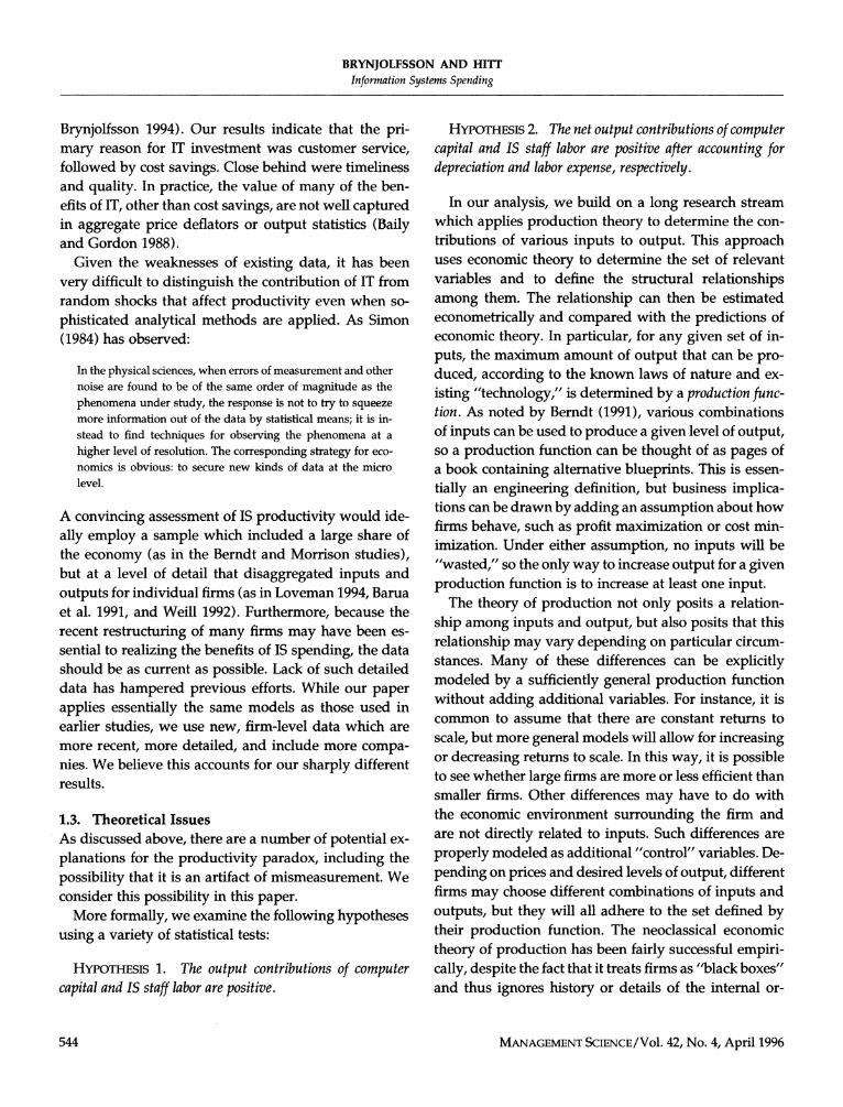
Figure 1 Gross Marginal Product of Computer Capital over Time A second area that can be addressed by our data Marginal Product

200% and method is technology strategy. We have already

18070 found that firms with more computer capital will, cet-

1987 1988 1989 1990 1991

Year

eris paribus, have higher sales than firms with less computer capital, but do the types of computer equip-ment purchased make a difference? We have data on two categories of equipment: (1) central processors, such as mainframes, and (2) PCs and terminals. For this analysis, we divide the sample into three equal groups based on the ratio of central processor value to PCs and terminals. We find that the rate of return

sensitive to sample changes and time-specific exoge-nous events such as the 1991 recession."

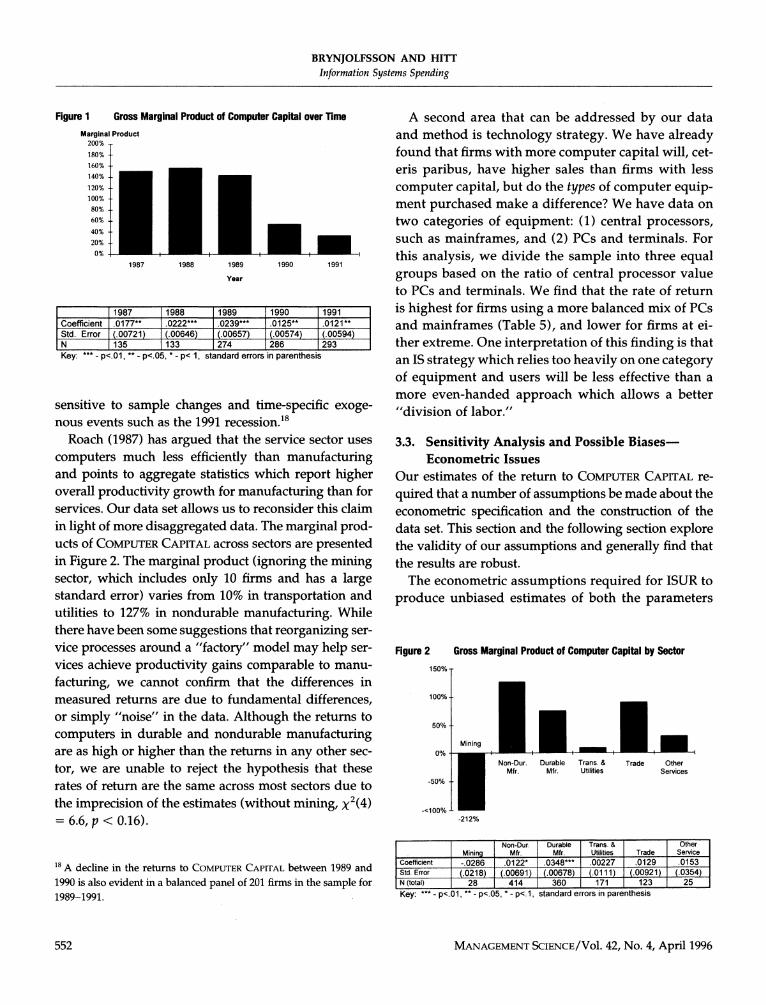
Roach (1987)has argued that the service sector uses computers much less efficiently than manufacturing and points to aggregate statistics which report higher overall productivity growth for manufacturing than for services. Our data set allows us to reconsider this claim in light of more disaggregated data. The marginal prod-ucts of COMPUTERCAPITALacross sectors are presented in Figure 2. The marginal product (ignoring the mining sector, which includes only 10 firms and has a large standard error) varies from 10%in transportation and utilities to 127% in nondurable manufacturing. While there have been some suggestions that reorganizing ser-vice processes around a "factory" model may help ser-vices achieve productivity gains comparable to manu-facturing, we cannot confirm that the differences in measured returns are due to fundamental differences, or simply "noise" in the data. Although the returns to computers in durable and nondurable manufacturing are as high or higher than the returns in any other sec-tor, we are unable to reject the hypothesis that these rates of return are the same across most sectors due to the imprecision of the estimates (without mining, x2(4) = 6.6, p < 0.16).

1987 1988 1989 1990 1991 is highest for firms using a more balanced mix of PCs

l8 A decline in the returns to COMPUTERCAPITALbetween 1989 and 1990 i s also evident ina b a l a n c e d panel of 201 f i rms in the sample for 1989-1991.

of equipment and users will be less effective than a more even-handed approach which allows a better "division of labor."

and mainframes (Table 5), and lower for firms at ei-ther extreme. One interpretation of this finding is that

Coefficient Std Error N

3.3. Sensitivity Analysis and Possible Biases-Econometric Issues

Our estimates of the return to COMPUTERCAPITALre-quired that a number of assumptions be made about the econometric specification and the construction of the data set. This section and the following section explore the validity of our assumptions and generally find that the results are robust.

The econometric assumptions required for ISUR to produce unbiased estimates of both the parameters

Key: *** - p<.01, ** - p<.05, - p< 1, standard errors in parenthesis an IS strategy which relies too heavily on one category

Figure 2 Gross Marginal Product of Computer Capital by Sector

T

.0177=* (.00721) 135

Mfr. Mfr. Utilities Sewlces

-212%

I I 1 Non-Dur I Durable I Trans & I I Other 1

.0222*** (.00646) 133

MANAGEMENTSCIENCE/VOI.42, No. 4, April 1996

.oz3gk** (.00657) 274

Coefficient Std Error N (total)

.0125** (.00574) 286

Key *" - p< 01 *' - pc 05 '- pc 1 standard errors In parenthes~s

Mlnlng

-0286 (0218)

28

.0121** (00594) 293

Mfr 0122'

(00691) 414

Mfr 0348"' (00678)

360

Utliltles 00227

(0111) 171

Trade 0129

(00921) 123

Sewlce

0153 (0354) .

25


Table 5 Split Sample Regression Results-Mainframes as a Percentage of Total Computer Capital

Coefficient Estimates and Marginal Product for Computer Capital Grouping based on mainframes as a percentage of total Computer Capital

Sample Split Highest Middle Lowest Statistical Ordering' Elasticity Estimate (PI) 0.0113** 0.0159*** 0.0117** Standard Error (0.00500) (0.00528) (0.00521) Med > (High, Low) Marginal Product (MPJ 49.1 Oh 79.5% 58.2% ( p < 0.03) Mean O/O Mainframes 74% 54% 34% Group Std. Dev. 9% 5% 8%

Key: ***-p < 0.01, **-p < 0.05, *-p < 0.1, standard errors in parenthesis Ordering by x2tests of return differences. P-value shown represents null hypothesis of equality

across groups.

and the standard errors are similar to those for OLS: additional restrictions on the error structure are not the error term must be uncorrelated with the regres- necessary. Nonetheless, we computed single-year sors (inputs) and homoskedastic in the cross section.I9 OLS estimates both with and without heteroskedas- ISUR implicitly corrects for serial correlation and het- ticity-consistent standard errors to test for heteroske- eroskedasticity over time in our formulation, so that dasticity, and plotted the residuals from the basic

specification to assess normality. These analyses suggest that neither of these assumptions were vio-

l 9 Note that if we had used OLS, further assumptions would be related, although, even if they were coefficient esti- quired: that all error terms are independent and constant variance over

mates (even for OLS), they would still be unbiased time.

and consistent (but standard errors would be in- correct).

However, the assumption that the error term is un-

Table 6 Specification Test-Comparison of OLS and Two-Stage Least correlated with the inputs (orthogonality) is poten- Squares (All parameters (except year dummy) constrained to tially an issue. One way in which this assumption be equal across years) could be violated is if the causality is reversed: in-

stead of increases in purchases of inputs (e.g., com- Parameter OLS Estimates 2SLS Estimates puters) leading to higher output, an increase in out-

p1(Computer Capital) 0.0284*** (0.00723) 0.0435*** (0.0126) put could lead to further investment (for example, a

p2(Noncomputer Capital) 0.0489*** (0.00668) 0.0481* * * (0.00702) firm spends the proceeds from an unexpected in- p3(IS Staff) 0.0191 * * * (0.00795) 0.00727 (0.01 16) crease in demand on more computer equipment). p, (Non-IS Labor and The orthogonality assumption can also be violated if

ExP.1 0.881*** (0.0113) 0.879)*** (0.0125) the input variables are measured with error. The di- Dummy Variables Year*** & Sector*** Year*** & Sector *"

rection of bias of the coefficients from measurement R2 98.3% 98.3% N(total) 702 error is dependent on both the correlation among the 702

variables as well as the correlation among measure- ***-p < 0.01, **-p < 0.05, *-p < 0.1, standard errors are in ment errors (see Kmenta 1986 for a complete dis-

parentheses cussion).'O Note: OLS estimates are for sample of same firms as were available for 2SLS regression (n = 702).

Hausman Test Results (instruments are lagged independent variables): 20 If an input variable is systematically understated by a constant mul- ~ ' ( 4 )= 6.40, ( p < 0.17)-cannot reject exogeneity tiplicative factor, then the coefficient estimates would be unchanged.



Regardless of the source of the error, it is possible to correct for the potential bias using instrumental variables methods, or two-stage least squares (2SLS). We use once-lagged values of variables as instruments, since by definition they cannot be associated with un- anticipated shocks in the dependent variable in the following year." Table 6 reports a comparison of pooled OLS estimates with 2SLS estimates and shows that the coefficient estimates are similar although somewhat higher for COMPUTER and lower for IS STAFF. CAPITAL In both cases the standard errors were substantially larger, as is expected when instrumental variables are used. Using a Hausman specification test, we cannot reject the null hypothesis that the error term is uncorrelated with the regressors (see bottom of Table 5 for test statistics), and therefore do not reject our initial specification.

3.4. Sensitivity Analysis and Possible Biases-Data Issues

To further explore the robustness of our results, we examined the impact of the possible data errors discussed in g2.3 that can be tested: (1) error in the valuation of PCs and terminals, (2) errors in the price deflators, and (3) understatement or misclassification of computer capital.

To assess the sensitivity of the results to possible errors in the valuation of PCs and terminals, we re- calculated the basic regressions varying the assumed average PC and terminal value from $0 to $6K. Note that as the assumed value of PCs and terminals increases, the increase in COMPUTER CAPITALwill be matched by an equal decrease in NONCOMPUTER CAP-ITAL, which is calculated as a residual. Interestingly, the return to COMPUTER in the basic regres- CAPITAL sion is not very sensitive to the assumed value of PCs and terminals, ranging from 77% if they are not counted to 59% if PCs and terminals are counted at $6K (peaking at about 85%).

A second contribution to error is the understatement of output due to errors in the price deflators.

However, in the presence of individual firm effects, lagged values are not valid instruments. While we did not test for firm effects, we suspect they may be important, and so the results of our 2SLS esti-mates should be interpreted with caution.

While it is difficult to directly correct for this problem, we also estimated the basic equations year by year, so that errors in the relative deflators would have no impact on the elasticity estimates. The estimated marginal products ranged from 109% to 197% in the individual year regressions versus 81% when all five years were estimated simultaneously. The standard error on the estimates was significantly higher for all estimates, which can account for the large range of estimates. Overall, this suggests that our basic findings are not a result of the assumed price deflators. However, if the price deflators systematically underestimate the value of intangible product change over time or between firms, our measure of output will be understated, implying that the actual return for computer capital is higher than our estimates.

To assess the third source of error, possible understatement or misclassification of computer capital, we consider three cases: (1) hidden computer spending exists, but does not show up elsewhere in the data; (2) hidden computer spending exists and shows up in the "NoN-IS LABOR AND EXPENSE"category; or (3) hidden computer spending exists and shows up in the "OTHER CAPITAL" category. If the hidden IS costs do not show up elsewhere in the firm (e.g., software de- velopment or training costs from previous years), then the effect on the estimated returns is dependent on how closely correlated these costs are to our measured COMPUTER If they are uncorrelated, CAPITAL. our estimate for the elasticity and the return to COM- PUTER CAPITALis unbiased. If the missing costs are perfectly correlated with the observed costs, then, because of the logarithmic form of our specification, they will result only in a multiplicative scaling of the variables, and the estimated elasticities and the estimated standard error will be unchanged." For the same reason, the sign and statistical significance of our results for the returns to COMPUTER andCAPITAL IS STAFF will also be unaffected. However, the de-

22 This is because multiplicative scaling of a regressor in a logarithmic specification will not change the coefficient estimate or the standard error. All the influence of the multiplier will appear in the intercept term, which is not crucial to our analysis.


BRYNJDLFSSON AND HITT Information Systems Spending

Table 7 Summary of Hypothesis Tests

Hypothesis

H I H I H I H2 H2 H2 H2 H2 Extension of H I Extension of H I Extension of H I

Description of Test (alternative hypothesis)

Positive marginal product for COMPUTER CAPITAL Positive marginal product for IS STAFF Simultaneous test for positive marginal product for COMPUTER and IS STAFF CAPITAL Positive net marginal product for COMPUTER CAPITAL (see Table 6), cost Q 14% (7-year average life) Positive net marginal product for COMPUTER CAPITAL (see Table 6), cost @ 33% (3-year average life) Positive net marginal product for IS STAFF Marginal product of COMPUTER CAPITAL exceeds marginal product of OTHER CAPITAL Marginal product of IS STAFF exceeds marginal product of OTHER LABOR AND EXPENSE Marginal Product of COMPUTER CAPITAL changes across time Marginal Product of COMPUTER CAPITAL varies across sectors Marginal Product varies by mainframes as a percentage of total COMPUTER CAPITAL

Test Statistic

t = 3.92, p < 0.01 t = 3.38, p < 0.01 x2(2) = 43.9, p < 0.01 t = 3.24, p < 0.01 t = 2.32, p < 0.05 x2(1) = 4.4, p < 0.05 See Table 4 x2(1) = 4.0, p < 0.05 x2(4) = 11.2, p < 0.02 x2(4) = 6.6, p < 0.2 x2(2) = 6.9, p < 0.03

nominator used for the MP calculations will be affected by increasing computer capital so the estimated MP will be proportionately lower or higher. For instance, if the hidden costs lead to a doubling of the true costs of computer capital, then the true MP would fall from 81% to just over 40%. Finally, if the hidden costs are negatively correlated with the observed costs, then the true returns would be higher than our estimates.

A second possible case is that hidden IS capital expenses (e.g., software) show up in the NON-IS LABOR AND EXPENSEcategory. To estimate the potential impact of these omissions, we estimate the potential size of the omitted misclassified IS capital relative to COM- PUTER CAPITALusing data from another IDG survey (IDC 1991) on aggregate IS expenditures, including software as well as hardware. To derive a reasonable lower bound on the returns to COMPUTER weCAPITAL, assume that the misclassified IS capital had an average service life of three years, and further make the worst-case assumption of perfect correlation between misclassified IS capital and COMPUTER (andCAPITAL reduce proportionally the amount of NON-IS LABOR AND EXPENSE).In this scenario, our estimates for the amount of COMPUTER in firms roughly dou- CAPITAL bles, yet the rates of return are little unchanged from the basic analysis that does not include misclassified IS capital (68% vs. 81%). This surprising result appears to be due to the fact that the return on NON-IS LABORAND EXPENSEis at least as high as the return

on COMPUTER so moving costs from one cat- CAPITAL, egory to another does not change overall returns much.

Alternatively, a third possible case is that the hidden IS capital expenditures show up in OTHER CAPI-TAL. This would apply to items such as telecommunications hardware, which would normally be classified as a capital expenditure. In this case, the marginal product of COMPUTER CAPITALwill be reduced proportionally to the amount of the misclassification. Intuitively, this case is similar to the case discussed earlier in which the hidden costs are perfectly correlated with measured costs but do not appear elsewhere. Our simulation results indicate that the elasticities on computer capital vary less than 5%even between assumptions of 0% to 100% of computer capital being misclassified.

Irrespective of these sensitivity calculations, it should be noted that the definition of COMPUTER usedCAPITAL in this study was fairly narrow and did not include items such as telecommunications equipment, scientific instruments, or networking equipment. The findings should be interpreted accordingly and do not necessarily apply to broader definitions of IT. However, to the extent that the assumptions of our sensitivity analysis hold, the general finding that IT contributes significantly to output is robust (HI), although the actual point estimates of marginal product may vary, possibly resulting in no statistical difference between returns to computer capital and returns to other capital.



4. Discussion

4.1. Comparison with Earlier Research Although we found that computer capital and IS labor increase output significantly under a variety of formu- lations (see summary Table 7), several other studies have failed to find evidence that IT increases output. Because the models we used were similar to those used by several previous researchers, we attribute our different findings primarily to the larger and more recent data set we used. Specifically, there are at least three reasons why our results may differ from previous results.

First, we examined a later time period (1987-1991) than did Loveman (1978-1982), Barua et al. (1978- 1982), or Berndt and Morrison (1968-1986). The mas- sive build-up of computer capital is a relatively recent phenomenon. Indeed, the delivered amount of com-puter power in the companies in our sample is likely to be at least an order of magnitude greater than that in comparable firms from the period studied by the other authors. Brynjolfsson (1993) argues that even if the MP of IT were twice that of non-IT capital, its impact on output in the 1970s or early 1980s would not have been large enough to be detected with available data by con- ventional estimation procedures. Furthermore, the changes in business processes needed to realize the benefits of IT may have taken some time to implement, so it is possible that the actual returns from investments in computers were initially fairly low. In particular, computers may have initially created organizational slack which was only recently eliminated, perhaps hastened by the increased attention engendered by earlier studies that indicated a potential productivity shortfall and suggestions that "to computerize the office, you have to reinvent the office" (Thurow 1990). Apparently, an analogous period of organizational redesign was necessary to unleash the benefits of electric motors (David 1989).

A pattern of low initial returns is also consistent with the strategy for optimal investment in the presence of learning-by-using: short-term returns should initially be lower than returns for other capital, but subsequently rise to exceed the returns to other capital, compensating for the "investment" in learning (Lester and McCabe 1993). Under this interpretation, our high estimates of computer MP indicate that businesses are beginning to

reap rewards from the experimentation and learning phase in the early 1980s.

Second, we were able to use different and more detailed firm-level data than had been available before. We argue that the effects of computers in increasing variety, quality, or other intangibles are more likely to be detected in firm level data than in the aggregate data. Unfortunately, all such data, including ours, are likely to include data errors. It is possible that the data errors in our sample happened to be more favorable (or less unfavorable) to computers than those in other samples. We attempted to minimize the influence of data errors by cross-checking with other data sources, eliminating outliers, and examining the robustness of the results to different subsamples and specifications. In addition, the large size of our sample should, by the law of large numbers, mitigate the influence of random distur-bances. Indeed, the precision of our estimates was generally much higher than those of previous studies; the statistical significance of our estimates owes as much to the tighter confidence bounds as to higher point estimates.

Third, our sample consisted entirely of relatively large "Fortune 5 0 0 firms. It is possible that the high IS contribution we find is limited to these larger firms. However, an earlier study (Brynjolfsson et al. 1994) found evidence that smaller firms may benefit disproportionately from investments in information technology. In any event, because firms in the sample accounted for a large share of the total U.S. output, the economic relevance of our findings is not heavily dependent on extrapolation of the results to firms outside the sample.

4.2. Managerial Implications If the spending on computers is correlated with significantly higher returns than spending on other types of capital, it does not necessarily follow that companies should increase spending on computers. The firms with high returns and high levels of computer investment may differ systematically from the low performers in ways that cannot be rectified simply by increasing spending. For instance, recent economic theory has sug- gested that "modern manufacturing," involving high intensity of computer usage, may require a radical change in organization (Milgrom and Roberts 1990).



This possibility is emphasized in numerous management books and articles (see, e.g., Malone and Rockart 1991, Scott Morton 1991) and supported in our discus- sions with managers, both at their firms and during a workshop on IT and Productivity attended by approximately 30 industry representative^.^^

Furthermore, our results showing a high gross marginal product may be indicative of the differences between computer investment and other types of investment. For instance, managers may perceive IS investment as riskier than other investments, and therefore require higher expected returns to compensate for the increased risk. Finally, IS is often cited as an enabling technology which does not just produce productivity improvements for individuals, but provides benefits by facilitating business process redesign or improving the ability of groups to work together. In this sense, our results may be indicative of the substantial payoffs to reengineering and other recent business innovations.

5. Conclusion We examined data which included over 1000 observa-tions on output and several inputs at the firm level for 1987-1991. The firms in our sample had aggregate sales of over $1.8 trillion in 1991 and thus account for a sub- stantional share of the U.S. economy. We tested a broad variety of specifications, examined several different subsamples of the data, and validated the assumptions of our econometric procedures to the extent possible. Overall, we found that computers contribute significantly to firm-level output, even after accounting for depreciation, measurement error, and some data limita- tions.

There are a number of other directions in which this work could be extended. First, the data set could be ex- panded to include alternative measures of output, such as value added, and to include additional inputs, such as R&D, that have been explored in other literature (see Brynjolfsson and Hitt 1995). Second, although our ap-

proach us to infer the created intan-gibles like product variety by looking at changes in the

23 The MIT Center for Coordination Science and International Financial Services Research Center jointly sponsored a Workshop on IT and Pro- ductivity which was held in December, 1992.


revenues at the firm level, more direct approaches might also be promising such as directly accounting for intangible outputs such as product quality or variety.

Finally, the type of extension which is likely to have the greatest impact on practice is further analysis of the factors which differentiate firms with high returns to IT from low performers. For instance, is the current "downsizing" of firms leading to higher IT productivity? Are the firms that have undertaken substantial "reengineering efforts" also the ones with the highest returns? Since this study has presented evidence that the computer "productivity paradox" is a thing of the past, it seems appropriate that the next round of work should focus on identifying the strategies which have led to large IT prod~ct ivi ty .~~

24 This research has been generously supported by the MIT Center for Coordination Science, the MIT Industrial Performance Center, and the MIT International Financial Services Research Center. We thank Mar- tin Neil Baily, Rajiv Banker, Ernst Berndt, Geoff Brooke, Zvi Griliches, Bronwyn Hall, Susan Humphrey, Dan Sichel, Robert Solow, Paul Strassmann, Diane Wilson, three anonymous referees, and seminar participants at Boston University, Citibank, Harvard Business School, the International Conference on Information Systems, MIT, National Technical University in Singapore, Stanford University, the University of California at Irvine, and the U.S. Federal Reserve for valuable com- ments, while retaining responsibility for any errors that remain. We are also grateful to International Data Group for providing essential data. An earlier, abbreviated version of this paper was published in the Proceedings of the International Conference on Information Systems, 1993, under the title "Is Information Systems Spending Productive? New Evidence and New Results."

References Baily, M. N. and R. J. Gordon, 'The Productivity Slowdown, Mea-

surement Issues, and the Explosion of Computer Power," in W. C. Brainard and G. L. Perry (Eds.), Brookings Papers on Eco- nomic Activity, The Brookings Institution, Washington, DC, 1988.

Bama, A,, C. Kriebel, and T. Mukhopadhyay, "Information Technol- ogy and Business Value: An Analytic and Empirical Investiga- tion," University of Texas at Austin Worlang Paper, Austin, TX, May, 1991.

Berndt, E., The Practice of Econometrics: Classic and Contemporary, Ad-dison-Wesley, Reading, MA, 1991.

Brynjolfsson, E., "The Productivity Paradox of Information Technol-

ogy," comm. ACM, 35 (1993), 66-77. -,"Technology's True Payoff," Informationweek (October 10,1994),

34-36. -and L. Hitt, "Is Information Systems Spending Productive? New

Evidence and New Results," Proc. 14th International Conf. on In- formation Systems, Orlando, FL,1993.


Brynjolfsson, E, and L. Hitt, "Information Technology as a Factor of Production: The Role of Differences Among Firms," Economics of Innovation and New Technology, 3,4 (1995), 183-200.

-, T. Malone, V. Gurbaxani, and A. Kambil, "Does Information Technology Lead to Smaller Firms?', Management Sci., 40, 12 (1994).

Bureau of Economic Analysis, U. S. D. o. C., Fixed Reproducible Tangible Wealth In the United States, 1925-85, U.S. Government Printing Office, Washington, DC, 1987.

Christensen, L. R., and D. W. Jorgenson, "The Measurement of U.S. Real Capital Input, 1929-1967," Review of Income and Wealth, 15, 4 (1969), 293-320.

Dos Santos, B. L., K. G. Peffers, and D. C. Mauer, "The Impact of Information Technology Investment Announcements on the Mar- ket Value of the Firm," Information Systems Res., 4 , l (1993), 1-23.

Harris, S. E, and J. L. Katz, "Profitability and Information Technology Capital Intensity in the Insurance Industry," in Proc. Twenty-Flrst Hawaii International Conf. on System Science, 1988.

International Data Corporation (IDC), "U.S. Information Technology Spending Patterns, 1969-1994," IDC Special Report 5368,1991.

Kmenta, J., Elements of Econometrics, Second edition, Macmillan, New York, 1986.

Loveman, G. W., "An Assessment of the Productivity Impact on In- formation Technologies," in T. J. Allen and M. S. Scott Morton (Eds.),Information Technology and the Corporation of the 1990s: Re-search Studies, MIT Press, Cambridge, MA, 1994.

Malone, T., and J. Rockart, "Computers, Networks and the Corpora- tion," Scientific Amencan, 265, 3 (1991), 128-136.

Accepted by John C. Henderson; received November 1993; this paper has been

Milgrom, P. and J. Roberts, "The Economics of Modern Manufactur- ing: Technology, Strategy, and Organization," American Economic Rev., 80,3 (1990), 511-528.

Morrison, C. J. and E. R. Berndt, "Assessing the Productivity of Infor- mation Technology Equipment in the U.S. Manufacturing Indus- tries," National Bureau of Economic Research Working Paper 3582, January, 1990.

Pelaia, E., "IBM Terminal Prices," personal communication with IBM Representative, 1993.

Popkin, J., and Company, "The Impact of Measurement and Analytical Issues in Assessing Industry Productivity and its Relation to Computer Investment," Washington, DC, Mimeo October, 1992.

Quinn, M. A. et al., "Critical Issues of Information Systems Manage- ment for 1993," CSC Index, The Sixth Annual Survey of Infor- mation Systems Management Issues, Cambridge, MA, 1993.

Scott Morton, M. (Ed.), The Corporation of the 1990s: Information Tech- nology and Organizational Transformation, Oxford University Press, New York, 1991.

Strassmann, P. A,, The Business Value of Computers, Information Eco- nomics Press, New Canaan, CT, 1990.

Thurow, L., "Are Investments in Information Systems Paying Off?," MIT Management Spring (1990).

Varian, H., Microeconomic Analysis, Third Edition, W. W. Norton & Company, Inc., New York, 1992.

Wilson, D., "Assessing the Impact of Information Technology on Or- ganizational Performance," in R. Barker, R. Kauffman, and M. A. Mahmood (Eds.), Strategic Information Technology Management, Idea Group, Harrisburg, PA, 1993.

with the authors 12 months for 3 revisions.


Paradox Lost? Firm-level Evidence on the Returns to Information

Documents

Transcript of Paradox Lost? Firm-level Evidence on the Returns to Information