Paper SAS3080-2016 Holiday Demand Forecasting...

1

Paper SAS3080-2016

Holiday Demand Forecasting in the Electric Utility Industry

Jingrui Xie and Alex Chien, SAS Institute Inc.

ABSTRACT

Electric load forecasting is a complex problem that is linked with social activity considerations and variations in weather and climate. Furthermore, electricity is one of only a few goods that has almost no inventory. The absence of inventory means that electric utilities’ operations depend heavily on accurate load forecasts to balance the demand and supply in an almost real-time fashion. This electric load forecasting problem is even more challenging for holidays, which have limited historical data and varying demand patterns. These challenges result in the forecast error for holidays being higher, on average, than it is for regular days. This paper investigates three practical holiday electric demand forecasting techniques: modeling holidays as weekends, modeling holidays using holiday dummy variables, and a two-stage method in which the second stage models residuals. The empirical results from this investigation show that the selection of holiday electric demand forecasting strategy depends both on the holiday itself and on the availability of the historical data.

INTRODUCTION

Electric utilities use load forecasts for different purposes including energy trading [1], system operation and planning [2], and demand-side management [3]. Demand forecasting for electric utilities is different from that for other industries such as retail and airline passengers because electricity is a special type of goods that cannot be widely stored to meet the demand when there is a need. This means that electric utilities’ operations depend heavily on accurate load forecasts to balance the demand and supply in an almost real-time fashion. The electric demand forecasting for holidays is even more challenging because of the limited sample data size and the varying load profiles across different holidays or across the same holiday in different years.

Extensive research has been done on holiday electric demand forecasting. In most cases, holidays were modeled simply as different weekday groups or as weekend days. Song et al. applied fuzzy linear regression on holiday load forecasting, which grouped holidays based on the weekday they fell on [4]. Holidays were treated as weekends in [5]–[7], although different modeling techniques were applied. In some other cases, researchers followed more complicated modeling steps for modeling holidays. For example, Khotanzad and Afkhami-Rohani [8] used a two-stage method for holiday electric demand forecasting. In the first stage, the holiday electric demand was forecasted according to the weekday it fell on and the peak load of the holiday was forecasted by using demand series with a similar temperature profile. In the second stage, the holiday electric demand forecasts were reshaped based on the peak load forecasts. Xie and Hong [9] also followed a two-stage approach for electric demand forecasting including holidays, where the second stage modeled the residuals.

This paper evaluates three practical holiday electric demand forecasting techniques: (1) treating holidays as weekend days, (2) using holiday dummy variables, and (3) a two-stage method in which the second stage models the residuals. This paper also investigates how the availability of historical information affects the selection of the holiday electric demand forecasting technique.

BACKGROUND

DATA

The data being used for this study are the system demand data from ISO New England.1 The data include 10 years (2004–2013) of hourly load and temperature data. This paper uses system demand for holidays in the last five years (2009–2013) for out-of-sample tests. For example, first the hourly demand for holidays in 2009 is forecasted with the previous five years (2004–2008) being used as training data. Then, the forecast origin is moved forward to forecast the hourly demand for holidays in 2010 with the previous five

1 http://www.iso-ne.com/

http://www.iso-ne.com/

2

years (2005–2009) being used as training data. This process is repeated until forecasts for all five years from 2009 to 2013 are generated. In total, 10 US Federal holidays listed in Table 1 are considered.

Holiday Date

1 New Year’s Day January 1

2 Birthday of Martin Luther King Jr. Third Monday in January

3 Washington’s Birthday Third Monday in February

4 Memorial Day Last Monday in May

5 Independence Day July 4

6 Labor Day First Monday in September

7 Columbus Day Second Monday in October

8 Veterans Day November 11

9 Thanksgiving Fourth Thursday in November

10 Christmas Day December 25

Table 1. Ten US Federal Holidays

Figure 1 presents the hourly demand on each of the 10 holidays for the five years from 2004 to 2008. Each holiday has a unique demand pattern, and the demand patterns of the same holiday also vary across different years.

Figure 1. Hourly Electric Demand of 10 US Federal Holidays

BENCHMARK MODEL

Multiple linear regression (MLR) models have been widely used for load forecasting [7], [10], [11]. Because of its simplicity, transparent, and popularity, the MLR model is also used for this study. Among the various MLR models, Tao’s Vanilla Benchmark model and its variations [7] have been widely adopted [1], [2], [9]–[12]. This paper follows the model selection process proposed in [7] to account for the recency effect in load forecasting (that is, using one or more lags of the temperature), leading to the benchmark model as defined in the following equation with i = 0, 1, 2, and 3:

3

0 1 2 3 4 5

( ) ( ) t t t t t t t t i ti

Load Trend M W H W H f T f T

242 3 2 3

1 2 3 4 5 6 1

1 where ( ) and

24t i t i t t i t t i t t i t t i t t i t t t hh

f T T M T M T M T H T H T H T T

In this equation, Ht , Wt, and Mt are CLASS variables that represent the hour of the day, the day of the week, and the month of the year, respectively; Tt-i is the temperature of the current hour or the previous ith hour; and Trendt is a chronological trend.

Mean absolute percentage error (MAPE) has been widely used for evaluating the forecasting performance. In this paper, the average value of the MAPEs for forecasting each holiday in the five test years is used to compare the performance of different holiday electric demand techniques.

This paper uses the GLM procedure in SAS/STAT® software for building the MLR models. For information about PROC GLM, see the chapter “The GLM Procedure” in SAS/STAT User’s Guide. The following code uses the benchmark model to generate the forecasts:

proc glm data=inputData noprint;

class month weekday hour;

model load = trend weekday*hour

t0*month t0*t0*month t0*t0*t0*month

t0*hour t0*t0*hour t0*t0*t0*hour







ta*month ta*ta*month ta*ta*ta*month

ta*hour ta*ta*hour ta*ta*ta*hour

/SS1 SS3 SOLUTION SINGULAR=1E-07;

output out=forecastResults predicted=predict;

run;

quit;

MODELING HOLIDAY ELECTRIC DEMAND

MODELING HOLIDAYS AS WEEKENDS

The rationale for modeling holidays as weekends is that human activities during holidays are similar to their activities during weekends. Modeling holidays as weekends can help tackle the challenge of limited history data. This paper models holidays both as Saturday and as Sunday, and then selects the model that has the lowest average MAPE. For year j (j = 2009, …, 2013), first the data for days other than holidays for the previous five years’ (years j–1, ..., j–5) are used to estimate the coefficients of the benchmark model. Then, the estimated coefficients are used to score the input data of year j for all the holidays, with each holiday being considered as Saturday or Sunday. The estimated coefficients are also used to score the input data of holidays in the training data years (years j–1, …, j–5), with those holidays also being considered as weekends in order to derive the forecast residuals. In this paper, the residuals are defined as the actual values minus the forecasted values and are discussed further in the section “Two-Stage Modeling.”

The following DATA step treats the holiday as a weekend day. The macro variable holiday_i takes a value from 1 to 10 to represent one of the holidays, and the macro variable weekend takes the value of 1 or 7 to represent treating the holiday as Sunday or Saturday. These preprocessed input data are then used in the benchmark model.

4

data inputData;

set inputData;

if holiday = &holiday_i then weekday = &weekend;

where holiday in(0, &holiday_i);

run;

MODELING HOLIDAYS USING DUMMY VARIABLES

Dummy variables (which have a value of 0 or 1 to represent an attribute that has two distinct categories) have been widely used in regression analysis. Dummy variables can be created for normal days of the week and for each of the 10 holidays, and added to the benchmark model to represent whether a day is a holiday or not.To do so, a new variable, Holiday, is specified as a CLASS variable in the GLM procedure. A value of 0 for Holiday indicates that the day is not a holiday; values 1 through 10 indicate that the day is one of the 10 holidays. Because Holiday is a CLASS variable, the GLM procedure automatically creates 10 dummy variables to indicate whether a day is one of the 10 holidays. The following code shows the benchmark model with the CLASS variable Holiday:


class month weekday hour holiday;

model load = trend weekday*hour holiday













run;

quit;

Figure 2 shows the scatter plots of hourly load versus hourly temperature by hour of the day in the year 2008. This paper presents data only from year 2008 because other years show similar patterns. The scatter plots suggest that electric demand series respond to temperature significantly differently during different hours of the day. Thus, in addition to using Holiday as CLASS variable by itself, using the interaction between the CLASS variables Holiday and Hour of the day is also evaluated.

5

Figure 2. Electric Demand by Hour of Day (Year = 2008)

The following code shows the benchmark model with the CLASS variable Holiday and its interaction with the CLASS variable Hour:


class month weekday hour holiday;

model load = trend weekday*hour holiday*hour













run;

quit;

TWO-STAGE MODELING

Residuals account for everything else that is not explained by the model. Research has been done to analyze residuals in order to further improve the forecast [7], [12]. Figure 3 through Figure 5 present the residuals from scoring the holidays in the training periods by using the benchmark model with and without treating holidays as a weekend day. Consistent patterns are evident in the residuals for the holiday load forecasts. For example, when holiday 9 (Thanksgiving) is treated as a weekend day, the demand is always underestimated during the morning period and overestimated during the afternoon period, because people cook earlier than usual on Thanksgiving, which causes a higher morning peak. This pattern is opposite the pattern for other weekdays or weekend days.

6

Figure 3. Residuals of Benchmark Model without Treating Holiday as a Weekend Day

Figure 4. Residual of Benchmark Model by Treating Holidays as Saturday

7

Figure 5. Residual of Benchmark Model by Treating Holidays as Sunday

This paper proposes a two-stage method: During the first stage, the holiday demand is forecasted using the benchmark model with and without treating holidays as weekend days. During the second stage, the average of the residuals from the scored training data is calculated by holiday and by hour. The averaged residual is then added by holiday and by hour to the stage-one load forecasts to yield the final two-stage forecast results. The code for the first stage has been discussed in previous sections; the following code shows how to calculate the average of residuals and add it back to the forecasted load from stage one:

data stageOneResults

FitResults;

set forecastResults;

e = sum(actual,-predict);

if year=%eval(&fcst_year) then output stageOneResults;

else output FitResults;

run;

proc sort data= FitResults out=sort_holiday_hour;

by holiday hour;

run;

proc means data=sort_holiday_hour noprint;

by holiday hour;

var e;

output out=avg_residual_holiday_hour;

run;

data avg_residual_holiday_hour;

set avg_residual_holiday_hour;

8

where _stat_ = "MEAN";

run;

proc sql;

create table stageTwoResults as

select t1.*, t2.e as avg_residual,

sum(t1.predict, t2.e) as predict_2s

from stageOneResults as t1, avg_residual_holiday_hour as t2

where t1.holiday = t2.holiday and t1.hour = t2.hour;

quit;

RESULTS

Figure 6 presents the average MAPE of the five test years for each holiday from the following various holiday electric demand forecasting techniques:

benchmark model (black line with dot marker labeled No treatment)

benchmark model with holidays being modeled as a weekend day (blue line with cross marker labeled As Weekend)

benchmark model with Holiday as a CLASS variable (purple line with triangle marker labeled Holiday)

benchmark model with the CLASS variable Holiday and the CLASS variable Hour of the Day interaction (green line with diamond marker labeled Holiday*Hour)

two-stage approach (red line with star marker labeled Residual)

Figure 6. MAPEs of Holiday Demand Forecasts from Different Holiday Demand Modeling Techniques

(Five Years of Training Data)

The results show that no single holiday demand modeling technique dominates all others, but the proposed two-stage method performs well in most cases. For holidays 1, 4, 5, and 10, the differences between the proposed method and the benchmark model with holidays being modeled as a weekend day are negligible. Compared with the benchmark model, using Holiday as a CLASS variable better captures the holiday electric usage pattern. However, using the interaction of the CLASS variables Holiday and Hour of the day further improves the MAPE. Using the interaction of these two CLASS variables also provides results that are almost as good as the results of applying the two-stage method.

9

DISCUSSION

MODELING THE RESIDUALS USING THE GRADIENT BOOSTING MODEL

The proposed idea of taking the average of the residuals of the scored historical holiday samples is only one way to model the residuals. It assumes that the models have stable holiday forecast residuals from time to time. Another way to model the residuals is by using the gradient boosting model (GBM), which builds the model in a stagewise fashion. In the first step, the GBM builds a model for the predictor (electric demand in this paper). Then it improves the model by building a new model that adds the prediction of the residuals to the original model.

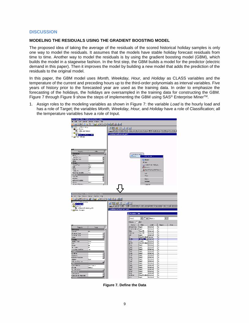
In this paper, the GBM model uses Month, Weekday, Hour, and Holiday as CLASS variables and the temperature of the current and preceding hours up to the third-order polynomials as interval variables. Five years of history prior to the forecasted year are used as the training data. In order to emphasize the forecasting of the holidays, the holidays are oversampled in the training data for constructing the GBM. Figure 7 through Figure 9 show the steps of implementing the GBM using SAS® Enterprise MinerTM.

1. Assign roles to the modeling variables as shown in Figure 7: the variable Load is the hourly load and has a role of Target; the variables Month, Weekday, Hour, and Holiday have a role of Classification; all the temperature variables have a role of Input.

Figure 7. Define the Data

10

2. Drag the Gradient Boosting icon (on the Model tab) to the workspace and connect it with the data node, as shown in Figure 8.

Figure 8. Create a Gradient Boosting Model

3. Adjust the default values of parameters for the gradient boosting model as highlighted in Figure 9.

Figure 9. Adjust the Parameters

11

4. Click the Run icon to execute the gradient boosting model as shown in Figure 10.

Figure 10. Execute the Gradient Boosting Model

Figure 11 presents the MAPE of each holiday from the benchmark model, the GBM, and the proposed two-stage modeling method. Although the GBM achieves remarkable improvements for holiday load forecasting, the proposed two-stage method still outperforms the GBM in most cases. However, this study might shed light on future research into using the GBM to investigate the oversampling strategy in order to further improve demand forecasting during rare events.

Figure 11. MAPEs of Holiday Demand Forecasts from Different Holiday Demand Modeling Techniques

(Five Years of Training Data)

IMPACT OF THE AVAILABILITY OF HISTORICAL DATA

Table 2 shows the average MAPE of the five test years for each holiday from using different timespans of training data. The cooler the color of the cell, the lower the MAPE. When the historical data are sufficient, both the two-stage model and using the interaction of Holiday and Hour of the Day CLASS variables perform well. As the historical data become limited, using holiday dummy variables becomes less reliable. When the historical data are extremely limited (for example, only one year of history is available), treating holidays as weekend days might help in some cases; but in most cases, any advanced holiday modeling technique might not outperform the simple benchmark model. In summary, not only does the choice of the holiday modeling technique vary from one holiday to another, but the choice is also affected by the availability of historical data for modeling.

12

Training

Data Length Holiday

No

Treatment

As

Weekend Holiday Holiday*Hour Residuals

5 y

ears

1 9.84% 3.36% 6.46% 3.10% 3.09%

2 2.59% 6.48% 2.22% 1.69% 1.71%

3 4.63% 4.97% 3.14% 1.82% 1.87%

4 10.03% 3.87% 7.92% 3.98% 3.81%

5 10.12% 3.09% 5.98% 4.09% 3.35%

6 8.01% 4.22% 7.38% 4.59% 3.87%

7 5.28% 5.69% 3.26% 2.58% 2.29%

8 2.66% 8.07% 2.26% 2.01% 2.02%

9 14.07% 6.13% 8.65% 3.05% 3.05%

10 10.73% 3.66% 6.49% 3.45% 3.47%

3 y

ears

1 9.54% 3.33% 6.46% 3.56% 3.61%

2 2.69% 6.48% 2.24% 1.97% 1.81%

3 4.50% 4.97% 3.04% 2.02% 2.08%

4 10.02% 3.86% 7.55% 3.91% 3.75%

5 9.64% 3.30% 6.52% 4.91% 4.05%

6 7.78% 3.79% 6.64% 4.00% 3.09%

7 4.97% 6.08% 3.01% 2.56% 2.32%

8 2.72% 8.33% 2.48% 2.40% 2.44%

9 13.86% 6.22% 8.50% 2.79% 2.72%

10 10.65% 4.25% 6.97% 4.43% 4.18%

1 y

ears

1 7.80% 7.82% 9.27% 8.72% 8.72%

2 6.75% 12.03% 6.85% 7.06% 7.09%

3 6.37% 10.55% 7.18% 6.71% 6.82%

4 8.08% 8.48% 10.99% 9.93% 10.04%

5 14.09% 14.22% 17.88% 18.32% 18.39%

6 8.21% 9.60% 12.18% 11.24% 11.35%

7 6.97% 12.11% 8.46% 8.39% 8.44%

8 7.72% 15.33% 7.93% 8.18% 8.08%

9 10.59% 8.70% 11.31% 8.83% 8.94%

10 7.42% 6.95% 10.12% 9.06% 9.07%

Table 2. MAPE Values of Using Different Timespans of Training Data from Different Modeling Techniques

CONCLUSION

This paper investigates three practical techniques for holiday electric demand forecasting. The results show that different holidays might require different holiday modeling techniques and that the two-stage method performs well in many cases. Furthermore, the paper demonstrates that the selection of holiday load forecasting strategy also depends highly on the availability of training data.

13

REFERENCES

[1] Xie, J., Hong, T., and Stroud, J. (2015). “Long-Term Retail Energy Forecasting with Consideration of Residential Customer Attrition.” IEEE Transactions on Smart Grid 6:2245–2252.

[2] Hong, T., Wilson, J., and Xie, J. (2014). “Long Term Probabilistic Load Forecasting and Normalization with Hourly Information.” IEEE Transactions on Smart Grid 5:456–462.

[3] Hong, T., and Wang, P. (2012). “On the Impact of Demand Response: Load Shedding, Energy Conservation, and Further Implications to Load Forecasting.” IEEE Power and Energy Society General Meeting, San Diego, 2–4.

[4] Song, K., Baek, Y., Hong, D. H., and Jang, G. (2005). “Short-Term Load Forecasting for the Holidays Using Fuzzy Linear Regression Method.” IEEE Transactions on Power Systems 20:96–101.

[5] Rahman, S., and Bhatnagar, R. (1988). “An Expert System Based Algorithm for Short Term Load Forecast.” IEEE Transactions on Power Systems 3:392–399.

[6] Krogh, B., de Llinas, E. S., and Lesser, D. (1982). “Design and Implementation of an On-line Load Forecasting Algorithm.” IEEE Transactions on Power Apparatus and Systems PAS-101:3284–3289.

[7] Hong, T. (2010). “Short Term Electric Load Forecasting.” Ph.D. diss., Graduate Program of Operations Research and Department of Electrical and Computer Engineering, North Carolina State University.

[8] Khotanzad, A., and Afkhami-Rohani, R. (1998). “ANNSTLF—Artificial Neural Network Short-Term Load Forecaster, Generation Three.” IEEE Transactions on Power Systems 13:1413–1422.

[9] Xie, J., and Hong, T. (2015). “GEFCom2014 Probabilistic Electric Load Forecasting: An Integrated Solution with Forecast Combination and Residual Simulation.” International Journal of Forecasting, December. Available online: DOI: 10.1016/j.ijforecast.2015.11.005.

[10] Black, J. D., and Henson, W. L. W. (2014). “Hierarchical Load Hindcasting Using Reanalysis Weather.” IEEE Transactions on Smart Grid 5:447–455.

[11] Hoverstad, B. A., Tidemann, A., Langseth, H., and Ozturk, P. (2015). “Short-Term Load Forecasting with Seasonal Decomposition Using Evolution for Parameter Tuning.” IEEE Transactions on Smart Grid 6:1904–1913.

[12] Xie, J., Hong, T., Laing, T., and Kang, C. (2015). “On Normality Assumption in Residual Simulation for Probabilistic Load Forecasting.” IEEE Transactions on Smart Grid PP:1.

CONTACT INFORMATION

Your comments and questions are valued and encouraged. Contact the authors:

Jingrui Xie SAS Campus Drive Cary, NC 27513 919-531-1628 [email protected] Alex Chien SAS Campus Drive Cary, NC 27513 919-531-9236 [email protected]

SAS and all other SAS Institute Inc. product or service names are registered trademarks or trademarks of SAS Institute Inc. in the USA and other countries. ® indicates USA registration.

Other brand and product names are trademarks of their respective companies.

mailto:[email protected]

mailto:[email protected]

Paper SAS3080-2016 Holiday Demand Forecasting...

Documents

Transcript of Paper SAS3080-2016 Holiday Demand Forecasting...