IEICE TRANS. COMMUN., VOL.E93–B, NO.10 OCTOBER 20102611

PAPER Special Section on Advanced Technologies in Antennas and Propagation in Conjunction with Main Topics of ISAP2009

Quantitative Evaluation for Computational Cost of CG-FMM onTypical Wiregrid Models

Keisuke KONNO†a), Student Member, Qiang CHEN†, Member, and Kunio SAWAYA†, Fellow

SUMMARY The conjugate gradient-fast multipole method (CG-FMM)is one of the powerful methods for analysis of large-scale electromagneticproblems. It is also known that CPU time and computer memory can be re-duced by CG-FMM but such computational cost of CG-FMM depends onshape and electrical properties of an analysis model. In this paper, relationbetween the number of multipoles and number of segments in each groupis derived from dimension of segment arrangement in four typical wiregridmodels. Based on the relation and numerical results for these typical mod-els, the CPU time per iteration and computer memory are quantitativelydiscussed. In addition, the number of iteration steps, which is related tocondition number of impedance matrix and analysis model, is also consid-ered from a physical point of view.key words: Method of Moments (MoM), conjugate gradient, fast multipolemethod

1. Introduction

The Method of Moments (MoM) is one of the powerfultechniques for numerical analysis of antennas and scatter-ers [1], [2]. However, CPU time and computer memory tosolve matrix equation in MoM by using conventional di-rect methods such as Gaussian elimination are proportionalto O(N3) and O(N2), respectively, where N is the numberof unknowns. Even though powerful computers with largememories are available, it is impossible to solve large-scaleproblems with millions of unknowns by the direct methods.Therefore, many techniques have been developed to reducethe CPU time and computer memory of MoM computation.

Iterative method such as the Conjugate Gradient (CG)method has been used to solve the MoM matrix equation inprevious studies [3]–[8]. Unlike direct methods, the CPUtime to solve the matrix equation by CG method is deter-mined by number of iteration steps and CPU time per iter-ation. Therefore, computational cost of CG method is clas-sified into three factors, i.e., the number of iteration steps,CPU time per iteration, and the computer memory. Thenumber of iteration steps depends on the analysis model,while the CPU time per iteration and computer memory ofCG method are both the order of O(N2).

In above three factors, the number of iteration stepsof CG method has been discussed in a few papers sofar and it has been reported that the number of iterationsteps is strongly depended on the condition number of the

Manuscript received January 4, 2010.Manuscript revised May 4, 2010.†The authors are with the Department of Electrical Commu-

nications Engineering, Graduate School of Engineering, TohokuUniversity, Sendai-shi, 980-8579 Japan.

a) E-mail: konno@ecei.tohoku.ac.jpDOI: 10.1587/transcom.E93.B.2611

impedance matrix Z [6]–[8]. But in these papers, little at-tention is paid to relation between the number of iterationsteps and analysis model, as well as relation between condi-tion number of Z and analysis model.

On the other hand, it is known that other two fac-tors except the number of iteration steps, namely, the CPUtime per iteration and computer memory of CG method canbe reduced by the Fast Multipole Method (FMM) [9], [10]or Multi-Level Fast Multipole Algorithm (MLFMA) [11]–[20]. It has been considered that the CPU time per iterationand computer memory of CG method combined with FMM(CG-FMM) are both O(N1.5). However, the CPU time per it-eration and computer memory in CG-FMM depend on manyparameters for FMM as well as analysis model. Choice ofparameters such as the number of multipoles or a group sizefor the two and three dimensional FMM have been discussedin a few papers [21], [22]. However, parameter choice basedon these papers are not always correct in general since shapeof analysis model, which is highly related to the number ofmultipoles L, has not been considered in these papers.

In this paper, four typical wiregrid models, which isformed electrically continuous or separated geometry, andone-dimensional or two-dimensional geometry, are intro-duced. It is shown that relation between the number of mul-tipoles L and number of segments in each group K is deter-mined by dimension of segment arrangement in an analysismodel, and the relation is used to discuss not only the CPUtime per iteration but also the computer memory requiredfor analysis. Based on numerical simulation for these typ-ical models, mutual relation among the number of iterationsteps, condition number of Z and analysis model can be dis-cussed universally from a physical point of view.

This paper is organized as follows. Section 2 presentsprinciple of CG-FMM and important parameters related tothe computational cost. In Sect. 3, four typical models andtwo different relations between L and K are shown. InSect. 4, the computational cost of CG-FMM for these typ-ical models is discussed theoretically and numerically.

2. Principle of CG-FMM

2.1 Conjugate Gradient Method

Matrix equation produced by the MoM is expressed by

ZI = V, (1)

where Z is N × N impedance matrix produced by the MoM,

Copyright© 2010 The Institute of Electronics, Information and Communication Engineers

2612IEICE TRANS. COMMUN., VOL.E93–B, NO.10 OCTOBER 2010

V is N-dimensional known voltage vector, and I is N-dimensional unknown current vector. The algorithm of CGmethod for solving Eq. (1) is summarized as follows [3]–[8].

CG method for MoM.

• After initial value of I is set to be I0, initial value ofresidual vector R0 and correction vector for solutionP0 are calculated as

R0 = V − ZI0,

P0 = Z†R0.

• Iterations (i = 1, 2, ...) are stopped after the desiredresidual norm ‖Ri‖ is obtained as

αi =〈ZPi−1,Ri−1〉‖ZPi−1‖2

=

∥∥∥Z†Ri−1

∥∥∥2‖ZPi−1‖2

,

Ii = Ii−1 + αiPi−1,

Ri = V − ZIi = Ri−1 − αiZPi−1.

If ‖Ri‖ < ε ‖V‖ , iteration is stopped.

βi =

∥∥∥Z†Ri

∥∥∥2∥∥∥Z†Ri−1

∥∥∥2 ,Pi = Z†Ri + βiPi−1,

where αi and βi are correction coefficients for Ii−1 and Pi−1,respectively, and ε is an error control parameter for the so-lution. Z† denotes the conjugate transpose of Z.

In the above algorithm, two times of matrix-vectormultiplication are carried out in each iteration and CPU timefor the matrix-vector multipication is O(N2). In addition,computer memory for storing Z is also O(N2).

2.2 Fast Multipole Method

FMM is a method based on the addition theorem of thescalar Green’s function [9], [10]. FMM can reduce both theCPU time for the matrix-vector multiplication and computermemory of CG method to O(N1.5) when number of groupsM =

√N. The matrix-vector multiplication in each step

of CG-FMM can be collectively carried out by groupingscheme based on the addition theorem. In addition, mu-tual impedance between far segments are calculated by theaddition theorem at every time of the matrix-vector multipli-cation in CG-FMM and the full impedance matrix Z is notnecessary to be stored. In what follows, formulation of themutual impedance between far segments based on FMM isexplained.

In the Galerkin-MoM, the expression of the mutualimpedance between far segments is obtained as

Zfarmkm′k′ = jωμ0

∫lmk

fmk(rk)

·∫

lm′k′G0(rk, rk′) · fm′k′(rk′)dr′dr, (2)

Fig. 1 Definition of vectors and subscripts for FMM formulation.

where m and m′(= 1, 2, ...,M) are observation group num-ber and source group number, respectively [1]. k and k′(=1, 2, ...,N/M(= K)) represent segment number in mth obser-vation group and m′th source group, respectively. Here, Mis the total number of groups and K is the total number ofsegments in each group. lmk and lm′k′ denote the path of inte-gration along the observation segment and source segment.Figure 1 shows the definition of vectors and subscripts.

When |rmm′ | � |rm′k′ − rmk|, the Gegenbauer’s additiontheorem [23] and plane wave expansion for spherical wavescan be applied to Eq. (2) and

Zfarmkm′k′ ≈

ωμ0k0

(4π)2

∫ 2π

0

∫ π0

smk(k)Tmm′s∗m′k′(k) sin θdθdφ, (3)

is obtained, where smk(k), sm′k′(k), and Tmm′ are expressedas follows.

smk(k) =∫

lmk

e jk·rmk (I − kk) · fmk(rk)drk. (4)

sm′k′(k) =∫

lm′k′e jk·rm′k′ (I − kk) · fm′k′(rk′)drk′ . (5)

Tmm′ =

L∑l=0

(− j)l(2l + 1)h(2)l (k0rmm′)Pl(k · rmm′). (6)

smk(k), called “receiving function” means the mutualimpedance between the center of the mth observation groupand kth segment in mth group. sm′k′(k), called “radia-tion function” means the mutual impedance between thecenter of the m′th source group and k′th segment in m′thgroup. Tmm′ , called “transfer function” represents the mu-tual impedance between the center of the mth observation

group and that of the m′th source group. I = xx + yy + zzdenotes the unit dyad and k = x sin θ cosφ + y sin θ sinφ +z cos θ is an unit vector of radial direction on an unit sphere.h(2)

l is the lth order spherical Hankel function of the secondkind and Pl is the Legendre polynomial of lth order.

Equation (6) is a finite series whose summation is trun-cated at L. The truncation number L is given by a followingempirical formula

L = k0Dmax + αL ln(k0Dmax + π), (7)

KONNO et al.: QUANTITATIVE EVALUATION FOR COMPUTATIONAL COST OF CG-FMM ON TYPICAL WIREGRID MODELS2613

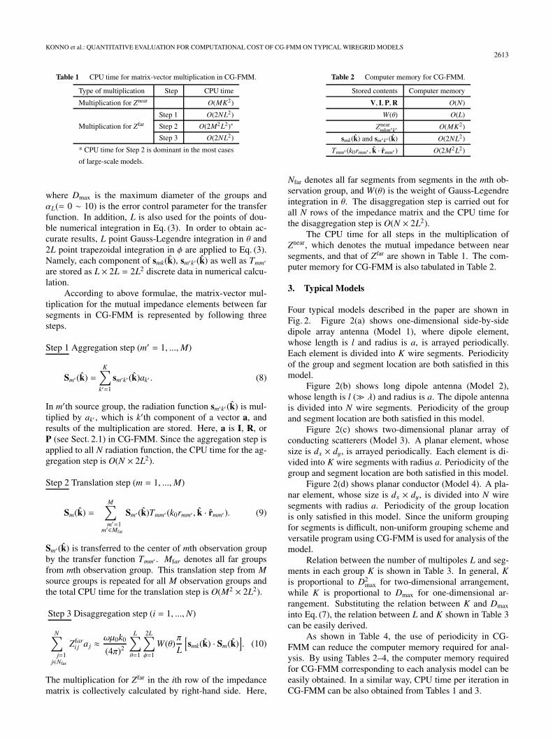
Table 1 CPU time for matrix-vector multiplication in CG-FMM.

Type of multiplication Step CPU time

Multiplication for Znear O(MK2)

Step 1 O(2NL2)

Multiplication for Zfar Step 2 O(2M2L2)∗

Step 3 O(2NL2)

* CPU time for Step 2 is dominant in the most cases

of large-scale models.

where Dmax is the maximum diameter of the groups andαL(= 0 ∼ 10) is the error control parameter for the transferfunction. In addition, L is also used for the points of dou-ble numerical integration in Eq. (3). In order to obtain ac-curate results, L point Gauss-Legendre integration in θ and2L point trapezoidal integration in φ are applied to Eq. (3).Namely, each component of smk(k), sm′k′(k) as well as Tmm′

are stored as L × 2L = 2L2 discrete data in numerical calcu-lation.

According to above formulae, the matrix-vector mul-tiplication for the mutual impedance elements between farsegments in CG-FMM is represented by following threesteps.

Step 1 Aggregation step (m′ = 1, ...,M)

Sm′(k) =K∑

k′=1

sm′k′(k)ak′ . (8)

In m′th source group, the radiation function sm′k′(k) is mul-tiplied by ak′ , which is k′th component of a vector a, andresults of the multiplication are stored. Here, a is I, R, orP (see Sect. 2.1) in CG-FMM. Since the aggregation step isapplied to all N radiation function, the CPU time for the ag-gregation step is O(N × 2L2).

Step 2 Translation step (m = 1, ...,M)

Sm(k) =M∑m′=1

m′∈Mfar

Sm′(k)Tmm′ (k0rmm′ , k · rmm′). (9)

Sm′ (k) is transferred to the center of mth observation groupby the transfer function Tmm′ . Mfar denotes all far groupsfrom mth observation group. This translation step from Msource groups is repeated for all M observation groups andthe total CPU time for the translation step is O(M2 × 2L2).

Step 3 Disaggregation step (i = 1, ...,N)

N∑j=1

j∈Nfar

Zfari j a j ≈ ωμ0k0

(4π)2

L∑θ=1

2L∑φ=1

W(θ)π

L

[smk(k) · Sm(k)

]. (10)

The multiplication for Zfar in the ith row of the impedancematrix is collectively calculated by right-hand side. Here,

Table 2 Computer memory for CG-FMM.

Stored contents Computer memory

V, I,P,R O(N)

W(θ) O(L)

Znearmkm′k′ O(MK2)

smk(k) and sm′k′ (k) O(2NL2)

Tmm′ (k0rmm′ , k · rmm′ ) O(2M2L2)

Nfar denotes all far segments from segments in the mth ob-servation group, and W(θ) is the weight of Gauss-Legendreintegration in θ. The disaggregation step is carried out forall N rows of the impedance matrix and the CPU time forthe disaggregation step is O(N × 2L2).

The CPU time for all steps in the multiplication ofZnear, which denotes the mutual impedance between nearsegments, and that of Zfar are shown in Table 1. The com-puter memory for CG-FMM is also tabulated in Table 2.

3. Typical Models

Four typical models described in the paper are shown inFig. 2. Figure 2(a) shows one-dimensional side-by-sidedipole array antenna (Model 1), where dipole element,whose length is l and radius is a, is arrayed periodically.Each element is divided into K wire segments. Periodicityof the group and segment location are both satisfied in thismodel.

Figure 2(b) shows long dipole antenna (Model 2),whose length is l (� λ) and radius is a. The dipole antennais divided into N wire segments. Periodicity of the groupand segment location are both satisfied in this model.

Figure 2(c) shows two-dimensional planar array ofconducting scatterers (Model 3). A planar element, whosesize is dx × dy, is arrayed periodically. Each element is di-vided into K wire segments with radius a. Periodicity of thegroup and segment location are both satisfied in this model.

Figure 2(d) shows planar conductor (Model 4). A pla-nar element, whose size is dx × dy, is divided into N wiresegments with radius a. Periodicity of the group locationis only satisfied in this model. Since the uniform groupingfor segments is difficult, non-uniform grouping scheme andversatile program using CG-FMM is used for analysis of themodel.

Relation between the number of multipoles L and seg-ments in each group K is shown in Table 3. In general, Kis proportional to D2

max for two-dimensional arrangement,while K is proportional to Dmax for one-dimensional ar-rangement. Substituting the relation between K and Dmax

into Eq. (7), the relation between L and K shown in Table 3can be easily derived.

As shown in Table 4, the use of periodicity in CG-FMM can reduce the computer memory required for anal-ysis. By using Tables 2–4, the computer memory requiredfor CG-FMM corresponding to each analysis model can beeasily obtained. In a similar way, CPU time per iteration inCG-FMM can be also obtained from Tables 1 and 3.

2614IEICE TRANS. COMMUN., VOL.E93–B, NO.10 OCTOBER 2010

Fig. 2 Four typical wiregrid models.

Table 3 Relation between L and K.

Segment arrangement Relation between L and K

1D (Models 1 and 2) L ∝ K

2D (Models 3 and 4) L2 ∝ K

Table 4 Computer memory reduction using periodicity in CG-FMM.

Type of periodicity Required computer memory

in analysis model

Znearmkm′k′ Tmm′ smk, sm′k′

None O(MK2) O(2M2L2) O(2NL2)

Group location O(MK2) O(2ML2) O(2NL2)

Group and segment O(K2) O(2ML2) O(2KL2)

location

4. Numerical Results

In this section, numerical analysis of four typical models iscarried out using the Richmond’s MoM [2]. Dell PrecisionPWS 380 with 2 GB RAM is used for all numerical calcu-

lation. ε = 10−4 is used for the convergence criterion ofCG-FMM and αL = 2 is employed to Eq. (7) for sufficienttruncation number. In addition, the self impedance and themutual impedance between segments in adjacent groups arecalculated by the MoM, rather than by FMM. Initial valueof current vector I is zero vector. Preconditioning techniqueis not used in both CG method and CG-FMM.

4.1 Number of Iteration Steps and Condition Number

The number of iteration steps required for CG method andCG-FMM and the condition number κ of Z for four typicalmodels are shown in Fig. 3. The condition number κ of Z isdefined by

κ =

√λmax

λmin. (11)

where λmax and λmin are the maximum and minimum eigen-value of Z†Z, respectively. As shown in Fig. 3, the tendencyof the condition number κ is almost the same to that of thenumber of iteration steps determined by error control pa-rameter. From those results, it is found that the condition

KONNO et al.: QUANTITATIVE EVALUATION FOR COMPUTATIONAL COST OF CG-FMM ON TYPICAL WIREGRID MODELS2615

Fig. 3 Number of iteration steps and condition number of Z.

number is highly related to that of the number of iterationsteps.

Large κ means that the impedance matrix Z is ill-conditioned and convergence of the solution obtained in it-erative procedure is slow. On the other hand, small κ meansthat the impedance matrix Z is well-conditioned and conver-gence of the solution is fast.

From a physical point of view, condition number κ in-dicates how the solution I in Eq. (1) is sensitive to the valuesof the elements in the impedance matrix Z. When electri-cal connection between segments in the model is strong dueto linear-connection of segments or strong mutual couplingsuch as Models 2 and 3, the condition number κ increases asshown in Figs. 3(b) and 3(c), and I is sensitive to Z. On theother hand, when electrical connection between segmentsin the model is weak due to small mutual coupling or grid-connection of segments such as Models 1 and 4, conditionnumber κ is small as shown in Figs. 3(a) and 3(d), and I isnot sensitive to Z. Constant κ shown in Figs. 3(a) and 3(c)means that mutual coupling effect to an element does notchange anymore even if M increases. In general, since cur-rent of each segment is affected by all segments, the num-

ber of iteration steps required for analysis increases whennumber of segments N increases. However, mutual cou-pling effect to I from significantly far elements is very smalland negligible in the array antenna such as Models 1 and3. Therefore, κ and number of iteration steps required foranalysis of the array antenna which has enough number ofelements becomes constant.

4.2 CPU Time per Iteration

The CPU time per iteration for analysis of four typical mod-els is shown in Fig. 4. It is found that the CPU time per it-eration of CG-FMM is O(N2) for the Models 1 and 2, whilethat for the Models 3 and 4 is reduced to O(N1.5). UsingL ∝ K shown in Table 3, it can be derived from Table 1 thatthe CPU time per iteration for analysis of one-dimensionalmodels is O(N2), which is independent of the value of M,because the CPU time of Step 2 in Table 1 is O(N2). InFig. 4(c), the order of the CPU time per iteration is O(N),when N is small. Since K is constant (= 84) in the model3, it is easy to understand that K � M when N(= MK) isas small as about 1000 or less. Based on L2 ∝ K shown in

2616IEICE TRANS. COMMUN., VOL.E93–B, NO.10 OCTOBER 2010

Fig. 4 CPU time per iteration for analysis.

Table 5 Computational cost of CG-FMM for four typical wiregrid models.

Item Model 1 Model 2 Model 3 Model 4

Properties of Segment arrangement 1D 1D 2D 2D

analysis model Segment connection Linearly connected Linearly connected Grid connected Grid connected

Number of elements Array Single Array Single

Type of periodicity Group location Used Used Used Used

used in CG-FMM Segment location Used Used Used Not used

Relation between L and K L ∝ K L ∝ K L2 ∝ K L2 ∝ K

Parameter setting on grouping K = Const. M = K =√

N K = Const. M = K =√

N

Number of iteration steps Const. O(N) O(N0.5)→ Const. O(N0.25)

Computational cost CPU time per iteration O(N2) O(N2) O(N)→ O(N1.5) O(N1.5)

Total CPU time O(N2) O(N3) O(N1.5) O(N1.75)

Computer memory O(K3)→ O(N) O(N1.5) O(K2)→ O(N) O(N1.5)

Table 3 and K(= Const.) � M, it can be obtained from Ta-ble 1 that the CPU time per iteration for analysis of model3 is O(N) when N is small. From these results, it is con-cluded that the CPU time per iteration to analyze an antennawhich has one-dimensional segment arrangement can not bereduced by CG-FMM.

4.3 Computer Memory

The order of the computer memory required for analysis ofeach model can be theoretically derived from Tables 2–4without running programs and is tabulated in Table 5. From

KONNO et al.: QUANTITATIVE EVALUATION FOR COMPUTATIONAL COST OF CG-FMM ON TYPICAL WIREGRID MODELS2617

the Table 5, it is found that the computer memory requiredfor analysis of any models is smaller than O(N2) in CG-FMM. For the array antenna/scatterer such as the Models 1and 3, the computer memory for smk and sm′k′ is dominant forthe total computer memory when M is very small. On theother hand, the computer memory for Tmm′ is dominant forthe total computer memory when M is larger than K. There-fore, the order of the computer memory required for analysisvaries as O(K3) → O(N) for Model 1 and O(K2) → O(N)for Model 3.

The order of the number of iteration steps, CPU timeper iteration, total CPU time and computer memory is tabu-lated in Table 5.

5. Conclusion

In this paper, relation between the computational cost ofCG-FMM and the analysis model was quantitatively evalu-ated by numerical simulation for four typical wire antennasor wiregrid models. It is found that the number of iterationsteps required for analysis by CG-FMM depends on the con-dition number of Z. From discussion of relation between thecondition number κ and electrical properties of the models,it is shown that the condition number κ becomes large dueto linear-connection of segments or strong mutual couplingbetween elements. Similarly, it is shown that the condi-tion number κ becomes small due to grid-connection of seg-ments exist or weak mutual coupling between elements. Thecomputer memory required for analysis are reduced fromO(N2) for all models by the use of CG-FMM. On the otherhand, it is shown that the CPU time per iteration can be re-duced only for models which has two-dimensional segmentarrangement in each group.

Since the models for analysis used in this paper aresimple linear or planar models, the computational cost ofCG-FMM for more complicated structures is desired to beevaluated. In addition, the computational cost of CG-FMMapplied to the Rao-Wilton-Glisson (RWG) basis function[24] as well as the Schaubert-Wilton-Glisson (SWG) ba-sis function [25] is expected to be evaluated for analysis ofstructures including dielectric bodies.

Acknowledgments

This work was supported by the GCOE Program CERIESin Tohoku University, and SCAT (Support Center for Ad-vanced Telecommunications) Technology Research, Foun-dation. Supercomputing resources at Cyberscience Centerin Tohoku University were used in process of this research.

References

[1] R.F. Harrington, Field Computation by Moment Methods, Macmil-lan, New York, 1968.

[2] J.H. Richmond and N.H. Greay, “Mutual impedance of nonplanar-skew sinusoidal dipoles,” IEEE Trans. Antennas Propag., vol.AP-23,no.5, pp.412–414, May 1975.

[3] T.K. Sarkar and S.M. Rao, “The application of the conjugate gradi-ent method for the solution of electromagnetic scattering from ar-bitrarily oriented wire antennas,” IEEE Trans. Antennas Propag.,vol.AP-32, no.4, pp.398–403, April 1984.

[4] T.K. Sarkar, “The conjugate gradient method as applied to elec-tromagnetic field problems,” IEEE Antennas Propagation SocietyNewsletter, vol.28, no.4, pp.4–14, Aug. 1986.

[5] J. Tang, “Numerical aspects of iterative solving of linear systemsderived from Helmholtz’s problem,” Literature Report of Delft Uni-versity of Technology, Feb. 2004.

[6] T.K. Sarkar, K.R. Siarkiewicz, and S.M. Rao, “Survey of numericalmethods for solution of large systems of linear equations for electro-magnetic field problems,” IEEE Trans. Antennas Propag., vol.AP-29, no.6, pp.847–856, Nov. 1981.

[7] A.F. Peterson and R. Mittra, “Convergence of the conjugate gradientmethod when applied to matrix equations representing electromag-netic scattering problems,” IEEE Trans. Antennas Propag., vol.AP-34, no.12, pp.1447–1454, Dec. 1986.

[8] A.F. Peterson, C.F. Smith, and R. Mittra, “Eigenvalues of themoment-method matrix and their effect on the convergence ofthe conjugate gradient algorithm,” IEEE Trans. Antennas Propag.,vol.36, no.8, pp.1177–1179, Aug. 1988.

[9] R. Coifuman, V. Rokhlin, and S. Wandzura, “The fast multipolemethod for the wave equation: A pedestrian prescription,” IEEE An-tennas Propag. Mag., vol.35, no.3, pp.7–12, June 1993.

[10] V. Rokhlin, “Rapid solution of integral equations of scattering theoryin two dimension,” J. Comput. Phys., vol.86, no.2, pp.414–439, Feb.1990.

[11] J.M. Song and W.C. Chew, “Multilevel fast-multipole algorithm forsolving combined field integral equations of electromagnetic scat-tering,” Microw. Opt. Technol. Lett., vol.10, no.1, pp.14–19, Sept.1995.

[12] J.M. Song, C.C. Lu, and W.C. Chew, “Multilevel fast multipole al-gorithm for electromagnetic scattering by large complex objects,”IEEE Trans. Antennas Propag., vol.45, no.10, pp.1488–1493, Oct.1997.

[13] I. Bogaert, J. Peeters, and F. Olyslager, “A nondirective plane waveMLFMA stable at low frequencies,” IEEE Trans. Antennas Propag.,vol.56, no.12, pp.3752–3767, Dec. 2008.

[14] J. Fostier and F. Olyslager, “An asynchronous parallel MLFMAfor scattering at multiple dielectric objects,” IEEE Trans. AntennasPropag., vol.56, no.8, pp.2346–2355, Aug. 2008.

[15] O. Ergul and L. Gurel, “Efficient parallelization of the multilevel fastmultipole algorithm for the solution of large-scale scattering prob-lems,” IEEE Trans. Antennas Propag., vol.56, no.8, pp.2335–2345,Aug. 2008.

[16] O. Ergul and L. Gurel, “Comparison of integral-equation formula-tions for the fast and accurate solution of scattering problems involv-ing dielectric objects with the multilevel fast multipole algorithm,”IEEE Trans. Antennas Propag., vol.57, no.1, pp.176–187, Jan. 2009.

[17] A. Tzoulis and T.F. Eibert, “Efficient electromagnetic near-fieldcomputation by the multilevel fast multipole method employingmixed near-field/far-field translations,” IEEE Antennas WirelessPropag. Lett., vol.4, pp.449–452, 2005.

[18] Ismatullah and T.F. Eibert, “Surface integral equation solutions byhierarchical vector basis functions and spherical harmonics basedmultilevel fast multipole method,” IEEE Trans. Antennas Propag.,vol.1, no.1, pp.1–14, Jan. 2010.

[19] I. Hanninen and J. Sarvas, “Efficient evaluation of the Rohklin trans-lator in multilevel fast multipole algorithm,” IEEE Trans. AntennasPropag., vol.56, no.8, pp.2356–2362, Aug. 2008.

[20] T. Dufva and J. Sarvas, “Broadband MLFMA with plane waveexpansions and optimal memory demand,” IEEE Trans. AntennasPropag., vol.57, no.3, pp.742–753, March 2009.

[21] S.S. Bindiganavale and J.L. Volakis, “Guidelines for using the fastmultipole method to calculate the RCS of large objects,” Microw.Opt. Technol. Lett., vol.11, no.4, pp.190–194, March 1996.

2618IEICE TRANS. COMMUN., VOL.E93–B, NO.10 OCTOBER 2010

[22] Z. Yaojiang, G. Zhonglin, Z. Lezhu, and F. Zhenghe, “Guide-lines of parameter settings in 3D fast multipole method,” Proc.ICMMT2000, pp.387–390, Beijing, China, Sept. 2000.

[23] M. Abramowitz and I.A. Stegum, Handbook of Mathematical Func-tions, National Bureau of Standards, 1972.

[24] S.M. Rao, D.R. Wilton, and A.W. Glisson, “Electromagnetic scatter-ing by surfaces of arbitrary shape,” IEEE Trans. Antennas Propag.,vol.AP-30, no.3, pp.409–418, May 1982.

[25] D.H. Schaubert, D.R. Wilton, and A.W. Glisson, “A tetrahedral mod-eling method for electromagnetic scattering by arbitrarily shapedinhomogeneous dielectric bodies,” IEEE Trans. Antennas Propag.,vol.AP-32, no.1, pp.77–85, Jan. 1984.

Keisuke Konno received the B.E. and M.E.degrees from Tohoku University, Sendai, Japan,in 2007 and 2009, respectively. Currently, heworks for the D.E. degree at the Department ofElectrical Communication Engineering in Grad-uate School of Engineering, Tohoku Univer-sity. His research interests include computa-tional electromagnetics, array antennas.

Qiang Chen received the B.E. degree fromXidian University, Xi’an, China, in 1986, theM.E. and D.E. degrees from Tohoku University,Sendai, Japan, in 1991 and 1994, respectively.He is currently an Associate Professor with theDepartment of Electrical Communications, To-hoku University. His primary research interestsinclude computational electromagnetics, arrayantennas, and antenna measurement. Dr. Chenreceived the Young Scientists Award in 1993,the Best Paper Award in 2008 from the Insti-

tute of Electronics, Information and Communication Engineers (IEICE) ofJapan. Dr. Chen is a member of the IEEE. He has served as the Secretaryand Treasurer of IEEE Antennas and Propagation Society Japan Chapter in1998, the Secretary of Technical Committee on Electromagnetic Compat-ibility of IEICE from 2004 to 2006. He is now the Secretary of TechnicalCommittee on Antennas and Propagation of IEICE, Associate Editor ofIEICE Transactions on Communications.

Kunio Sawaya received the B.E., M.E.and D.E. degrees from Tohoku University, Sen-dai, Japan, in 1971, 1973 and 1976, respectively.He is presently a Professor in the Departmentof Electrical and Communication Engineeringat the Tohoku University. His areas of inter-ests are antennas in plasma, antennas for mo-bile communications, theory of scattering anddiffraction, antennas for plasma heating, and ar-ray antennas. He received the Young ScientistsAward in 1981, the Paper Award in 1988, Com-

munications Society Excellent Paper Award in 2006, and Zen-ichi KiyasuAward in 2009 all from the Institute of Electronics, Information and Com-munication Engineers (IEICE). He served as the Chairperson of the Tech-nical Group of Antennas and Propagation of IEICE from 2001 to 2003,the Chairperson of the Organizing and Steering Committees of 2004 In-ternational Symposium on Antennas and Propagation (ISAP’04) and thePresident of the Communications Society of IEICE from 2009 to 2010.Dr. Sawaya is a senior member of the IEEE, and a member of the Instituteof Image Information and Television Engineers of Japan.