Paper or Plastic?

Money and Credit as Means of Payment∗

Sebastien Lotz†

LEMMA, University of Paris 2Cathy Zhang‡

University of California-Irvine

April 19, 2013

Abstract

This paper studies the choice of payment instruments in a simple model where both moneyand credit can be used as means of payment. We endogenize the acceptability of credit byallowing retailers to invest in a costly record-keeping technology. Our framework captures thetwo-sided market interaction between consumers and retailers, leading to strategic complemen-tarities that can generate multiple steady-state equilibria. In addition, limited commitmentmakes debt contracts self-enforcing and yields an endogenous upper bound on credit use. Ourmodel can explain why the demand for credit declines as inflation falls, and how hold-up prob-lems in technological adoption can prevent retailers from accepting credit as consumers continueto coordinate on cash usage. We show that whenever money and credit coexist, equilibrium isgenerically inefficient and optimal policy entails an inflation rate strictly above the Friedmanrule. We also discuss the extent to which our model can reconcile some key patterns in the useof cash and credit in retail transactions.

Keywords: coexistence of money and credit, inflation, costly record-keeping, credit constraintsJEL Classification Codes: D82, D83, E40, E50

∗We are indebted to Guillaume Rocheteau for extremely valuable discussions and feedback throughout this project.We also thank Pedro Gomis-Porqueras and Janet Jiang for providing many useful comments and suggestions.†Address: LEMMA, Universite Pantheon-Assas-Paris II, 92 rue d’Assas, 75006 Paris, France. E-mail: lotz@u-

paris2.fr.‡Address: Department of Economics, University of California at Irvine, 3151 Social Science Plaza, Irvine, CA

92697-5100, USA. E-mail: cmzhang@uci.edu.

1 Introduction

Consumers now have more payment instruments than ever to choose from, ranging from cash, credit

cards, prepaid cards, smart cards, mobile account payments, and electronic money (“e-money”).1

According to Gerdes, Walton, Liu, and Parke (2005), innovations in the retail landscape have

generated a payments transformation, as card payments now dominate more traditional paper-

based ones.2 In particular, technological improvements in electronic record-keeping have made

credit cards as ubiquitous as cash as means of payment in many OECD countries. A recent study

by the Federal Reserve finds that the number of payments made by general-purpose credit cards

rose from 15.2 billion to 19.0 billion between 2003 and 2006 in the United States, for a growth rate of

7.6% a year. During this same period, the number of ATM cash withdrawals dropped slightly from

5.9 billion to 5.8 billion (Gerdes (2008)). This suggests that while consumers are indeed adopting

new payment instruments, they are not completely abandoning older ones (Schuh (2012)).

As consumers change the way they pay and businesses change the way they accept payments, it

is increasingly important to understand how consumer demand affects merchant behavior and vice

versa. In fact, the payment system is a classic example of a two-sided market where both consumers

and firms must make choices that affect one other. This dynamic often generates complementarities

and network externalities, which is a key characteristic of the retail payment market (Rysman

(2009), BIS (2012)).3 Moreover, the recent trends in retail payments raise many interesting and

challenging questions for central banks and policymakers. In particular, how does the availability

of alternative means of payment, such as credit cards, affect the role of money? And if both money

and credit can be used, how does policy and inflation affect the money-credit margin?

We investigate the possible substitution away from cash to electronic payments such as credit

cards using a simple model where money and credit can coexist as means of payment. Our objective

is to determine the impact that retail payment innovations can have on future cash usage. Under-

standing how people substitute between cash and credit is a key policy concern for central banks

when setting an inflation target, as well as legislators when developing new regulation on credit

card fees. As it is the sole issuer of bank notes, central banks also need to understand substitution

patterns to predict consumers’ demand for cash.

1Evidence from Foster, Meijer, Schuh, and Zabek (2009) reveals that in 2009, the average U.S. consumer holds5.0 of the nine most common payment instruments and used 3.8 of them during a typical month.

248.8% of transactions recorded in the Federal Reserve Bank of Boston’s 2010 Survey of Consumer Payment Choicewere conducted with payment cards, while 40.8% of transactions used paper instruments, such as cash or check.

3Network externalities exist when the value of a good or service to a potential user increases with the number ofother users using the same product. Credit cards are a good example of network good, where its adoption and usecan be below the socially optimal level because consumers or firms do not internalize the benefit of their own use onothers’ use. For evidence and a discussion of the empirical issues, see Gowrisankaran and Stavins (2004).

1

To capture the two-sided nature of actual payment systems, our model focuses on the market

interaction between consumers (buyers, or borrowers) and retailers (sellers, or lenders). A vital

distinction between monetary and credit trades is that the former is quid pro quo and settled on

the spot while the latter involves delayed settlement.4 For credit to have a role, we introduce a costly

record-keeping technology that allows transactions to be recorded.5 A retailer that invests in this

technology will thus be able to accept an IOU from a consumer. In this way, credit allow retailers

to sell to illiquid consumers or to those paying with future income. Due to limited commitment

and enforcement however, lenders cannot force borrowers to repay their debts. In order to motivate

voluntary debt repayment, we assume that default by the borrower triggers a global punishment

that banishes agents from all future credit transactions. In that case, a defaulter can only trade

with money. Consequently, debt contracts must be self-enforcing and the possibility of strategic

default generates an endogenous upper-bound on credit use.6

When enforcement is imperfect, inflation has two effects: a higher inflation rate both lowers

the rate of return on money and makes default more costly. This relaxes the credit constraint and

induces agents to shift from money to credit to finance their consumption. Consequently, consumers

decrease their borrowing as inflation falls. When lump-sum taxes can be enforced and the monetary

authority implements the Friedman rule, deflation completely crowds out credit and there is a flight

to liquidity where all borrowing and lending ceases to exist. In that case, efficient monetary policy

drives out credit.7 However when both money and credit are used, the Friedman rule is not feasible

to sustain voluntary debt repayment. When borrowers are not patient enough, inflation has a

hump-shaped effect on welfare and optimal policy entails a strictly positive inflation rate. While

equilibrium is typically inefficient when money and credit coexist, the first-best allocation can still

be achieved in a pure credit economy, provided that agents are patient enough. However equilibrium

is not socially efficient since sellers must incur the real cost of technological adoption.

4This distinction separates debit cards, which are “pay now” cards, from credit cards, or “pay later” cards. Fordebit cards, funds are typically debited from the cardholder’s account within a day or two of purchase, while creditcards allow consumers to access credit lines at their bank which are repaid at a future date. In this paper, we interpretcredit trades as occurring with credit cards and monetary trades as those occurring with cash or debit.

5As is well established by now, the same frictions that render money essential make credit arrangements impossible.These frictions include imperfect record-keeping over individual trading histories, lack of commitment, and lack ofenforcement. See e.g. Kocherlakota and Wallace (1998).

6This is in the spirit of Kehoe and Levine (1993) and Alverez and Jermann (2000) where the threat of banishmentfrom future credit transactions motivate voluntary debt repayment.

7In our model, the presence of multiple steady-state equilibria where either money, credit, or both are used makesthe choice of optimal policy difficult to analyze in full generality. If the monetary authority must choose an inflationrate before it knows which equilibrium will obtain, policy will affect the equilibrium selection process. Instead ofspecifying equilibrium selection rules, we suppose the existence of a particular equilibrium and then analyze theoptimal policy in that equilibrium. In models where the fraction of credit trades is fixed, limited commitment andimperfect enforcement can also lead to a positive optimal inflation rate; see e.g. Berentsen, Camera, and Waller(2007), Antinolfi, Azariadis, and Bullard (2009), and Gomis-Porqueras and Sanches (2011).

2

The channel through which monetary policy affects macroeconomic outcomes is through buyers’

choice of portfolio holdings, sellers’ decision to invest in the record-keeping technology, and the

endogenously determined credit constraint. If sellers must invest ex-ante in a costly technology

to record credit transactions, there are strategic complementarities between the seller’s decision to

invest and the buyer’s ability to repay. When more sellers accept credit, the gain for buyers from

using and redeeming credit increases, which relaxes the credit constraint. At the same time, an

increase in the buyer’s ability to repay raises the incentive to invest in the record-keeping technology

and hence the fraction of credit trades. This complementarity leads to feedback effects that can

generate multiple steady-state equilibria, including outcomes where both money and credit are

used.8

Moreover, this channel mimics the mechanism behind two-sided markets in actual payment

systems as described by McAndrews and Zhu (2008): merchants are more willing to accept credit

cards that have many cardholders, and cardholders want cards that are accepted at many estab-

lishments. Just as in our model, the payment network benefits the merchant and the consumer

jointly, leading to the same kind of complementarities and network externalities highlighted in the

industrial organization literature. At the same time, consumers may still coordinate on using cash

due to a hold-up problem in technological adoption. Since retailers do not receive the full surplus

associated with technological adoption, they fail to internalize the total benefit of accepting credit.

The choice of payment instruments will therefore depend on fundamentals, as well as history and

social conventions.

This potential for coordination failures also raises new concerns for policymakers. In contrast

with conventional wisdom, our theory suggests that economies with similar technologies, institu-

tions, and policies can still end up with very different payment systems, some being better in terms

of social welfare than others. If for example society prefers a payment system with only credit, the

government may want to introduce special policies such as information campaigns, advertisements,

or even financial literacy programs that help coordinate agents on using credit. These measures

that enhance communication are especially relevant for many emerging economies where the lack of

financial infrastructure and intermediation makes new forms of mobile credit payments particularly

appealing.9 Hence our model not only provides policymakers a useful framework for understanding

how consumers substitute between money and credit, but also makes clear the channels through

which their policies affect prices, trade, and social welfare.

8This multiplicity is consistent with empirical evidence from Humphreys, Pulley, and Vesala (1996) that findsinertia in the adoption of new payment instruments.

9For example, the November 17, 2012 Economist article “War of the Virtual Wallets” predicts that “the biggestprize of all lies in emerging markets where a lack of financial infrastructure is hastening the rise of phone-basedpayments systems.”

3

The remainder of the paper proceeds as follows. Section 1.1 reviews the related literature.

Section 2 describes the basic environment with limited enforcement. Section 3 then determines

equilibrium where an exogenous fraction of sellers accept credit. Section 4 determines the endoge-

nous debt limit and characterizes properties of monetary and non-monetary equilibrium with credit.

Section 5 endogenizes the fraction of credit trades and discusses multiplicity. Section 6 turns to

normative considerations and discusses welfare and optimal monetary policy, and Section 7 relates

our model with the empirical evidence on consumer payments. Finally, Section 8 concludes.

1.1 Related Literature

Within modern monetary theory, there is a strong tradition of studying the coexistence of money

and credit. Shi (1996) provides the first model with bargaining, money, and credit and shows that

money can coexist with credit that yields a higher rate of return. In Kocherlakota and Wallace

(1998), an equilibrium with money and credit can be sustained if individual histories are made

public with a lag.10 In another approach, Berentsen, Camera, and Waller (2007) models credit as

bank loans in an environment with limited enforcement. However money remains the only means of

payment since goods transactions remain private information for banks.11 Sanches and Williamson

(2010) get money and credit to coexist in a divisible money model with imperfect memory, limited

commitment, and theft, while Bethune, Rocheteau, and Rupert (2013) develop a model with credit

and liquid assets to examine the relationship between unsecured debt and unemployment. Gu and

Wright (2012) use a related framework to study dynamics in a pure credit economy. However in

all these approaches, only an exogenous subset of agents can use credit while the choice of using

credit is endogenous in this paper.12

Our model of costly record-keeping is based on the model of money and costly credit in Nosal

and Rocheteau (2010), though a key novelty is that we derive an endogenous debt limit under

limited commitment instead of assuming that loan repayments can be perfectly enforced. Dong

(2011) also introduces costly record-keeping, but focuses on the buyer’s choice of payments used in

bilateral meetings.13 Our paper is the first to model the two-sided nature of accepting payments

in an environment where money and credit can coexist and enforcement is limited.

Closely related to our paper is Gomis-Porqueras and Sanches (2011), who also discuss the role of

10A related approach assumes limited participation to allow for monetary and credit transactions; see e.g. Calva-canti and Wallace (1999), Williamson (1999), Williamson (2004), and Mills (2007), among many others.

11See also Telyukova and Wright (2008) for a model with divisible money and IOUs issued in a competitive market.12In a similar vein, Schreft (1992) and Dotsey and Ireland (1996) introduce costs paid to financial intermediaries

to endogenize the composition of trades that use money or credit, and Prescott (1987) and Freeman and Kydland(2000) feature a fixed record-keeping cost for transactions made with demand deposits.

13Arango and Taylor (2008) and Turban (2008) find that record-keeping or other technological costs associatedwith accepting credit are incurred by the seller.

4

money and credit in a model with anonymity, limited commitment, and imperfect record-keeping.

A key difference in the set-up is that they adopt a different pricing mechanism by assuming a

buyer-take-all bargaining solution. While this assumption may seem innocuous, our assumption of

proportional bargaining allows us to take the analysis further in two important ways.14 By giving

the seller some bargaining power, proportional bargaining allows us to endogenize the fraction of

sellers that can accept credit by allowing them to invest in a costly record-keeping technology. This

also allows us to discuss hold-up problems on the seller’s side which will lead to complementarities

with the buyer’s borrowing limit. This generates interesting multiplicities and network effects that

the previous study cannot discuss.

This paper is also related to a growing strand in the industrial organization literature that

examines the costs and benefits of credit cards to network participants. In particular, recent

work by Wright (2003) and Rochet and Tirole (2011) models the bilateral transactions between

consumers and retailers to study the effects of regulatory policies and market structure in the credit

card industry.15 However, this literature abstracts from a critical distinction between monetary and

credit transactions by ignoring the actual borrowing component of credit transactions.

By contrast, our paper is explicit about the intertemporal nature of credit transactions by

allowing consumers to issue an IOU to the seller, or paying on the spot with cash. In turn, our

framework can be used to determine the conditions under which consumers prefer one type of

payment instrument over the other, and how this can be affected by policy. As new forms of

payment develop and become increasingly prevalent, these issues are central concerns that both

central banks and policymakers need to understand.

2 Environment

The economy consists of a continuum [0, 2] of infinitely lived agents, evenly divided between buyers

(or consumers) and sellers (or retailers). Time is discrete and continues forever. Each period is

divided into two sub-periods where economic activity will differ. In the first sub-period, agents meet

pairwise and at random in a decentralized market, called the DM . Sellers can produce output,

q ∈ R+, but do not want to consume, while buyers want to consume but cannot produce. Agents’

identities as buyers or sellers are permanent, exogenous, and determined at the beginning of the

14More generally, proportional bargaining guarantees that trade is pairwise Pareto efficient and has several desirablefeatures that cannot be guaranteed with Nash bargaining, as discussed in Aruoba, Rocheteau, and Waller (2007).First, it guarantees the concavity of agent’s value functions. Second, the proportional solution is monotonic and hencedoes not suffer from a shortcoming of Nash bargaining that an agent can end up with a lower individual surplus evenif the size of the total surplus increases.

15Chakravorti (2003) provides a theoretical survey of the industrial organization approach to credit card networks,and Rysman (2009) gives an overview of the economics of two-sided markets.

5

DM. In the second sub-period, trade occurs in a frictionless centralized market, called the CM ,

where all agents can consume a numeraire good, x ∈ R+, by supplying labor, y, one-for-one using

a linear technology.

Instantaneous utility functions of buyers, (U b), and sellers, (U s), are assumed to be separable

between sub-periods and linear in the CM:

U b (q, x, y) = u (q) + x− y,

U s (q, x, y) = −c (q) + x− y.

Functional forms for utility and cost functions in the DM, u(q) and c(q) respectively, are assumed

to be C2 with u′ > 0, u′′ < 0, c′ > 0, c′′ > 0, u(0) = c(0) = c′(0) = 0, and u′(0) = ∞. Also, let

q∗ ≡ q : u′(q∗) = c′(q∗). All agents discount the future between periods, but not sub-periods,

with a discount factor β ∈ (0, 1).

The only asset in this economy is fiat money, which is perfectly divisible and storable. Money

m ∈ R+ is valued at φ, the price of money in terms of numeraire. Its aggregate stock in the

economy, M , can grow or shrink each period at a constant gross rate γ ≡ Mt+1

Mt. Changes in the

money supply are facilitated through lump-sum transfer or taxes in the CM to buyers. In the

latter case, we assume that the government has sufficient enforcement so that agents will repay the

lump-sum tax.16

To purchase goods in the DM, both monetary and credit transactions are feasible due to the

availability of a record-keeping technology that can record agent’s transactions. However this

technology is only available to a fraction Λ ∈ [0, 1] of sellers, while the remaining 1− Λ sellers can

only accept money. For example, the cost function is such that investment in this technology is

infinitely costly for a fraction 1−Λ of firms while costless for the remaining Λ firms. In Section 5,

we endogenize Λ by considering an alternative cost function where sellers have heterogenous costs

of investing.

We assume that contracts written in the DM can be repaid in the subsequent CM. Buyers can

issue b ∈ R+ units of one-period IOUs that we normalize to be worth one unit of the numeraire good.

While the record-keeping technology can identify agents and record their transactions, enforcement

may be imperfect. This leads to the possibility of strategic default by the borrower. In order to

16While the government can never observe agents’ real balances, it has the authority to impose arbitrarily harshpenalties on agents who do not pay taxes when γ < 1. Alternatively, Andolfatto (2007) considers an environmentwhere the government’s enforcement power is limited and the payment of lump-sum taxes is voluntary. This inducesa lower bound on the deflation rate in which case the Friedman rule fails to be incentive feasible even though itis desirable. Alternatively, if the monetary authority does not want to implement deflation, it can still achieve thefirst-best allocation by paying interest on currency financed by increases in the money supply, as discussed in GomisPorqueras and Peralta-Alva (2010) and Nosal and Rocheteau (2011).

6

Figure 1: Timing of Representative Period

support trade in a credit economy, potential borrowers must be punished if they do not deliver

on their promise to repay. We assume that punishment for default entails permanent exclusion

from the credit system.17 In that case, a borrower who defaults can only use money for all future

transactions.

The timing of events in a typical period is summarized in Figure 1. At the beginning of the

DM, a measure σ of buyers and sellers are randomly matched, where the buyer has m ∈ R+ units

of money, or equivalently, z = φm units of real balances. Terms of trade are determined using a

proportional bargaining rule. In the CM, buyers produce the numeraire good, redeem their loan,

and acquire money, while sellers can purchase the numeraire with money and can get their loan

repaid. We focus on stationary equilibria where real balances are constant over time.

3 Equilibrium

The model can be solved in four steps. First, we characterize properties of agents’ value functions

in the CM. Using these properties, we then determine the terms of trade in the DM. Third, we

determine the buyer’s choice of asset holdings, and in Section 4 we characterize equilibrium with

the endogenous debt limit. Then in Section 5, we determine Λ endogenously by allowing sellers to

17Starting with Kehoe and Levine (1993) and Alverez and Jermann (2000), off-equilibrium path punishments arealso considered by Aiyagari and Williamson (2000), Antinolfi, Azariadis, and Bullard (2007), Berentsen, Camera,and Waller (2007), Camera and Li (2008), Sanches and Williamson (2010), Gomis-Porqueras and Sanches (2011),Venkateswaran and Wright (2012), and Bethune, Rocheteau, and Rupert (2013), among many others.

7

invest in the costly record-keeping technology.

3.1 Centralized Market

In the beginning of the CM, agents consume the numeraire x, supply labor y, and readjust their

portfolios. Let W b (z,−b) denote the value function of a buyer who holds z = φm units of real

balances and has issued b units of IOUs in the previous DM. The buyer’s maximization problem at

the beginning of the CM, W b (z,−b), is

W b (z,−b) = maxx,y,z′≥0

x− y + βV b

(z′)

(1)

s.t. x+ b+ φm′ = y + z + T (2)

z′ = φ′m′ (3)

where V b is the buyer’s continuation value in the next DM and T ≡ (γ − 1)φM is the lump-sum

transfer from the government (in units of numeraire). According to (2), the buyer finances his

net consumption of numeraire (x− y), the repayment of his IOUs (b), and his following period

real balances (γz′) with his current real balances (z) and the lump-sum transfer (T ). Substituting

m′ = z′/φ′ from (3) into (2), and then substituting x− y from (2) into (1) yields

W b (z,−b) = z − b+ T + maxz′≥0

−γz′ + βV b

(z′). (4)

The buyer’s lifetime utility in the CM is the sum of his real balances net of any IOUs to be repaid,

the lump-sum transfer from the government, and his continuation value at the beginning of the next

DM net of the investment in real balances. The gross rate of return of money is φt+1

φt= Mt

Mt+1= γ−1.

Hence in order to hold z′ units of real balances in the following period, the buyer must acquire γz′

units of real balances in the current period.

Notice that W b(z,−b) is linear in the buyer’s current portfolio: W b (z,−b) = z−b+W b (0, 0). In

addition, the choice of real balances next period is independent of current real balances. Identically,

the value function W s (z, b) of a seller who holds z units of real balances and b units of IOUs can

be written:

W s (z, b) = z + b+ βV s(0)

where V s(0) is the value function of a seller at the beginning of the following DM since they have

no incentive to accumulate real balances in the DM.

8

3.2 Terms of Trade

We now turn to the terms of trade in the DM. Agents meet bilaterally, and bargain over the units

of money or IOUs to be exchanged for goods. We adopt Kalai (1977)’s proportional bargaining

solution where the buyer receives a constant share θ ∈ (0, 1) of the match surplus, while the seller

gets the remaining share, (1− θ) > 0.18

We will show that the terms of trade depend only on buyers’ portfolios and what sellers accept.

First consider a match where the seller accepts credit. In that case, the buyer holding z units of real

balances proposes a contract (q, b, d) that maximizes his expected surplus such that the seller gets

a constant share 1−θ of the total surplus. To apply the pricing mechanism, notice that the surplus

of a buyer who gets q for payment d+ b to the seller is u(q) +W b(z−d− b)−W b(z) = u(q)− b−d,

by the linearity of W b. Similarly, the surplus of a seller is −c(q) + d+ b. The bargaining problem

then becomes

(q, d, b) = arg maxq,d,bu (q)− d− b (5)

s.t. − c (q) + d+ b =1− θθ

[u (q)− d− b] (6)

d ≤ z (7)

b ≤ b. (8)

According to (5)− (8), the buyer’s offer maximizes his trade surplus such that (i) the seller’s payoff

cannot be less than a constant share 1−θθ of the buyer’s payoff, (ii) the buyer cannot transfer more

money than he has, and (iii) the buyer cannot borrow more than he can repay. Condition (7)

is a feasibility constraint on the amount the buyer can transfer to the seller, while condition (8)

is the buyer’s incentive constraint that motivates voluntary debt repayment. The threshold b is

an equilibrium object and represents the endogenous borrowing limit faced by the buyer, which is

taken as given in the bargaining problem but is determined endogenously in the next section.

Combining the feasibility constraint (7) and the buyer’s incentive constraint (8) then results in

the payment constraint

d+ b ≤ z + b (9)

which says the total payment to the seller, d+b, cannot exceed what the buyer holds, which is z+b

when the seller accepts credit. The solution to the bargaining problem will depend on whether the

payment constraint, (9), binds. If (9) does not bind, then the buyer will have sufficient wealth to

18There are also strategic foundations for the proportional bargaining solution. In Dutta (2012), Kalai (1977)’ssolution emerges as a unique equilibrium outcome in a limiting case of a Nash demand game.

9

purchase the first-best level of output, q∗. In that case, payment to the seller will be exactly

d+ b = (1− θ)u(q∗) + θc(q∗).

If (9) binds, then the buyer simply hands over what he has,

z + b = (1− θ)u(qc) + θc(qc) (10)

and gets in return qc ≡ q(z + b). Hence a buyer who does not have enough payment capacity will

just pay with their cash on hand and borrow up to their limit in order to purchase the maximum

quantity of output, qc < q∗.

If the seller does not have access to record-keeping, credit cannot be used. In that case, b = b = 0

and the bargaining problem can be described by (5)− (7). If z ≥ z∗ ≡ (1− θ)u(q∗) + θc(q∗), then

the buyer has enough payment capacity to obtain q∗. Otherwise, the buyer just hands over his real

balances,

z = (1− θ)u(q) + θc(q) (11)

where q ≡ q(z) < q∗.

3.3 Decentralized Market

We next characterize agents’ value functions the DM. After simplification, the expected discounted

utility of a buyer holding z units of real balances at the beginning of the period is:

V b (z) = σ (1− Λ) θ[u(q)− c (q)] + σΛθ [u (qc)− c (qc)] + z +W b (0, 0) , (12)

where we have used the bargaining solution and the fact that the buyer will never accumulate

more balances than he would spend in the DM. According to (12), a buyer in the DM is randomly

matched with a seller who does not have access to record-keeping with probability σ(1−Λ), receives

θ of the match surplus, u(q) − c(q), and can only pay with money. With probability σΛ, a buyer

matches with a seller with access to record-keeping, in which case he gets θ of u(qc) − c(qc) and

can pay with both money and credit. The last two terms result from the linearity of W b and is the

value of proceeding to the CM with one’s portfolio intact.

3.4 Optimal Portfolio Choice

Next, we determine the buyer’s choice of real balances. Given the linearity of W b, the buyer’s

bargaining problem (5)− (7), and substituting V b (z) from (12) into (4), the buyer’s choice of real

10

balances must satisfy:

maxz>0−iz + σ (1− Λ) θ[u(q)− c(q)] + σΛθ[u(qc)− c(qc)] (13)

where i = γ−ββ is the cost of holding real balances. As a result, the buyer chooses his real balances

z in order to maximize his expected surplus in the DM , net of the cost of holding real balances, i.

Since the objective function (13) is continuous and maximizes over a compact set, a solution

exists. We further assume u(q∗) − z(q∗) > 0 in order to guarantee the existence of a monetary

equilibrium. In the Appendix, we show that (13) is concave. The first-order condition for problem

(13) when z ≥ 0 is

− i+ σ(1− Λ)θ[u′(q)− c′(q)]

θc′(q) + (1− θ)u′(q)+ σΛ

θ[u′(qc)− c′(qc)]θc′(qc) + (1− θ)u′(qc)

≤ 0, (14)

and with equality if z > 0.

We first make a few remarks on equilibrium when enforcement is perfect. With full enforcement,

buyers are never constrained by b ≤ b and can borrow as much as they want to finance consumption

in the first-best, q∗. When z > 0, the second term on the right-hand-side of (14) equals to zero

since at q∗, u′(q∗) = c′(q∗). In that case, the right-hand-side is increasing with Λ, meaning that an

increase in the fraction of credit trades Λ decreases q(z) and hence real balances z.

4 Limited Enforcement and Credit Limits

When the government’s ability to force repayment is limited, borrowers have an incentive to renege

on their debts. In order to support trade in a credit economy, we assume that punishment for

default entails permanent exclusion from the credit system. In that case, debt-contracts must be

self-enforcing, and a borrower that defaults can no longer use credit and can only use money for

all future transactions.

The borrowing limit, b, is determined in order to satisfy the buyer’s incentive constraint to

voluntarily repay his debt in the CM:

W b (z,−b) > W b (z) ,

where W b(z,−b) is the value function of a buyer who repays his debt at the beginning of the CM,

and W b(z) is the value function of a buyer who defaults. By the linearity of W b, the value function

11

of a buyer who repays his debt in the CM is

W b (z,−b) = z − b+W b (0, 0) .

On the other hand, the value function of a buyer who defaults, W b(z) must satisfy

W b (z) = z + T + maxz′≥0

−γz′ + βV b

(z′)

= z + W b(0)

where z ≥ 0 is the choice of real balances for a buyer without access to credit such that

− i+ σθ[u′(q)− c′(q)]

θc′(q) + (1− θ)u′(q)≤ 0, (15)

and with equality if z > 0. In addition, q solves z = (1− θ)u(q) + θc(q) if z < (1− θ)c(q∗) + θu(q∗)

and z = (1− θ)c(q∗) + θu(q∗) if z ≥ (1− θ)c(q∗) + θu(q∗). By the linearity of W b(z,−b) and W b(z),

a buyer will repay his debt if

b ≤ b ≡W b (0, 0)− W b (0)

where b is the endogenous debt limit. In other words, the amount borrowed can be no larger than

the cost of defaulting, which is the difference between the lifetime utility of a buyer with access to

credit and the lifetime utility of a buyer permanently excluded from using credit.

Lemma 1. The equilibrium debt limit, b, is a solution to

rb = maxz≥0

−iz + σθ

[(1− Λ)S (z) + ΛS

(z + b

)]−max

z≥0−iz + σθS (z) ≡ Ω(b) (16)

where r = 1−ββ , and S(·) ≡ u[q(·)]− c[q(·)].

The left-side of (16), rb, represents the return from borrowing a loan of size b. The right-side,

Ω(b), is the flow cost of defaulting, which equals the surplus from not having access to credit. To

characterize equilibrium under limited enforcement, we start by establishing some key properties

of Ω(b).

Lemma 2. The function Ω(b) ≡ maxz≥0

−iz + σθ

[(1− Λ)S (z) + ΛS

(z + b

)]−max

z≥0−iz + σθS (z)

has the following key properties:

1. Ω(0) = 0,

2. Ω′(0) = iΛ ≥ 0,

12

3. Ω′(b)

> 0 when b < (1− θ)u(q∗) + θc(q∗)

= 0 when b ≥ (1− θ)u(q∗) + θc(q∗)

4. Ω(b) is a concave function ∀b ∈ (0, (1− θ)u(q∗) + θc(q∗)),

5. Ω(b) is continuous for all z > 0 and becomes discontinuous at z = 0.

To describe how the debt limit affects the value of money and output in the DM, we first define

two critical values for the debt limit. The value b0 is the threshold for the debt limit, above which

money is no longer valued and solves

rb0 = σθΛS(b0).

The value b1 is the threshold for the debt limit, above which the buyer can borrow enough to

finance consumption of the first-best, q∗, and is given by:

b1 = (1− θ)u(q∗) + θc(q∗).

For all b > b1, rb = σθΛS(q∗). Consequently when z = 0, b0 ≤ b1.

Lemma 3. Equilibrium with limited enforcement will be such that

1. If b ∈ [0, b0), then z > 0 and q(z + b) < q∗,

2. If b ∈ [b0, b1), then z = 0 and q(b) < q∗,

3. If b ∈ [b1,∞), then z = 0 and q(b) = q∗.

At b = 0, credit is not used and the buyer can only use money. Since Ω(0) = 0, an equilibrium

without credit always exists. If b ∈ (0, b0), the buyer can use both money and credit, but cannot

borrow enough to obtain the first-best, q∗. When b ∈ [b0, b1), money is no longer valued and the

buyer still cannot borrow enough to finance q∗. In this range, only credit is used. Finally when

b ∈ [b1,∞), money is not valued and and the borrowing constraint no longer binds, in which case

the buyer can borrow enough to finance consumption of the first-best, q∗.

The function Ω(b) represents the flow cost of not having access to credit and is increasing in

the size of the loan, b. For z > 0, the right side of (16) is continuous for all b ∈ [0, b0) and becomes

discontinuous at b0 when money is no longer valued. When z = 0 and b ∈ [b0, b1), the right side of

(16) is given by Ω0(b) and becomes linear at b1 when the buyer can borrow enough to obtain the

first-best, q∗. Furthermore, from Lemma 2, the slope of Ω(b) at z > 0 is σθΛS′(z), which is smaller

13

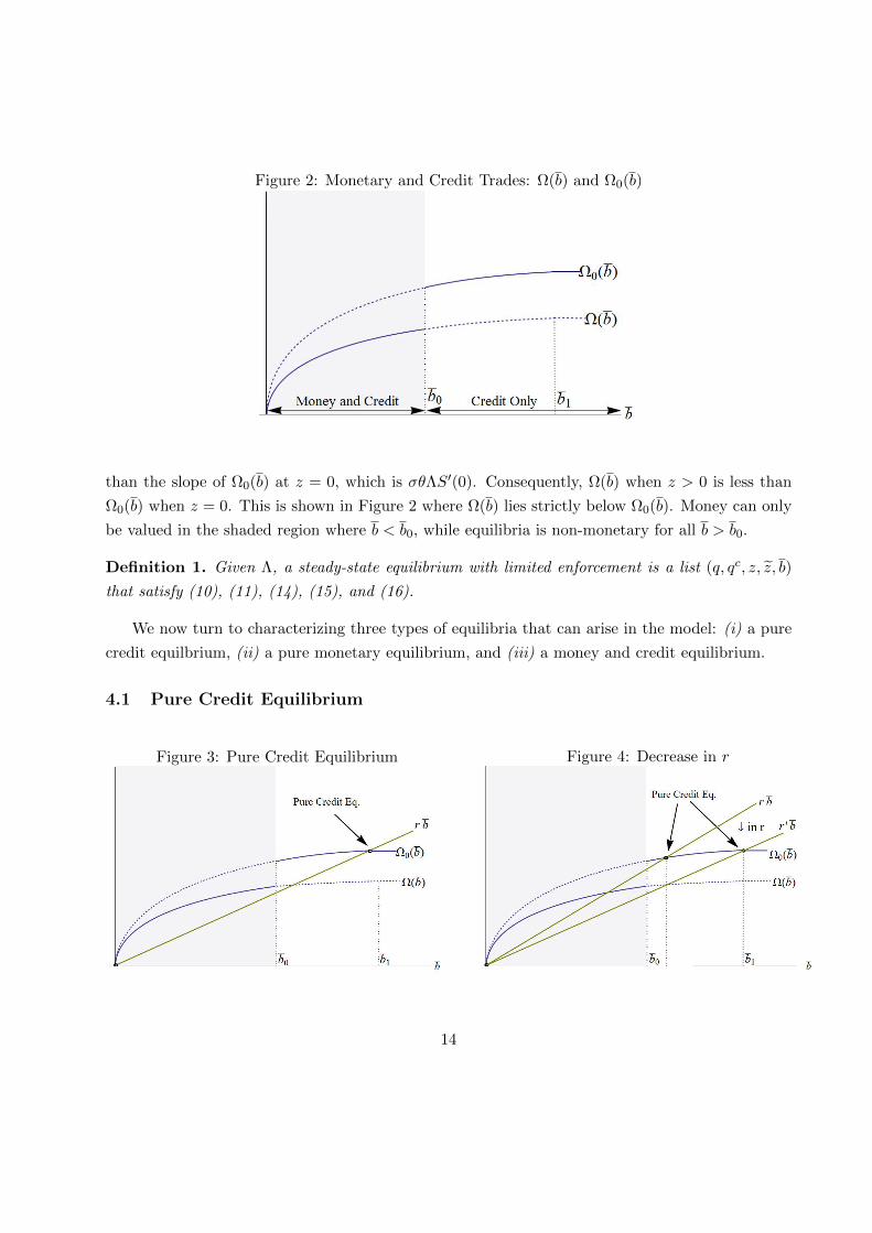
Figure 2: Monetary and Credit Trades: Ω(b) and Ω0(b)

than the slope of Ω0(b) at z = 0, which is σθΛS′(0). Consequently, Ω(b) when z > 0 is less than

Ω0(b) when z = 0. This is shown in Figure 2 where Ω(b) lies strictly below Ω0(b). Money can only

be valued in the shaded region where b < b0, while equilibria is non-monetary for all b > b0.

Definition 1. Given Λ, a steady-state equilibrium with limited enforcement is a list (q, qc, z, z, b)

that satisfy (10), (11), (14), (15), and (16).

We now turn to characterizing three types of equilibria that can arise in the model: (i) a pure

credit equilbrium, (ii) a pure monetary equilibrium, and (iii) a money and credit equilibrium.

4.1 Pure Credit Equilibrium

Figure 3: Pure Credit Equilibrium Figure 4: Decrease in r

14

A non-monetary equilibrium with credit exists when z = z = 0 and b ∈ [b0,∞). When money

is not valued (z = z = 0), the debt limit b must satisfy

rb = σθΛS(b)≡ Ω0(b). (17)

A necessary condition for there to be credit is that the slope of rb is less than the slope of Ω0(b) at

b = 0. Differentiating Ω0(b), with respect to b at b = 0 yields

∂Ω0(b)

∂b

∣∣∣∣b=0

= σθΛS′ (0)

= σΛθ

1− θ.

An equilibrium with only credit will exist if

r < σΛθ

1− θ. (18)

When the fraction of sellers accepting credit is exogenous, there exists a threshold for the fraction

of credit trades, below which b = 0. From (18), credit is feasible if

Λ >r(1− θ)σθ

≡ Λ.

Figure 3 shows the determination of the debt limit. Notice that an equilibrium without credit

always exists since b = 0 is always a solution to (16). This captures the idea that an equilibrium

without credit is self-fulfilling and can arise under the expectation that borrowers will not repay

their debts in the future.

In addition, there exists a critical value for the rate of time preference, r, below which the

debt limit stops binding and borrowers can borrow enough to purchase the first-best, q∗. The

borrowing constraint will not bind if b ≥ (1 − θ)u(q∗) + θc(q∗), in which case r must satisfy

r[(1− θ)u(q∗) + θc(q∗)] = σθΛ[u(q∗)− c(q∗)]. Hence borrowers will be unconstrained if

r ≤ σθΛ[u(q∗)− c(q∗)](1− θ)u(q∗) + θc(q∗)

≡ r.

Hence the first-best is more likely to be attained if agents are more patient, trading frictions are

small, buyers have enough market power in the DM, or the fraction of the economy with access to

record-keeping is large. Since r < σΛθ1−θ is always satisfied whenever a pure credit equilibrium exists,

the borrowing constraint binds if r < r < σΛ θ1−θ and does not bind if r < r < σΛ θ

1−θ .

15

Figure 5: Pure Monetary Equilibrium

Figure 4 depicts the pure credit equilibrium and shows the effects of a decrease in r, or as agents

become more patient. When r decreases to r′ = r, the debt limit increases to b1 and quantity traded

increases from q < q∗ to q = q∗. Intuitively, the borrowing limit relaxes as agents become more

patient since buyers can credibly promise to repay more. If on the other hand r increases above

σΛ θ1−θ , the borrowing limit is driven to zero as borrowers are not patient enough to sustain credit

use. As a result, a pure credit equilibrium will cease to exist.

More generally, Ω0(b) shifts up as the measure of sellers with access to record-keeping, Λ,

increases, trading frictions, σ−1, decrease, or the buyer’s bargaining power, θ, increases, each of

which relaxes the debt limit and thereby increasing b. Moreover, notice that in a pure credit

equilibrium, inflation has no effect on the debt limit or equilibrium allocations.

4.2 Pure Monetary Equilibrium

In a pure monetary equilibrium, money is valued (z > 0) while credit is not used (b = 0). At b = 0,

Ω(0) = 0 by Lemma 2. Further, since S(z) is concave and S′ (0) = 1(1−θ) by the Envelope Theorem,

money is valued if and only if

i = σθS′(z),

i < σθS′(0),

i <σθ

1− θ≡ i.

16

The critical value, i is the upper-bound for the cost of holding money, above which money is no

longer valued.

In addition, a pure monetary equilibrium will exist uniquely so long as credit is not feasible,

or iΛ < r, so that the slope of Ω(b) at b = 0 is less than the slope of rb. Consequently, there

exists a critical value i ≡ rΛ , below which credit is not incentive-feasible. Figure 5 plots Ω(b) as a

function of b when i < i and i < i. In that case, Ω(b) and rb intersect once at b = 0, and the unique

equilibrium is one where only money is used.

The next proposition characterizes how a key policy variable, the money growth rate γ, affects

the existence of monetary equilibrium.

Proposition 1. Define γ ≡ β(1 + i) and γ ≡ β(1 + i), where i ≡ rΛ and i ≡ σθ

1−θ . If γ < γ, then

r < σΛ θ1−θ and the following steady-state equilibria are possible:

1. If γ = β, a pure monetary equilibrium with q = q∗, z = z = (1− θ)u(q∗) + θc(q∗), and b = 0

exists uniquely.

2. If γ ∈ (β, γ), a pure monetary equilibrium with q < q∗, z = z ∈ (0, (1− θ)u(q∗) + θc(q∗)), and

b = 0 exists uniquely.

3. If γ ∈ (γ, γ), a pure monetary equilibrium coexists with a pure credit equilibrium. If b = 0,

then z = z ∈ (0, (1 − θ)u(q∗) + θc(q∗)), and q < q∗. If z = z = 0, then b > 0. If in

addition, r ∈ (0, r], equilibrium is unconstrained with qc = q∗ and b = (1 − θ)u(q∗) + θc(q∗).

If r ∈ (r,Λi), equilibrium is constrained with qc < q∗ and b < (1− θ)u(q∗) + θc(q∗).

4. If γ ≥ γ, a pure monetary equilibrium ceases to exist, and a pure credit equilibrium will exist

if Λ > Λ. If r ∈ (0, r], then qc = q∗ and b = (1− θ)u(q∗) + θc(q∗). If r ∈ (r,Λi), then qc < q∗

and b < (1− θ)u(q∗) + θc(q∗).

The first part of Proposition 1 is very intuitive and simply says that when γ = β, the rate of

return on money is high enough so that there is no need to use credit. This is because when γ, or

equivalently i, decreases, the expected surplus from defaulting increases which raises the incentive

to renege on debt repayment. This in turn tightens the credit constraint and leads the debt limit

b to fall. When γ → β or i→ 0, money becomes costless to hold and the incentive to renege is too

high to support voluntary debt repayment. Efficient monetary policy drives out credit, and money

alone is enough to finance the first-best.

In addition, the Friedman rule is sufficient but not necessary to permit the uniqueness of a

pure monetary equilibrium. Proposition 1 also shows that so long as γ < γ, credit can never be

sustained since the incentive to renege is too high. To take the most extreme case, suppose that

17

Λ = 1 so that all sellers accept credit. In that case, a pure monetary equilibrium will exist if i < r,

or equivalently, γ < γ = 1. Even though all sellers accept credit, buyers choose to only hold real

balances since the incentives to renege on debt repayment is too high.

It is possible for a pure monetary equilibrium to coexist with a pure credit equilibrium when

γ ∈ (γ, γ). In this region, the cost of money is high enough for debt repayment to be feasible and

low enough so that money can still be valued.

When γ > γ, money is too costly to hold and only credit is feasible. The first-best allocation

can be achieved provided that agents are patient enough, or if r ∈ (0, r]. This can be implemented

with any inflation rate such that γ > γ ≡ β(1 + i). In that case, equilibrium is unconstrained and

a pure credit economy ensures that agents trade the first-best level of output.

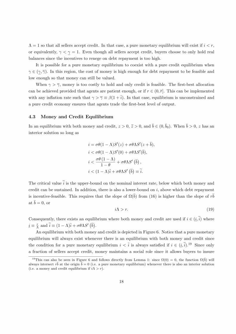
4.3 Money and Credit Equilibrium

In an equilibrium with both money and credit, z > 0, z > 0, and b ∈ (0, b0). When b > 0, z has an

interior solution so long as

i = σθ(1− Λ)S′(z) + σθΛS′(z + b),

i < σθ(1− Λ)S′(0) + σθΛS′(b),

i <σθ (1− Λ)

1− θ+ σθΛS′

(b),

i < (1− Λ)i+ σθΛS′(b)≡ i.

The critical value i is the upper-bound on the nominal interest rate, below which both money and

credit can be sustained. In addition, there is also a lower-bound on i, above which debt repayment

is incentive-feasible. This requires that the slope of Ω(b) from (16) is higher than the slope of rb

at b = 0, or

iΛ > r. (19)

Consequently, there exists an equilibrium where both money and credit are used if i ∈ (i, i) where

i ≡ rΛ and i ≡ (1− Λ)i+ σθΛS′

(b).

An equilibrium with both money and credit is depicted in Figure 6. Notice that a pure monetary

equilibrium will always exist whenever there is an equilibrium with both money and credit since

the condition for a pure monetary equilibrium i < i is always satisfied if i ∈ (i, i).19 Since only

a fraction of sellers accept credit, money maintains a social role since it allows buyers to insure

19This can also be seen in Figure 6 and follows directly from Lemma 1: since Ω(0) = 0, the function Ω(b) willalways intersect rb at the origin b = 0 (i.e. a pure monetary equilibrium) whenever there is also an interior solution(i.e. a money and credit equilibrium if iΛ > r).

18

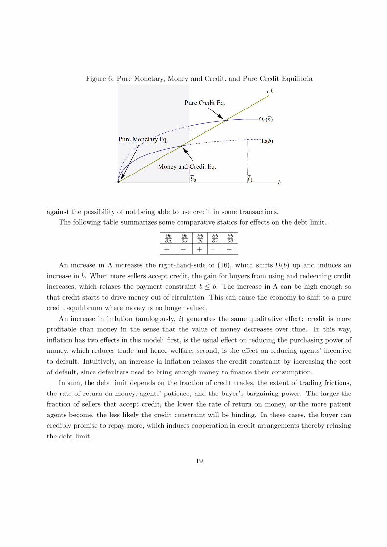
Figure 6: Pure Monetary, Money and Credit, and Pure Credit Equilibria

against the possibility of not being able to use credit in some transactions.

The following table summarizes some comparative statics for effects on the debt limit.

∂b∂Λ

∂b∂σ

∂b∂i

∂b∂r

∂b∂θ

+ + + – +

An increase in Λ increases the right-hand-side of (16), which shifts Ω(b) up and induces an

increase in b. When more sellers accept credit, the gain for buyers from using and redeeming credit

increases, which relaxes the payment constraint b ≤ b. The increase in Λ can be high enough so

that credit starts to drive money out of circulation. This can cause the economy to shift to a pure

credit equilibrium where money is no longer valued.

An increase in inflation (analogously, i) generates the same qualitative effect: credit is more

profitable than money in the sense that the value of money decreases over time. In this way,

inflation has two effects in this model: first, is the usual effect on reducing the purchasing power of

money, which reduces trade and hence welfare; second, is the effect on reducing agents’ incentive

to default. Intuitively, an increase in inflation relaxes the credit constraint by increasing the cost

of default, since defaulters need to bring enough money to finance their consumption.

In sum, the debt limit depends on the fraction of credit trades, the extent of trading frictions,

the rate of return on money, agents’ patience, and the buyer’s bargaining power. The larger the

fraction of sellers that accept credit, the lower the rate of return on money, or the more patient

agents become, the less likely the credit constraint will be binding. In these cases, the buyer can

credibly promise to repay more, which induces cooperation in credit arrangements thereby relaxing

the debt limit.

19

The next proposition summarizes the conditions under which an equilibrium with money and

credit exists and establishes a particularly interesting case where a money and credit equilibrium

ceases to exist.

Proposition 2. When i ∈ (i, i) and Λ ∈ (0, 1), a money and credit equilibrium coexists with a

pure monetary equilibrium and a pure credit equilibrium. If Λ = 1, there can either be a pure credit

equilibrium where b > 0 and z = z = 0 or a pure monetary equilibrium where b = 0 and z > 0, but

there cannot be an equilibrium where both money and credit are used.

Proof. If Λ = 1 and money is valued, (14) and (15) imply that i = σθS′[q(z+ b)] = σθS′[q(z)], or

q(z + b) = q(z). Then since z + b = z = (1 − θ)u(q) + θc(q) from the bargaining solution, the left

side of the debt limit (16) becomes −i[z − z]= −i[z − b− z] = ib. Consequently, (16) implies that

rb = ib, or b = 0.

Proposition 2 highlights an important dichotomy between monetary and credit trades when

Λ = 1: there can be trades with credit only or trades with money only, but never trades with both

money and credit. At Λ = 1, (14) and (15) implies that if money is valued, the debt limit must be

zero: z = z > 0 implies b = 0. Since buyers obtain the same surplus whether or not they default,

there cannot exist a positive debt limit that supports voluntary debt repayment. Consequently, the

debt limit is driven to zero and there cannot be a monetary equilibrium where credit is also used.

This special case also points to the difficulty of getting both money and credit to be used when

all trades are identical and record-keeping is costless: either only credit is used as money becomes

inessential, or only money is used since the incentive to renege on debt repayment is too high.

4.4 Multiple Equilibria

A particularly striking feature of the model is that there can be a multiplicity of equilibria even

without any changes in fundamentals. The next proposition establishes the possible cases for

multiple equilibria, which the remainder of this subsection discusses.

Proposition 3. When i > i, equilibrium will be non-monetary and there will either be ( i) autarky

where neither money nor credit is used if Λ < Λ or ( ii) a pure credit equilibrium if Λ > Λ. When

i < i, a pure monetary equilibrium either ( iii) exists uniquely if i < i, ( iv) coexists with a pure

credit equilibrium if i > i, or ( v) coexists with both a pure credit equilibrium and a money and

credit equilibrium if i < i < i.

Proposition 3 is illustrated in Figure 7, which plots existence conditions for different types

of equilibria in (Λ, i)-space.20 We have shown in the previous sub-sections that a necessary (but

20The types of equilibria in Figure 7 are pure credit (C) equilibrium where only credit is used, a pure monetary(M) equilibrium where only money is used, and a mixed equilibrium (B) where both money and credit are used.

20

Figure 7: Multiple Equilibria in (Λ, i)-Space

not sufficient) condition for credit is Λ > Λ. A pure monetary equilibrium will exist if and only

i < i ≡ σθ1−θ . For both money and credit to be used, it must be that i < i < i ≡ (1−Λ)i+σθΛS′

(b).

Consequently, there will be a unique equilibrium with credit only when i > i and Λ > Λ; a unique

equilibrium with money only when i < i and Λ < Λ; or multiple equilibria when i < i < i.

Figure 7 also shows how payment systems depend not just on fundamentals but also on histories

and social conventions. Suppose that inflation is initially low and the economy is in an equilibrium

where a pure monetary equilibrium coexists with a pure credit equilibrium (region M,C). As

inflation increases above i, the pure monetary equilibrium disappears and only credit is used (region

C). But when inflation goes back down to its initial level, it is possible that agents may still

coordinate on the pure credit equilibrium. The economy therefore displays hysteresis and inertia:

when there are many possible types of equilibria, social conventions and histories can dictate the

equilibrium that prevails.

When agents get less patient (r increases), both the threshold for credit to be used, Λ, and

the condition for both money and credit to be used, rΛ , increases. In Figure 7, the vertical line Λ

shifts to the right while the curve rΛ shifts up. An increase in r therefore decreases the possibility

of of any equilibrium with credit. Intuitively, less patient buyers find it more difficult to credibly

promise to repay their debts, which decreases their borrowing limit b.

5 Costly Record-Keeping

We now consider the choice of accepting credit by making Λ ∈ [0, 1] endogenous. In order to

accept credit, sellers must invest ex − ante in a costly record-keeping technology that records

21

and authenticates an IOU proposed by the buyer.21 The per-period cost of this investment is

κ > 0, which is drawn from a cumulative distribution F (κ) : R+ → [0, 1]. Sellers are heterogenous

according to their record-keeping cost and are indexed by κ.22 Hence for some sellers this cost will

be close to zero, so that they will always accept credit, while for others this cost will be very large

and they will never accept credit. The distribution of costs across sellers is known by all agents

and is assumed to be continuous.

At the beginning of each period before trades occur, sellers choose whether or not to invest

in the costly record-keeping technology. When making this decision, sellers take as given buyer’s

choice of real balances, z, and the debt limit, b. The seller’s problem is given by

max−κ+ σ(1− θ)S(z + b), σ(1− θ)S(z). (20)

According to (20), if the seller decides to invest, he incurs the disutility cost κ > 0 that allows him

to extend a loan to the buyer. In that case, the seller extracts a constant fraction (1 − θ) of the

total surplus, S(z + b) ≡ u[q(z + b)] − c[q(z + b)]. If the seller does not invest, then he can only

accept money, and gets (1− θ) of S(z) ≡ u[q(z)]− c[q(z)]. Since total surplus is increasing in the

buyer’s total wealth z+ b, S(z+ b) > S(z). Further, S(z+ b) and hence the first term in the seller’s

maximization problem (20) increases with b, and both terms of (20) increase with z.

There exists a threshold for the record-keeping cost, κ below which the seller invests in the

record-keeping technology and above which they do not invest. From (20), this threshold is given

by

κ ≡ σ(1− θ)[S(z + b)− S(z)], (21)

and gives the seller’s expected benefit of accepting credit. Since S(z + b) increases with b, the

seller’s expected benefit κ increases with b. Given κ, let λ(κ) ∈ [0, 1] denote an individual seller’s

decision to invest. This decision problem is given by

λ(κ) =

1

[0, 1]

0

if κ

<

=

>

κ. (22)

Condition (22) simply says that all sellers with κ < κ will invest in the costly record-keeping

21This cost can also reflect issues of fraud and information problems that currently permeate the credit industry.In fact, the credit card industry is facing serious challenges in the form of credit card fraud, identity theft, and theneed to secure confidential information. Besides being a costly drain on banks and retailers that accept credit, theseproblems may erode consumer confidence in the credit card industry.

22Arango and Taylor (2008) find that merchants perceive cash as the least costly form of payment while creditcards stand out as the most costly due to relatively high processing fees.

22

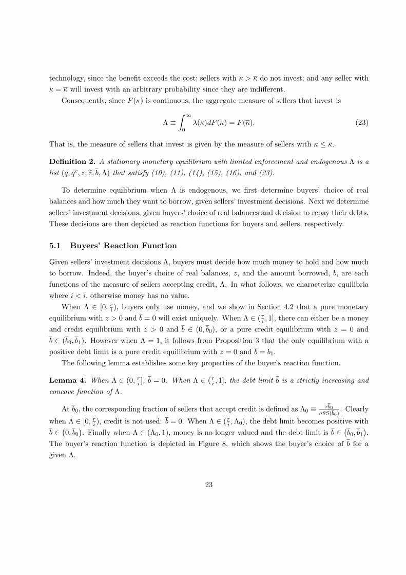
technology, since the benefit exceeds the cost; sellers with κ > κ do not invest; and any seller with

κ = κ will invest with an arbitrary probability since they are indifferent.

Consequently, since F (κ) is continuous, the aggregate measure of sellers that invest is

Λ ≡∫ ∞

0λ(κ)dF (κ) = F (κ). (23)

That is, the measure of sellers that invest is given by the measure of sellers with κ ≤ κ.

Definition 2. A stationary monetary equilibrium with limited enforcement and endogenous Λ is a

list (q, qc, z, z, b,Λ) that satisfy (10), (11), (14), (15), (16), and (23).

To determine equilibrium when Λ is endogenous, we first determine buyers’ choice of real

balances and how much they want to borrow, given sellers’ investment decisions. Next we determine

sellers’ investment decisions, given buyers’ choice of real balances and decision to repay their debts.

These decisions are then depicted as reaction functions for buyers and sellers, respectively.

5.1 Buyers’ Reaction Function

Given sellers’ investment decisions Λ, buyers must decide how much money to hold and how much

to borrow. Indeed, the buyer’s choice of real balances, z, and the amount borrowed, b, are each

functions of the measure of sellers accepting credit, Λ. In what follows, we characterize equilibria

where i < i, otherwise money has no value.

When Λ ∈ [0, ri ), buyers only use money, and we show in Section 4.2 that a pure monetary

equilibrium with z > 0 and b = 0 will exist uniquely. When Λ ∈ ( ri , 1], there can either be a money

and credit equilibrium with z > 0 and b ∈ (0, b0), or a pure credit equilibrium with z = 0 and

b ∈ (b0, b1). However when Λ = 1, it follows from Proposition 3 that the only equilibrium with a

positive debt limit is a pure credit equilibrium with z = 0 and b = b1.

The following lemma establishes some key properties of the buyer’s reaction function.

Lemma 4. When Λ ∈ (0, ri ], b = 0. When Λ ∈ ( ri , 1], the debt limit b is a strictly increasing and

concave function of Λ.

At b0, the corresponding fraction of sellers that accept credit is defined as Λ0 ≡ rb0σθS(b0)

. Clearly

when Λ ∈ [0, ri ), credit is not used: b = 0. When Λ ∈ ( ri ,Λ0), the debt limit becomes positive with

b ∈(0, b0

). Finally when Λ ∈ (Λ0, 1), money is no longer valued and the debt limit is b ∈

(b0, b1

).

The buyer’s reaction function is depicted in Figure 8, which shows the buyer’s choice of b for a

given Λ.

23

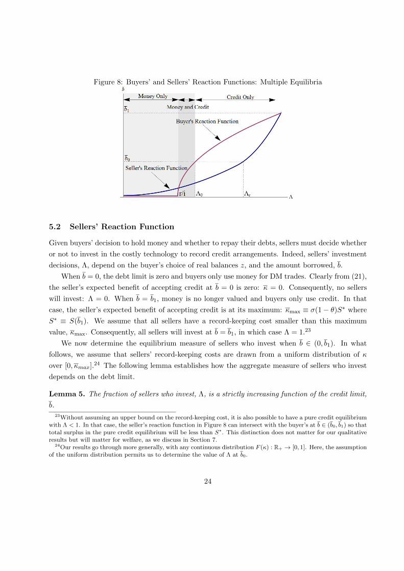
Figure 8: Buyers’ and Sellers’ Reaction Functions: Multiple Equilibria

5.2 Sellers’ Reaction Function

Given buyers’ decision to hold money and whether to repay their debts, sellers must decide whether

or not to invest in the costly technology to record credit arrangements. Indeed, sellers’ investment

decisions, Λ, depend on the buyer’s choice of real balances z, and the amount borrowed, b.

When b = 0, the debt limit is zero and buyers only use money for DM trades. Clearly from (21),

the seller’s expected benefit of accepting credit at b = 0 is zero: κ = 0. Consequently, no sellers

will invest: Λ = 0. When b = b1, money is no longer valued and buyers only use credit. In that

case, the seller’s expected benefit of accepting credit is at its maximum: κmax ≡ σ(1− θ)S∗ where

S∗ ≡ S(b1). We assume that all sellers have a record-keeping cost smaller than this maximum

value, κmax. Consequently, all sellers will invest at b = b1, in which case Λ = 1.23

We now determine the equilibrium measure of sellers who invest when b ∈ (0, b1). In what

follows, we assume that sellers’ record-keeping costs are drawn from a uniform distribution of κ

over [0, κmax].24 The following lemma establishes how the aggregate measure of sellers who invest

depends on the debt limit.

Lemma 5. The fraction of sellers who invest, Λ, is a strictly increasing function of the credit limit,

b.

23Without assuming an upper bound on the record-keeping cost, it is also possible to have a pure credit equilibriumwith Λ < 1. In that case, the seller’s reaction function in Figure 8 can intersect with the buyer’s at b ∈ (b0, b1) so thattotal surplus in the pure credit equilibrium will be less than S∗. This distinction does not matter for our qualitativeresults but will matter for welfare, as we discuss in Section 7.

24Our results go through more generally, with any continuous distribution F (κ) : R+ → [0, 1]. Here, the assumptionof the uniform distribution permits us to determine the value of Λ at b0.

24

Together, Lemma 4 and Lemma 5 allow us to characterize equilibrium as a function of the

measure of sellers who invest, Λ, and the debt limit, b.

Proposition 4. When γ ∈ [β, γ) and Λ is endogenous, there are multiple equilibria. There exists

(i) a pure monetary equilibrium with Λ = 0, z > 0, and b = 0, (ii) a pure credit equilibrium with

Λ = 1, z = 0, and b = 0; and (iii) a money and credit equilibrium with Λ < Λ0 ∈ (0, 1), z > 0, and

b > 0.

Proposition 4 is illustrated in Figure 8. The buyers’ and sellers’ reaction functions intersect

three times, corresponding to three different types of equilibria: a pure monetary equilibrium where

only money is used (Λ = 0), a money and credit equilibrium where a fraction Λ < Λ0 of sellers

accept both money and credit while the remaining (1 − Λ) sellers only accept money, and a pure

credit equilibrium where money is not valued and all sellers accept credit (Λ = 1).

Multiplicity arises through general equilibrium effects in the trading environment that produce

strategic complementarities between buyers’ and sellers’ decisions. When more sellers invest in the

costly record-keeping technology, the gain for buyers from using credit also increase. This lowers

the incentive to default and relaxes the debt limit. As a result, buyers use more credit and hold

less money. Intuitively, if it is more likely that sellers accept credit, then money is needed in a

smaller fraction of matches. So long as it is costly to hold money, buyers will therefor carry fewer

real balances. As a result, sellers have even more incentive to invest to accept credit, which in turn

raises the debt limit and hence the buyer’s real balances. These feedback effects produce network

externalities that have frequently been described to characterize retail payment systems.25

6 Welfare

We now turn to examining some of the model’s normative implications and begin by comparing

the different types of equilibria in terms of social welfare. Society’s welfare is measured as the

steady-state sum of buyers’ and sellers’ utilities in the DM:W ≡ (1−β)V b(z) + (1−β)V s(0). This

is given by

W ≡ σ[ΛS(z + b) + (1− Λ)S(z)]− k (24)

where k ≡∫ κ

0 κdF (κ) is defined as the aggregate record-keeping cost averaged across all sellers.

There can be a pure monetary equilibrium with b = 0, z > 0, and Λ = 0; a pure credit equilibrium

with b > 0, z = 0, and Λ = 1; and finally a money and credit equilibrium with b ∈ (0, b0) and z > 0

25Strategic complementarities between the seller’s decision to invest and the buyer’s choice of real balances wouldstill exist even under perfect enforcement where borrowers can always borrow enough to finance purchase of thefirst-best. See Nosal and Rocheteau (2010) for an analysis assuming loan repayments are always perfectly enforced.

25

where a fraction Λ ∈ (0, 1) of sellers accept both money and credit while the remaining (1 − Λ)

sellers only accept money. Table 1 summarizes social welfare across these types of equilibria.

Table 1: Welfare Across Equilibria

Equilibrium Welfare

Pure Monetary Wm = σS(z)

Pure Credit Wc = σS(z + b)− kMoney and Credit Wmc = σ[ΛS(z + b) + (1− Λ)S(z)]− k

For the pure credit equilibrium to dominate the pure monetary equilibrium, the aggregate

record-keeping cost must be low enough; that is, Wc >Wm if k ∈ (0, σS(z+ b)−S(z). Even with a

low-record keeping cost however, it is still possible for the welfare-dominated monetary equilibrium

to prevail due to a rent-sharing externality: since sellers must incur the full cost of adopting the

record-keeping technology but only obtains a fraction (1 − θ) of the total surplus, they fail to

internalize the full benefit of accepting credit. Consequently, there can be coordination failures

and excess inertia in the decision to accept credit, in which case the economy can end up in the

Pareto-inferior monetary equilibrium.

6.1 Optimal Monetary Policy

We now consider the issue of optimal monetary policy for the three types of equilibria examined

above. To fix ideas, we start by assuming Λ is exogenous. The presence of multiple equilibria for

the same fundamentals makes the choice of optimal policy difficult to analyze in full generality

since we must deal with the issue of equilibrium selection. In regions with multiplicity, we will

assume agents coordinate on a particular equilibrium and then analyze the optimal policy of that

equilibrium.

When i < i and i < i, agents only use money and the model reduces to the pure-currency

economy of Rocheteau and Wright (2005). In that case, social welfare is decreasing in the inflation

rate: dWmdi = σ(1 − Λ)S′(z)dzdi < 0 since from (14), dz

di = [σθ(1 − Λ)S′′(z)]−1 < 0. Since inflation

is a tax on money holdings, an increase in inflation will reduce the purchasing power of money,

and hence output and welfare. If lump-sum taxes can be enforced, the optimal policy in a pure

monetary equilibrium corresponds to the Friedman rule.

Now suppose that Λ > Λ and i ≥ i so that the economy is in a pure credit equilibrium. Since

money is not valued, inflation has no effect on welfare, irrespective of whether or not equilibrium

is efficient. When r ∈ (0, r], borrowers are patient enough to finance consumption of the first-best,

in which case welfare is at its maximum for all inflation rates. Otherwise, equilibrium is inefficient

26

and welfare is strictly dominated by welfare in a pure monetary equilibrium at the Friedman rule.

Finally, suppose that i < i < i and agents coordinate on an equilibrium where both money and

credit are used. In that case, the overall effect of inflation on welfare will be ambiguous and depend

on two effects: a real balance effect and the debt limit effect. In a money and credit equilibrium,

the effect of inflation on welfare is given by

dWmc

di= σ

ΛS′(z + b)d(z + b)

di︸ ︷︷ ︸(+)

+(1− Λ)S′(z)dz

di︸︷︷︸(–)

.In the (1−Λ) of transactions involving money only, inflating is simply a tax on buyers’ real balances,

which decreases welfare. However in the Λ of transactions with both money and credit, an increase

in inflation can be welfare improving by relaxing agents’ borrowing constraints. Intuitively, higher

inflation makes default more costly which reduces the incentive to default. The overall effect of

inflation on welfare will be positive if Λ is sufficiently large, or if Λ1−Λ > u′(q)−c′(q)

u′(qc)−c′(qc) since it can

be shown that∣∣∣d(z+b)

di

∣∣∣ > ∣∣dzdi ∣∣. Inflation can therefore have redistributive effects across agents by

lowering the consumption in the (1 − Λ) transactions with money only while raising consumption

for the fraction Λ of credit users.26

Our findings are summarized in Figures 9 and 10, which depict social welfare as a function

of the money growth rate, γ. The welfare function is continuous and concave within a particular

equilibrium, but can be discontinuous at the transition from one equilibrium to another. Figure 9

is an example where a pure monetary equilibrium exists uniquely for γ < γ and then ceases to exist

at γ when money is no longer valued. In the region where only money is used, welfare is maximized

at the Friedman rule, γ = β, in which case agents trade q∗. When γ > γ there will exist a pure

credit equilibrium. Moreover when Λ is endogenous, welfare in a pure credit equilibrium under any

inflation rate will always be dominated by a pure monetary equilibrium under the Friedman rule

since sellers must incur the real cost of technological adoption.

We now compare welfare in a pure monetary equilibrium versus an equilibrium with both

money and credit. Whenever an equilibrium with both money and credit exist, there also exists

a pure monetary equilibrium and a pure credit equilibrium, as shown in Figure 7. While there is

a multiplicity of equilibria, we assume in Figure 10 that agents coordinate on the pure monetary

equilibrium when γ ∈ [β, γ) and coordinate on the money and credit equilibrium when γ > γ. As

before, the Friedman rule maximizes welfare in the pure monetary equilibrium and implements the

26The redistributive effects of inflation are also discussed in Chiu, Dong, and Shao (2012) in a competitive environ-ment. However, competitive pricing implies that deviations from the Friedman rule is still sub-optimal and inflationis always welfare reducing, whereas inflation can be welfare improving in our model.

27

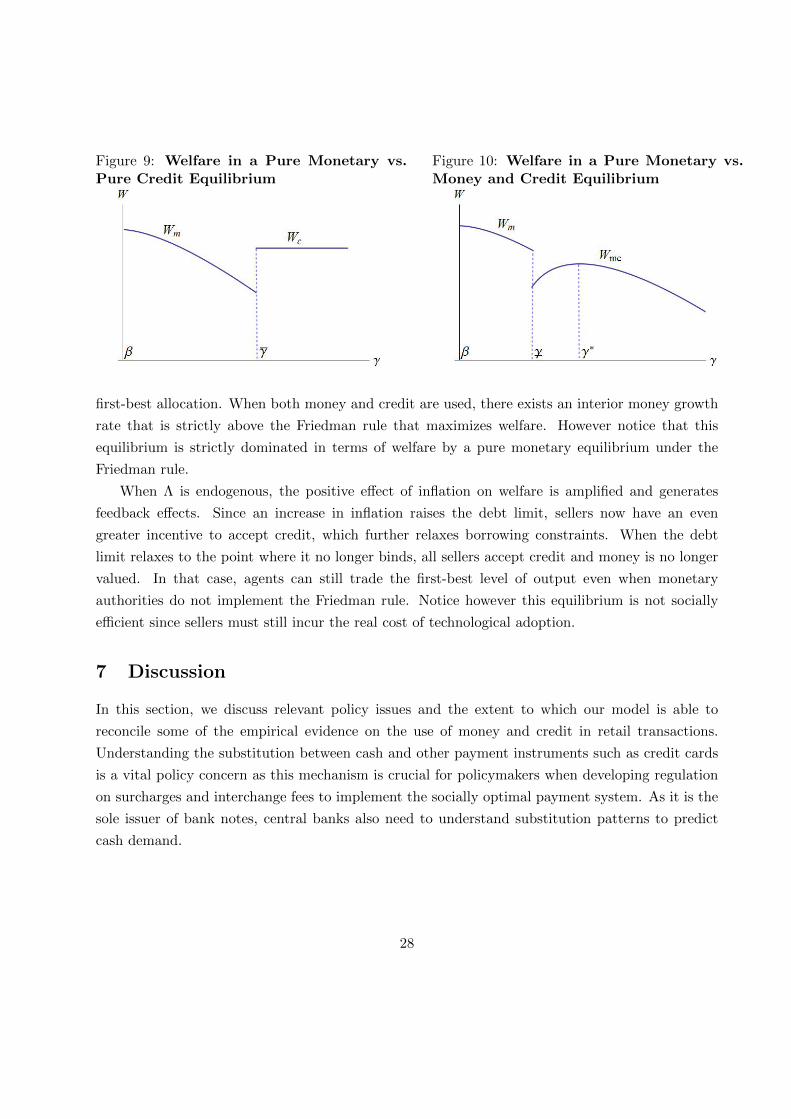
Figure 9: Welfare in a Pure Monetary vs.Pure Credit Equilibrium

Figure 10: Welfare in a Pure Monetary vs.Money and Credit Equilibrium

first-best allocation. When both money and credit are used, there exists an interior money growth

rate that is strictly above the Friedman rule that maximizes welfare. However notice that this

equilibrium is strictly dominated in terms of welfare by a pure monetary equilibrium under the

Friedman rule.

When Λ is endogenous, the positive effect of inflation on welfare is amplified and generates

feedback effects. Since an increase in inflation raises the debt limit, sellers now have an even

greater incentive to accept credit, which further relaxes borrowing constraints. When the debt

limit relaxes to the point where it no longer binds, all sellers accept credit and money is no longer

valued. In that case, agents can still trade the first-best level of output even when monetary

authorities do not implement the Friedman rule. Notice however this equilibrium is not socially

efficient since sellers must still incur the real cost of technological adoption.

7 Discussion

In this section, we discuss relevant policy issues and the extent to which our model is able to

reconcile some of the empirical evidence on the use of money and credit in retail transactions.

Understanding the substitution between cash and other payment instruments such as credit cards

is a vital policy concern as this mechanism is crucial for policymakers when developing regulation

on surcharges and interchange fees to implement the socially optimal payment system. As it is the

sole issuer of bank notes, central banks also need to understand substitution patterns to predict

cash demand.

28

7.1 Entrenchment of Cash

While consumers are adopting new instruments such as credit cards and electronic payments, they

are not necessarily discarding older ones such as cash (Schuh (2012)). Even with falling costs in

electronic record-keeping, our model predicts that agents may still coordinate on using cash due

to a hold-up externality in technological adoption. Since retailers do not receive the full surplus

associated with technological adoption, they fail to internalize the total benefit of adopting credit.

Consequently, there may be inertia in the adoption of new forms of payment.

This can explain why some merchants have been slow to adopt new technologies for accepting

credit. For example, Gerdes (2008) reports that the vast majority of card payments made within

the United States are still being made using magnetic stripe technology even though advanced chip-

based technology on “smart cards” are available. Adoption of new technologies remains limited

because merchants have not extensively adopted terminals that can read them. As we discuss more

below, policymakers must therefore remember to take into account this sluggish response when

designing policies or regulations geared towards merchant behavior.

7.2 Consumer Borrowing and Inflation

The recent recession from 2008 and 2009 in the United States provides a good recent example of our

theory in practice. During this period, the economy went from an average inflation rate of 3.85%

to deflation at -0.34% per year. Similarly, short-term interest rates available to consumers through

the rate on one-month certificates of deposit, fell from about 5% before the recession to nearly zero.

These changes in economic conditions also lead to changes in payment behavior. For the United

States, Foster, Meijer, Chuh, and Zabek (2011) find that between 2008 and 2009, cash payments

increased by 26.9%, cash holdings increased by 25.5%, while credit card payments decreased by

21.9%.27

This shift in consumer behavior during the 2008–2009 recession can be explained by our theory.

According to Proposition 1, consumer borrowing declines as inflation falls since this raises the

incentive to default. Deflation completely crowds out credit and as a result, consumers shift towards

using cash. As the evidence suggests, since both the use of cash and credit is indexed to inflation,

agents treat the two as substitutes as economic conditions change. Similarly, Kahn, Senhadji, and

Smith (2006) find that for countries with low inflation, decreases in inflation increases cash use and

decreases credit use.

27Besides deflation, the authors also discuss other factors that may explain this shift in consumer payments suchas changes in government regulations toward credit and debit cards, and changes in consumers’ assessment about thesecurity of electronic payments. Our model has a role for these factors as well, as we discuss below.

29

7.3 Hysteresis and Coordination Failures

Under certain conditions, our theory predicts that two economies with similar technologies, con-

straints, and policies can still end up with very different payment systems. Indeed, Proposition 2

and Figure 7 show that multiple equilibria can arise even without any changes in fundamentals. To

take one example, suppose there are two countries, A and B. In each country, inflation is initially

very low and all agents coordinate on an equilibrium where only money is used. Now suppose that

both countries experience a temporary period of high inflation. If inflation increases above some

threshold, the pure monetary equilibrium ceases to exist and agents turn to using credit to avoid

the inflation tax. Now suppose that in both countries, inflation goes back down to its initial low

level. It is possible that agents in country A still coordinate on using credit while agents in country

B go back to using only money. Since both outcomes are consistent with economic fundamentals,

which equilibrium an economy ends up in will depend in large part on the beliefs and expectations

of market participants.

The reason why coordination failures can arise is due to the two-sided nature of the payment

system and the beliefs of market participants. As is evident from agents’ upward-sloping reaction

functions in Figure 8, what the seller accepts affects what the buyer holds and vice versa. Coordi-

nation failures such as the kind described above can therefore arise since the maximum the buyer

can borrow and the measure of sellers that adopt the record-keeping technology are complements.28

Consequently, economies with similar fundamentals can still end up with drastically different

payment systems, some being better from society’s perspective than others. This therefore provides

rationale for policy interventions that help individuals coordinate on the better outcome. For

instance, the welfare analysis in Section 6 implies that a pure credit equilibrium dominates a pure

monetary one in terms of social welfare if inflation is high enough or the record-keeping cost is

low enough. In that case, policymakers may want to introduce mechanisms that help coordinate

agents on using credit, such as information campaigns, advertisements, or even financial literacy

programs.

7.4 Payment Regulations and Merchant Fees

Besides monetary policy intervention through changes in the nominal interest rate or inflation rate,

government policies that affect the provision of credit cards through fees and regulations also affects

consumer demand for different payment instruments. For instance, new restrictions were recently

imposed on banks and payment card networks in the United States that lead to declines in credit

28Coordination failure frequently arise in economies with frictions, and show up in many different contexts such asgoods markets and labor markets, as in Diamond (1982), Blanchard and Summer (1987), and discussed in Rocheteauand Tasci (2007).

30

card acceptance by merchants as well as decreases in credit usage by consumers. According to

Foster, Meijer, Chuh, and Zabek (2011), businesses pay merchant discount fees on credit cards to

their banks that amount to as much as 2% of total sales. Regulations that increased these fees

decreased the number of merchants that choose to accept credit, and have lead some merchants to

attempt at steering consumers toward lower cost payment instruments such as cash.29

Our theory suggests that since policy affects both retailers and consumers jointly, regulations

of this kind may have multiplier effects. For instance, suppose that policymakers pass a new law

that decreases credit card fees for merchants. In the model, a fall in κ gives merchants stronger

incentives to invest in the technology that allows for credit. At the same time, when more sellers

accept credit, the gain for buyers from using and redeeming credit also increases. This relaxes the

borrowing constraint and permits buyers to use more credit relative to cash for transactions, which

in turn amplifies the initial policy change. Through this feedback effect, policy changes such as the

wave of new regulation imposed on payment card networks in 2008 and 2009 may end up inducing

sizable shifts in consumer behavior.30

7.5 Payment Systems and Market Structure

Our framework can be used to determine how changes in market structure in retail markets impact

the adoption of payment instruments by both firms and consumers. The parameter (1 − θ) can

be interpreted as the merchant’s pricing power, or the degree of competitiveness merchants face,

which is directly related to the price mark-up: greater competition in retail markets implies θ → 1

and a mark-up close to 1. When the acceptability of credit is endogenous, the expected benefit

of investing in costly record-keeping is a decreasing function of θ.31 When θ → 1, sellers have no

pricing power and hence no long invest. More generally, increased competitiveness in the retailer

market (an increase in θ) reduces the equilibrium measure of sellers that invest and hence the

fraction of credit transactions.

This could explain why a country like the U.S. with a relatively more competitive goods markets

than the Euro Area, currently lags behind in credit-card technology. For example, the December

10, 2012 edition of Time magazine notes that: “In France and in much of the rest of the world...

banks developed chip-and-PIN, which allows merchants to authenticate transactions locally. It

became standard everywhere but in the U.S. Now we’re sub-standard.” Consequently, our theory

29Schuh and Stavins (2012) find that these costs significantly affect debit card use. Similarly, the recent increasein the cost of credit cards issued by some banks may reduce consumers’ reliance on card payments for transactions.

30For instance, the Credit Cardholder’s Bill of Rights and Regulation AA were introduced in 2008 to protectconsumers from unexpected rate increases on pre-existing credit card balances and limit the fees that reduce theavailability of credit. See Foster, Meijer, Chuh, and Zabek (2011) for more discussion on these legislative reforms.

31To verify, derive κ = σ(1− θ)[S(z + b)− S(z)] to obtain dκdθ

= −σ[S(z + b)− S(z)] < 0.

31

predicts that economies like Europe with less concentrated markets are more likely to adopt new

electronic payments than countries where the retail market is more competitive, such as the United

States.32

7.6 Payment Innovations

In many countries, there are now new mobile payments in the form of text or SMS messages that

authorizes a non-bank third party, such as a cellular phone carrier, to make a payment for the

consumer. Since this new type of mobile payment may involve short-term credit extended by a

cellular carrier or another third party, it serves the same role as credit cards that allow consumers

to “buy now and pay later” (Foster, Meijer, Chuh, and Zabek (2011)).

Perhaps the largest potential gain from these payment innovations lies in emerging markets,

where the lack of financial infrastructure makes mobile payments especially appealing (The Economist,

2012). For example, phone-based payments such as M-Pesa currency serve Kenya and several other

markets. Large credit card companies such as Visa and Mastercard have set up joint ventures with

many payment services in emerging countries such as Fundamo, which specialises in payment ser-

vices for the un-banked and under-banked, and Telefonica, which aims to boost mobile payments

across Latin America. The results from our paper suggests that in order for these innovations

to be successful, there should be more information campaigns that promote their use in order to

successfully coordinate agents on making the substitution away from cash.

8 Conclusion

As many economies now feature new forms of payment such as credit cards, smart cards, and elec-

tronic money, it is increasingly important for policymakers to understand how consumers substitute

between cash and competing media of exchange. For that purpose, we investigate the choice of

payment instruments in a simple model featuring costly record-keeping and limited commitment.

Inflation triggers agents to substitute from money to credit for two reasons: a higher inflation

rate both lowers the rate of return on money and makes default more costly, which relaxes agents’

borrowing limits.

Our model also highlights a strategic complementarity between consumers’ credit limit and

retailers’ decision to invest. Multiple equilibria and coordination failures can therefore arise due to

the two-sided market nature of payment systems. This poses new challenges for policymakers and

32Bayoumi, Laxton, and Pesenti (2004) estimate an average price mark-up of 1.30 for the Euro Area and 1.16 forthe U.S., which reflects a relatively more competitive goods market in the United States. Stavins (2003) presents asimilar market structure argument regarding the market for electronic check products.

32

we discuss some mechanisms such as information campaigns and financial literacy programs that

can help coordinate society on the socially preferred outcome. Our theory also suggests that future

research should include more empirical studies on consumer preferences and merchant adoption

to help policymakers enact the most beneficial regulations, laws, and educational programs that

protect and support both consumer’s and firm’s payment choices.

33

References

Rao Aiyagari, and Stephen Williamson (1999): “Credit in a Random Matching Model with Private

Information.” Review of Economic Dynamics, 36–64.

Akers, Douglas, Jay Golter, Brian Lamm, and Martha Sol (2005): “Overview of Recent Devel-

opments in the Credit Card Industry.” FDIC Banking Review.

Alvarez, Fernando and Urban J. Jermann (2000): “Efficiency, Equilibrium, and Asset Pricing

with Risk of Default.” Econometrica, 68, 775–797.

Andolfatto, David (2008): “The Simple Analytics of Money and Credit in a Quasi-Linear En-

vironment.” Working paper, ch. 6.

Antinolfi, Gaetano, Costas Azariadis, James Bullard (2009): “The Optimal Inflation Target in

an Economy with Limited Enforcement.” Washington University in St. Louis, Manuscript, 2007.

Arango, Carlos, Dylan Hogg, and Alyssa Lee: “Why is Cash (Still) So Entrenched? Insights

from the Bank of Canada’s 2009 Methods-of-Payment Survey.” Bank of Canada working paper.

Arango, Carlos, Kim Huynh, and Leonard Sabetti (2009): “How Do You Pay? The Role of

Incentives at the Point of Sale.” Bank of Canada working paper, 2011-23.

Arango, Carlos and Varya Taylor (2008): “Merchants’ Costs of Accepting Means of Payment:

Is Cash the Least Costly?” Bank of Canada Review Article: Bank of Canada Review - Winter

2008-2009.

Bethune, Zachary, Guillaume Rocheteau, and Peter Rupert (2013): “Unemployment and House-

hold Unsecured Debt.” Working paper.

Bewley, T. (1980): “The Optimum Quantity of Money.” In Kareken and Wallace, eds., Models

of Monetary Economies, Federal Reserve Bank of Minneapolis.

Blanchard, Olivier and Lawrence Summers (1987): “Fiscal Increasing Returns, Hysteresis, Real

Wages and Unemployment.” European Economic Review, vol. 31, 543-566.

34

Bullard, James, Gaetano Antinolfi, and Costas Azariadis (2008): “The optimal inflation target

in an economy with limited enforcement.” Speech, Federal Reserve Bank of St. Louis, issue Oct 2.

Cavalcanti, R. and N. Wallace (1999): “Inside and Outside Money as Alternative Media of

Exchange.” Journal of Money, Credit and Banking, 31, 443-457.

Chakravorti, S. and T. To (2007): “A Theory of Credit Cards.” International Journal of Indus-

trial Organization, 25(3), 583-595

Chiu, Jonathan, Mei Dong, and Enchuan Shao (2012): “On the Welfare Effects of Credit Ar-

rangements.” Bank of Canada working paper 2012-43.

Diamond, Peter (1982): “Aggregate Demand Management in Search Equilibrium.” Journal of

Political Economy, vol. 90, 881-94.

Dong, Mei (2011): “Money and Costly Credit.” Working paper.

Duca, John V and William C. Whitesell (1995): “Credit Cards and Money Demand: A Cross-

sectional Study.” Journal of Money, Credit and Banking, 27 (2), 604-623.

Dutta, Rohan (2012): “Bargaining with Revoking Costs.” Games and Economic Behavior, Vol-

ume 74, Issue 1, 144-153.

Ernst and Young (1996): “Survey of Retail Payment Systems.” Chain Store Age, January.

Federal Reserve Payments Study (2010): “The 2010 Federal Reserve Payments Study: Non-

Cash Payment Trends in the United States: 2006 2009.”

Foster, Kevin, Erik Meijer, Scott Schuh, and Michael Zabek (2011): “The 2009 Survey of Con-

sumer Payment Choice.” Federal Reserve Bank of Boston Public Policy Discussion Papers.

Fung, Ben, Kim Huynh, and Lenoard Sabetti (2012): “Impact of Retail Payment Innovations

on Cash Usage.” Bank of Canada Working Paper 2012-14.

35

Gerdes, Geoffrey , Jack Walton II, May Liu, and Darrel Parke (2005): “Trends in the use of

Payment Instruments in the United States.” Federal Reserve Bulletin, vol. 91, no. 2, pp. 180-201.

Gerdes, Geoffrey (2008): “Recent Payment Trends in the United States.” Federal Reserve Bul-

letin, vol. 94, pp. A75-A106.

Gomis-Porqueras, Pedro and Daniel Sanches (2011): “Optimal Monetary Policy in a Model of

Money and Credit.” Journal of Money, Credit, and Banking, forthcoming.

Gomis-Porqueras, Pedro and Peralta-Alva, Adrian (2010): “Optimal Monetary and Fiscal Poli-

cies in a Search Theoretic Model of Monetary Exchange.” European Economic Review.

Gomis-Porqueras, Pedro, Peralta-Alva, Adrian, and Christopher Waller (2011): “Quantifying

the Shadow Economy: Measurement with Theory.” Federal Reserve Bank of St. Louis working

paper.

Gowrisankaran, Gautam and Joanna Stavins (2004): “Network Externalities and Technology

Adoption: Lessons from Electronic Payments. RAND Journal of Economics. vol. 35, no. 2, 260–

276.

Gu, Chao and Randall Wright (2011): “Endogenous Credit Cycles.” Working paper.

Hoenig, Thomas (1995): “The Evolution of the Payments System: A U.S. Perspective.” Federal

Reserve Bank of Kansas City working paper.

Humphrey, D., L. Pulley, and J. Vesala (1996): “Cash, Paper and Electronic Payments: A

Cross-Country Analysis.” Journal of Money, Credit, and Banking, 28, 914–934.

Kehoe, Timothy and David Levine (1993): “Debt-Constrained Asset Markets.” Review of Eco-

nomic Studies, 60(4), 865–888.

Khan, Mohsin, Abdelhak Senhadji, and Bruce Smith (2006): “Inflation and Financial Depth.”

Macroeconomic Dynamics, 10, 165-182.

Klee, Elizabeth (2006): “Paper or Plastic? The Effect of Time on Check and Debit Card Use

36

at Grocery Stores.” Federal Reserve Board Finance and Economics Discussion Series: 2006-02.

Kocherlakota, Narayana (1998): “Money Is Memory.” Journal of Economic Theory,vol. 81(2),

232-251.

Kocherlakota, Narayana and Neil Wallace (1998): “Incomplete Record-Keeping and Optimal

Payment Arrangements.” Journal of Economic Theory, vol. 81(2), 272-289.

Koulayev, Sergei, Marc Rysman, Scott Schuh, and Joanna Stavins (2012): “Explaining Adop-

tion and Use of Payment Instruments by U.S. Consumers.” Federal Reserve Bank of Boston Working

Paper No. 12-14.

Lagos, Ricardo and Randall Wright (2005): “A Unified Framework for Monetary Theory and

Policy Analysis.” Journal of Political Economy, 113 (3), 463-484.

McAndrews, James (1997): “Network Issues and Payment Systems.” Federal Reserve Bank of

Philadelphia Business Review, 15-25.

Mills, David C., Jr. (2007): “A Model in which Outside and Inside Money are Essential.”

Macroeconomic Dynamics, vol. 11, no. 3, 347–366.

Nosal, Ed and Guillaume Rocheteau (2011): Money, Payments, and Liquidity. MIT Press.

Rochet, Jean-Charles and Jean Tirole (2002): “Cooperation Among Competitors: Some Eco-

nomics of Payment Card Associations.” RAND Journal of Economics, 33, 549–570.

Rocheteau, Guillaume and Murat Tasci (2007): “Coordination Failures in the Labor Market.”

Federal Reserve Bank of Cleveland Economic Commentary.

Rysman, Marc (2009): “The Economics of Two-Sided Markets.” Journal of Economic Perspec-

tives, volume 23, 3, 125–143.

Sanches, Daniel and Stephen Williamson (2010): “Money and Credit with Limited Commit-

ment and Theft.” Journal of Economic Theory, Volume 145, 1525-1549.

37

Schreft, Stacey (1992): “Transaction Costs and the Use of Cash and Credit.” Economic Theory,

2, 283–296.

Schreft, Stacey (2006): “How and Why Do Consumers Choose Their Payment Methods?” Fed-

eral Reserve Bank of Kansas City working paper.

Schuh, Scott (2012): “Consumer Payment Choice: A Central Bank Perspective.” Federal Re-

serve Bank of Boston presentation, 2012 Little Client Conference.

Schuh, Scott and Joanna Stavins (2012): “How Consumers Pay: Adoption and Use of Pay-

ments.” Federal Reserve Bank of Boston Working Paper Series, no. 12-2.

Shi, Shouyong (1996): “Credit and Money in a Search Model with Divisible Commodities.”

Review of Economic Studies, 63, 627–652.

Stavins, Joanna (2003): “Network Externalities in the Market for Electronic Check Payments.”

New England Economic Review.

Stavins, Joanna (2011): “Consumer Payments Cards: Lessons from the U.S. Experience.” Fed-

eral Reserve Bank of Boston presentation at Cards and Payments Australasia, Sydney, Australia.

The Economist (2012): “War of the Virtual Wallets.” November 17, 2012 print edition.

Time Magazine (2013): “The Chips Are Down. Why the U.S. Lags in Credit-Card Technology.”

December 10, 2012 print edition.

Townsend, Robert (1980): “Models of Money with Spatially Separated Agents.” in J. Kareken,

N. Wallace (Eds.), Models of Monetary Economies, Federal Reserve Bank of Minneapolis, Min-

neapolis, 265-304.

Townsend, Robert (1989): “Currency and Credit in a Private Information Economy.” Journal

of Political Economy, 97, 1323-1344.

Turban, Efraim (2008): “Electronic Payment Systems.” Pearson Prentice Hall, Electronic Com-

merce.

38

Wakamori, Naoki and Angelika Welte (2012): “Why Do Shoppers Use Cash? Evidence From

Shopping Diary Data.” Bank of Canada working paper 2012-24.

Williamson, Stephen (1999): “Private Money.” Journal of Money, Credit and Banking, 31, 469-

491.

Williamson, Stephen (2004): “Limited Participation, Private Money, and Credit in a Spatial

Model of Money.” Economic Theory, 24, 857-875.

Wright, Julian (2002): “Why do Firms Accept Credit Cards?” Mimeo, University of Auckland.

Wright, Julian (2003): “Pricing in Debit and Credit Card Schemes.” Economics Letters.

39

Appendix

Concavity of Buyer’s Objective Function

The buyer’s objective function is

Ψ(z) = −iz + σθΛ[u(qc)− c(qc)] + σθ(1− Λ)[u(q)− c(q)],

where qc and q are given by z + b = (1− θ)u(qc) + θc(qc) and z = (1− θ)u(q) + θc(q), respectively,

and b is given by (16). The partial derivative of the buyer’s objective function with respect to the

choice of real balances are

Ψ′(z) = −i+ σθΛ

[u′(qc)− c′(qc)

θc′(qc) + (1− θ)u′(qc)

]+ σθ(1− Λ)

[u′(q)− c′(q)

θc′(q) + (1− θ)u′(q)

],

if z + b < (1 − θ)u(q∗) + θc(q∗) and Ψ′(z) = 0 if z + b ≥ (1 − θ)u(q∗) + θc(q∗). Consider the case

where z + b < (1− θ)u(q∗) + θc(q∗) and hence qc < q∗ and q < q∗. The second partial derivative is

Ψ′′(z) = σθ[Λ∆c + (1− Λ)∆] < 0,

where ∆c = u′′(qc)c′(qc)−u′(qc)c′′(qc)[θc′(qc)+(1−θ)u′(qc)]3 and ∆ = u′′(q)c′(q)−u′(q)c′′(q)

[θc′(q)+(1−θ)u′(q)]3 . Hence for all (z, b) such that b solve

(16) and z + b < (1− θ)u(q∗) + θc(q∗), the objective function Ψ(z) is strictly concave.

Proof of Lemma 1

The borrowing limit, b, is determined in order to satisfy the buyer’s incentive constraint to volun-

tarily repay his debt in the CM. The buyer will repay his debt if

W b (z,−b) > W b (z) ,

where W b(z,−b) is the value function of a buyer who chooses to repay his debt at the beginning

of the CM, and W b(z) is the value function of a buyer who chooses to default. By the linearity of

W b, the value function of a buyer who repays his debt in the CM is

W b (z,−b) = z − b+W b (0, 0) .

40

On the other hand, the value function of a buyer who defaults, W b(z) must satisfy

W b (z) = z + T + maxz′≥0

−γz′ + βV b

(z′)

= z + W b(0)

since by defaulting, he is excluded from the use of credit for all future trades and can only use z

real balances for trades in the next DM. As a result, a buyer will repay his debt if

W b (z,−b)− W b (z) ≥ 0,

W b (0, 0)− W b (0) ≥ b,

b ≥ b,

where b ≡W b (0, 0)− W b (0) is the endogenous debt limit determined such that buyers will always

repay their debt. Therefore, the repayment constraint takes the form of an upper bound on credit

use. To obtain the expression for b, we now determine W b (0, 0) − W b (0). The value functions of

a buyer who does not default in the CM can be rewritten as

W b (0, 0) = T + maxz≥0

−γz + βV b (z)

= T + max

z≥0

−γz + β

[σ (1− Λ) θS (z) + σΛθS

(z + b

)+ z +W b (0, 0)

],

where S (z) ≡ u [q (z)] − c [q (z)] is the total trade surplus when sellers only accept money, and

S(z + b

)≡ u

[q(z + b

)]− c

[q(z + b

)]is the total trade surplus when both money and credit are

accepted. Rearranging and dividing both sides of the equality by β results in

(1− β)

βW b (0, 0) =

T

β+ max

z≥0

−(γ − β)

βz + σθ

[(1− Λ)S (z) + ΛS

(z + b

)].

Similarly, the value functions of a buyer who defaults in the CM can be rewritten as

W b (0) = T + maxz≥0

−γz + βV b (z)

= T + max

z≥0

−γz + β

[σθS (z) + z + W b (0)

],

where z > 0 solves

i = σθ[u′(q(z))− c′(q(z))]

θc′(q(z)) + (1− θ)u′(q(z)), (25)

41

since a buyer who defaults can only use money irrespective of what the seller accepts. Rearranging

and dividing both sides of the equality by β results in

(1− β)

βW b (0) =

T

β+ max

z≥0

−(γ − β)

βz + σθS (z)

.

Therefore, the debt limit, b, must satisfy

(1− β)

βb =

(1− β)

β

[W b (0, 0)− W b (0)

].

Substituting in the expressions for W b(0, 0) and W b(0) then leads to the following expression for b:

rb = maxz≥0

−iz + σθ

[(1− Λ)S (z) + ΛS

(z + b

)]−max

z≥0−iz + σθS (z) ≡ Ω(b) (26)

where r = 1−ββ .

Proof of Lemma 2

First, we show that Ω(0) = 0. If b = 0, it must be that z = z since

−iz + σθS(z) = −iz + σθS(z).

As a result, Ω(0) = 0. Next, to verify that Ω(b) is increasing in b, differentiate Ω(b) with respect

to b to obtain

∂Ω(b)

∂b= σθΛS′

(z + b

)= σθΛ

u′ (qc)− c′(qc)(1− θ)u′ (qc) + θc′(qc)

> 0,

where qc ≡ q(z + b) is output traded when the seller accepts both money and credit and z > 0

satisfies

i = σθ[(1− Λ)S′ (z) + ΛS′

(z + b

)].

42

The slope of Ω(b) with respect to b is strictly positive for all b < (1− θ)u(q∗) + θc(q∗) and becomes

zero when b > (1− θ)u(q∗) + θc(q∗). Further, the slope of Ω(b) at b = 0 is

∂Ω(b)

∂b

∣∣∣∣b=0

= σθΛS′ (z)

= iΛ ≥ 0.

A necessary for a monetary equilibrium with a positive debt limit is that the slope of rb from (16)

is less than the slope of Ω(b) at b = 0. Consequently a monetary equilibrium with b > 0 will exist

so long as r < Ω′(b) = iΛ.

Next, Ω(b) is concave since total surplus S(z + b) as a function of the buyer’s liquid wealth,

z + b, is concave and strictly concave if z + b < θc(q∗) + (1− θ)u(q∗). Consequently,

∂2Ω(b)

∂b2 =

∂[σθΛS′(z + b)]

∂b

= σθΛS′′(z + b) ≤ 0,

since S′′(z + b) ≤ 0. Finally, Ω(b) is continuous for all z > 0, and for i > 0, the solution to (14)

and (15) must lie in the interval [0, z∗]. Then from the Theorem of the Maximum, there exists a

solution to (14) and (15), and consequently (16).

Proof of Lemma 4

First we differentiate (16) to obtain

rdb = σθ[−S(z)dΛ + S(z + b)dΛ + ΛS′(z + b)db

],

db

dΛ=σθ[S(z + b)− S(z)

]r − σθΛS′(z + b)

> 0,

since S(z + b) > S(z) and r > σθΛS′(b0). Next, we verify that b is a concave function of Λ:

d2b

dΛ2=− (σθ)2 [S(z + b)− S(z)

]S′(z + b)[

r − σθΛS′(z + b)]2 < 0

since S′(z + b) > 0. Therefore, d2bdΛ2

∣∣∣b<b0

> d2bdΛ2

∣∣∣b0.

43

Proof of Lemma 5

We first establish sellers’ investment decisions at b = b0 where money is not valued. For a given

b = b0, the fraction of sellers who invest in the record-keeping technology depends on the expected

benefit of accepting credit when money is not used in trade by buyers:

κ0 ≡ σ(1− θ)S(b0).

Clearly, a seller will invest so long as the expected benefit of doing so outweighes the cost: κ0 > κ.

Assuming a uniform distribution of κ over [0, κmax], the aggregate measure of sellers who invest at

b0 is given by Λs = S(b0)S∗ , where S∗ ≡ S(b1) is the maximum surplus obtained when q = q∗.

For all b ∈ (b0, b1), the expected benefit of investing is

κ = σ(1− θ)S(b)

where κ > κ0. Then since Λ is increasing in κ, it follows that Λ > Λs. Moreover, the expected

benefit of investing is a strictly increasing function of the debt limit, b: dκdb

∣∣b>b0

> 0 and d2κ

db2

∣∣b>b0

< 0.

To verify, differentiate κ to obtain

dκ

db

∣∣∣∣b>b0

= σ(1− θ)S′(b) > 0

since S′(b) > 0. Then differentiating again, it is easy to see that

d2κ

db2

∣∣∣∣b>b0

= σ(1− θ)S′′(b) ≤ 0

since S′(b) ≤ 0. Next, for all b ∈ (0, b0), the expected benefit of investing is

κ = σ(1− θ)[S(z + b)− S(z)].

Consequently, κ < κ0 and Λ < Λs. In this region, the expected benefit of investing is also an

increasing function of the debt limit, b. To verify, we differentiate to obtain

dκ

db

∣∣∣∣b<b0

= σ(1− θ)S′(z + b) +

[S′(z + b)− S′(z)

] dzdb

.

44

Then using the first order condition (14),

i = σθ[(1− Λ)S′(z) + ΛS′(z + b)

],

we obtaindz

db= − 1

1 + (1−Λ)S′′(z)

ΛS′′(z+b)

< 0

since S′′(z) ≤ 0 and S′′(z + b) ≤ 0. Consequently, dκdb

∣∣b<b0

> 0.33

33We do not determine d2κ

db2 when b < b0 since this will not affect our results and will depend on third derivative

S′′′(z + b), which we do not know the sign of.

45