Coastal Engineering

1

Professor A G L Borthwick Hilary Term 2010

Paper C2A: STRUCTURES AND FLUIDS

4CE16: COASTAL ENGINEERING

Lecture 1 Coastal Hydrodynamics I

1.0 Textbooks

(1) Dean, R.G. and Dalrymple, R.A. (1991) Water Wave Mechanics for

Engineers and Scientists, World Scientific Press, ISBN 981-02-0420-5.

(2) Komar, P.D. (1998) Beach Processes and Sedimentation. 2nd

Edition. Prentice-Hall, ISBN 0-13-754938-5.

1.1 Introduction

The Shore Protection Manual defines coastal engineering as “the

application of the physical and engineering sciences to the planning,

design, and construction of works to modify or control the interaction of

the air, sea, and land in the coastal zone for the benefit of man and the

enhancement of natural shoreline resources”.

Wind and wave forces weather the coastline, reducing rocky headlands

to boulders, pebbles and sand. Waves and currents transport

sediments, and cause morphological change through accretion and

erosion. A long-term equilibrium is often reached. Although severe

storms can greatly change a beach profile, there is later a tendency for

the original profile to re-establish itself.

When coastal engineering works are undertaken, the transport

processes may be disrupted. The resultant effects can negate the

Coastal Engineering

2

original engineering work and also damage nearshore equilibrium

systems in neighbouring bays. Examples include dredging activities that

lead to additional settlement of suspended sediment, and beach groynes

which then cause erosion of adjacent beaches by cutting off the

longshore supply of sand.

Coastal flows are driven by tides, wind, waves and currents. Tides

determine the mean water depths. Winds generate ocean swell (waves)

and currents. Waves are modified by the coastal topography as they

head towards the shore. They shoal, refract, diffract, reflect and break.

Energy is dissipated through wave breaking, bed friction and turbulence.

Shoaling causes the wave height to increase as the wave speed

reduces in progressively shallow waters. Refraction occurs when the

incident wave direction is non-orthogonal to the bed contours, and the

wave front bends due to relative differences in speed. Hence, the wave

fronts become more parallel to the shore. The wave height distribution

is also affected by refraction because of changes in the distance

between adjacent wave orthogonals. Diffraction alters wave heights

due to energy transfer from high energy passing waves to the low

energy region in the lee of a large obstacle, such as a breakwater.

Reflection occurs when waves collide with a barrier, depending on its

permeability. At a rubble-mound breakwater, the wave amplitude is

partly reflected, transmitted and absorbed.

At a limiting height to depth ratio, waves become unstable and break.

The broken waves run up the beach as a bore. Longuet-Higgins and

Stewart have shown that excess momentum flux of the waves (termed

radiation stress) leads to set-up (rise of mean water level) at the land-

Coastal Engineering

3

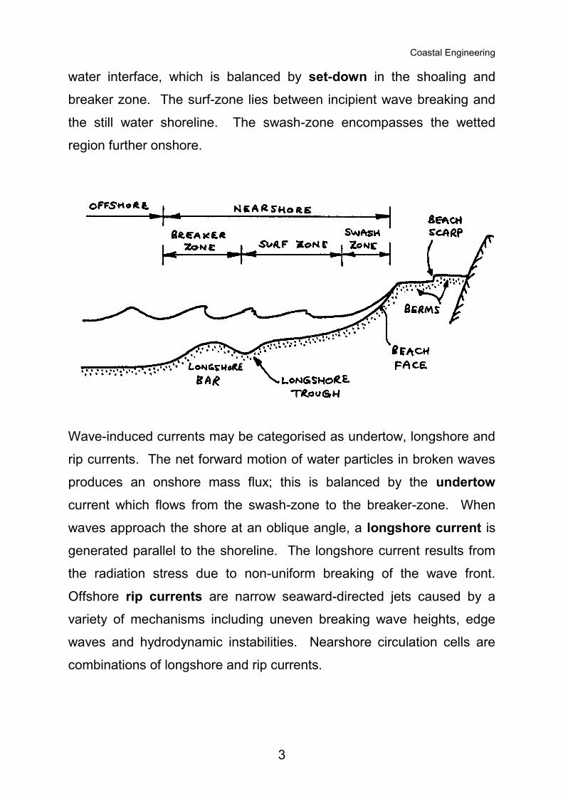
water interface, which is balanced by set-down in the shoaling and

breaker zone. The surf-zone lies between incipient wave breaking and

the still water shoreline. The swash-zone encompasses the wetted

region further onshore.

Wave-induced currents may be categorised as undertow, longshore and

rip currents. The net forward motion of water particles in broken waves

produces an onshore mass flux; this is balanced by the undertow

current which flows from the swash-zone to the breaker-zone. When

waves approach the shore at an oblique angle, a longshore current is

generated parallel to the shoreline. The longshore current results from

the radiation stress due to non-uniform breaking of the wave front.

Offshore rip currents are narrow seaward-directed jets caused by a

variety of mechanisms including uneven breaking wave heights, edge

waves and hydrodynamic instabilities. Nearshore circulation cells are

combinations of longshore and rip currents.

Coastal Engineering

4

Breaking waves stir sediments into suspension. Sediment transport is

primarily by wave-induced currents.

1.2 Tides

Tides cause the mean sea level to vary. Tidal harmonic analysis

involves fitting a Fourier cosine series to tidal observations at a given

location:

)cos()(1

0 nn

N

n

np tat

where p is the predicted tidal elevation at time t, 0 is the mean sea

level relative to some reference datum (obtained by averaging the

observed values), an and n are the amplitude and phase of the n-th

constituent at the location in question, n is the frequency of the n-th

constituent (determined from astronomical theory by considering solar

and planetary angular speeds) and N is the number of constituents.

Values of an and n are determined by regression analysis.

Tidal response models use Fourier transfer functions which relate input

solar and lunar gravitational potentials to output tidal heights at given

frequencies.

Land masses cause tidal behaviour to be modified. Seiching effects

may occur in an enclosed sea, such as the North Sea. Converging

coastlines amplify the tidal range. Coriolis forces further complicate the

co-tidal patterns. For example, the English Channel and North Sea

Coastal Engineering

5

contain several amphidromic points of zero tidal amplitude, around

which high amplitude tides rotate. With offshore tidal boundary

conditions, a numerical model can be developed based on the (long

wave) shallow water equations to represent the effects of coastline,

bathymetry, bed friction, wind stresses, etc. Note that the behaviour of a

tide is essentially that of a very long period free surface gravity wave.

1.3 Waves Without Currents

Assume that sea water is irrotational, inviscid and incompressible and

the waves are regular and of small amplitude. We choose horizontal

coordinate axes such that x is measured in the onshore direction and y

is longshore. The waves have period T corresponding to the wave

angular frequency ω = 2π/T. The local wave number vector is

sincos kk jik where θ is the wave angle measured anticlockwise

from the onshore x-direction. The magnitude of the wave number

vector, k, may be estimated from the linear dispersion equation,

)tanh(2 kdgk

where the local mean water depth hd ; h is the still water depth

and is the set-up. Note that 2k where is the wave length.

The individual wave celerity, c, and the wave group celerity, cg, are given

by

Tkc

and nc

kcg

d

d where

)2sinh(

21

2

1

kd

kdn .

Coastal Engineering

6

The velocity potential is

Skd

dzkAgcos

)cosh(

)(cosh

where A is the wave

amplitude, g is gravitational acceleration, and z is distance vertically

upwards from mean water level. The phase function is xk tS

where yx jix .

The water particle kinematics are obtained from

wvu ,, and wvut

wvu ,,,,

where zyx

kji .

Writing out the particle velocity components in full,

cos)sincossin(

)cosh(

)(coshkykxt

kd

dzkgAku

,

sin)sincoscos(

)cosh(

)(coshkykxt

kd

dzkgAkv

,

)sincoscos(

)cosh(

)(sinh

kykxt

kd

dzkgAkw

.

Note that in shallow water, where 25/1/ d , kdkd )tanh( and the

linear dispersion equation simplifies to give

gdc .

Coastal Engineering

7

1.4 Conservation of Waves

Consider the phase function xk tS . After differentiation,

Shk and t

S

,

where the horizontal gradients are given by

yx

jih .

By definition,

0hh

t

SS

t .

Substituting from above,

0h

t

k

which is the wave conservation equation. This indicates that the wave

period is uniform spatially (regardless of the bed topography), provided

the wave field is at steady-state.

1.5 Refraction

The wave number vector is irrotational because k is equal to the

gradient ( h ) of a scalar (-S). Its curl is zero, and so

0h k .

Coastal Engineering

8

Expanding this out in full, we have the ray equation

0cossin

k

yk

x .

This is usually either solved numerically or by ray tracing approaches to

predict modifications to the wave angle as the mean water depth

changes.

For a straight beach of constant slope (hence parallel bed contours), the

ray equation simplifies to

0sind

dk

x or constantsin k .

For a steady-state wave field, ω is constant (wave conservation eqn), we

have

constantsin

sin c

k

.

This may be written as Snell’s law

oo sin

sin

c

c

where co and θo refer to the offshore wave celerity and the offshore wave

angle.

Coastal Engineering

9

For non-uniform bed contours, the wave front direction may be

estimated using ray tracing techniques. First, the ray equation is

rewritten

0cossinsincos

y

k

x

k

yxk

.

Change to a local co-ordinate system ns ˆ,ˆ where s is tangential and n

is normal to the wave direction. Hence,

sinˆcosˆ nsx and cosˆsinˆ nsy

Applying the chain rule,

yxs

sincos

ˆ and

yxn

cossin

ˆ .

By inspection, the ray equation becomes

n

c

cn

k

ks ˆ

1

ˆ

1

ˆ

.

The ray tracing procedure is: (1) plot depth contours (smoothing out

major irregularities); (2) start rays at equal spacings offshore ( 2/od );

(3) extend each ray (in wave direction) to first depth contour; and (4) for

each ray, in turn: (i) calculate local wave number k and hence wave

celerity c, (ii) use Snell’s law to calculate the refracted wave angle

relative to the normal to the bed contour and (iii) extend ray to next

contour, and return to (i).

Coastal Engineering

10

1.6 Conservation of Energy: Shoaling and Refraction

Consider waves at zero incidence to the shore without currents. The

total energy per wave per unit crest width is

0 0

2

0

22

8

1dd

1dd

2

1Hgxzzgxz

wuE

h

in which is the wave free surface elevation above still water level.

Note that the potential energy term is integrated from 0 to assuming

that the potential energy of the undisturbed water is zero. Energy flux,

F , is the rate at which energy is transmitted by waves. It is determined

as the rate of work done by dynamic pressure per unit width of wave.

Hence,

T

h

tzuzgwupT

F

0

22 dd2

11

where p is the pressure, u and w are horizontal and vertical water

particle velocity components. Using linear wave theory (and so

linearising the above equation),

gCEF .

Hence, wave energy is propagated at the wave group celerity, cg.

Shoaling affects the wave height distribution because of changes in

wave number as the bed profile varies. Similarly, refraction alters the

wave height by converging or diverging the wave rays. Energy is

Coastal Engineering

11

transmitted in the direction of the waves and assuming no transfer

across the wave rays, conservation of energy may be stated as

oogg bCEbCE .

Substituting for E and rearranging, we have oRS HKKH .

The shoaling coefficient is ggoS ccK .

The refraction coefficient is bbK oR ,

in which b is the separation distance between adjacent wave rays.

When the bed contours are straight and parallel, the refraction

coefficient becomes

coscos oR K .

For non-uniformly spaced bed contours, b may be determined

analytically as a function oˆ bbb in conjunction with ray tracing.

1.7 Wave Diffraction

Diffraction causes waves passing a large obstruction, such as a

breakwater, to curve behind the obstruction and enter the sheltered

waters in its lee. There is a transfer of energy from the incident waves to

the diffracted waves. Diffraction analysis may be undertaken assuming

linear wave theory and water of uniform depth. A velocity potential is

chosen which satisfies Laplace’s equation for zero flow through the bed

Coastal Engineering

12

while modelling the wave climate. This results in a Helmholtz equation,

which can be solved for long-crested regular incident waves to give the

diffracted wave height as

IDD HKH

where IH is the incident wave height and DK is a diffraction coefficient

(its value obtained from an analytical function or a diffraction diagram).