Paper 174 Workshop on Design Guidelines for Inland ... · In the future report of PIANC INCOM WG...

“SMART RIVERS 2015”

Buenos Aires, Argentina, 7-11 September 2015

SMART RIVERS 2015 (www.pianc.org.ar/sr2015) Paper 34 - /22

Paper 174 -Workshop on Design Guidelines for Inland Waterways

Application of WG 141 Approach including Elaboration of Field Data and Fast Time Simulation for Class Va Vessel passing

narrow Jagstfeld Bridge in the German Neckar River

SÖHNGEN B., BUTTERER R. Bundesanstalt für Wasserbau (BAW; Federal Waterways Research Institute), Karlsruhe, Germany

Email (1st author): [email protected]

ABSTRACT:

In the future report of PIANC INCOM WG 141 on Inland waterway design, generally three steps will be recommended: first, applying the “Concept Design Method”, which provides concrete numbers for the necessary waterway dimensions, coming mostly from existing guidelines, second the “Practice Approach” will be recommended, comparing the design case with comparable examples from existing waterways and third, if the design problem considered cannot be solved with the a.m. simplified methods, a “Case by Case Study” will be recommended. These three steps will be applied by example of the future approval of 135 m long Class Vb motor vessels in the impounded German Neckar River at a special width bottleneck, the very narrow Jagstfeld Bridge. Particular attention is being payed to the recommended approach how to account for safety and ease of navigation demands in design and the principle of comparative considerations. The results from the three approaches, especially concerning the absolute navigational space needed are very different, but not the differences between the present and the future situation. Because the appropriate ease quality for the design case with very well equipped 135 m vessels is comparable to the present nautical condition with older 105 m long vessels and because the existing navigational space is just sufficient, the differences between spaces needed define the necessary widening of the fairway. This widening can thus be determined. Nevertheless, the three applied methods lead to different results, which demand for specifying the design case more precisely.

1. INTRODUCTION

1.1 Inducement of a detailed navigational study

The German Neckar River is one of the biggest tributaries of the Rhine River. It is navigable by impoundage over 201 kilometers from Plochingen, just south of the city of Stuttgart, up to the confluence with the Rhine River at Mannheim, see Figure 1. Because of its importance to connect the Rhine area with the hinterland, especially to the industrial regions around Heilbronn and Stuttgart, it was decided recently that the Neckar River got the highest German waterway category, which determines the future improvement and maintenance measures. This holds true from the mouth into the Rhine up to the important harbor of Heilbronn.

Further upstream up to Stuttgart the Neckar is ranked in the second highest category.

Each of the 27 dams is generally equipped with two locks. They overcome an entire height difference of about 161 m from Plochingen to the mouth and provide the navigational depth standard of the German canal system with a minimum fairway depth of 2.8 m throughout the year, resulting in about 2.7 m maximum draught.

The barrages and locks were erected nearly one hundred years ago. The waterway improvement was paid by a private company who got in return the right to use the stream power. According to the historical improvement standards, the locks allow for trough traffic of CEMT Class Va vessels, but with 105 m length only, not with the standard length of 110 m. The

http://www.pianc.org.ar/sr2015

mailto:[email protected]




locks are now around 80 years old and in some cases in critical structurally conditions.

Because of this and the a.m. waterway categorization, it is foreseen to improve at least one of the twin locks of each dam to achieve full Va standard over the entire navigable length of the Neckar River. Downstream from Heilbronn with its important harbor, the improvement is foreseen additionally for extended Va vessels up to 135 m length (Kunz, 2011). These new vessels are getting the backbone of the future Rhine fleet and determine the improvement of the German waterway system, especially the tributaries of the Rhine River and the German canal system.

Figure 1: Section of the German Waterway map showing the navigable River Neckar from Plochingen (right below in the picture) up to the confluence with the Rhine at Mannheim (left above). The width bottleneck Jagstfeld Bridge considered here is located just downstream of the Kochendorf dam and inside the Gundelsheim impoundment.

In this context, the German Waterway Construction Office in Heidelberg (ANH in the following), which is responsible for planning the Neckar River improvement, instructed the Federal Waterway and Research Institute (BAW, Karlsruhe) to answer all the nautical questions related with the improvement measures. One of them will be considered in the following,

concerning the passage of the very narrow Jagstfeld Bridge by 135 m long Class Va vessels.

1.2 Relation to PIANC INCOM WG 141

The following nautical investigations use the approach of the a.m. working group. It is outlined in several contributions to the workshop at the Smart Rivers Conference 2015, especially in (Söhngen, 2015) and (Rettemeier & Söhngen, 2015). With special reference to the first mentioned paper, all the recommended design methods will be applied in this contribution: Concept Design, Practice Approach and Detailed Design. The paper interprets and compares the three results in order to define necessary enlargements of the fairway downstream of the Jagstfeld Bridge. An obvious improvement of the bridge will not be considered here.

The approach used herein follows consequently the proposed design steps, which are described in the introduction to this workshop (Söhngen, 2015). With reference to this paper, the appropriate consideration of safety and ease of navigation (“s&e” in the following) for applying both the Concept and Detailed Design is provided in the corresponding Figure 3 and the optimal usage of simulation techniques, here using fast time simulations, is shown in Figure 4 of this introductory paper.

With reference further to Söhngen and Eloot (2014), where the “General approach and steps to follow for designing inland waterways” is outlined in the corresponding Figure 1, the following three chapters deal with all the necessary information concerning the “Definition and clarification of the design case” and the “Choice and consideration of relevant local boundary conditions” for design. In Chapter2 2.6 and 6 of this paper, the steps “Comparison with existing” information and “Considerations of impacts onto design” will be dealt with. It shall be noted that this paper will be one of two application examples (the other from Eloot, 2015) of the future report of WG 141.

1.3 General boundary conditions in the roject area

The following three chapters define the boundary conditions for design. There are three important trading ports on the Neckar River: the harbor of Heilbronn with an annual cargo of about 3.8 Million tons (year 2012), at Stuttgart with 1.1 and at Plochingen with 0.8 million tons. The total freight at the mouth of the river is about 7.3 million tons, mostly building materials as gravel, coal and fuel. This transport volume results in around 11000 trips of freight vessels between Heilbronn





and Mannheim (sum of both directions, derived from locking) per anno.

This is not very much compared e.g. to the Rhine or busy German Canals, which demands for ease standards B (“moderate to strongly restricted drive”) or even C (“strongly restricted drive”) for design, if one follows the traffic density criterion discussed e.g. in (Söhngen & Eloot, 2014) only. Other criteria will be accounted for in Chapter 2.1 of this paper concerning the present nautical conditions (“png” shortly as explained in Söhngen, 1015) and in Capter 2.2 concerning the design case (“dc” shortly).

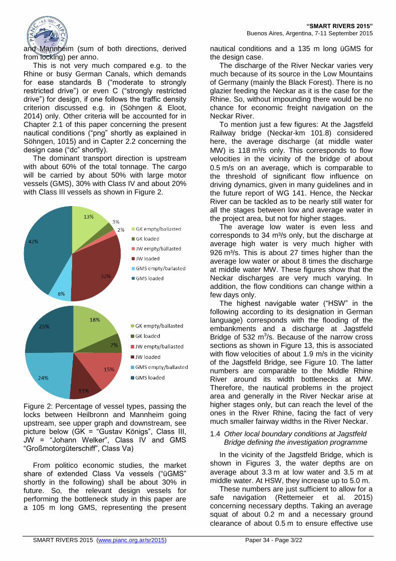
The dominant transport direction is upstream with about 60% of the total tonnage. The cargo will be carried by about 50% with large motor vessels (GMS), 30% with Class IV and about 20% with Class III vessels as shown in Figure 2.

Figure 2: Percentage of vessel types, passing the locks between Heilbronn and Mannheim going upstream, see upper graph and downstream, see picture below (GK = “Gustav Königs”, Class III, JW = “Johann Welker”, Class IV and GMS “Großmotorgüterschiff”, Class Va)

From politico economic studies, the market

share of extended Class Va vessels (“üGMS” shortly in the following) shall be about 30% in future. So, the relevant design vessels for performing the bottleneck study in this paper are a 105 m long GMS, representing the present

nautical conditions and a 135 m long üGMS for the design case.

The discharge of the River Neckar varies very much because of its source in the Low Mountains of Germany (mainly the Black Forest). There is no glazier feeding the Neckar as it is the case for the Rhine. So, without impounding there would be no chance for economic freight navigation on the Neckar River.

To mention just a few figures: At the Jagstfeld Railway bridge (Neckar-km 101.8) considered here, the average discharge (at middle water

MW) is 118m³/s only. This corresponds to flow velocities in the vicinity of the bridge of about

0.5m/s on an average, which is comparable to the threshold of significant flow influence on driving dynamics, given in many guidelines and in the future report of WG 141. Hence, the Neckar River can be tackled as to be nearly still water for all the stages between low and average water in the project area, but not for higher stages.

The average low water is even less and corresponds to 34 m³/s only, but the discharge at average high water is very much higher with

926m³/s. This is about 27 times higher than the average low water or about 8 times the discharge at middle water MW. These figures show that the Neckar discharges are very much varying. In addition, the flow conditions can change within a few days only.

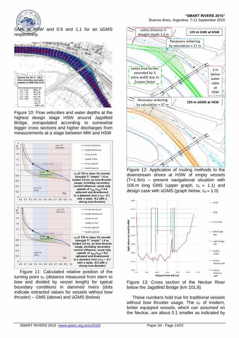
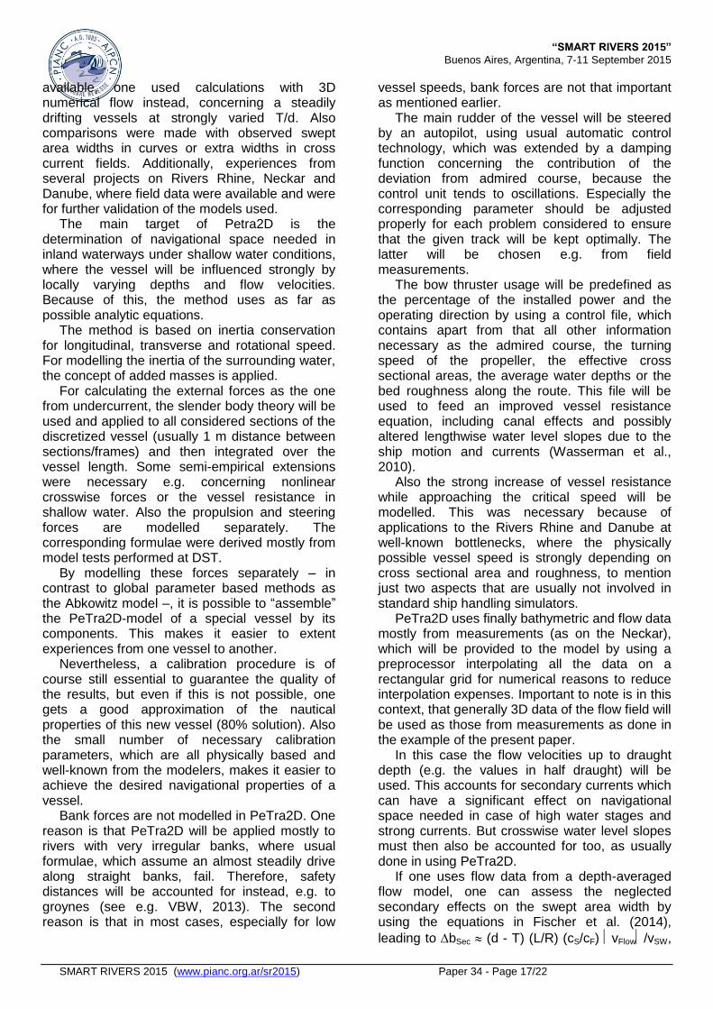
The highest navigable water (“HSW” in the following according to its designation in German language) corresponds with the flooding of the embankments and a discharge at Jagstfeld Bridge of 532 m3/s. Because of the narrow cross sections as shown in Figure 13, this is associated with flow velocities of about 1.9 m/s in the vicinity of the Jagstfeld Bridge, see Figure 10. The latter numbers are comparable to the Middle Rhine River around its width bottlenecks at MW. Therefore, the nautical problems in the project area and generally in the River Neckar arise at higher stages only, but can reach the level of the ones in the River Rhine, facing the fact of very much smaller fairway widths in the River Neckar.

1.4 Other local boundary conditions at Jagstfeld Bridge defining the investigation programme

In the vicinity of the Jagstfeld Bridge, which is shown in Figures 3, the water depths are on

average about 3.3m at low water and 3.5 m at middle water. At HSW, they increase up to 5.0 m.

These numbers are just sufficient to allow for a safe navigation (Rettemeier et al. 2015) concerning necessary depths. Taking an average squat of about 0.2 m and a necessary ground

clearance of about 0.5m to ensure effective use





of typical 4-canal bow thrusters, which suck water from below the vessel bottom, this leads to 2.7 m draught + 0.2 + 0.5 m = 3.4 m necessary depth, which is just between 3.3 and 3.5 m.

So, the nautical problems at the Jagstfeld Bridge do not arise from inadequate depth, but mostly from the available navigational widths below the bridge! The net width between the

foundations of the bridge piers is about 28m (24 m at the headroom) and is not very much more at higher stages (Figure 4)

Figure 3: Sketch from the waterway map (upper picture) and view from the vessel bridge (lower picture, field investigation of BAW in 2010 with an length-extended vessel according to Figure 8), sailing downstream just above the Jagstfeld Bridge at Neckar km 101.8

For comparison: This is not very much more

than the recommendations of WG 141 concerning the minimum width oft straight sections of one-lane canals, which are twice the vessel breadth B (Rettemeier 2015), giving 22.8 m. And this value has to be extended according to the recommendations by extra widths in curves, because the bridge is in a left turn with a radius R of the stream center line of about 1000 m at that place. Therefore, some extra width in curves should be added, which amounts to about 5.5 m if the Dutch guidelines will be applied (taking the parameters of an empty vessel and a vessel length L of 105 m).

This ends up with a necessary width of approximately 28 m and equals the existing width in draught depth, but not the width in the headroom. Therefore, a safe downstream drive at the Jagstfeld Bridge, especially for empty or container carrying vessels (2 layers), requires to

sail as straight as possible between the piers and make the left turn just after the bridge.

But this driving style leads to a smaller radius of the vessel course of about 300 m behind the bridge, as indicated by measurements shown in Figure 4. Hence, the nautical problem is to find out an optimal course to restrict extra widths in curves, together with choosing an optimal speed, ensuring both bow thruster and main rudder effectiveness. The first criterion demands for low vessel velocities relative to water, the second for high vessel speeds. Maybe both of two different ways of driving can solve the nautical problem or somewhat in between.

Apart from that one has to pay attention to the permitted vessel speed over ground of 16 km/h, and the vessel is limited by the critical speed too. This is due to the so-called canal-effects, which are present even at high stages, because the width in draught depth up- and downstream of the bridge is about 90 m only and therefore smaller than the vessel length and the blockage coefficient (vessel cross section, divided by effective channel cross section) of a fully laden vessel (T=2.7m) is about 0.09 at HSW and about 0.13 at MW, which is comparable to empty vessels in German standard canal sections (cross section at Jagstfeld Bridge see Figure 13). So, canal effects have to be accounted for, at least concerning the vessel resistance and the vessel speed, to find out the optimal way of driving.

It shall be mentioned additionally that driving situations at high stages can occur several times a year, even if the average probability of occurrence of HSW is small. This is because the water stage can generally change in a few days from low water up to the highest navigable water. In these cases the pilots try to “escape” as fast as possible towards the Rhine at a rising stage. Thus, the highest navigable water is definitively relevant for design.

This holds especially true in river sections just upstream of the next dam, because the stage, and therefore the navigable water depth, is nearly the same for HSW as for low water, but the discharge and the corresponding flow velocity will be very much higher. This holds true even in the project area at Jagstfeld Bridge, where the highest navigable stage is about 1.7 m higher than at low water (hydrostatic stage) or about

1.5m more than at MW, because the extra width needed to make the sharp left turn below the bridge can be bigger than the extra available navigational space due to the 1:3 sloped banks

(extra available space to the outer bend 1.53

5m) at higher stages. Thus, both the average water stage – because of less available space –





and HSW – because of bigger swept area width – have to be considered in the following.

Figure 4: Ship positions of 8 GMS (4 downstream, 4 upstream, 4 partially loaded with 1.6 - 1.9 m, 4 fully loaded with 2.7 m, 4 times mass cargo vessel “Hanna Krieger”, 4 times container carrying “Excelsior”, light green colored sailing downstream, dark green upstream) at stages around MW in the project area at Jagstfeld Bridge (Neckar km 101.8), derived from long-time vessel observations using stationary mounted GPS compasses

Further, since the extra width of a drifting

vessel in curves is heavily dependent on the draught to water depth ratio T/d, with higher values in case of an empty or ballasted vessel as shown e.g. in Figure 11, it was secondly not clear at the beginning of this navigational study, whether an empty vessel, which needs more space while drifting in curves if no or weak bow thrusters are available, but has got more space in draught depth than a fully loaded vessel, will have

more problems than a loaded vessel (T 2.7 m). Hence, both an empty and a ballasted vessel (assuming an average draught T of about 1.6 m) will be considered in the following.

But because a downstream drive is very much more risky because of the potential damages and the wider swept areas, which can be seen in

Figure4, where some results of field investigations concerning modern GMS around the Jagstfeld Bridge are collected, downstream drives will be considered here only, not upstream drives. This holds true also for windy conditions, because the additional width due to strong wind in an inland stretch, which is about 5% of the vessel length L according to Dutch Guidelines and WG 141 recommendations, is nearly the same sailing downstream or upstream. And because its influence on fairway design thus is minor if one

compares the existing with the future conditions, leading to 5% of the difference of the corresponding vessel lengths of 30 m, giving

1.5m only, there is no need to consider wind influences in the present study, if one extends the possible fairway widening by the a.m. value. Finally, because meetings may be possible, even just below the bridge, if both bridge openings will be used, but will be avoided in practice, only one-lane traffic will be regarded.

It should be added that poor visibility conditions are indeed important at the Jagstfeld Bridge, resulting in a bigger necessary navigational space, but the visibility conditions are presently and in future about the same. So, if one performs comparative considerations with the main objective to determine a necessary fairway widening, special attention to poor visibility conditions is not necessary.

1.5 Further nautical conditions

The majority of the vessels sailing on the Neckar River belong to a few shipping companies. Most of the skippers come from families that sail since decades on the Neckar River. Together with the fact that the transport relations are on an average short compared e.g. to the one on the Rivers Rhine or Danube, the route knowledge and the skills of the helmsman sailing on the Neckar River are nearly optimal. This is one reason why fast time simulations, which use track-keeping algorithms, may be adequate for performing a detailed navigational study in the reach considered, because these algorithms steer the vessels nearly optimally, as well as a very experienced driver will do. Nevertheless, it makes sense to account for human-factor effects additionally, e.g. using empirical formulae, see more in Chapter 3.4.

But even the best knowledge does not overcome the problems of driving dynamics in a quickly flowing river with narrow bends as in the project area considered at HSW. These can be solved by good equipped vessels only.

This can be assumed for üGMS as market analyses of existing extended GMS, performed by ANH, show. Taking the time for improvement of the Neckar locks, one came up with the following properties of the design vessel:

Length 135 m, breadth 11.45 m according to lock dimensions

2 wheels because of admission requirements (Rhine tributaries), Kort Nozzles, twin rudders

Propeller Diameter 1.6 m

Total installed main power 1600 kW





Rotational speed 350 rpm

4-channel bow thruster with an installed

power 600 kW The last mentioned value is the most important

one, because the loss of efficiency of this very strong bow thruster due to vessel velocity relative to water is minor compared to the very much weaker bow thrusters of the existing Neckar fleet.

The definition of adequate properties of the reference vessel of the existing fleet is more complicated and very much more far-reaching. If one uses e.g. the typically very much weaker bow thrusters for the reference vessel of the a.m. MS Hanna Krieger with 205 kW or the one of the MS Excelsior with 295 kW, the effectiveness of these bow thrusters may be strongly reduced at usual vessel speeds.

This can be checked using the observations shown in Figure 4 at stages around MW. The speed relative to water equals to 2.4 m/s, concerning the mostly fully loaded bulk cargo carrying MS Hanna Krieger (T=2.7 m) and about 3.3 m/s concerning the container vessel Excelsior

(T = 1.6 - 1.9 m, average 1.7 m). According to scale model tests at DST (report

1889, 2008), these vessel velocities lead to minor crosswise bow thruster forces, especially for the one of MS Hanna Krieger. This means that there may be no significant reduction of the simulated navigational space due to bow thruster usage in case of traditional shipping in the Jagstfeld Bridge section for this vessel, ending up in a big swept area width for the reference case, the existing situation in the present example.

This, in turn, may lead to a faulty decision concerning e.g. the necessary widening of the fairway, in case if the longer, but very much better equipped üGMS. These vessels may be able to sail more “slender” just at the bridge opening because of its effective bow thrusters compared to the existing vessels The corresponding difference in swept area width needed between reference and design case may then be small, which defines the necessary widening.

In contrast, if one uses stronger powered bow thrusters for the reference case, here the present nautical condition (“png” shortly in the following), which holds true for very new GMS, the difference between space needed between “png” and “dc” will be bigger than for the weaker powered reference vessel and so, the necessary widening.

This obviously surprising result of a navigational study, meaning that better equipped existing vessels may lead to a possibly over designed fairway for bigger vessels, can be overcome if the corresponding ease of navigation will be accounted for. If thus stronger bow

thrusters will be used in the reference case, this means that the corresponding ease quality is low. If this quality may be acceptable for design, this, in turn, would lead to the demand of the same low ease quality for design too, meaning that the üGMS have to take all their navigational means and thus, sail with reduced navigational space, leading to a smaller necessary widening.

On the other hand, if weaker thrusters will be assumed as the one of the a.m. MS Hanna Krieger, which act not effectively and so, it makes no sense to use it, it is more easy to steer the vessel in the present situation, which demands for the same easiness in design, leading to e.g. a reduced percentage of bow thruster power, and so, to an extended navigational width needed.

This means in particular that it may be necessary to choose the ease reference case (“erc” shortly), which is defined and used in Söhngen (2015) to compare simulation results quantitatively, e.g. the navigational space needed between “dc” and “erc”, differently to “png”, if the latter is using the better equipped vessels of the existing fleet as the MS Excelsior. Therefore, a proper choice of “erc”, which can be made using the “simplified s&e approach” approach according to Figure 5 in Chapter 2.1 (see for details Söhngen & Eloot, 2014 and Söhngen, 2015) is necessary, including an adequate choice of the bow thruster power, here the one of the MS Hanna Krieger, which is typical for the Neckar fleet and ensures that its effect is minor at Jagstfeld railway bridge.

All the chosen properties of this reference vessel are given in the following:

Length 105 m, breadth 11.4 m

1 wheel, Kort nozzle, twin rudders

Total installed main power 950 kW

Rotational speed 335 rpm

Propeller Diameter 1.7 m

4-channel bow thruster, 205 kW

2. RECOMMENDED DESIGN STEPS

The numbers of the following subchapters are identical to the numbering in Figure 3 of Söhngen (2015). Because of its importance, the application of the three recommended design methods: Concept Design, Practice Approach and Case by Case Design, according to step (6) in Figure 3 of the last mentioned paper and the corresponding paragraph 2.6 as well as step (7), will be treated additionally and in more detail in separate Chapters 3 (Concept Design), 4 (Practice Method) and 5 (Detailed Design) of this paper.

Therefore, the results from Chapters 3 to 5 have to be used in the subchapters 2.6 up to 2.8





to finish all the recommended design steps. These results will be used finally in Chapter 6 to develop a proposal for possible fairway widening.

2.1 Analyse the present nautical conditions

In the following the s&e quality of “png” will be analyzed, using the simplified approach outlined in Söhngen (2015). This first step is important in the present example especially because of two reasons: (1) The existing nautical conditions are generally

accepted by skippers and waterway authorities, even for the worst conditions with the largest permitted vessels and water stages. Therefore, the nautical conditions at “dc” will be accepted if they will not getting worse in future. Hence, the easy quality of “png” can thus be an image of the strived quality for “dc”, see chapter 2.2.

(2) Additionally “png” can then be used as the ease reference case, see Chapter 5.6, if the present boundary conditions are close to the ones at design. Here, they are almost identical.

(3) There are generally data of good quality available for “png”, which can be used to verify the simulation models (“verification reference case” or “vrc” shortly) for boundary conditions compared to “dc”, see Chapter 5.4. For this reason the ease score of “vrc” should be comparable to “dc” too. The principles of the simplified approach are

outlined e.g. in (Deplaix & Söhngen, 2013 and Söhngen & Eloot, 2014). They use several criteria, which speak for a higher or a lower existing ease quality according to three categories with the following designations:

(A) “Nearly unrestricted drive”, (B) “Moderate to strongly restricted drive” and (C) “Strongly restricted drive” The review of the published approach led to

the procedure in Figure 5, concerning the analysis of a present nautical condition and Figure 6 for assessing the necessary ease quality for design. New compared to the a.m. papers is that the applier of the approach is forced to assign scores according to the validity of each argument.

Figure 5: WG 141 proposal for assessing the ease quality of a driving situation under consideration, here the present nautical conditions with 105 m long GMS at Jagstfeld Bridge for stages between MW and HSW

If for example the 2nd, green-colored argument of the waterway related criteria in Figure 5 (criterion 2) is true, meaning that the helmsman are optimally qualified and experienced, which can be assumed in our example, one has to assign the highest score of +1, which speaks for a high existing ease score, as it was done in Figure 5. If

on the opposite, the corresponding red-colored argument holds true, one has to assign the lowest ease score of -1. So the scores are between +1 and -1, which can be assigned to the ease designations A and C respectively. Accordingly, all the other criteria were tackled in Figure 5.





To match all the scores one has to multiply them with a “single factor” first, which is chosen to sum up to unity for each of three criteria groups, which are related to waterway, vessel and traffic properties. This gives three comprehensive scores, which will then be weighed again by the “group factor”, which amounts again to unity. In effect, one receives a comprehensive score between +1 and -1, reflecting the corresponding assignations A and C.

Because the approach speaks for itself and all the data and arguments necessary can be found in the previous Chapter 2, Figure 5 will not be commented further. The result for the present nautical conditions, having especially the a.m. vessels Hanna Krieger and Excelsior in mind, is a score between 0 and +1, which is assigned graphically to the a.m. designations in Figure 7.

According to the expectations, the ease quality is between A and B, even in the vicinity of the Jagstfeld Bridge. This is especially due to well-equipped vessels, experienced helmsman and generally a sufficient speed range between critical

speed and minimum speed of about 5km/h at usual stages, which can be seen from the

widespread of observed vessel velocities and the small traffic density, together with very low recreational traffic density.

So, navigation on the River Neckar is clearly not as easy as e.g. on the Rhine, apart from the well-known bottlenecks, but still not as tricky as e.g. on the German River Danube in its free flowing section between Straubing and Vilshofen. This is because the River Neckar is an impounded river with high, but not extremely high flow velocities and generally regular shorelines. And the moderate number of accidents speaks for the same ease ranking. So, one can accept the results of assessing the ease score of “png”.

2.2 Choice of necessary s&e quality for design

An analogous approach concerning the design case is shown in Figure 6. It concerns to the necessary ease score, not the existing one. Because of this, e.g. the a.m. criterion of optimally qualified and experienced helmsmen is an argument that a lower ease score may be acceptable, see Figure 6 for details.

Figure 6: WG 141 proposal for assessing the necessary ease quality for design, here concerning the drive of üGMS at Jagstfeld Bridge for stages between MW and HSW

The chosen scores marked with an asterisk,

differ from corresponding values in Figure 5. The first concerns to the pilots skills. In contrast to the existing situation, one has to assume that extended Class Va vessels will generally sail on

the River Rhine and seldom on the Neckar. So, the route knowledge will not be as good as nowadays, demanding for a higher necessary score, see criterion 2 in Figure 6. Also the exploitation of existing fairway widths is greater





for üGMS in curves, demanding for more ease quality (criterion 4). On the other hand, one can assume that the üGMS are very much more powered and better steerable than the vessels of “png”, leading to a lower necessary ease score, see criterion 7. Finally, the hindrance due to recreational boating will probably increase in future, leading to a higher necessary ease score as nowadays.

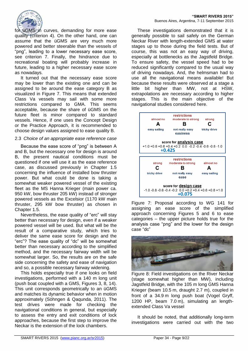
It turned out that the necessary ease score may be lower than the existing one and can be assigned to be around the ease category B as visualized in Figure 7. This means that extended Class Va vessels may sail with some more restrictions compared to GMA. This seems acceptable, because the share of üGMS on the future fleet is minor compared to standard vessels. Hence, if one uses the Concept Design or the Practice Approach, it is recommended to choose design values assigned to ease quality B.

2.3 Choice of an appropriate ease reference case

Because the ease score of “png” is between A and B, but the necessary one for design is around B, the present nautical conditions must be questioned if one will use it as the ease reference case, as discussed previously in Chapter 1.5 concerning the influence of installed bow thruster power. But what could be done is taking a somewhat weaker powered vessel of the existing fleet as the MS Hanna Krieger (main power ca. 950 kW, bow thruster 205 kW) instead of stronger powered vessels as the Excelsior (1170 kW main thruster, 295 kW bow thruster) as chosen in Chapter 1.5.

Nevertheless, the ease quality of “erc” will stay better than necessary for design, even if a weaker powered vessel will be used. But what will be the result of a comparative study, which tries to deliver the same ease score for design and the “erc”? The ease quality of “dc” will be somewhat better than necessary according to the simplified method, and the necessary fairway width will be somewhat larger. So, the results are on the safe side concerning the safety and ease of navigation and so, a possible necessary fairway widening.

This holds especially true if one looks on field investigations, performed with a 140 m long unit (push boat coupled with a GMS, Figures 3, 8, 14). This unit corresponds geometrically to an üGMS and matches its dynamic behavior when in motion approximately (Söhngen & Qaqunda, 2011). The test drives were made for checking the navigational conditions in general, but especially to assess the entry and exit conditions of lock approaches, because the first step to improve the Neckar is the extension of the lock chambers.

These investigations demonstrated that it is generally possible to sail safely on the German Neckar River with length-extended GMS at water stages up to those during the field tests. But of course, this was not an easy way of driving, especially at bottlenecks as the Jagstfeld Bridge. To ensure safety, the vessel speed had to be reduced significantly compared to the usual way of driving nowadays. And, the helmsman had to use all the navigational means available! But because these results were observed at a stage a little bit higher than MW, not at HSW, extrapolations are necessary according to higher stages. This is the main objective of the navigational studies considered here.

Figure 7: Proposal according to WG 141 for assigning an ease score of the simplified approach concerning Figures 5 and 6 to ease categories – the upper picture holds true for the analysis case “png” and the lower for the design case “dc”

Figure 8: Field investigations on the River Neckar (stage somewhat higher than MW), including Jagstfeld Bridge, with the 105 m long GMS Hanna

Krieger (beam 10.5m, draught 2.7 m), coupled in

front of a 34.9m long push boat (Vogel Gryff,

1200 HP, beam 7.0m), simulating an length-extended Class Va vessel

It should be noted, that additionally long-term

investigations were carried out with the two





vessels shown in Figure 4, providing information on usual vessel courses, swept area widths and vessel speeds at all design relevant stages, especially those close to the highest navigable water level. These data were used not only for nautical purposes, but also for assessing the bed and bank impact, especially to account for environmental demands as avoiding an increased turbidity or wave loads on ecologic sensitive bank areas.

But the measured swept area widths can be used additionally, together with the ones of our artificially extended unit, to assess the necessary fairway width for all relevant stages as HSW. This will be done from BAW using the observed navigational widths, plus the differences between all the relevant additional widths at design situation and observations. These are the extra widths in curves, in cross flow fields or according to the human factor. Because these differences are generally very much smaller than the absolute values, they can be calculated with sufficient accuracy with semi-empirical formulae, which will be published in the future report of WG 141 (see e.g. Söhngen, Feierfeil & Paprocki, 2014 for applications on the Rhine). Only safety distances have to be accounted for directly, but they are also an order of magnitude smaller than the other parts of the necessary fairway width. But because this approach works for almost steadily driving conditions only, not for manoeuvring situations as bridge passages, they will not be applied in the following.

2.4 Check the sensitivity of ease scores

The weighting factors in Figures 5 and 6 are still under discussion in WG 141 and should thus be understood as a first attempt. On the other hand, they are “not cast in stone” and should be modified e.g. if the results do obviously do not match with experiences or if the same approach, but with other weighting factors, was chosen for another project, in order to be able to compare results. But our results obviously fit with experiences and thus support the chosen factors. This holds true even if the weighting factors will be modified. This means that the evaluated ease categories are not very sensitive to the chosen weighting factors. So, the results can be accepted.

2.5 Specify the strived ease standards

As argued before, the strived ease standards for design should be at least category B or better. Because of unavoidable modelling inaccuracies in using simulation techniques, the standard of “erc”

should be about the same as in “pnc”, which is somewhat better than B as explained earlyer.

2.6 Perform the design, using all the 3 methods

With reference to the following chapters, one ends up concerning the main objective of the study, a possibly necessary channel widening, with three totally different results:

The application of the Concept Design Method according to Chapter 3.4 leads to 22.5 m more space needed.

The Practice Approach defines a necessary widening of about 10.5 m, sere Chapter 4.2.

Chapter 5.9 deals with the results of fast time simulations, leading to at least 2.5 m up to about 12.5 m more navigational space. These results will be discussed concerning

possible recommendations to the planner of the Neckar improvement in Chapter 6.

2.7 Analyse the ease quality in applying the Detailed Design

Besides the usual way to use results of simulation techniques, especially those from ship handling simulators, as talking with the skippers in the sense of an expert rating, which is very important anyway, WG 141 proposes additionally a rational approach similar to the simplified one outlined in Chapters 2.1 and 2.2, defining an index-system analogous to the ease score. This approach is essential in case of using fast time simulations as in our example, simply because there are no real pilots available to be consulted.

Because the decision about the necessary ease standard for design and the corresponding ease reference case must be taken before applying simulation techniques and because the design case has to be specified also in advance (and all the relevant boundary conditions), e.g. using the Concept Design Method, the following approach is made to analyze simulation results only, not to define necessary indexes. The approach is then comparable with the analysis case in Figure 5 only, but both “dc” and “erc” will be analyzed.

In order to do this, one has to decide first, whether the indexes should reflect the “easiness” and “safety” of a driving situation, leading to high index values for an easy drive and low values for a complicated or unsafe condition, or if the “difficulty” of a manoeuvring condition should be assigned with appropriate indexes. The higher the difficulty, the higher is the corresponding index.

Users of Ship Handling Simulators often use indexes related to the difficulty. This has the advantage that the index can be made open upwardly as the Richter-scale concerning the





strength of earthquakes. Alternatively and analogous to the ease scores in Figures 5 and 6, we will use here index values or ease scores, if we will call it alternatively by analogy with the simplified approach, taken between -1, which may be related to ease quality C, 0, corresponding to B and +1, which is related to ease quality A, see also Figure 9. But it should be noted that the corresponding concrete figures will not be the same than those from the simplified approach. So, only differences of these scores between “erc” and “dc” should be uses for decisions about the ease category achieved. Nevertheless, with an appropriate choice of the parameters to define the a.m. indexes, it may possible to end up with scores which are directly comparable to the ease categories between A and C.

Analogous to different rating groups of the simplified approach, the ease of a driving situation may be assessed by collecting different values from simulation runs as rudder angles into rating groups again. For this we use the following table, defining two groups: The first is called “exploitation of resources” and the second “driving difficulty and handicaps”. The chosen subgroups refer to mainly waterway related aspects and its special boundary conditions, to the properties of the vessels and the influence of the helmsman, see Table 1 for details.

Group Sub-group

Characteristic value from simulations

Explo

ita

tion o

f

resourc

es W

ate

r-

way

rela

ted

Percentage of permitted speed

Percentage of vcrit

Bank distance

Swept area width

Vessel

rela

ted

Main rudder angle

Percentage of bow thruster power used

Percentage of main power usage

Drivin

g d

ifficu

lty

and h

an

dic

aps

Hum

an

rela

ted

Number of rudder actions (incl. bow thruster) per minute

Standard deviation of swept area width

Vessel

rela

ted

Standard deviation of rpm

Standard deviation of main rudder angles

Rudder angular velocity

Table 1: Rating groups with selected characteristic values from simulations for assessing an ease index (chosen values for Jagstfeld study in bold print)

But it seems not necessary to account for all the characteristic values in Table 1 for the present example, because the fast time simulations runs for the present example work generally with some predefined values as the mostly constant rotation

speed of the main propeller or the bow thruster usage, whereby for simplification always 100% of the installed power will be taken as usual in practice at bottlenecks. So, the criteria related to power used will not be significantly different in “dc” and “erc” and can thus be neglected. This holds true for the vessel speed criteria too, since the vessels sail far below the critical speed and because it is usual practice to exploit the permitted vessel speed of 16 km/h if possible. So, we choose the following values from simulations for making the comparisons, see Table 2.

Exploitation

Waterway related

Bank distance 0.3

Vessel related Main rudder angle 0.2

Bow thruster usage 0.2

Difficulty

Human related Number of rudder actions (incl. bow thruster) per minute 0.15

Vessel related Standard deviation main rudder angles 0.15

Table 2: Selected characteristic values from Table 1 to compare “dc” with “erc” with corresponding weighting factors (blue-colored) for matching the different s&e indexes

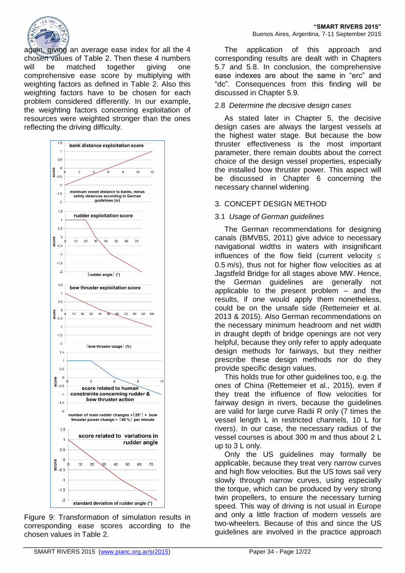
The assignation of the values in Table 2 to corresponding ease scores is shown in Figure 9. It follows the principle that a score of +1, which corresponds to ease category A, was assigned to “usual values” as one vessel breadth concerning the bank distance, 20° concerning the rudder angle and the corresponding standard deviation as well as 3 rudder actions per minute, which refers to the average reaction time of helmsman steering sea-going vessels according to investigations of Ji Lan et al. (2000). On the opposite, ease scores of -1 will be assigned if e.g. 45° rudder angle will be overtopped, because even higher numbers do not improve the rudder effectiveness according to the crosswise force anymore as model tests of DST for typical twin rudders of modern GMS show. So, this score can be related to ease category C. But it must be clear that all these numbers have to be adjusted to the special design problem considered.

This transformation of values from simulations to corresponding scores will now be applied to each value of the corresponding time series and then averaged over the critical river section between Neckar-km 108.7 (100 m upstream of the bridge) and 108.4, where the vessels sail nearly undisturbed from the bridge passage





again, giving an average ease index for all the 4 chosen values of Table 2. Then these 4 numbers will be matched together giving one comprehensive ease score by multiplying with weighting factors as defined in Table 2. Also this weighting factors have to be chosen for each problem considered differently. In our example, the weighting factors concerning exploitation of resources were weighted stronger than the ones reflecting the driving difficulty.

Figure 9: Transformation of simulation results in corresponding ease scores according to the chosen values in Table 2.

The application of this approach and corresponding results are dealt with in Chapters 5.7 and 5.8. In conclusion, the comprehensive ease indexes are about the same in “erc” and “dc”. Consequences from this finding will be discussed in Chapter 5.9.

2.8 Determine the decisive design cases

As stated later in Chapter 5, the decisive design cases are always the largest vessels at the highest water stage. But because the bow thruster effectiveness is the most important parameter, there remain doubts about the correct choice of the design vessel properties, especially the installed bow thruster power. This aspect will be discussed in Chapter 6 concerning the necessary channel widening.

3. CONCEPT DESIGN METHOD

3.1 Usage of German guidelines

The German recommendations for designing canals (BMVBS, 2011) give advice to necessary navigational widths in waters with insignificant

influences of the flow field (current velocity

0.5m/s), thus not for higher flow velocities as at Jagstfeld Bridge for all stages above MW. Hence, the German guidelines are generally not applicable to the present problem – and the results, if one would apply them nonetheless, could be on the unsafe side (Rettemeier et al. 2013 & 2015). Also German recommendations on the necessary minimum headroom and net width in draught depth of bridge openings are not very helpful, because they only refer to apply adequate design methods for fairways, but they neither prescribe these design methods nor do they provide specific design values.

This holds true for other guidelines too, e.g. the ones of China (Rettemeier et al., 2015), even if they treat the influence of flow velocities for fairway design in rivers, because the guidelines are valid for large curve Radii R only (7 times the vessel length L in restricted channels, 10 L for rivers). In our case, the necessary radius of the vessel courses is about 300 m and thus about 2 L up to 3 L only.

Only the US guidelines may formally be applicable, because they treat very narrow curves and high flow velocities. But the US tows sail very slowly through narrow curves, using especially the torque, which can be produced by very strong twin propellers, to ensure the necessary turning speed. This way of driving is not usual in Europe and only a little fraction of modern vessels are two-wheelers. Because of this and since the US guidelines are involved in the practice approach





of WG 141 anyway (see Figure 2 in Söhngen, 2015), which will be applied in 4.1 of this paper, they will not be applied separately here.

Nevertheless, the recommended way to use routing methods for designing fairways and account for safety margins in German Guidelines can and will be used in the following, see Chapter 3.3, because this approach is generally not restricted to still water, if adequate relative positions of the turning point (cF-values) will be used. For definition of cF, corresponding design graphs and conditional equations see e.g. (Söhngen et al., 2013b, VBW, 2013 and Fischer et al., 2015) and Figures 11 and 12 in this paper.

3.2 Recommendations of WG 141

There are no specific recommendations of WG 141 available at the present state concerning the minimum net width of bridge openings in applying the Concept Design Method, but it is obvious that this width should be at least the recommended minimum width in draught depth of canals, which is 2·B, plus relevant increments as those in curves or wind. If one follows this rule, assuming a straight passage of the opening and taking the Dutch “rule of thumb” concerning wind influence (5 % of vessel length for an inland stretch), which is valid not only for empty vessels in our case, but also for container carrying vessels, because only 2 layers are possible on the River Neckar, which fit concerning the height over the water table well with empty vessels, one ends up with at least

28m necessary width in draught depth of an empty vessel. This number can be compared to the net bridge opening in draught depth, which is

approximately 34 m at higher stages ( MW), see bridge cross section in Figure 13, and the guaranteed width of the headroom which is about 24 m. This means that the existing width in draught depth may be sufficient according to this criterion, but not for the headroom.

So, even the lowest standards for fairways in canals cannot be fulfilled at Jagstfeld Bridge for all vessels. But because the available space is just acceptable concerning this rule if wind influence may be not important and the passage follows a straight course as assumed, one could mount crash barriers on both sides of the bridge opening to ensure a safe navigation by “body contact” if necessary. This is one of the possible recommendations to the planners of the Neckar improvement. Because of this, it will be accepted in the following that usual safety distances may not be kept, but one should make sure that the future situation with üGMS does not get worse.

If one looks in existing guidelines, one can find design rules from China, demanding for at least 2

B and from US to be at least 2.75 – 3.5 B. So, again 2 B seems to be a lower limit for a straight passage as assumed above.

Besides that, WG 141 recommends to perform detailed studies in case of significant flow influences on design, especially for manoeuvring conditions as at Jagstfeld Bridge. Nevertheless Concept Design and Practice Approach should be applied in every case additionally for comparisons.

Just upstream and downstream of the bridge opening the recommended design rules of WG 141 are the same as the ones for fairways in rivers. Taking the considerations above, there will be no differentiation between bridge opening and remaining river sections in the following.

3.3 Application of routing methods

Because there are no significant cross currents in the project area, routing methods seem applicable. As outlined e.g. in the German guidelines (BMVBS, 2011), one has to specify an appropriate vessel course first, here taking field data as shown in Figure 4 as a basis. After that, vessel symbols will be placed using CAD programs tangential to the route at the turning point in chosen intervals along the route. The envelope of the series of symbols forms the constructed swept area. This is shown in Figure 12 for the design-relevant boundary conditions.

The “art” of applying the routing method is to find out an optimal course, which delivers the narrowest swept area. In our example, we tried to sail as straight as possible through the bridge opening with regard to safety margins to bridge piers (4 m according to German guidelines) and embankments (1.5 m) up- and downstream of the bridge.

The most important parameter to be chosen before applying the method is the position of the turning point, which is depending on vessel type, the of draught to water depth ratio T/d, the driving direction and the relation of flow velocity to vessel speed relative to water vFlow/vSW. For this, one can use experiences about typical vessel speeds in

dammed rivers, leading to vFlow/vSW 0.4 (data see VBW, 2013), which will be supported by measurements at Jagstfeld Bride for design-relevant stages (see Chapter 1.5 concerning vSW and Figure 10 concerning flow velocities).

This is shown in Figure 11, concerning cF-values for GMS and üGMS. If one looks further on typical T/d in dammed rivers as indicated in Figure 11, which are about the same as at the Jagstfeld Bridge, the design-relevant cF are about 1.0 for a loaded and 1.2 for an empty/ballasted





GMS at HSW and 0.9 and 1.1 for an üGMS respectively.

Figure 10: Flow velocities and water depths at the highest design stage HSW around Jagstfeld Bridge, extrapolated according to somewhat bigger cross sections and higher discharges from measurements at a stage between MW and HSW

Figure 11: Calculated relative position of the

turning point cF (distance measured from stern to bow and divided by vessel length) for typical boundary conditions in dammed rivers (dots indicate extracted values for vessels without bow thruster) – GMS (above) and üGMS (below)

Figure 12: Application of routing methods to the downstream drives at HSW of empty vessels (T=1.6m) – present navigational situation with

105m long GMS (upper graph, cF 1.1) and

design case with üGMS (graph below, cF 1.0)

Figure 13: Cross section of the Neckar River below the Jagstfeld Bridge (km 101.8)

These numbers hold true for traditional vessels

without bow thruster usage. The cF of modern, better equipped vessels, which can assumed on the Neckar, are about 0.1 smaller as indicated by





field data collected and analyzed by BAW. These reduced values will be used in the following for applying the routing method.

It turns out that the smallest distances between swept area envelope, which was extended sideways by half the extra width due to instabilities of the vessel path (total 4.1 m according to German guidelines) to account for human related effects, occurred for the smallest draughts considered (T=1.6m) and at the highest stage (HSW). So, the empty/ballasted vessel at the highest stage considered is design relevant only in using routing methods – even though the additional available space in draught depth at the most critical point just downstream of the bridge, is about 5 m wider for HSW compared to MW and about 3 m wider for a ballasted vessel compared to a fully loaded one (following from 1:3 sloped banks). This means that the extra width due to bigger cF at higher stages and smaller draughts is more important than the bigger available space in draught depth.

These conditions are typical for the River Neckar and can be checked before using the routing method by applying the usual formula for

extra widths in curves: bc = ½ cF2 L2 / B, leading

to e.g. 7 m difference between an empty or ballasted 105 m long GMS, which is more than the 3 m extra navigational space available (using R = 300 m).

3.4 Results according to comparative analyses

The results of applying the routing method, shown in Figure 12 need some explanations:

(1) There is always an overlap between extended swept area envelope and the nautically usable channel boundaries in draught depth (narrowed by safety margins). For the GMS this amounts up to maximal 17m! This contradicts to experience showing the vessels are able to stay between embankments. This is due to the fact that the applier of the routing method tried to meet with the safety margins just between the bridge piers, leading to an increases navigational width downstream to make the necessary turn after the bridge. Even more important is that the routing method is not able to account for a transverse offset manoeuve, which is usual just after passing the bridge, using all the navigational means available. Therefore, routing methods may give results far on the safe side in case of manoeuvring conditions!

(2) But one can use the principle of comparative considerations where model inaccuracies eliminate to some extent, taking not the total value of overlapping the channel boundaries, but the difference between “dc” and

“pnc” only, to overcome the problems in using the

routing method to some extent. This leads to 20m necessary widening of the fairway for üGMS. This number should be enlarged by wind influences as mentioned earlier, which amounts up to an extra difference of 1.5 m. Finally one should account for an increased extra width due to instabilities or

human factor respectively bI. For this, one can use an approach in VBW (2013), which was derived from data of the US guidelines and which supports the a.m. number of 4.1 m according to German guidelines for canals, but gives higher

values e.g. for rivers and long tows: bI = 0.7 m + 0.8 d vFlow/vSW + 0.023 L vSaG / vSW (vSaW = vessel speed above ground). If one applies this formula again according to differences between “dc” and “png” and taking 0.4 for vFlow/vSW as for assessing the cF, one ends up with about 1.0 m more necessary space for the longer üGMS.

(3) According to investigations of BAW, the safety distances to banks are very much depending on vessel speed, draught and channel width. For narrow cross sections as those at Jagstfeld Bridge, moderate vessel speeds and empty/ballasted vessels, they are and generally smaller than the ones in German guidelines. Therefore, the latter were chosen here. Hence, because they are about the same in “dc” and “pnc”, there will be no extra with to account for concerning the necessary widening of the channel. This result is obvious, because the vessel cross sectional area is the same in “dc” and “pnc”, which is the most important scaling parameter for safety margins to bank slopes, if vessel speed and channel width are about the same.

Figure 14: Field investigations with a length-extended vessel (light green symbols) in comparison to 105 m long GMS as shown in Figure 4 at stages around MW





Summarizing, using the principle of comparative investigations, this results would lead to 22.5 m more (20 m from wider swept area,

1.5m from more wind influence and 1.0 from more human effects) space at the outer bank over about 150 m length. But is this really realistic, facing the results of field investigations with an extended GMS, discussed in Chapter 2.3 and shown in Figures 3 and 8, especially if one looks on Figure 14, showing the swept area width at Jagstfeld Bridge at MW, which does definitively not overlap the swept area of the existing fleet. Answers shall be given in the following two chapters.

4. PRACTICE APPROACH

4.1 Design diagramme

Söhngen (2015) provides a graph relating fairway widths in use to the extra widths in curves for one-lane traffic. He interprets the spread of data according to the existing ease of navigation, taking the upper bound of the green colored reach in this figure as to be ease category A and the lower bound to be C, one ends up with the following formula for assessing the necessary fairway width: bF = n B + ½ L2 / R, with n = 4 for ease category A, 3 for B and 2 for C.

Applied to “dc” with L = 135 m, B = 11.45 m and R = 300 m, assuming category B, this gives 65 m necessary fairway width or about 32 m to the left and right hand side of the river axis, which is about the same as the existing space in draught depth. In opposite to the routing method, this would speak for no necessary widening of the channel.

But as stated already concerning the routing method, the special manoeuvring conditions will not be tackled by this very simple formulae, which seems thus to be applicable in river sections with slowly changing boundary conditions only. So, the Practice Approach fails if it will be used directly for design.

4.2 Application using comparative analyses

But one can apply the formulae comparatively again as follows: Taking the ease score difference of -0.35 between “dc” and “pnc” according to Figure 7, this leads to a lower necessary space

according to the ease category of 0.35 B = 4m. But because of the longer vessels, there is still a need of ½ (1352 - 1052) / 300 = 12 m wider

fairways, giving in total 8m necessary widening, if one assumes that the existing nautical conditions are just O.K.. Because of bigger increments due to human-related aspects and bigger wind

influences, this number should be extended to 10.5 m in total.

Compared to the result from the routing method of about 22.5 m, this is only 47 % of it. This shows that Concept Design and Practice Approach cannot solve the design problem considered. But the a.m. numbers give at least an idea on the order of magnitude of a possibly necessary channel widening

5. CASE BY CASE STUDY WITH TRACK KEEPING AND FAST TIME SIMULATION

Also this chapter follows the recommended design steps of WG 141. They are outlined in detail in Figure 4 of Söhngen (2015). With reference to this paper and for simplification, the numbering of the following subchapter is the same as the steps in this figure.

5.1 Data used and relevant boundary conditions

Because bow thruster usage seems to be a kernel aspect in sailing through the Jagstfeld bridge opening as stated earlier, especially because of the very much stronger bow thrusters of modern üGMS, and because this effect could be accounted for by using the a.m. simplified methods, the question is still open, which boundary conditions are relevant for design: WM with its smaller available widths or HSW with greater swept area widths? Deep draught vessels with longer reaction times and smaller available widths, but less space needed in curves in case of ineffective bow thrusters, or empty vessels because of a possibly wider swept area, even if a little bit more space is available toward the banks?

With reference to Chapters 1.3, 1.4 and 1.5, where all the other relevant boundary conditions were checked, e.g. that it seems not necessary to account for wind influences in a comparative study or referring to Chapter 3.4 concerning safety distances, the relevant boundary conditions are specified for the problem considered.

5.2 Simulation programme PeTra2D

In Figure 4 of Söhngen (2015) the next step is to check the modelling capacity of the simulation tool used. It is assumed here that this important step was performed with satisfactory results previously. Concerning the fast time simulation software PeTra2D, developed from Kolarov (2008) and extended by BAW (see also Linke, 2015), which will be used here, this calibration step was performed e.g. by comparing calculated and measured forces on the underwater body of the vessel. If there were no measurements





available, one used calculations with 3D numerical flow instead, concerning a steadily drifting vessels at strongly varied T/d. Also comparisons were made with observed swept area widths in curves or extra widths in cross current fields. Additionally, experiences from several projects on Rivers Rhine, Neckar and Danube, where field data were available and were for further validation of the models used.

The main target of Petra2D is the determination of navigational space needed in inland waterways under shallow water conditions, where the vessel will be influenced strongly by locally varying depths and flow velocities. Because of this, the method uses as far as possible analytic equations.

The method is based on inertia conservation for longitudinal, transverse and rotational speed. For modelling the inertia of the surrounding water, the concept of added masses is applied.

For calculating the external forces as the one from undercurrent, the slender body theory will be used and applied to all considered sections of the discretized vessel (usually 1 m distance between sections/frames) and then integrated over the vessel length. Some semi-empirical extensions were necessary e.g. concerning nonlinear crosswise forces or the vessel resistance in shallow water. Also the propulsion and steering forces are modelled separately. The corresponding formulae were derived mostly from model tests performed at DST.

By modelling these forces separately – in contrast to global parameter based methods as the Abkowitz model –, it is possible to “assemble” the PeTra2D-model of a special vessel by its components. This makes it easier to extent experiences from one vessel to another.

Nevertheless, a calibration procedure is of course still essential to guarantee the quality of the results, but even if this is not possible, one gets a good approximation of the nautical properties of this new vessel (80% solution). Also the small number of necessary calibration parameters, which are all physically based and well-known from the modelers, makes it easier to achieve the desired navigational properties of a vessel.

Bank forces are not modelled in PeTra2D. One reason is that PeTra2D will be applied mostly to rivers with very irregular banks, where usual formulae, which assume an almost steadily drive along straight banks, fail. Therefore, safety distances will be accounted for instead, e.g. to groynes (see e.g. VBW, 2013). The second reason is that in most cases, especially for low

vessel speeds, bank forces are not that important as mentioned earlier.

The main rudder of the vessel will be steered by an autopilot, using usual automatic control technology, which was extended by a damping function concerning the contribution of the deviation from admired course, because the control unit tends to oscillations. Especially the corresponding parameter should be adjusted properly for each problem considered to ensure that the given track will be kept optimally. The latter will be chosen e.g. from field measurements.

The bow thruster usage will be predefined as the percentage of the installed power and the operating direction by using a control file, which contains apart from that all other information necessary as the admired course, the turning speed of the propeller, the effective cross sectional areas, the average water depths or the bed roughness along the route. This file will be used to feed an improved vessel resistance equation, including canal effects and possibly altered lengthwise water level slopes due to the ship motion and currents (Wasserman et al., 2010).

Also the strong increase of vessel resistance while approaching the critical speed will be modelled. This was necessary because of applications to the Rivers Rhine and Danube at well-known bottlenecks, where the physically possible vessel speed is strongly depending on cross sectional area and roughness, to mention just two aspects that are usually not involved in standard ship handling simulators.

PeTra2D uses finally bathymetric and flow data mostly from measurements (as on the Neckar), which will be provided to the model by using a preprocessor interpolating all the data on a rectangular grid for numerical reasons to reduce interpolation expenses. Important to note is in this context, that generally 3D data of the flow field will be used as those from measurements as done in the example of the present paper.

In this case the flow velocities up to draught depth (e.g. the values in half draught) will be used. This accounts for secondary currents which can have a significant effect on navigational space needed in case of high water stages and strong currents. But crosswise water level slopes must then also be accounted for too, as usually done in using PeTra2D.

If one uses flow data from a depth-averaged flow model, one can assess the neglected secondary effects on the swept area width by using the equations in Fischer et al. (2014),

leading to bSec (d - T) (L/R) (cS/cF) vFlow/vSW,





with bSec = neglected width increment and cS 5.9, if no bow thruster will be used. In our example this would amount up to be about 7 m at HSW (T = 1.6, üGMS, cF = 1.0, vFlow = 1.9 m/s,

d=5.0 m). But, as mentioned before, this effect is included in our calculations directly because of interpreted field data used.

PeTra2D is running on standard desktop computers and is written in JAVA. Results of the computations are amongst others the ship trajectory, the swept path, the vessel speed over ground and relative to water, the critical ship speed, the rudder angles and all the forces, e.g. those from bow thruster usage, including its reduction at higher vessel velocities.

The vessel in PeTra2D can be steered not only by an autopilot, but also using optimization procedures, but concerning the main rudder usage only at the present stage of development. For this, all the rudder angles along the route will be predefined in a 1st step. Then the resistance file including these information will successively adapted using e.g. evolutionary strategies (Maaß, 2011). A somewhat simpler but very much faster and thus real-time capable algorithm will be used in the reengineered version of PeTra2D, the program FARAO, see Linke et al. (2015).

5.3 Comparision with present nautical conditions

Using data from numerous field investigations as those mentioned in Chapter 1.4 and Figure 4, the usual vessel speed relative to water for fully loaded GMS is nearly constant to be about

2.4m/s. Empty or ballasted vessels sail in the project reach about 0.9 m/s faster. This would

lead to 4.3m/s over ground in case of HSW for a loaded and 5.2 m/s for an empty vessel. Because the latter number would be much bigger than the maximum permitted vessel speed of 16 km/h = 4.4 m/s, we used the permitted speed as an upper limit, even if we had, despite of our long-term investigations, no exact information on used vessel speeds at HSW from that reach (relative to water 9 km/h). This restriction of vessel speed is important, because bow thrusters are almost ineffective at high vessel speeds, and thus the swept area width can be restricted by sailing very fast only. Nevertheless, because of the generally disciplined way of driving, one can assume that the speed limit will be kept from the skippers.

But usual safety distances will definitively not kept just between the bridge piers, especially towards the left pier, as Figure 4 indicates. Obviously the risk to touch the left hand pier, where the observed net distances between the vessels and the left bridge pear are minimal, is very little, obviously because bank forces are not

that important and because the vessel tends to drift towards the outer bend away from the left pier anyway. So, the usual way of driving is sailing as nearby as acceptable to the left pier and staring the turn just upstream of the bridge to avoid a too sharp turn downstream of the bridge.

If one follows these rules for the fast time simulations in all situations considered, here loaded and ballasted vessels at MW and HSW and using the design vessel defined in Chapter 1.5, the simulated vessels are able to stay inside the channel boundaries (defined by the geometrically available space in dynamic draught, which is about static draught plus 0.3 m to account for squat), which was narrowed by adequate safety distances as used for routing methods for simplification, besides just one point at the left pier.

The most critical conditions arose at HSW, both for the deep draught and the ballasted vessels see Figure 15, showing the situation of the ballasted vessel at HSW. The smallest distances to the drivable boundaries just downstream of the bridge were about 6 m, if we neglect smaller numbers just below the bridge, because a high attention level may be presumed just at this point.

Figure 15: Results of fast time simulation with PeTra2D, using the properties of the ballasted (T = 1.6 m) MS Hanna Krieger, sailing with the maximal allowed vessel speed over ground of about 16 km/h (on average 2.4 m/s relative to water), taking 180 rpm of the main engine

But because automatically steered vessels

were used in our fast time simulations, the a.m.

6m available space to the boundaries may be used up by human effects. If one applies for this purpose the formula for the corresponding additional width in Chapter 3.4, one ends up with about 9 m additional necessary space. If one takes half of this value concerning a possible sideways displacement towards the right bend (4.5 m) and correspondingly the half of the wind increment of about 0.05 L, giving about 2.5 m,





one ends up with additional 7 m. This is 1 m more than the existing net distance.

This means that, if the vessels would be steered by real, not virtual pilots as in PeTra2D, the available space is just sufficient upstream and downstream of the bridge, but not between the bridge piers. This means in particular for the comparative considerations that, if the extended Class Va vessels need significantly more space, this defines the necessary widening of the channel, taking additionally 2.5 m for different human and wind effects as mentioned before.

It should be noted that the simulation results are mainly depending on the vessel speed. It is really necessary to sail as fast as permitted in order to stay between the banks, as it is obviously practice. Nevertheless, there is still an option to sail very slowly, especially if the vessel is equipped with a 4-channel bow thruster, because one can use it both as a break and a bow rudder, which allows for to sustain main rudder force even at low vessel speeds. But this way of driving is definitively not easy at all.

5.4 Choice of a verification reference case “vrc”

To verify the modeling capacity, a well-known driving situation, which is close to the design case, should be used. For this reason, one could use the driving test with the unit according to Figure 14. But besides the fact, that it would be very complicated to model all the steering aids of this very special unit, this was definitively not a normal driving situation, especially because the helmsman of the push boat Vogel Gryff had no route knowledge before the tests. Therefore, he kept a bigger distance to the left pier, because in the reach he is usually sailing, there are generally gravel deposits towards the inner bank, also at bridge piers. So, the ship path was not optimal and the vessel speed was very low. Additionally, the bow thruster power of the unit used was very much lower compared to a modern üGMS. Therefore, the unit had to sail very cautious and slowly.

Because of this reasons and since the worst driving conditions arise at higher stages with lower T/d-relations, we decided to use a well-documented drive of the container carrying MS Excelsior. The T/d ratios at the time of observation (draught 1.9 m, stage 0.2 m above MW, d = 3.7 m on average, discharge 60 % greater than MQ) were about the same as a loaded üGMS at HSW in the Neckar. Also the relations of the main and bow thruster power to the vessel mass were about the same as our design vessel, meaning that the steering capacity may be about the same for both vessels.

5.5 Simulation of the verification reference case

The results are shown in Figure 16. If the PeTra2D model of the MS Excelsior is sailing with about the same speed over ground (2.8 m/s on average) than observed (2.3 – 3.3, average 2.7 m/s) and if the full power of the bow thruster will be used in the simulations in the vicinity of the bridge, which was not measured, but is confirmed by the ship owner, the simulated swept path is about the same as the observed one. So, the simulation model is obviously able to meet the most important parameter for a possibly channel widening, the swept area width.

Figure 16: Comparison of simulations (keeping observed track and speed over ground, red-colored = full bow thruster usage) with measurements, concerning the downstream drive of MS Excelsior (L = 105 m, B = 11.4 m, draught 1.9 m, bow thruster 285 kW, 1170 kW main power, one-wheeler, Kort nozzle, D=1.7 m, twin rudders)

5.6 Choice of the ease reference case

As explained in Chapter 2.3, “erc” can be the same as “pnc”, if a weaker bow thruster will be used as the one of the Hanna Krieger, see Chapter 1.5 for details. The demanded ease quality for “dc” will then be better than formally necessary according to the simplified approach, but stays on the safe side.

5.7 Results of the ease reference case

One of the decisive simulations is shown in Figure 15. This one is chosen for simplification in the following to be compared to “dc”.

One example of the simulation results, the time series of main rudder angle, to be transformed to ease indexes according to the approach outlined in Chapter 2.7, is shown in Figure 17. It concerns to the critical phase between Neckar-km 108.9 and 108.7, where the scores will be averaged. The corresponding ease scores according to the transformation rules of Figure 9 are also shown.





In the end, the averaged ease score concerning rudder exploitation is 0.13, meaning to be around category B.

Accordingly, all the other scores were evaluated, giving the averages of each rating group and thus the weighted averages collected in Table 3, which is around zero. This means that the ease score for comparison to the one in “dc” is around the ease category B.

Figure 17: Time series of main rudder angle (in degrees, blue line) and corresponding ease score (red line) concerning the driving conditions shown in Figure 15 (“erc” or “pnc” at HSW, ballasted GMS) – average score evaluated between Neckar-km 101.9 and 101.4: 0.13

Rating

gro

up

Characteristic values from simulations

Averages

We

ightin

g

facto

r

Explo

i-

tation

Bank distance 0.74, 0.71 0.3

Main rudder angle 0.13, 0.01 0.2

Bow thruster usage -0.85, -0.90

0.2

Difficulty

Number of rudder actions (incl. bow thruster) per minute

-0.48, -0.67

0.15

Standard deviation main rudder angles

-0.66, -0.92

0.15

Comprehensive score (weighted average):

-0.09, -0.20

Table 3: Averages (km 101.8 – 101.4) of ease indexes (3rd column) for “erc” (blue colored) and “dc” (green colored) for all the characteristic values of Table 2 (2nd column), corresponding weighting factors (4th column) and comprehensive scores, concerning ballasted GMS (“erc”) and üGMS (“dc”) at HSW

5.8 Simulation and results of the design case

The simulations with the üGMS showed again that the most critical conditions are at high stages, see Figure 18. To ensure that the bow thruster stays efficient, one had to reduce vessel speed, leading to about 14 km/h over ground or about 7 km/h relative to water, which is a little bit more than the usual lower limit to ensure steerability of the main rudder and to be able to perform evasive manoeuvres in a permitted time interval.

For comparison, the corresponding “erc”-run was made as fast as allowed because of an ineffective bow thruster, giving 9 km/h relative to water. This means that the vessel speed window for a safe navigation at “dc” is very small, as it is the case for “erc” too! Therefore there is no difference in ease concerning this point between design and reference case.

The same results hold true if we compare the ease scores according to Table 3. It turns out that, both “erc” and “dc” scores are around ease category B, but the score of “dc” is still lower.

This result may be acceptable if we compare it to the results of the simplified method, meaning that a lower score may be acceptable, especially because the score of the bank distances of “dc” are about the same as for “erc”.

Figure 18: Results of fast time simulation with PeTra2D for a ballasted üGMS according to the properties defined in Chapter 1.5, sailing with somewhat reduced speed of about 14 km/h downwards, taking 150 rpm of the main engine and 100 % bow thruster power over 475 m of the course

But looking on the numbers of rudder impulses of about 10 per minute for “dc” (6 are usual on the River Rhine) or the standard deviation of rudder angles, which is 43° for “dc” and 38° for “erc”, the drive in the reach considered is very complicated, because the autopilot was forced to variy the rudder angle almost between - 45° and + 45°, which are the angles of the maximum crosswise forces of a twin rudder. This means again that the drive is very difficult.





To reduce the score one could use less bow thruster power, but with severe negative effects as sensitivity analyses show, because the swept area increases dramatically. But one could increase the bank distances. If we e.g. assume that they will be generally 5 m higher in the critical reaches because of adequate widening, the bank distance score would increase to be 0.93 and thus the total score would be - 0.13. It one tries to end up with exactly the same score of “erc”, the widening should be around 10 m.

5.9 Interpretation of results and comparisons

The simulation results shown above mean that a significant widening of the channel may not be necessary, maybe 2.5 m only, which comes from increased wind and human-related increments, if one accepts a lower ease score for the design case as explained using the simplified approach. But this would means on the other hand that, the helmsmen are forced to sail as usually today, neglecting generally necessary safety distances and extra allowances according to vessel instabilities and human factor just at the bridge opening. In addition, the helmsmen have to be very attentive and one may not permit oneself any driving error!

Hence, a channel widening towards the outer bend over a length of about 200 m will be recommended. It seems to be possible e.g. by replacement of the sloped banks by sheet piling. This improvement seems to be acceptable too concerning e.g. costs and thus enforceable. This solution offers at least 5 m extra width in draught depth. But if feasible, the widening should be around 12.5 m as argued above to achieve the same ease scores of “dc” and “erc. The chosen final value should take into account a possibly reduced installed bow thruster power, because this is, besides the vessel velocity, the most important design parameter.

6. PROPOSAL FOR FAIRWAY WIDENING

According to the findings in Chapter 2.6 concerning the results of the three recommended design methods and referring to Chapter 2.8 concerning the properties of the design vessel, there still remain severe imponderables concerning the main task of the investigations discussed here, the necessary widening. This means in particular that the results even from applying the best method used are not satisfying – not because the method in itself fails, but especially because the boundary conditions for design may be questionable.

This means that there is a need to give feedback to the planners concerning the definition and clarification of the design case and the impact on the Neckar improvement in general, as it is indicated in the general approach to design inland waterways according to Figure 1 in Söhngen & Eloot (2014). According to this approach, one should discuss the following questions before making concrete recommendations concerning the necessary widening:

Is it feasible for economic or ecologic reasons to widen the channel toward the outer bend to more than about 5 m?

What is the impact on navigation if one would reduce the HSW for the üGMS only?

Is it acceptable to demand for very strong

bow thrusters as assumed here ( 600 kW) by special permission for üGMS?

Will crash barriers at the bridge piers will be acceptable from the navigational point of view?

This feedback to the clients of a nautical study and also to the staff making the design, just after having first conclusive results, is one of the most important steps in waterway design. This means in particular that nautical studies should be performed if possible in the beginning of a planning process, not in the very end, because often, as shown here, the a.m. feedback will demand for modifying the design case (looped process).

7. CONCLUSIONS

Even the best approach for waterway design, as the one proposed of WG 141, cannot answer all the questions which arise in a concrete design situation as shown by the chosen example of Neckar improvement at Jagstfeld Bridge, here concerning the boundary conditions for design, especially the properties of the design vessel. But the recommended approach helps at least to pose the decisive questions to be discussed with the planner and so, to improve the design in general.

REFERENCES

BMVBS 2011. Guidelines on standard cross sections of inland navigation channels, Federal Ministry of Transport, Building and Urban Development, Germany

Deplaix, J.-M., Söhngen, B. 2013. Workshop Design Guidelines for Inland Waterways - Safety and Ease Standards (PIANC-INCOM WG 141), Smart Rivers Conference, Maastricht

Deplaix, J.-M. 2015. Workshop Design Guidelines for Inland Waterways - Existing





waterways with special respect to China and ease of navigation, Smart Rivers Conference, Buenos Aires

DST 2008. Modelluntersuchungen zur Wirkung von Bug- und Heckruderanlagen, Bericht 1889, Development Centre for Ship Technology and Transport, Duisburg

Eloot, K., Verwilligen J., Vantorre M. 2013. Workshop Design Guidelines for Inland Waterways - Detailed Design for Inland Waterways: The Opportunities of Real-Time Simulation, Smart Rivers Conference 2013, Maastricht

Eloot, K. 2015. Workshop Design Guidelines for Inland Waterways - Application of WG 141 approach including full bridge ship handling simulators for Class Va-vessels to the Upper-Seascheldt, Smart Rivers Conference 2015, Buenos Aires

Fischer, N., Treiber M., Söhngen B. 2014. Modelling and Simulating Traffic Flow on Inland Waterways, PIANC Congress, San Francisco

Iribarren, J. 2015. Workshop Design Guidelines for Inland Waterways - Examples for comparative variant analysis in using ship handling simulators with special respect to assess ease quality and human factor, Smart Rivers Conference 2015, Buenos Aires

Ji Lan, J.T.M. van Doorn, D. ten Hove. 2010. Probabilistic Design of Channel Widths; PIANC Congress Liverpool, Mai 2010

Kolarov, P. 2006. “Simulation von Schiffsbewegungen im Fließgewässer, Dissertation, Uni Rostock, 2006

Koedijk, O. 2013. Workshop Design Guidelines for Inland Waterways - Best practice approach - using existing examples, Smart Rivers Conference, Maastricht, Maastricht

Koedijk, O. 2015. Workshop Design Guidelines for Inland Waterways - Classification of Waterways, Design Vessel and Data Needed, Smart Rivers Conference 2015, Buenos Aires

Kunz, C. 2011. Standardization of shiplock elongations for River Neckar, PIANC AGA Publication „On Course“ & PIANC Yearbook

Linke, T., Rauscher, D., Söhngen, B. 2015. Recent developments in the application of shallow water ship hydrodynamics in inland waterway design, Smart Rivers Conference 2015, Buenos Aires

Maaß, D. 2011. Entwicklung einer Evolutionsstrategie zur optimalen Steuerung von Binnenschiffen, Thesis Bachelor of Science, Dual University, Karlsruhe

PIANC 2014. Harbour Approach Channels – Design Guidelines, Report of PIANC-MARCOM WG 121, January 2014

Pompee, P.-J. 2015. Workshop Design Guidelines for Inland Waterways - Channel types with special respect to speed, power used and ease quality, Smart Rivers Conference 2015, Buenos Aires

Rettemeier, K. 2013. Workshop Design Guidelines for Inland Waterways - Review of Existing Guidelines (PIANC-INCOM WG 141), Smart Rivers Conference, Maastricht

Rettemeier, K., Söhngen B. 2015. Workshop Design Guidelines for Inland Waterways - Applying Concept Design Method – Practice Approach – Case by Case Design, Smart Rivers Conference 2015, Buenos Aires

Söhngen, B., Qaqunda, R. 2011. Untersuchungen zur Befahrbarkeit des Neckar mit 135 m langen Schiffen in der Streckenfahrt, Wasserwirtschaft, Heft 6

Söhngen B., Hahne L., 2012a. Additional Navigational Widths of Inland Vessels Passing Current Fields, PIANC ON COURSE 145

Söhngen, B. 2013. Workshop Design Guidelines for Inland Waterways - Introduction and Presentation of the Work of WG 141, Smart Rivers Conference, Maastricht

Söhngen, B., Rettemeier K. 2013a. Design Guidelines for Inland Waterways (PIANC INCOM WG 141), Smart Rivers Conference, Liege

Söhngen, B., Rettemeier, K. 2013b. Workshop Design Guidelines for Inland Waterways - Concept Design Method (PIANC-INCOM WG 141), Smart Rivers Conference 2013, Maastricht

Söhngen, B., Eloot K. 2014. Update PIANC INCOM WG 141 Design Guidelines for Inland Waterways, PIANC World Congress, San Francisco

Söhngen, B., Feierfeil, T., Paprocki, M. 2014. Semiempirische Untersuchungen zur Mindest-breite der Fahrrinne am Rhein, Duisburger Kolloquium für Schiffs- und Meerestechnik, Duisburg, May

Söhngen, B. 2015: Workshop Design Guidelines for Inland Waterways, Application of WG 141 approach including elaboration of field data and fast time simulation for Class Va-vessel passing narrow Jagstfeld bridge in the German Neckar River, Smart Rivers Conference 2015, Buenos Aires

VBW 2013. Fahrdynamik von Binnenschiffen, Fachausschuss Binnenwasserstraßen und Häfen (VBW/HTG) und Fachausschuss für Binnenschiffe (VBW/STG), Germany

Wassermann, S., Söhngen, B., Dettmann, T., Heinzelmann C., 2010, Investigations to define minimum fairway widths for inland navigation channels, PIANC Wold Congress, Liverpool, May


Paper 174 Workshop on Design Guidelines for Inland ... · In the future report of PIANC INCOM WG...

Documents

Transcript of Paper 174 Workshop on Design Guidelines for Inland ... · In the future report of PIANC INCOM WG...