Paper 047-2013: Escape from Big Data Restrictions by Leveraging ...

1

Paper 047-2013

Escape from Big Data Restrictions by Leveraging Advanced OLAP Cube Techniques

Stephen Overton, Overton Technologies, LLC, Raleigh, NC, USA

ABSTRACT

In today’s fast-growing field of business analytics, there are many tools and methods for summarizing and analyzing big data. This paper focuses specifically on OLAP technology and features natively available in OLAP cubes that enable organizations to deploy robust business intelligence reporting when high volumes of data exist. This paper discusses how to use these features to enhance basic OLAP cubes by utilizing member properties, defining dynamic measures and dimensions using the MDX language, and improving performance for high data volumes.

INTRODUCTION

Two sample OLAP cubes are referenced throughout this paper to demonstrate how OLAP can be used to analyze big data, how to define member properties, and ways to utilize MDX programming. “Candy Sales Advanced” is an enhanced version of the cube used in SAS Global Forum paper 020-2012. The second cube is the “Transaction Summary” cube, which aggregates sample bank transactions. Data used to build the “Transaction Summary” cube simulates bank transactions for approximately 1.3 million sample accounts with about 1 billion transactions over a 2 year period. Both cubes are based on a high volume of data but have unique dimensional characteristics for slicing and dicing data.

Business requirements should drive the overall design of how reportable data is stored. The feasibility of building a multi-dimensional OLAP cube versus a relational reporting structure should be investigated thoroughly based on reporting requirements. This paper focuses on OLAP technology and provides direction on many considerations which help guide the design phase of an OLAP cube.

This paper assumes the reader has an understanding of the SAS Enterprise BI Platform, how to surface information through reporting, and intermediate knowledge of OLAP technology. Specific SAS code used to build these cubes as well as code used to generate the sample data can be found in the References section.

HOW TO ESCAPE FROM BIG DATA CHALLENGES USING OLAP TECHNOLOGY

Today’s IT ecosystem is flooding with data which grows exponentially. Hundreds of millions, to billions of records of data may be considered “big data” for some organizations. Data that grows into the trillions is undoubtedly big data. Big data can present challenges in both the physical build process for an OLAP cube as well as the end user experience. OLAP technology is a great tool for summarizing big data if requirements support reporting information that can be refreshed in a batch mode. Real-time or near real-time reporting from an OLAP cube is most likely not feasible unless the data is extremely small. Server performance and hard disk storage are also major considerations when building a cube from a high volume of data.

EVERYTHING STARTS AND ENDS WITH THE DATA

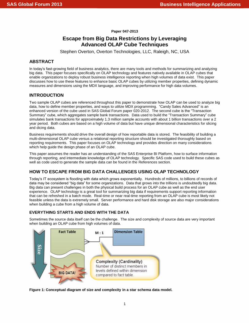
Sometimes the source data itself can be the challenge. The size and complexity of source data are very important when building an OLAP cube from high volumes of data.

Figure 1: Conceptual diagram of size and complexity in a star schema data model.

Business Intelligence ApplicationsSAS Global Forum 2013

2

As shown in Figure 1, the size of data is represented by the number of records. The complexity of data, with regards to building OLAP cubes, is determined by the relationships that exist between tables. A dimensional model naturally maintains a many-to-one relationship between fact and dimension tables. The number of distinct members that make up levels defined from dimension tables determines the complexity. As distinct member counts grow into millions, complexity increases substantially.

If possible, source data is best structured for OLAP, as well as general reporting, in a star schema model. The build process is much more efficient building an OLAP cube from a star schema because dimensions and fact tables present the data in a much more natural manner for multi-dimensional aggregation. General reporting from a dimensional model or star schema is much more efficient as well.

OLAP BUILD PROCESS CONSIDERATIONS

There are different options for building an effective OLAP cube and different considerations that must be taken into account. Working with a high volume of data forces a developer to think outside the norm to support reporting requirements but also design a cube that actually builds in time and still functions.

Overall Build Time

If the cube is completely rebuilt or incrementally updated, the availability of the OLAP cube to users for reporting is a basic requirement to consider. Larger data volumes result in larger cubes, which usually require a longer period of downtime to build as data grows.

Method of Cube Update

Completely rebuilding a cube ensures all historical data is summarized when the cube is built. A complete rebuild takes longer than an incremental update. With large data volumes it can take considerably longer. An incremental update process leaves the OLAP cube available for reporting while new data is added. Incremental updates are efficient but historical data may need to be updated or removed. Always assess the possibility of an incremental update depending on reporting requirements and the necessity to update historical data in the OLAP cube.

Frequency of Cube Updates

Going hand-in-hand with build time and method of updating, how often the cube update process occurs needs to be considered. The volatility of source data and the business necessity of having aggregate level data presented should be a major consideration.

To Build or Not to Build the NWAY

The NWAY aggregation stores all measures aggregated to the crossing of every level defined in a cube. If the cube is taking too long to build, the volume and grain of the NWAY crossing may not be feasible to build. Try disabling the

NWAY aggregation by adding the NO_NWAY option to the PROC OLAP statement. Not having the NWAY requires

additional aggregations so the cube can perform nominally. If no aggregations exist, the OLAP server will aggregate source data at run time, which can impact performance, especially when working with big data.

Divide and Conquer

Build the cube using a “divide and conquer” technique described in SAS Global Forum paper 431-2012. This process loads data into an OLAP cube in segments to avoid physical constraints and allows access while the cube is being built.

Programming Tip: During the development of an OLAP cube, limit the amount of data processed by the cube so

development cycles do not become extremely long because of high volumes of data. Use table views or subset the data into temporary tables.

BIG DATA MEANS MORE POWER!

Hardware sizing becomes a critical area when the source data volume becomes large. The two most important sizing considerations when working with big data is the volume of records to aggregate in the cube and the cardinality of the dimensions in the cube. Both have different impacts on memory and hard disk space utilization.

Memory

Higher cardinality dimensions require more memory to process and build. As the cardinality gets into millions of records, memory settings usually need tuning to manage memory more efficiently. Having more memory allocated allows the OLAP server to build dimensions more efficiently. SAS Global Forum Paper 319-2009 describes the multiple memory options that can be configured to help manage resources during the build process.


3

Hard Disk Space

As data volume grows, so does the required disk space, depending on the type of cube built. By default, OLAP defines the NWAY aggregation. This method consumes the most hard disk space, especially with big data and even more so with high cardinality dimensions. ROLAP, or relational-OLAP, requires much less disk space but impacts the end user performance because queries aggregate data on-the-fly from the source data. Aggregation tuning can help with the end user performance but also require time to build the aggregates and hard disk space to physically store the aggregate data.

IMPROVE END USER QUERY PERFORMANCE WITH AGGREGATION TUNING

The best way to improve the end user performance of an OLAP cube is to build aggregations. More aggregations result in longer build times but will improve end user performance if used properly. Here are a few keys to aggregation tuning:

Use the ARM logging feature to assess OLAP cube usage patterns from all reporting channels. Specific instructions for enabling and using the ARM logs are presented in SAS Global Forum paper 026-2012.

Working with big data naturally means longer times to aggregate data. Assess the need for certain aggregates based on usage patterns. Unnecessary aggregates can use vital hard disk space when working with big data volumes.

If source data exists in an external database such as Oracle, investigate the possibility of building external aggregation tables completely in-database. This improves the build time, especially for big data sources. Additional discussion around external aggregations is presented in SAS Global Forum paper 219-31.

Use the CONCURRENT option in the PROC OLAP statement to manage how many aggregates can be built in

parallel.

Aggregates can be defined on-the-fly without disabling access to the cube. Less complex aggregations (those with a small number of levels crossed) are built automatically from aggregations that are more complex if they exist.

ENHANCE LOGGING TO KNOW WHAT IS HAPPENING BEHIND THE SCENES

It may be necessary to learn more about what the OLAP build process is doing. To see specific memory consumption and more detailed process times, add the following code to your OLAP process.

options fullstimer;

options SASTRACE=',,,ds' sastraceloc=saslog nostsuffix;

%let syssumtrace=3;

/* Get a quick snapshot of performance related options */

proc options group=performance; run;

SAS Global Forum paper 319-2009 describes test level options which can be enabled to better understand the memory consumption of the OLAP cube build process. Additional performance options can be added to the PROC OLAP statement to manage memory consumption better and to enable very useful debugging messages. Setting

TEST_LEVEL to 26 tells the OLAP server to report details such as how much memory is consumed by each step,

specific queries used to retrieve the data, and when and how long data is being physically written inside the cube. The following code is used to produce these details for the Transaction Summary cube.

proc olap

CUBE = "/Projects/SGF2013/Cubes/Transaction Summary"

PATH = '/projects/SGF2013/cubes'

DESCRIPTION = 'Transaction Summary demo cube for SGF2013'

FACT = postgres.FACT_TRANSACTIONS

CONCURRENT = 4

ASYNCINDEXLIMIT = 2

MAXTHREADS = 2

TEST_LEVEL = 26

;

EXAMPLE OLAP CUBE BUILD PROCESS COMPARISON

For perspective, the two OLAP cubes used for demonstration purposes in this paper both aggregate over 1 billion records of sample data, but have drastically different characteristics due to different cardinalities. Both have an


4

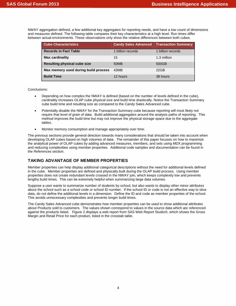
NWAY aggregation defined, a few additional key aggregates for reporting needs, and have a low count of dimensions and measures defined. The following table compares their key characteristics at a high level. Run times differ between actual environments. These observations only show the relative differences between both cubes.

Cube Characteristics Candy Sales Advanced Transaction Summary

Records in Fact Table 1 billion records 1 billion records

Max cardinality 15 1.3 million

Resulting physical cube size 50MB 500GB

Max memory used during build process 43MB 22GB

Build Time 12 hours 38 hours

Conclusions:

Depending on how complex the NWAY is defined (based on the number of levels defined in the cube), cardinality increases OLAP cube physical size and build time drastically. Notice the Transaction Summary cube build time and resulting size as compared to the Candy Sales Advanced cube.

Potentially disable the NWAY for the Transaction Summary cube because reporting will most likely not require that level of grain of data. Build additional aggregates around the analysis paths of reporting. This method improves the build time but may not improve the physical storage space due to the aggregate tables.

Monitor memory consumption and manage appropriately over time.

The previous sections provide general direction towards many considerations that should be taken into account when developing OLAP cubes based on high volumes of data. The remainder of this paper focuses on how to maximize the analytical power of OLAP cubes by adding advanced measures, members, and sets using MDX programming and reducing complexities using member properties. Additional code samples and documentation can be found in the References section.

TAKING ADVANTAGE OF MEMBER PROPERTIES

Member properties can help display additional categorical descriptions without the need for additional levels defined in the cube. Member properties are defined and physically built during the OLAP build process. Using member properties does not create redundant levels crossed in the NWAY join, which keeps complexity low and prevents lengthy build times. This can be extremely helpful when summarizing large data volumes.

Suppose a user wants to summarize number of students by school, but also wants to display other minor attributes about the school such as a school code or school ID number. If the school ID or code is not an effective way to slice data, do not define the additional levels in a dimension. Define the ID and code as member properties of the school. This avoids unnecessary complexities and prevents longer build times.

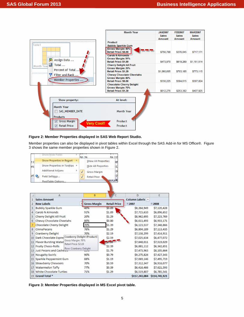
The Candy Sales Advanced cube demonstrates how member properties can be used to show additional attributes about Products sold to customers. The values shown correspond to values in the source data which are referenced against the products listed. Figure 2 displays a web report from SAS Web Report Studio®, which shows the Gross Margin and Retail Price for each product, listed in the crosstab table.


5

Figure 2: Member Properties displayed in SAS Web Report Studio.

Member properties can also be displayed in pivot tables within Excel through the SAS Add-in for MS Office®. Figure 3 shows the same member properties shown in Figure 2.

Figure 3: Member Properties displayed in MS Excel pivot table.


6

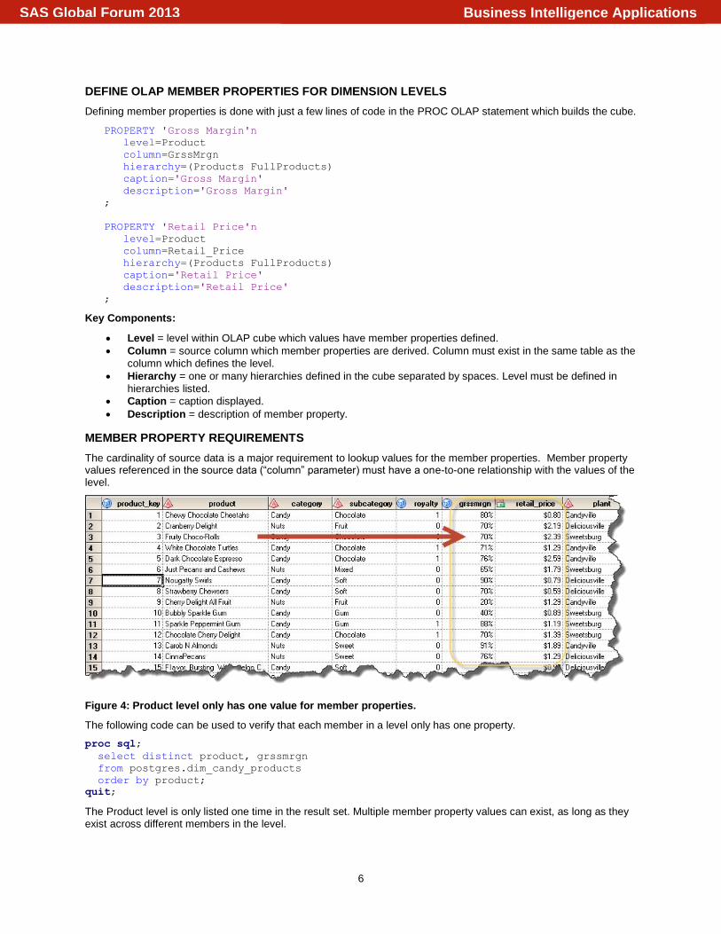
DEFINE OLAP MEMBER PROPERTIES FOR DIMENSION LEVELS

Defining member properties is done with just a few lines of code in the PROC OLAP statement which builds the cube.

PROPERTY 'Gross Margin'n

level=Product

column=GrssMrgn

hierarchy=(Products FullProducts)

caption='Gross Margin'

description='Gross Margin'

;

PROPERTY 'Retail Price'n

level=Product

column=Retail_Price

hierarchy=(Products FullProducts)

caption='Retail Price'

description='Retail Price'

;

Key Components:

Level = level within OLAP cube which values have member properties defined.

Column = source column which member properties are derived. Column must exist in the same table as the

column which defines the level.

Hierarchy = one or many hierarchies defined in the cube separated by spaces. Level must be defined in

hierarchies listed.

Caption = caption displayed.

Description = description of member property.

MEMBER PROPERTY REQUIREMENTS

The cardinality of source data is a major requirement to lookup values for the member properties. Member property values referenced in the source data (“column” parameter) must have a one-to-one relationship with the values of the level.

Figure 4: Product level only has one value for member properties.

The following code can be used to verify that each member in a level only has one property.

proc sql;

select distinct product, grssmrgn

from postgres.dim_candy_products

order by product;

quit;

The Product level is only listed one time in the result set. Multiple member property values can exist, as long as they exist across different members in the level.


7

USE MDX TO SOLVE COMPLEX BUSINESS CHALLENGES

MDX is a powerful feature of OLAP technology that brings dynamic and robust capabilities which flattened relational tables cannot produce without additional overhead or infrastructure changes. MDX statements can define custom groups of dimension values in members and sets. MDX also brings many useful functions to define custom measures, measures which reference different aggregate levels within the cube, and even measures which reference other measures.

Did You Know? MDX stands for Multi-Dimensional eXpression

MDX BASICS

The key to writing MDX statements is to understand how members and values are referenced syntactically and how to relate different levels of an OLAP cube. There are multiple ways to reference data within a cube. This paper will use a few basic MDX functions and techniques to provide high-level guidance. Check the References section for other functions and techniques and more information on MDX data types.

Here are some useful tips when working with MDX coding:

Defining additional metrics in an OLAP cube using MDX is very effective when working with big data because it adds no additional size to the physical data or cube. MDX measures process aggregate data in the cube at run time. If an OLAP cube is utilized to summarize and report big data, try defining base level measures in the source data and perform as many calculations as possible using MDX in the cube.

MDX code can be submitted and defined at any point and not affect end users because the OLAP cube does not have to be physically rebuilt or disabled. MDX measures, members, and sets are simply definitions of how to slice data in the OLAP cube.

Always try to define a TIME dimension in the OLAP cube. Many useful MDX functions require a dimension with a type equal to TIME in order to perform the query. Logically it makes sense in most cases to know when a particular measure occurred.

To learn MDX syntax on your own, use SAS Enterprise Guide® to manipulate an OLAP cube, then right-click to view the result set with the MDX editor. Try creating your own measures, members, and sets within Enterprise Guide to easily test your knowledge and gain experience.

When faced with challenging measures, take baby steps and try to build MDX in small pieces first. Then put the pieces together to build a final measure or series of measures. For example, build the numerator and the denominator as separate measures. Then define another custom measure to perform the division.

MDX measures are commonly based on OLAP aggregations of basic numeric measures defined in the cube. When referring to a “member” or “set”, another way to think of the result is what measure is at that crossing or aggregation level.

For security purposes, it is possible to hide certain measures, members, or even slices of data within an OLAP cube. This is managed in SAS metadata and can be performed using SAS OLAP Cube Studio in SAS 9.2® or later.

Since OLAP is aggregate level, calculations must occur based on the aggregate view of a measure. In other

words, calculations which must be done before the SUM or COUNT of a measure must be done to the source

data directly before the cube is built. A good example is a weighted average. The weighted numerator must be multiplied before data enters the OLAP cube, then division can occur as an MDX measure based on the two aggregations of the weighted numerator and denominator.

Navigation functions are used to reference different members at different levels dynamically. Common functions are:

o .CurrentMember – Returns the current member aggregate in of a slice of data which can be used

to define measures based on the relative position in a hierarchy.

o .PrevMember – Returns the previous member aggregate in a hierarchy. Can be used in

conjunction with .CurrentMember to compare measures between members.

o .Parent – Returns the parent level aggregate in a hierarchy.

MDX SOLUTIONS TO COMMON CHALLENGES

The following subsections describe how to take advantage of MDX by demonstrating key functions and techniques to tackle specific business challenges. Each subsection will describe the challenge and breakdown the MDX used to demonstrate the results.

Rolling Time Set

OLAP cubes are unique because they can have a single data item which changes dynamically over time as data is added to the cube. This gives report builders the ability to present dynamic data in reports without the need to


8

change filters. A rolling time set is a dynamic set of dimension members which are queried at run time using the

TAIL or HEAD function.

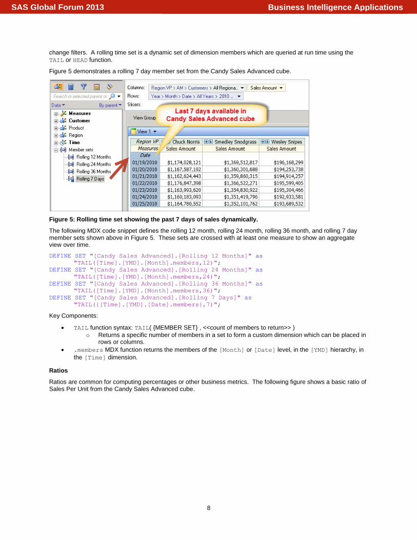
Figure 5 demonstrates a rolling 7 day member set from the Candy Sales Advanced cube.

Figure 5: Rolling time set showing the past 7 days of sales dynamically.

The following MDX code snippet defines the rolling 12 month, rolling 24 month, rolling 36 month, and rolling 7 day member sets shown above in Figure 5. These sets are crossed with at least one measure to show an aggregate view over time.

DEFINE SET "[Candy Sales Advanced].[Rolling 12 Months]" as

"TAIL([Time].[YMD].[Month].members,12)";





DEFINE SET "[Candy Sales Advanced].[Rolling 7 Days]" as

"TAIL({[Time].[YMD].[Date].members},7)";

Key Components:

TAIL function syntax: TAIL( {MEMBER SET} , <<count of members to return>> )

o Returns a specific number of members in a set to form a custom dimension which can be placed in rows or columns.

.members MDX function returns the members of the [Month] or [Date] level, in the [YMD] hierarchy, in

the [Time] dimension.

Ratios

Ratios are common for computing percentages or other business metrics. The following figure shows a basic ratio of Sales Per Unit from the Candy Sales Advanced cube.


9

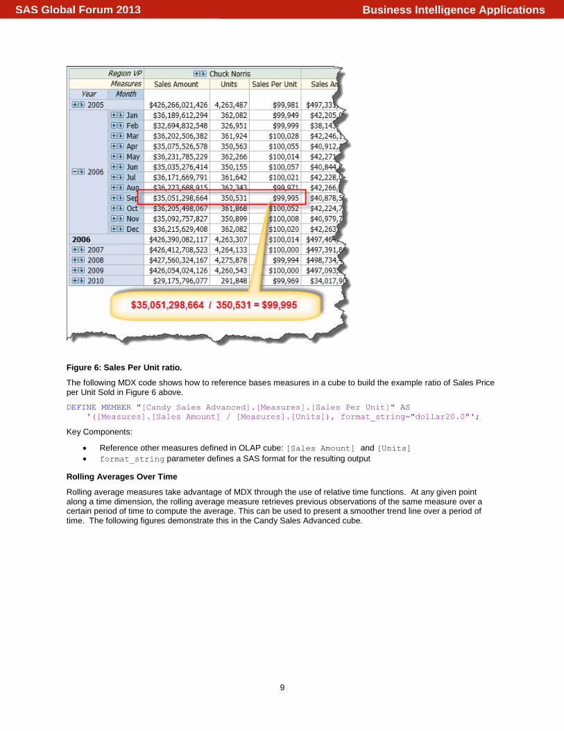
Figure 6: Sales Per Unit ratio.

The following MDX code shows how to reference bases measures in a cube to build the example ratio of Sales Price per Unit Sold in Figure 6 above.

DEFINE MEMBER "[Candy Sales Advanced].[Measures].[Sales Per Unit]" AS

'([Measures].[Sales Amount] / [Measures].[Units]), format_string="dollar20.0"';

Key Components:

Reference other measures defined in OLAP cube: [Sales Amount] and [Units]

format_string parameter defines a SAS format for the resulting output

Rolling Averages Over Time

Rolling average measures take advantage of MDX through the use of relative time functions. At any given point along a time dimension, the rolling average measure retrieves previous observations of the same measure over a certain period of time to compute the average. This can be used to present a smoother trend line over a period of time. The following figures demonstrate this in the Candy Sales Advanced cube.


10

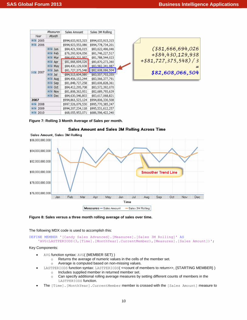
Figure 7: Rolling 3 Month Average of Sales per month.

Figure 8: Sales versus a three month rolling average of sales over time.

The following MDX code is used to accomplish this:

DEFINE MEMBER '[Candy Sales Advanced].[Measures].[Sales 3M Rolling]' AS

'AVG(LASTPERIODS(3,[Time].[MonthYear].CurrentMember),[Measures].[Sales Amount])';

Key Components:

AVG function syntax: AVG( {MEMBER SET} )

o Returns the average of numeric values in the cells of the member set. o Average is computed based on non-missing values.

LASTPERIODS function syntax: LASTPERIODS( <<count of members to return>>, {STARTING MEMBER} )

o Includes supplied member in returned member set. o Can specify additional rolling average measures by setting different counts of members in the

LASTPERIODS function.

The [Time].[MonthYear].CurrentMember member is crossed with the [Sales Amount] measure to


11

aggregate values in the MDX statement. These two MDX data references are crossed by separating with a comma in an expression. A good practice is to enclose these crossings in parenthesis to organize code.

.CurrentMember function dynamically returns the current member along the supplied hierarchy, which is

the [Time].[MonthYear] hierarchy in this example. In other words, for each month in Figure 6 and Figure

7, average the total sales for the given month with the previous 2 months.

Percent Change Over Time

Analyzing the growth of a measure by percentage provides a relative way to compare metrics over time. It is also

another great example of the relative dynamic power of MDX measures. Using the same .CurrentMember logic

from the previous example, this example will extend further and use the .PrevMember function.

The following screenshot in Figure 9 shows percent growth of sales month over month in the Candy Sales Advanced cube using MDX measures.

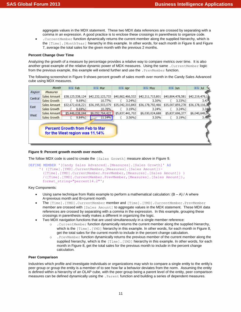
Figure 9: Percent growth month over month.

The follow MDX code is used to create the [Sales Growth] measure above in Figure 9.

DEFINE MEMBER '[Candy Sales Advanced].[Measures].[Sales Growth]' AS

'( ([Time].[YMD].CurrentMember,[Measures].[Sales Amount])-

([Time].[YMD].CurrentMember.PrevMember,[Measures].[Sales Amount]) )

/([Time].[YMD].CurrentMember.PrevMember,[Measures].[Sales Amount]),

format_string="percent14.2"';

Key Components:

Using same technique from Ratio example to perform a mathematical calculation: (B – A) / A where A=previous month and B=current month.

The [Time].[YMD].CurrentMember member and [Time].[YMD].CurrentMember.PrevMember

member are crossed with [Sales Amount] to aggregate values in the MDX statement. These MDX data

references are crossed by separating with a comma in the expression. In this example, grouping these crossings in parenthesis really makes a different in organizing the logic.

Two MDX navigation functions that are used simultaneously in a single member reference:

o .CurrentMember function dynamically returns the current member along the supplied hierarchy,

which is the [Time].[YMD] hierarchy in this example. In other words, for each month in Figure 8,

get the total sales for the current month to include in the percent change calculation.

o .PrevMember function dynamically returns the previous member of the current member along the

supplied hierarchy, which is the [Time].[YMD] hierarchy in this example. In other words, for each

month in Figure 8, get the total sales for the previous month to include in the percent change calculation.

Peer Comparison

Industries which profile and investigate individuals or organizations may wish to compare a single entity to the entity’s peer group or group the entity is a member of to see how far a behavior deviates from the norm. Assuming the entity is defined within a hierarchy of an OLAP cube, with the peer group being a parent level of the entity, peer comparison

measures can be defined dynamically using the .Parent function and building a series of dependent measures.


12

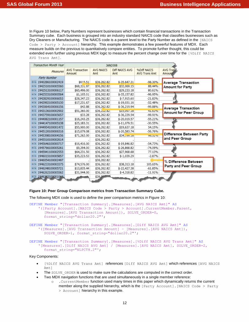
In Figure 10 below, Party Numbers represent businesses which contain financial transactions in the Transaction Summary cube. Each business is grouped into an industry standard NAICS code that classifies businesses such as

Dry Cleaners or Manufacturing. The NAICS code is a parent level to the Party Number as defined in the [NAICS

Code > Party > Account] hierarchy. This example demonstrates a few powerful features of MDX. Each

measure builds on the previous to quantitatively compare entities. To promote further thought, this could be

extended even further using previous MDX logic to measure the percent change over time for the [%Diff NAICS

AVG Trans Amt].

Figure 10: Peer Group Comparison metrics from Transaction Summary Cube.

The following MDX code is used to define the peer comparison metrics in Figure 10:

DEFINE Member "[Transaction Summary].[Measures].[AVG NAICS Amt]" AS

'([Party Account].[NAICS Code > Party > Account].CurrentMember.Parent,

[Measures].[AVG Transaction Amount]), SOLVE_ORDER=0,

format_string="dollar20.2"';

DEFINE Member "[Transaction Summary].[Measures].[Diff NAICS AVG Amt]" AS

'([Measures].[AVG Transaction Amount] - [Measures].[AVG NAICS Amt]),

SOLVE_ORDER=1, format_string="dollar20.2"';

DEFINE Member "[Transaction Summary].[Measures].[%Diff NAICS AVG Trans Amt]" AS

'[Measures].[Diff NAICS AVG Amt] / [Measures].[AVG NAICS Amt], SOLVE_ORDER=2,

format_string="NLPCT8.2"';

Key Components:

[%Diff NAICS AVG Trans Amt] references [Diff NAICS AVG Amt] which references [AVG NAICS Amt]

The SOLVE_ORDER is used to make sure the calculations are computed in the correct order.

Two MDX navigation functions that are used simultaneously in a single member reference:

o .CurrentMember function used many times in this paper which dynamically returns the current

member along the supplied hierarchy, which is the [Party Account].[NAICS Code > Party

> Account] hierarchy in this example.


13

o .Parent function dynamically returns the parent level member to aggregate along the supplied

hierarchy, which is the [Party Account].[NAICS Code > Party > Account] hierarchy in

this example. In other words, for each party, aggregate the level above the party, which is the

group of parties, which in this example is the [NAICS Code].

Additional discussion on custom MDX measures, members, and sets can be found in the SAS Global Forum paper 433-2011 listed the references section of this paper. Additional reading for MDX navigation functions can also be found in the references section below.

CONCLUSION

OLAP can be a very daunting technology at first. The goal of this paper is to make it seem less daunting and empower SAS programmers with the knowledge and advanced skills to tackle complex business challenges in today’s world. One of the biggest advantages of OLAP is the ability to present aggregate data extremely fast and have the ability to tune performance over time. Another major advantage of OLAP is the underlying MDX programming language to query cubes dynamically and define unique measures, members, and sets. As data becomes “big data”, OLAP can be an effective way to summarize and analyze business metrics. With the techniques and guidelines described in this paper, it is possible to escape from big data challenges and deliver powerful analysis tools to make better decisions based on quantitative results.

REFERENCES

SAS code which builds sample data and demonstrates the OLAP and MDX techniques described in this paper are available at http://www.stephenoverton.net/SASCode/SGF2013/.

Miles, Brian and Zenick, Ben. March 2006. Paper 219-31. “Beyond the Basics: Advanced OLAP Techniques.”

SUGI 31. San Francisco, CA. Available at: http://www2.sas.com/proceedings/sugi31/219-31.pdf.

Simmons, Mary and Wilkie, Michelle. March 2009. Paper 219-2009. “Best Practice: Optimizing the cube build

process in SAS® 9.2.” SAS Global Forum 2009. Washington, DC. Available at

http://support.sas.com/resources/papers/proceedings09/319-2009.pdf.

Overton, Stephen and Stines, Bryan. April 2011. Paper 433-2011. “Measures, Members, and Sets, Oh My!

Advanced OLAP Techniques.” SAS Global Forum 2011. Las Vegas, NV. Available at


Overton, Stephen. April 2012. Paper 020-2012. “Lost in Wonderland? Methodology for a Guided Drill-Through

Analysis Out of the Rabbit Hole.” SAS Global Forum 2012. Orlando, FL. Available at


Overton, Stephen. April 2012. Paper 431-2012. “10,000 Leagues of Data... Divide and Conquer OLAP Cubes:

Best Practices for High Volumes of Data.” SAS Global Forum 2012. Orlando, FL. Available at


Petrova, Tatyana. April 2012. Paper 026-2012. “SAS OLAP Cube Tuning and Query Performance

Optimization.” SAS Global Forum 2012. Orlando, FL. Available at


SAS Support. “Coalescing Cube Aggregations.” March 7, 2013. Available at http://support.sas.com/documentation/cdl/en/olapug/59574/HTML/default/viewer.htm#a003241634.htm.

SAS Support. “Updating a Cube In-Place.” March 7, 2013. Available at http://support.sas.com/documentation/cdl/en/olapug/59574/HTML/default/viewer.htm#a003241629.htm.

Wikipedia. “MultiDimensional eXpressions.” March 7, 2013. Available at: http://en.wikipedia.org/wiki/MultiDimensional_eXpressions.

MDXpert.com. “MDXpert.com.” March 7, 2013. Available at: http://mdxpert.com/.

Wikipedia. “Star Schema.” March 7, 2013. Available at http://en.wikipedia.org/wiki/Star_schema.


http://www.stephenoverton.net/SASCode/SGF2013/

http://www2.sas.com/proceedings/sugi31/219-31.pdf

http://support.sas.com/resources/papers/proceedings09/319-2009.pdf





http://support.sas.com/documentation/cdl/en/olapug/59574/HTML/default/viewer.htm#a003241634.htm

http://support.sas.com/documentation/cdl/en/olapug/59574/HTML/default/viewer.htm#a003241629.htm

http://en.wikipedia.org/wiki/MultiDimensional_eXpressions

http://mdxpert.com/

http://en.wikipedia.org/wiki/Star_schema

14

CONTACT INFORMATION

Your comments and questions are valued and encouraged. Contact the author at:

Stephen Overton

Overton Technologies, LLC (http://www.overtontechnologies.com) Email: [email protected] Website: http://www.stephenoverton.net LinkedIn: http://www.linkedin.com/in/overton

SAS and all other SAS Institute Inc. product or service names are registered trademarks or trademarks of SAS Institute Inc. in the USA and other countries. ® indicates USA registration.

Other brand and product names are trademarks of their respective companies.


http://www.overtontechnologies.com/

mailto:[email protected]

http://www.stephenoverton.net/

http://www.linkedin.com/in/overton

Paper 047-2013: Escape from Big Data Restrictions by Leveraging ...

Documents

Transcript of Paper 047-2013: Escape from Big Data Restrictions by Leveraging ...