Full Terms & Conditions of access and use can be found athttp://www.tandfonline.com/action/journalInformation?journalCode=ujrs20

Download by: [Oregon State University] Date: 07 June 2016, At: 10:26

Canadian Journal of Remote SensingJournal canadien de télédétection

ISSN: 0703-8992 (Print) 1712-7971 (Online) Journal homepage: http://www.tandfonline.com/loi/ujrs20

Imputation of Individual Longleaf Pine (Pinuspalustris Mill.) Tree Attributes from Field andLiDAR Data

Carlos A. Silva, Andrew T. Hudak, Lee A. Vierling, E. Louise Loudermilk,Joseph J. O'Brien, J. Kevin Hiers, Steve B. Jack, Carlos Gonzalez-Benecke,Heezin Lee, Michael J. Falkowski & Anahita Khosravipour

To cite this article: Carlos A. Silva, Andrew T. Hudak, Lee A. Vierling, E. Louise Loudermilk,Joseph J. O'Brien, J. Kevin Hiers, Steve B. Jack, Carlos Gonzalez-Benecke, Heezin Lee, MichaelJ. Falkowski & Anahita Khosravipour (2016): Imputation of Individual Longleaf Pine (Pinuspalustris Mill.) Tree Attributes from Field and LiDAR Data, Canadian Journal of Remote Sensing,DOI: 10.1080/07038992.2016.1196582

To link to this article: http://dx.doi.org/10.1080/07038992.2016.1196582

Accepted author version posted online: 03Jun 2016.Published online: 03 Jun 2016.

Submit your article to this journal

Article views: 11

View related articles

View Crossmark data

ACCEPTED MANUSCRIPT

ACCEPTED MANUSCRIPT 1

Imputation of Individual Longleaf Pine (Pinus palustris Mill.) Tree Attributes from Field

and LiDAR Data

Carlos A. Silva1,*

, Andrew T. Hudak2, Lee A. Vierling

1, E. Louise Loudermilk

3, Joseph J.

O’Brien3, J. Kevin Hiers

4, Steve B. Jack

5, Carlos Gonzalez-Benecke

6, Heezin Lee

7, Michael J.

Falkowski8, and Anahita Khosravipour

9

1 Department of Forest, Rangeland, and Fire Sciences, College of Natural Resources, University

of Idaho, Moscow, ID 83843, USA

2 USDA Forest Service, Rocky Mountain Research Station, Moscow, ID 83843, USA

3 USDA Forest Service, Southern Research Station, Athens, GA 30602, USA

4 Office of Environmental Stewardship, University of the South, Sewanee, TN 37383, USA

5 Joseph W. Jones Ecological Research Center, 3988 Jones Center Drive, Newton, GA 39870-

8522, USA

6 Department of Forest Engineering, Resources and Management, Oregon State University,

Corvallis, OR, 97331, USA

7 Department of Earth and Planetary Science, University of California, Berkeley, CA, 94720,

USA

8 Department of Ecosystem Science and Sustainability, Colorado State University, Fort Collins,

CO 80523, USA

9 Department of Natural Resources, University of Twente, 7500 AE, Enschede, The Netherlands

Received 16 October 2015. Accepted 13 March 2016.

*Corresponding author e-mail: csilva@uidaho.edu

Dow

nloa

ded

by [

Ore

gon

Stat

e U

nive

rsity

] at

10:

26 0

7 Ju

ne 2

016

ACCEPTED MANUSCRIPT

ACCEPTED MANUSCRIPT 2

Abstract

Light Detection and Ranging (LiDAR) has demonstrated potential for forest inventory at

the individual tree-level. The aim in this study was to predict individual tree height (Ht; m), basal

area (BA; m2) and stem volume (V; m

3) attributes using Random Forest k- nearest neighbor (RF

k-NN) imputation and individual tree-level based metrics extracted from a LiDAR-derived

canopy height model (CHM) in a longleaf pine (Pinus palustris Mill.) forest in southwestern

Georgia, USA. We developed a new framework for modeling tree-level forest attributes that was

comprised of three steps: (1) individual tree detection, crown delineation and tree-level based

metrics computation from LiDAR-derived CHM; (2) automatic matching of LiDAR-derived

trees and field-based trees for a regression modeling step using a novel algorithm; and (3) RF k-

NN imputation modeling for estimating tree-level Ht, BA, and V, and subsequent summarization

of these metrics at the plot- and stand-levels. RMSDs for tree-level Ht, BA and V were 2.96%,

58.62% and 8.19%, respectively. Although BA estimation accuracy was poor because of the

longleaf pine growth habit, individual tree locations, Ht, and V were estimated with high

accuracy, especially in low canopy cover conditions. Future efforts based on the findings could

help to improve the estimation accuracy of individual tree-level attributes like BA.

Résumé

Le lidar a démontré son potentiel pour l'inventaire forestier à l’échelle de l’arbre. Le but

de cette étude était de prédire la hauteur individuelle des arbres (Ht; m), la surface terrière (BA;

m2) et le volume des tiges (V; m

3) en utilisant une imputation basée sur la méthode des forêts

aléatoires et des k plus proches voisins (RF k-NN; Random Forest k-nearest neighbor) et de

mesures à l’échelle de l’arbre extraites à partir d'un modèle de la hauteur de la canopée (MHC)

Dow

nloa

ded

by [

Ore

gon

Stat

e U

nive

rsity

] at

10:

26 0

7 Ju

ne 2

016

ACCEPTED MANUSCRIPT

ACCEPTED MANUSCRIPT 3

dérivés du lidar dans une forêt de pins des marais (Pinus palustris Mill.) dans le sud-ouest de la

Géorgie, aux États-Unis. Nous avons développé un nouveau cadre pour la modélisation des

attributs forestiers à l’échelle de l'arbre composé de trois étapes : 1. la détection des arbres

individuels, la délimitation des couronnes et le calcul de paramètres à l’échelle de l'arbre à partir

de modèles MHC obtenus à partir du lidar; 2. la mise en correspondance automatique entre les

arbres obtenus à partir du lidar et les arbres observés sur le terrain pour une étape de

modélisation de régression en utilisant un nouvel algorithme; et 3. l'imputation par modélisation

en utilisant RF k-NN pour estimer la Ht, la BA et le V à l’échelle de l'arbre et la synthèse

ultérieure de ces mesures à l’échelle de la parcelle et du peuplement. Les REQM pour la Ht, la

BA et le V à l’échelle de l'arbre étaient de 2,96 %, 58,62 % et 8,19 %, respectivement. Bien que

la précision de l'estimation de la BA fût faible en raison du port et du mode de croissance des

pins des marais, l’emplacement des arbres individuels, la Ht et le V ont été estimés avec une

grande précision, en particulier dans des conditions de faible couverture de la canopée. Les

efforts futurs basés sur ces résultats pourraient aider à améliorer la précision de l'estimation des

attributs à l’échelle de l’arbre comme la BA.

Dow

nloa

ded

by [

Ore

gon

Stat

e U

nive

rsity

] at

10:

26 0

7 Ju

ne 2

016

ACCEPTED MANUSCRIPT

ACCEPTED MANUSCRIPT 4

Introduction

Longleaf pine (Pinus palustris Mill.) was once one of the most ecologically important

tree species in the Southern United States (Oswalt et al., 2012). Historically, longleaf pine forests

spanned an estimated area of 92 million acres (Frost 2006) and were among the most extensive

ecosystems in North America (Landers et al. 1995). Today, only four percent of these longleaf

pine forests remain (Franklin 2008).

Fire is one of the dominant forces that shapes the longleaf pine landscape (Dobbs 2011).

Longleaf pine is dependent on fire for successful regeneration and for suppressing hardwood

growth (Loudermilk et al., 2011). However, due to fire suppression, much of the remaining

longleaf pine forest is in poor or degraded condition. As a result, there has been tremendous

interest in longleaf pine conservation, management and restoration (Brockway, 2005).

Successful management of these forests can have sustainable results, as longleaf pines

can produce quality wood products when grown in a variety of densities (Franklin 2008).

Accurate measures of forest attributes like tree density (tree/ha), and attributes such as height

(Ht), basal area (BA), and stem volume (V) that are used at the tree-, plot- and stand-levels, are

essential to management and conservation practices in longleaf pine forests. The most accurate

method of estimating these attributes is to physically sample them in the field. However,

individual tree field measurements over large areas are limited by budgets and time, making

them impractical.

Airborne Light Detection and Ranging (LiDAR) systems have become the dominant

remote sensing technique for plot- and stand-level forest inventory, mainly due to the fact that

Dow

nloa

ded

by [

Ore

gon

Stat

e U

nive

rsity

] at

10:

26 0

7 Ju

ne 2

016

ACCEPTED MANUSCRIPT

ACCEPTED MANUSCRIPT 5

this technology can quickly provide highly accurate and spatially detailed information about

forest attributes across entire forested landscapes (Silva et al. 2014). Increased interest, dataset

availability, and technological improvements have greatly expanded the use of LiDAR

technologies in forestry over the past decade (Saremi et al. 2014, Hudak et al. 2014, Hansen et al.

2015).

The use of airborne LiDAR to retrieve forest attributes at the tree-level is promising,

however not as widely studied as plot- or stand-level approaches. In a tree-level based modeling

approach, individual tree attributes are usually predicted through three steps: (1) individual tree

detection and metrics extraction, (2) LiDAR- and field-based tree matching and (3) modeling and

prediction. The accurate prediction of tree-level attributes is highly dependent on the methods

used to detect and extract individual tree metrics and forest structure as well (Kankare et al.

2015).

A LiDAR-derived Canopy Height Model (CHM) can be used for detecting individual

trees, delineating tree crowns, and subsequently estimating biophysical attributes such as

biomass and stem volume (Popescu et al. 2003, Popescu, 2007, Falkowski et al. 2008, 2009,

Vauhkonen et al. 2012, Hu et al. 2014, Duncanson et al. 2014, 2015, Kankare et al. 2015). There

are a variety of approaches used to detect and delineate individual trees from LiDAR-derived

CHMs. These include identifying local maxima (Popescu et al. 2003, Weinacker et al. 2004,

Falkowski et al. 2008, 2009) for tree detection, as well as region-growing (Hyyppä et al. 2001,

Solberg et al. 2006, Pang et al. 2008), valley-following (Leckie et al. 2003) and watershed (Chen

et al. 2006, Jing et al. 2012) for delineation.

Dow

nloa

ded

by [

Ore

gon

Stat

e U

nive

rsity

] at

10:

26 0

7 Ju

ne 2

016

ACCEPTED MANUSCRIPT

ACCEPTED MANUSCRIPT 6

In addition to the individual tree detection method and forest structure, the accurate

prediction of forest attributes at the tree level is also highly dependent on the modeling technique

applied (Vauhkonen et al. 2010). Examples of the existing methods for modeling forest attributes

at the tree-level from LiDAR data are both parametric (Chen et al., 2007) and non-parametric

(Breidenbach et al. 2010, Vauhkonen et al. 2010, Vauhkonen et al. 2012). Saarinen et al. (2014),

Vastaranta et al. (2014) and Kankare et al. (2015) have been recently tested k-nearest neighbor

(k-NN) imputation for forest inventory modeling at the tree-level. In most cases however, k-NN

imputation, as a nonparametric method, has commonly been used to predict forest inventory

attributes at the plot- or stand-levels (Falkowski et al., 2010, Hudak et al., 2014, Racine et al.,

2014). For example, Hudak et al. (2008) evaluated nine k-NN imputation methods and LiDAR

data for imputing plot-level BA and tree density (TD) of 11 conifer species occurring in mixed-

conifer forests of north-central Idaho, USA. Racine et al. (2014) used LiDAR data and k-NN

imputation to estimate plot age across a managed boreal forest in Quebec, Canada, while Fekety

et al. (2015) used repeated field and LiDAR survey data to assess the feasibility of predicting

forest inventory attributes across space and time in a conifer forest in Northern Idaho, USA.

The aforementioned studies integrated LiDAR and field data in an area based k-NN

imputation to predict forest attributes at the plot- or stand-levels. However, accurate

characterization of the forest at the individual tree-level not only enhances conventional and

LiDAR area-based forest inventory, but also extends its applications in disciplines where greater

detail is valued, such as ecology, wildlife habitat or biodiversity applications (Goetz et al., 2007,

Hinsley et al., 2002, Vierling et al., 2008).

Dow

nloa

ded

by [

Ore

gon

Stat

e U

nive

rsity

] at

10:

26 0

7 Ju

ne 2

016

ACCEPTED MANUSCRIPT

ACCEPTED MANUSCRIPT 7

Given that only a fraction of the historic longleaf pine forest ecosystem range remains

today, accurate characterization and spatial distribution of individual trees are critical for

sustainable forest management and for ecological and environmental protection in longleaf pine

forests. Our goal in this study was to predict individual tree-level attributes using k-NN

imputation and individual tree LiDAR-based metrics in a longleaf pine forest in southwestern

Georgia, USA. Our first aim therefore was to evaluate the ability of LiDAR to accurately detect

individual trees and determine treetop height (HMAX, m) and crown area (CA, m2) that are

subsequently used for predicting tree attributes. Our second aim was to predict individual tree Ht

(m), BA (m2) and V (m

3) attributes from HMAX and CA metrics using k-NN imputation, and

evaluate its accuracy and precision. This investigation is based on the hypothesis that LiDAR

technology and k-NN imputation modeling approach can feasibly provide precise and accurate

estimates of these tree attributes in the open canopy structure that is typical of healthy longleaf

pine forests.

Material and methods

Study area

The study area for this project is located at Ichauway, an 11,700 ha reserve of the Joseph

W. Jones Ecological Research Center in southwestern Georgia, USA (Figure 1). The area is

characterized by a humid subtropical climate (Christensen 1981) with a mean annual

precipitation of 131 cm fairly evenly spread throughout the year. Mean daily temperatures range

from 21◦C to 34◦C in the summer and 5◦C to 17◦C in the winter (Loudermilk et al., 2011).

Elevation ranges from 6.23 to 33.66 m, and the soils are characterized as paleudults, kandiudults

and hapludults with some localized quartzipsamments (Kirkman et al. 2004). The Ichauway

Dow

nloa

ded

by [

Ore

gon

Stat

e U

nive

rsity

] at

10:

26 0

7 Ju

ne 2

016

ACCEPTED MANUSCRIPT

ACCEPTED MANUSCRIPT 8

reserve has an extensive tract of second-growth longleaf pine managed with low-intensity,

dormant-season prescribed fires at a frequency of about 1–3 years since 1945 (Loudermilk et al.,

2011).

In this study, vegetation structure is characterized by an open canopy longleaf pine forest

(Figure 1. A, B) and a wiregrass-dominated ground cover maintained under a high frequency fire

regime (Figure 1. C). Maintaining a high frequency fire regime through repeated application of

prescribed fire is a top management goal at Ichauway, with occasional individual tree selection

harvesting for management and research purposes in the natural, second-growth longleaf forests

(Palik et al. 2003).

Field Data Collection

The field measurements were carried out from March to July 2009. A total of 15

rectangular plots (about 4 ha each) were established in three stands: CNT, NE, and NW (Figure 1

D). All plots were geo-referenced with a geodetic GPS with differential correction capability

(Trimble Nomad) with an external Hemisphere Crescent A100 antenna, and had a horizontal

accuracy of < 0.6 m with differential GPS (DGPS) and < 2.5 m without DGPS in open canopy,

and 1-2 m accuracy with DGPS under forest canopy. All trees were measured for DBH using

calipers (two perpendicular measurements at right angles, averaged) or a steel diameter tape, and

for Ht using a LaserTech Impulse 200. We also geo-located (UTM E, N) them using the GPS

mentioned above, and from these measures a field stem-map was created. In a few instances

DGPS was not able to resolve locations of multiple small trees in areas with high stocking, and

tree locations were recorded by establishing a known DGPS point and then measuring the

distance (3-5 cm accuracy) and azimuth (± 0.3 degree accuracy) to those trees with the Impulse

Dow

nloa

ded

by [

Ore

gon

Stat

e U

nive

rsity

] at

10:

26 0

7 Ju

ne 2

016

ACCEPTED MANUSCRIPT

ACCEPTED MANUSCRIPT 9

200 and MapStar Compass module, respectively. The mean longleaf pine tree Ht and DBH

measured in our study area was 22.95 (±4.88) m and 32.87 (±13.30) cm, respectively, and the

number of trees per hectare (N/ha) was approximately 147 (±29) trees. A statistical summary of

the tree density, Ht and DBH field measurements are presented in Error! Reference source not

found..

The outside-bark V was obtained via a longleaf pine allometric equation according to

Gonzalez-Benecke et al. (2014) (equation 1). The equation has a coefficient of determination

(R2) of 0.78 and absolute and relative RMSE of 0.17 m

3 and 38.21%, respectively.

ln(V) = -9.944543 + 3.123691 * ln(Ht) (1)

In addition to V, tree-level BA was also computed. Statistical summaries of the reference

BA and V calculations are presented in Table 2.

LiDAR Data and Pre-processing

LiDAR data were acquired using an Optech GEMINI Airborne Laser Terrain Mapper

(ALTM) mounted in a twin-engine Cessna Skymaster (Tail Number N337P). The survey was

carried out on March 5, 2008. LiDAR flight parameters are presented in Error! Reference

source not found..

LiDAR pre-processing was performed using US Forest Service FUSION/LDV 3.42 software

(McGaughey 2015) and LAStools (Isenburg 2015). The workflow is graphically shown in Figure

2A. First, in FUSION/LDV, the quality of the LiDAR data set was visually evaluated, and a

simple report using Catalog tool was generated. A filtering algorithm based on Kraus and Pfeifer

(1998) was applied to differentiate between ground and non-ground returns. DTMs were

generated using the classified ground points with a spatial resolution of 1.0 m using the

Dow

nloa

ded

by [

Ore

gon

Stat

e U

nive

rsity

] at

10:

26 0

7 Ju

ne 2

016

ACCEPTED MANUSCRIPT

ACCEPTED MANUSCRIPT 10

GridSurfaceCreate function. The CanopyModel tool was then used to interpolate vegetation

points and to generate DSMs with a spatial resolution of 0.5 m. Afterwards, the ClipData tool

was applied with the height and dtm switches to normalize heights and to assure that the z

coordinate for each point corresponded to the height above ground and not the orthometric

elevation of the single point. The PolyClipData tool was then used to make a subset of the

LiDAR points within each of the 15 in situ-measured test plots. The CloudMetrics tool with a

height and cover thresholds of 1.37 m (Nilsson, 1996) were used to compute the canopy cover

(COV, %), within sample plots. COV was calculated as the number of LiDAR first returns above

1.37 m, divided by the total number of first returns. Such LiDAR-derived CHM often contain

height irregularities within individual tree crowns--so-called data pits--which reduce accuracy in

tree detection and subsequent extraction of biophysical parameters (Gaveau and Hill, 2003,

Shamsoddini et al. 2013). Therefore, the pit-free algorithm, developed by Khosravipour et al.

(2014) was used to generate a pit-free CHM at 0.5 m spatial resolution though a workflow

implemented in LAStools (Isenburg 2015).

Individual tree detection and HMAX extraction

Individual tree detection was performed in R (R Development Core Team 2015) using

the FindTreesCHM function from the rLiDAR package (Silva et al. 2015). The FindTreesCHM

function uses a local maximum algorithm to search for treetops in the CHM trough a moving

window with a fixed treetop window size (TWS) (Wulder, et al. 2000). To achieve optimal tree

detection we tested three TWS (3x3, 5x5, and 7x7) first on an unsmoothed CHM, and then on a

CHM smoothed by a mean smooth filter with fixed smoothing window size (SWS) of 3x3 and

Dow

nloa

ded

by [

Ore

gon

Stat

e U

nive

rsity

] at

10:

26 0

7 Ju

ne 2

016

ACCEPTED MANUSCRIPT

ACCEPTED MANUSCRIPT 11

5x5. Even when the smoothed CHM option was used to find trees, the treetop heights (HMAX)

were extracted from the unsmoothed CHM.

A total of 15 test subplots (30x30 m) were randomly situated within each of the 15 plots

(1 subplot per plot), and the number of trees detected (NTD) per subplot from LiDAR were

manually compared with field-based data and evaluated in terms of true positive (TP, correct

detection), false negative (FN, omission error) and false positive (FP, commission error). The

accuracy of the detection was further evaluated for recall (r), precision (p) and F-score (F)

according to Li et al. (2012), using the following equations (Goutte and Gaussier, 2005,

Sokolova et al., 2006):

(2)

(3)

(4)

Note that recall is inversely related to omission error and represents the tree detected rate.

Precision is inversely related to commission error and describes the rate of correct detections. F-

score is used to represent the harmonic mean of recall and precision, which takes both

commission and omission errors into consideration. Hence, a higher F-score indicates that both

commission and omission errors are lower (Li et al. 2012). Recall, precision and F-score ranges

from 0 to 1, and the F-score will become higher with higher p and r values.

Dow

nloa

ded

by [

Ore

gon

Stat

e U

nive

rsity

] at

10:

26 0

7 Ju

ne 2

016

ACCEPTED MANUSCRIPT

ACCEPTED MANUSCRIPT 12

Individual tree crown delineation and crown area computation

Tree crown delineation was also performed in R using the ForestCAS function from the

rLiDAR package (Silva et al. 2015). Inputs to this process were the smoothed CHM in addition

to the tree location output described in the previous steps. The algorithm implemented in the

ForestCAS function is shown in Figure 2C and Figure 3, and follows the example presented in

the figure illustrating three hypothetical trees (Figure 3A). Initially the algorithm starts by

applying a variable radius crown buffer (Figure 3B) to delimit the initial tree crown area. In this

study the variable radius was calculated for each tree by multiplying the LiDAR–derived tree

height by 0.6, because preliminary field observation revealed that the tree crown radius typically

was not larger than 60% of the LiDAR–derived tree height. After determining the merged tree

polygon using the first area delimitation (Figure 3 B), we then split the data using the centroidal

voronoi tessellation approach (Aurenhammer and Klein, 1999) to isolate each individual tree

polygon (Figure 3 C and D). After isolating each tree polygon, we clipped them from the CHM,

and excluded the grid cells with values below 30% of the HMAX in each specific detected tree

(Figure 3 E) to eliminate the low-lying noise. Finally, the tree crown delineation and crown area

(CA, m2) were computed by delimiting the boundary of grid cells belonging to each tree (Figure

3 F).

rSTree: Searching for the LiDAR and reference trees

Forest inventory and modeling of individual trees using field and LiDAR data is a highly

desirable approach. However, to develop this type of modeling approach, the challenge is to

match LiDAR-delimited trees with reference trees measured in the field. In many cases, the tree

location reference measured in the field is inaccurate (often due to GPS error), complicating the

Dow

nloa

ded

by [

Ore

gon

Stat

e U

nive

rsity

] at

10:

26 0

7 Ju

ne 2

016

ACCEPTED MANUSCRIPT

ACCEPTED MANUSCRIPT 13

individual tree-level modeling approach. Instead of manually moving reference tree locations to

match with the tree locations detected from LiDAR, we developed a novel approach for

matching LiDAR and field trees automatically (Figure 4). The proposed rSTree algorithm uses

the acceptable maximum Euclidian distance (MED) and minimum height difference (MHD)

computed between LiDAR and field-based data, in terms of tree location and height respectively,

as the imputed parameters. The algorithm processes a single match tree at a time, and it starts

with the first detected LiDAR tree. The user defined MED parameter is then used to buffer a

search area for a possible matching tree. In this study we used 10 m, because given the GPS

errors we are assuming that the reference tree is within a radius of 10 m. The field-based trees

located inside of the search area are selected. Trees with height difference (HD) ≤ MHD are then

selected to the next step as target trees. In this study we used MHD = 1.5 m, because most of the

literature for conifer LiDAR versus field stems have reported a root mean square error (RMSE)

in height of ~1-2 m (e.g. Vastaranta et al. 2015). In an open canopy forest such as longleaf pine

presented herein, we are assuming that the error in LiDAR height would not exceed 1.5 m. If

more than one reference field-based tree has HD ≤ MHD, the trees are ranked by HD and the tree

with smallest HD is selected. If two or more field-based trees have a perfect match in terms of

smallest HD and distance to the detected tree, we randomly selected one as the target field-based

tree to match with the LiDAR tree. After all interactions, the LiDAR and reference trees are

combined, added and exported as a table for the individual tree-level attributes modeling

approach.

Dow

nloa

ded

by [

Ore

gon

Stat

e U

nive

rsity

] at

10:

26 0

7 Ju

ne 2

016

ACCEPTED MANUSCRIPT

ACCEPTED MANUSCRIPT 14

Imputation modeling development

In this study, due to the fact that the height-diameter allometry for longleaf pine breaks

down after reaching a diameter of ~25 cm, when height growth asymptotes at ~25 m (Gonzalez-

Benecke et al. 2014), we believed that a non-parametric modeling technique to predict forest

attributes at tree-level would be more appropriate than a parametric model. Therefore, k-NN

imputation, a non-parametric technique, was conducted using the yaImpute (Crookston and

Finley, 2008) package in the R statistical software (R Core Team 2015). Many imputation

methods can be used for associating target and reference observations, however recent studies

have shown that the Random Forest (Breiman 2001) approach generally produces better results

compared to other imputation methods (Hudak et al. 2008, Nelson et al. 2011, Waske et al.

2012). For this study we used Random Forest based k-NN (RF k-NN) to characterize the

relationships between predictor (HMAX and CA) and response (Ht, BA and V) variables used

for imputation. The number of neighbors was set to one (k=1) to maintain the original variance in

the data (Hudak et al. 2008). The dataset for the modelling process was randomly split into

subsets with 75% for training and 25% for testing, and a total of 1000 regression trees were fitted

in the RF k-NN model.

Model assessment

Accuracy of the imputation model was assessed by calculating the absolute and relative

root mean square distance (RMSD, RMSD%) and bias (BIAS, BIAS%) between imputations and

observations (Stage and Crookston 2007), computed for a single response variable as follows:

(5)

Dow

nloa

ded

by [

Ore

gon

Stat

e U

nive

rsity

] at

10:

26 0

7 Ju

ne 2

016

ACCEPTED MANUSCRIPT

ACCEPTED MANUSCRIPT 15

(6)

where is the imputed value of a variable, is the observed value, and n is the number

of reference observations. The RMSD is analogous to the RMSE used to assess regression model

accuracy (Stage and Crookston, 2007). The relative RMSD and BIAS are computed by dividing

absolute RMSD and BIAS by the mean of the variable computed over the reference observations

and multiplied by 100. We defined acceptable model precision and accuracy as a relative RMSD

and Bias of ≤ 15% to have a model precision and accuracy less than or equal to the conventional

forest inventory standard in the longleaf pine.

We also employed statistical equivalence tests to assess whether the imputed tree

attributes are statistically similar (i.e., equivalent) to the field-based attributes (Robinson et al.

2005). According to Smith et al. (2009), statistical equivalence tests are used to test the null

hypothesis of ―no substantial difference‖ between two sample populations (H0: the sample

populations are different; H1: the sample populations are equivalent). We employed a

regression-based equivalence test to test for intercept equality (i.e., the mean of imputed tree

attribute is equal to the mean of the field-based attribute) and slope equality to 1 (i.e., if the

pairwise, imputed and observed, attributes are equal, the regression will have a slope of 1). A

description of equivalence tests can be also found in the ―equivalence‖ package in R (Robinson,

2015), and examples of equivalence plots in LiDAR studies can be found in Falkowski et al.

(2008), Smith et al. (2009), Hudak et al. (2012) and Silva et al. (2014).‖

Dow

nloa

ded

by [

Ore

gon

Stat

e U

nive

rsity

] at

10:

26 0

7 Ju

ne 2

016

ACCEPTED MANUSCRIPT

ACCEPTED MANUSCRIPT 16

Stand-level imputation of tree attributes

According to Falkowski et al. (2008), tree detection accuracy decreases with increasing

COV. An adaptive approach using COV as a constraint to select the best parameters of TWS and

SWS for tree detection was developed in this study. Therefore, we tiled the normalized point

cloud using a grid-layer of 200x200m square plots, and for each single tile we computed COV,

which was calculated by the number of LiDAR first returns above 1.37m, divided by the total

number of first returns. A buffer of 30 m was applied over each single square layer to remove the

edge effect of the individual tree detection. As the parameters of the tree detection at stand-level

was dependent on the results from the test plots, our hypothesis was that small TWS would

provide better results in close canopy area, and vice-versa. In the buffer overlaid areas, after tree

detection using the FindTreesCHM function from the rLiDAR package (Silva et al. 2015), one of

two trees detected was automatically removed to avoid over-detection. Afterwards, tree crown

delineation was performed across the entire stand using the ForestCAS function from the

rLiDAR package (Silva et. al, 2015). The RF k-NN imputed model based in the test plots was

then applied, and the tree attributes Ht, BA and V were estimated for each single tree across all

stands.

Results

Stand-level characterization from field data and LiDAR-based plot metrics

According to the LiDAR-derived HMAX value, canopy height of the longleaf pine

forest was similar across the three stands (Figure 5A). LiDAR-derived COV indicated a decrease

in percent canopy cover from the NW to CNT and NE stands, while COV variance increased

(Figure 5B). Although the stands were similar in height, they are different in terms of field-

Dow

nloa

ded

by [

Ore

gon

Stat

e U

nive

rsity

] at

10:

26 0

7 Ju

ne 2

016

ACCEPTED MANUSCRIPT

ACCEPTED MANUSCRIPT 17

measured tree density. As observed in the description of the sites in the material and methods

section, the NW stand had highest tree density and the NE stand had the lowest, while the

variance in tree density showed the opposite trend in COV (Figure 5C).

Individual tree detection

The individual tree detection results from the test plots are shown in Table 4. The TWS

and SWS combination were sensitive parameters in terms of tree detection. The TWS that

provides a better result were 5x5 and 7x7, with an tree detection overall improvement of 58.25%

and 34.59% comparing to the 3x3, respectively. The relationship between SWS and the NTD

from LiDAR was inversely proportional. Smaller TWSs, such as 3x3, detected more trees as

compared to large TWSs, such as 7x7, causing an overestimation of NTD. In general, TWS of

3x3 for the CHM smoothing provided better results.

Although different combinations of TWS and SWS parameters may provide a better

performance in each test plot, we identified a positive and strong non-linear relationship between

the number of reference trees and LiDAR-derived COV (Figure 6A). Therefore, in an effort to be

consistent and replicable, we decided to use the adaptive approach already cited in the methods

section, where the COV is used as an auxiliary variable to select the TWS in each test plot. For

the sample plots with COV >= 70% the 5x5 TWS was selected and in plots with COV < 70% the

7x7 TWS was selected. Additionally, the 3x3 SWS was selected to be applied across all test

plots, because it in general provides more accurate results (Table 4. ).

The relationship between the reference and LiDAR-derived number of trees per test plot

according to the adaptive approach mentioned above is shown in the Figure 6B. Our method

slightly underestimates the number of trees, especially in the test plots with COV > 70%.

Dow

nloa

ded

by [

Ore

gon

Stat

e U

nive

rsity

] at

10:

26 0

7 Ju

ne 2

016

ACCEPTED MANUSCRIPT

ACCEPTED MANUSCRIPT 18

However, the correlation between reference and NTD per hectare (N/ha) is relatively strong,

displaying a correlation coefficient of 0.90.

The accuracy assessment results for individual tree detection in the 15 test subplots is

shown in Table 5. The recall varies from 0.74 to 1, with the overall value of 0.82; the value of p

varies from 0.71 to 1, with the overall value of 0.85; and the F-score, which considers both of

these last two factors, varies from 0.74 to 1, with the overall value from all the plots of 0.83.

There are 185 reference trees in our test subplots, and only 177 (81.6%) trees were detected. In

summary, the algorithm missed 34 (14.1%) trees, and falsely detected 26 (18.1%) trees, with

under-detection outweighing over-detection (Table 5 and 6).

The strongest results were obtained in test subplots with COV < 70%, with 96% of the

trees detected, commission and omission errors limited to 17.0 and 2% and an F-score of 0.90.

When considering test subplots with COV > 70%, the algorithm detected 76% of trees with

commission and omission errors of 13% and 24%, respectively (Table 6). The relationship

between the F-score and COV is shown in Figure 7. The correlation is relatively strong, with a

correlation coefficient of 0.91.

The LiDAR-derived HMAX ranged from 5.24 m to 31.91 m with mean and standard

deviation (SD) of 24.39 m and 3.18 m, respectively. The LiDAR derived CA ranged from 3.0 m2

to 204.5 m2, with mean and SD of 50.2 m

2 and 24.74 m

2, respectively. The distributions of

HMAX and CA are shown in the Figure 8.

Dow

nloa

ded

by [

Ore

gon

Stat

e U

nive

rsity

] at

10:

26 0

7 Ju

ne 2

016

ACCEPTED MANUSCRIPT

ACCEPTED MANUSCRIPT 19

Imputation modeling estimates at tree level at the test plots

The rStree algorithm matched 4,242 detected trees to field-based trees (48.0%). From this total,

3181 (75%) trees were used as training and 1061 (25%) trees were used as testing data for

imputation modeling.

The HMAX and CA metrics were better predictors of Ht and V than BA. The imputed

training model produced a relative RMSD of 2.56%, 57.33% and 7.49%; relative BIAS of

0.08%, -0.50% and 0.22%, and pseudo-R2 of 0.96, 0.22 and 0.95 for the Ht, BA, and V attributes

respectively.

The imputed and observed Ht and V attributes from the validation dataset were

statistically equivalent at the 25% rejection region (Figure 9A and C). On the other hand, the

imputed and observed BA values were not statistically equivalent at the 25% rejection region

(Figure 9B). The Ht and V imputation models produced estimates that were strongly (r > 0.97)

correlated with the validation inventory dataset, whereas the BA imputation model produced

estimates of BA that were weakly correlated (r = 0.42) with the validation data. The RMSD and

BIAS values were relatively low, whereas pseudo-R2 values were high for the Ht and V. On the

contrary, the RMSD and BIAS was relatively high, and the pseudo-R2 relatively low, for the BA

estimates. The distributions of imputed and observed forest attributes across all stands from the

testing dataset are shown in the Figure 10. In general, the similarity between the observed and

imputed attributes is high.

Stand-level forest attributes estimates

The N of trees detected in the stands ranged from 35,980 to 52,184; mean tree Ht ranged

from 21.10 to 23.17 m; mean tree BA ranged from 0.09 to 0.10 m2

and mean tree V ranged from

Dow

nloa

ded

by [

Ore

gon

Stat

e U

nive

rsity

] at

10:

26 0

7 Ju

ne 2

016

ACCEPTED MANUSCRIPT

ACCEPTED MANUSCRIPT 20

0.79 to 0.96 m3, as presented in Table . Mean stand-level BA was 10.73 m

2/ha (SD = 2.69 m

2/ha)

and mean stand-level V was 99.94 m3/ha (SD = 26.25 m

3/ha). We also graphed histograms of

imputed values for each stand and the shape of these distributions (Figure 11). The distributions

show that the NW stand is the most mature, the NE stand has the highest proportion of smaller

trees, and the CNT stand has an intermediate structure. These distributions provide more

information that is subsumed within the Ht, BA, and V mean and standard deviation trends

between stands as summarized in Figure 5.

Discussion

Individual tree detection

Accurate individual tree attributes are critical for forest assessment and planning. This

study presents a simplified framework for automated, LiDAR-based individual tree detection and

modeling procedure for estimating tree attributes. The results presented herein demonstrate that

the total number of trees can be derived with satisfactory accuracy.

We found that the successful identification of tree locations using the local maximum

technique depends on the careful selection of the TWS. If the TWS is too small or too large,

errors of commission or, respectively, omission occur as was also reported by Wulder et al.

(2000). Tree detection accuracy was greatly affected by the different TWS and SWS

combinations tested (Table 4). TWS was inversely proportional to the number of trees detected

in general. Since COV is directly proportional to tree density in general, larger TWS is generally

more appropriate in open canopy forest structures. In this study, 70% COV was the threshold

chosen as the TWS; this is substantially higher than the 50% threshold reported in previous

studies (Falkowski et al. 2008) and represents a big advance in our ability to extract individual

Dow

nloa

ded

by [

Ore

gon

Stat

e U

nive

rsity

] at

10:

26 0

7 Ju

ne 2

016

ACCEPTED MANUSCRIPT

ACCEPTED MANUSCRIPT 21

tree attributes from denser coniferous forest canopies. Even though different combination of

TWS and SWS would provide high accuracies in certain local areas, a consistent TWS parameter

is also advantageous for automated tree detection across large spatial extents and therefore we

employed the COV variable as a criterion for adapting the TWS.

Smoothing is a common technique applied to LiDAR-derived CHMs for individual tree

detection purposes. In this study, we tested the mean smoothing filter as a smoother.

Khosravipour et al. (2014) reported that the performance of individual tree detection was better

using pit-free CHMs instead of a standard smoothed Gaussian CHM (in a coniferous plantation

forest in Barcelonnette basin, southern French Alps, France). We observed the same

improvement, but then further applied the 3x3 SWS over the pit-free CHM to produce even more

accurate results. Applying the 3x3 SWS the irregular crown shapes that typify longleaf pine tree

crowns (compared to other conifers, which tend to have a more regular, conical shape), thus

eliminating spurious local maxima caused, for example, by longleaf pine tree branches that were

not already removed by the pit-free CHM itself. Filter sizes and the conditions for filtering the

CHM must be carefully tested and selected for different forest types (Lindberg and Hollaus,

2012).

The tree detection results from this study are comparable to the results obtained in other

studies using both point cloud and raster based approaches. Li et al. (2012) using a new method

for segmentation individual trees from the LiDAR point cloud in a mixed conifer forest on the

western slope of central Sierra Nevada Mountains of California, USA, showed that the algorithm

detected 86% of the trees (―recall‖), and 94% of the trees were segmented correctly

(―precision‖), with an overall F-score of 0.90. Vega et al. (2014), using the PTrees algorithm to

Dow

nloa

ded

by [

Ore

gon

Stat

e U

nive

rsity

] at

10:

26 0

7 Ju

ne 2

016

ACCEPTED MANUSCRIPT

ACCEPTED MANUSCRIPT 22

segment individual trees in a conifer plantation in south western France, reported overall recall,

precision and F-score of 0.93%, 0.98%, and 0.95, respectively. Khosravipour et al. (2014),

comparing the accuracy of individual tree detection from the LiDAR-derived Gaussian smoothed

and pit-free CHMs in mixed forest in southern French Alps in France, achieved an overall

accuracy of 70.6% and 74.2%, respectively, from high-density lidar, and 35.7% and 67.7%,

respectively, from artificially thinned low-density LiDAR data. Lähivaara et al. (2014), using a

Bayesian approach to tree detection based on LiDAR data, reported an accuracy of 70.2% for

2751 trees measured across 36 different field plots in a managed boreal forest in Eastern Finland.

Maltamo et al. (2004), in state-owned forest located in Kalkkinen, southern Finland, using local

maximum and segmentation techniques, detected only 39.5% of all trees, while the proportion of

detected dominant trees was as high as 83.0%.

In this study, the accuracy of individual tree detection measured by the F-score as expected was

inversely proportional to forest COV. Overall, commission errors were more prevalent in less

dense test plots and omission errors were more common where crowns overlapped. Previous

research has shown that tree detection accuracy decreases with increasing canopy cover

(Falkowski et al. 2008). As also reported in Falkowski et al. (2008), the influence of GPS error is

also an unquantifiable source of uncertainty in the current study. Popescu (2007) reported that

treetop positions may be determined with higher accuracy using a CHM image than with error-

prone measurements derived from differential GPS in the field. Even though we collected at least

20 GPS positions at each tree and performed a differential correction, it can be argued that the

field GPS tree location is less accurate than the treetop location detected from LiDAR, especially

in high canopy cover conditions that can degrade field GPS accuracy (Wing et al. 2008). For

Dow

nloa

ded

by [

Ore

gon

Stat

e U

nive

rsity

] at

10:

26 0

7 Ju

ne 2

016

ACCEPTED MANUSCRIPT

ACCEPTED MANUSCRIPT 23

example, in Figure 12, the reference tree location represented by the black point (Figure 12A)

and vertical black line (Figure 12B and C) are located far away from the treetop location (white

point, Figure 12A) and the point cloud peaks (Figure 12B). This leads to a less accurate stem

map in areas with high COV, ultimately making it very difficult to objectively determine if a

sample tree had actually been detected in high canopy cover situations. Moreover, the irregular

shape of longleaf pine tree crowns likely further reduces tree detection accuracy compared to

most other conifer species with more regular conical crowns.

Imputing forest attributes at tree level

In this study, we used an individual tree detection and crown delineation approach to

compute HMAX and CA, which were subsequently employed as predictors to estimate tree-level

metrics such as V and BA in a modeling framework (RF k-NN imputation). This is the first study

to detect individual trees and model tree-level attributes using such an approach in longleaf pine

forest.

In the modeling process, before building the tree-level RF k-NN imputation model, it was

necessary to match individual trees detected from the LiDAR-derived CHM with the associated

reference trees measured in the test plots. The rSTree was able to match up 48.0% of all

reference trees. Most of the missed trees occurred in test plots with COV conditions over 70%.

However, even though an ideal situation (i.e., matching all the LiDAR and reference trees) was

not achieved, the rStree algorithm proposed herein is still appropriate for tree matching when

GPS errors in the field-based stem map are an issue.

Error in estimating Ht, BA and V came disproportionately from young trees, although these

comprised only 1.9% of the total number of stems. Additional error could be attributed to the 1-

Dow

nloa

ded

by [

Ore

gon

Stat

e U

nive

rsity

] at

10:

26 0

7 Ju

ne 2

016

ACCEPTED MANUSCRIPT

ACCEPTED MANUSCRIPT 24

year difference between the LiDAR acquisitions (2008) and field measurements (2009).

Nevertheless, the accuracies of the RF k-NN imputation model for imputing Ht and V were

satisfactory, with RMSD in the cross validation ranging from 2.96 to 8.19%, clearly surpassing

the stated goal of less than 15%. On the other hand, the adjusted model was not able to

accurately model BA. However, the primary contributor to the high BA estimation error is that

the height-diameter allometry for longleaf pine breaks down after reaching a diameter of ~25 cm,

when height growth asymptotes at ~25 m (Gonzalez-Benecke et al. 2014). The addition of crown

dimension attributes to a biometric model can help, but in this study it did not explain much BA

variance.

The use of airborne LiDAR to retrieve forest attributes such as Ht, V and BA at tree level

has been not widely studied, however some previous studies have shown the great potential of

this technology to provide it. For example, Maltamo et al. (2009) using LiDAR-based metrics

and k-Most Similar Neighbor (k-MSN) imputation for predicting tree-level characteristics from a

reference data set comprising 133 trees reported relative RMSEs of 1.95%, 5.6%, and 11.0% for

the Ht, DBH and V attributes estimation in 14 Scots pine (Pinus sylvestris L.) plots located in the

Koli National Park in North Karelia, eastern Finland. Vauhkonen et al. (2010), working in mixed

conifer mixed forest dominated most by Scots pine and Norway spruce (Picea abies L. Karst.) in

southern of Finland, employed k-MSN and RF imputation methods simultaneously for estimating

stem dimensions using LiDAR-based variables, and reported relative RMSEs of 3%, 13% and

31%, for Ht, DBH, and V, respectively. Vastaranta et al. (2014) using a multisource single-tree

inventory (MS-STI) in a broad mixture of forest stands located in Evo, Finland, reported RMSEs

ranging from 4.2% to 5.3% , from 10.9% to 19.9% and from 28.7% to 43.5%, for Ht, DBH, and

Dow

nloa

ded

by [

Ore

gon

Stat

e U

nive

rsity

] at

10:

26 0

7 Ju

ne 2

016

ACCEPTED MANUSCRIPT

ACCEPTED MANUSCRIPT 25

saw log volume, respectively. Our accuracies were not higher than those reports in Maltamo et

al. (2009) and Vauhkonen et al. (2010). However, it is difficult to compare these results with

ours owing to methodological and site differences.

Lindberg and Hollaus (2012) reported estimates of individual tree BA that were more accurate

based on the regression models than derived from identifying tree tops from local maxima in the

CHM in Hemi-Boreal forest in the southwest of Sweden. Furthermore, Vauhkonen et al. (2010)

reported that the variation in RMSEs of 11–15% for individual tree BA estimation was due to the

type of method (k-MSN or RF), value of k, and the set of predictor variables applied in the

modeling process. Another study also in Evo, Finland, Kankare et al. (2015) verified that the

DBH accuracy was inversely proportional to tree density, where DBH accuracy decreased when

tree density increased.

Our BA results might be improved by optimizing k or adding more individual tree metrics as

predictors, such was canopy volume (Chen et al. 2007, Vauhkonen et al. 2010). Even though it is

time consuming, individual tree segmentation directly from the LiDAR point cloud methods as

presented by Reitberger et al. (2009), Ferraz et al. (2012) and Yao et al. (2013) are considered

alternatives to increase the number of individual tree metrics to be derived from the LiDAR point

cloud data, as can be accomplished with the rLiDAR package (Silva 2015). We have tested the

rLiDAR algorithms for individual tree detection and crown delineation on a CHM derived from

airborne LiDAR at plot- and stand-levels, the rLiDAR package is not designed to ingest large

LiDAR datasets, due to inherent memory limitations of R compared to specialized LiDAR

processing software such as FUSION/LDV and LAStools.

Dow

nloa

ded

by [

Ore

gon

Stat

e U

nive

rsity

] at

10:

26 0

7 Ju

ne 2

016

ACCEPTED MANUSCRIPT

ACCEPTED MANUSCRIPT 26

Stand-level forest attributes characterization

The longleaf pine forest attributes estimates reported in this study represent useful

information for the study and management of the longleaf pine forest at the Ichauway site. The

spatially detailed information such as the number, location, spacing, size, Ht, BA and V

distribution of individual trees as available in map form (not shown) helps managers to achieve

greater management and conservation efficiency. Forestry studies often produce estimates of the

stand-level forest attributes, and how they change over time (Gonzalez-Benecke et al., 2014).

Therefore, the distributions of the structural forest attributes reported previously in Figure 11 are

relevant for forest planning and assessments of economic value.

Conclusions

In this study, we investigated the use of LiDAR and RF k-NN imputation for individual

tree detection and forest attributes modeling in longleaf pine forest. Overall, our method detects

individual trees with high accuracy in areas with < 70% COV. The precision and accuracy of

LiDAR in retrieving Ht and V parameters at an individual tree level using the framework

presented was clearly demonstrated through a relative RMSE and BIAS less than 15%. Even

though the desired accuracy of BA was not fully attained, the framework presented herein can

serve as a useful methodology, and the result will ultimately support further study and

management of longleaf pine forest ecosystems in the study area. We hope that the promising

results for individual tree level forest attribute modeling in this study will stimulate further

research and applications not just in longleaf pine but other forest types.

Dow

nloa

ded

by [

Ore

gon

Stat

e U

nive

rsity

] at

10:

26 0

7 Ju

ne 2

016

ACCEPTED MANUSCRIPT

ACCEPTED MANUSCRIPT 27

Acknowledgements

This research was funded primarily from the U.S. Department of Defense Strategic

Environmental Research and Development Program (#RC-2243). Partial funding for this work

was also provided through a Ph.D scholarship from the National Counsel of Technological and

Scientific Development – CNPq via the Brazilian Science without Borders program

(249802/2013-9) and the USDA Forest Service Rocky Mountain Research Station. We thank

Nicholas L. Crookston and three anonymous reviewers for their helpful suggestions on an earlier

draft of the manuscript.

Dow

nloa

ded

by [

Ore

gon

Stat

e U

nive

rsity

] at

10:

26 0

7 Ju

ne 2

016

ACCEPTED MANUSCRIPT

ACCEPTED MANUSCRIPT 28

References

Aurenhammer, F., and Klein, R. 1999. Voronoi diagrams. In Handbook on Computational

Geometry. Edited by J.R. Sack, and G. Urrutia. Elsevier, Amsterdam. pp. 201–290.

Breidenbach, J., Næsset, E., Lien, V., Gobakken, T., and Solberg, S. 2010. Prediction of species

specific forest inventory attributes using a nonparametric semi-individual tree crown

approach based on fused airborne laser scanning and multispectral data. Remote Sensing of

Environment, Vol. 114, pp. 911-924.

Breiman, L. 2001. Random Forest. Machine Learning, Vol. 45, No. 1, pp. 5-32.

Brockway, D.G., Outcalt, K.W., Tomczak, D.J., and Johnson, E.E. 2005. Restoration of Longleaf

Pine Ecosystems. U.S. Department of Agriculture, Forest Service, Southern Research Station,

Asheville. Report No. 83.

Crookston, N.L., and Finley, A.O. 2008. yaImpute: An R package for kNN imputation. Journal

of Statistical Software, Vol. 23, pp. 1–16.

Chen, Q., Baldocchi, D., Gong, P., Kelly, M., 2006. Isolating individual trees in a savanna

woodland using small footprint lidar data. Photogrammetric Engineering & Remote Sensing.

Vol. 72, No 8, pp. 923–932.

Chen, Q., Gong, P., Baldocchi, D., and Tian, Y.Q. 2007. Estimating basal area and stem volume

for individual trees from Lidar data. Photogrammetric Engineering & Remote Sensing, Vol.

73, No. 12, pp. 1355–1365.

Christensen, N.L. 1981. Fire regimes in south-eastern ecosystems. In Fire Regimes and

Ecosystem Properties: Proceedings of the Conference. General Technical. Edited by H.A.

Dow

nloa

ded

by [

Ore

gon

Stat

e U

nive

rsity

] at

10:

26 0

7 Ju

ne 2

016

ACCEPTED MANUSCRIPT

ACCEPTED MANUSCRIPT 29

Mooney, T.M. Bonnicksen, J.R. Christensen, L. Norman, J.E. Lotan, and W.A. Reiners.

USDA Forest Service, Washington, D.C, Report No. 26.

Dobbs Jr., R.H. 2011. Environmental State of the State Longleaf pine ecosystem. R. Howard

Dobbs Jr. Foundation, Atlanta. Report No.1.

Duncanson, L.I., Cook, B.D., Hurtt, G.C., and Dubayah, R.O. 2014. An efficient, multi-layered

crown delineation algorithm for mapping individual tree structure across multiple

ecosystems. Remote Sensing of Environment, Vol. 154, pp. 378–386.

Duncanson, L.I., Dubayah, R.O., Cook, B.D., Rosette, J., and Parker, G. 2015. The importance

of spatial detail: Assessing the utility of individual crown information and scaling approaches

for Lidar-based biomass density estimation. Remote Sensing of Environment, Vol. 168, pp.

102–12.

Falkowski, M.J., Smith, A.M.S., Gessler, P., Hudak, A.T., Vierling, L.A. and Evans, J.S. 2008.

The influence of conifer forest canopy cover on the accuracy of two individual tree

measurement algorithms using Lidar data. Canadian Journal of Remote Sensing, Vol. 34,

No. 2, pp. S1–S13.

Falkowski, M.J., Evans, J.S., Martinuzzi, S., Gessler, P.E., and Hudak, A.T. 2009.

Characterizing forest succession with Lidar data: An evaluation for the Inland Northwest,

USA. Remote Sensing of Environment, Vol.113, No. 5, pp. 946–956.

Falkowski, M.J., Hudak, A.T., Crookston, N.L., Gessler, P.E., Uebler, E.H., and Smith, A.M.S.

2010. Nearest neighbor imputation approach incorporating LiDAR data. Canadian Journal of

Forest Research, Vol. 40, No. 2, pp. 184–199.

Dow

nloa

ded

by [

Ore

gon

Stat

e U

nive

rsity

] at

10:

26 0

7 Ju

ne 2

016

ACCEPTED MANUSCRIPT

ACCEPTED MANUSCRIPT 30

Fekety, P.A, Falkowski, M.J., and Hudak, A.T. 2015. Temporal transferability of LiDAR-based

imputation of forest inventory attributes. Canadian Journal of Forest Research, Vol. 45, No.

4, pp. 422–435.

Ferraz, A., Bretar, F., Jacquemoud, S., Gonçalves, G., Pereira, L., Tomé, M., and Soares, P.

2012. 3-D mapping of a multi-layered mediterranean forest using ALS data. Remote Sensing

of Environment, Vol.121. pp. 210–23.

Franklin, R.M. 2008. Steward ship of long leaf pine forests: A guide for landowners. Clemson

University Cooperative Extension Service, Clemson. Report No. 2.

Frost, C. 2006. History and future of the longleaf pine ecosystem. In The Longleaf Pine

Ecosystem: Ecology, Silviculture, and Restoration. Edited by S. Jose, E.J. Jokela and D.L.

Miller. Springer Science & Business Media, New York. pp. 9-48.

Gaveau, D.L., and Hill, R.A. 2003. Quantifying canopy height underestimation by laser pulse

penetration in small-footprint airborne laser scanning data. Canadian Journal of Remote

Sensing, Vol. 29, pp. 650-657.

Gobakken, T., and Næsset, E. 2004. Estimation of diameter and basal area distributions in

coniferous forest by means of Airborne Laser Scanner Data.Scandinavian Journal of Forest

Research, Vol. 19, No. 6, pp. 529–542.

Goetz, S., Steinberg, D., Dubayah, R., and Blair, B. 2007. Laser remote sensing of canopy

habitat heterogeneity as a predictor of bird species richness in an Eastern Temperate forest,

USA. Remote Sensing of Environment, Vol. 108, No. 3, pp. 254–263.

Dow

nloa

ded

by [

Ore

gon

Stat

e U

nive

rsity

] at

10:

26 0

7 Ju

ne 2

016

ACCEPTED MANUSCRIPT

ACCEPTED MANUSCRIPT 31

Gonzalez-Benecke, C.A., Gezan, S.A., Samuelson, L.J., Cropper, W.P., Leduc, D.L., and Martin,

T.A. 2014. Estimating Pinus palustris tree diameter and stem volume from tree height, crown

area and stand-level parameters. Journal of Forestry Research, Vol. 25, No. 1, pp. 43–52.

Goutte, C., and Gaussier, E. 2005. A probabilistic interpretation of precision, recall and F-score,

with implication for evaluation. Advances in Information Retrieval, Vol. 3408, pp. 345–359.

Hansen, E.H., Gobakken, T., Bollandsås, O.M., Zahabu, E., and Næsset, E. 2015. Modeling

aboveground biomass in dense tropical submontane rainforest using airborne laser scanner

data. Remote Sensing, Vol. 7, No. 1, pp. 788–807.

Hinsley, S.A., Hill, R.A., Gaveau, D.L.A., and Bellamy, P.E. 2002. Quantifying woodland

structure and habitat quality for birds using airborne laser scanning. Functional Ecology, Vol.

16, No. 6, pp. 851–857.

Hu, B., Li, J., Jing, L., Judah, A. 2014. Improving the efficiency and accuracy of individual tree

crown delineation from high-density LiDAR data. International Journal of Applied Earth

Observation and Geoinformation, vol. 26, pp. 145–155, 2014.

Hudak, A.T., Crookston, N.L., Evans, J.S., Falkowski, M.J., Smith, A.M.S., and Gessler, P.

2006. Regression modeling and mapping of coniferous forest basal area and tree density from

discrete-return LiDAR and multispectral satellite data. Canadian Journal of Remote Sensing,

Vol. 32, No. 2, pp. 126–38.

Hudak, A.T., Crookston, N.L., Evans, J.S, Hall, D.E., and Falkowski, M.J. 2008. Nearest

neighbor imputation of species-level, plot-scale forest structure attributes from LiDAR data.

Remote Sensing of Environment, Vol. 112, No. 5, pp. 2232–2245.

Dow

nloa

ded

by [

Ore

gon

Stat

e U

nive

rsity

] at

10:

26 0

7 Ju

ne 2

016

ACCEPTED MANUSCRIPT

ACCEPTED MANUSCRIPT 32

Hudak, A.T., Strand, E.K., Vierling, L.A., Byrne, J.C., Eitel, J.U.H., Martinuzzi, S., and

Falkowski, M.J. 2012. Quantifying aboveground forest carbon pools and fluxes from repeat

LiDAR surveys. Remote Sensing of Environment, Vol. 123, pp. 25–40.

Hudak, A.T., Haren, A.T., Crookston, N.L., Liebermann, R.J., and Ohmann, J.L. 2014. Imputing

forest structure attributes from stand inventory and remotely sensed data in Western Oregon,

USA. Forest Science, Vol. 60, No. 2, pp. 253–269.

Hudak, A.T., Evans, J.S., and Smith, A.M.S. 2009. LiDAR utility for natural resource managers.

Remote Sensing, Vol. 1, No. 4, pp. 934–951.

Hyyppä, J., Kelle, O., Lehikoinen, M., Inkinen, M., 2001. A segmentation-based method to

retrieve stem volume estimates from 3-D tree height models produced by laser scanners.

IEEE Transactions on Geoscience and Remote Sensing. Vol. 39, No 5, pp. 969–975.

Isenburg, M. 2015. LAStools—Efficient tools for LiDAR processing. Available from

<lastools.org> [cited (October. 3, 2015)].

Jing, L., Hu, B., Li, J., Noland, T., 2012. Automated delineation of individual tree crowns from

LiDAR data by multi-scale analysis and segmentation. Photogrammetric Engineering &

Remote Sensing. Vol. 78, No 12, pp. 1275–1284.

Jing, L., Hu, B., Li, H., Li, J., and Noland, T. 2014. Automated individual tree crown delineation

from LiDAR data using morphological techniques. IOP Conference Series: Earth and

Environmental Science, Vol. 17, pp. 121-152.

Kankare, V., Liang, X., Vastaranta, M., Yu. X., Holopainen. M., Hyppä. J. 2015. Diameter

distribution estimation with laser scanning based multisource single tree inventory. ISPRS

Journal of Photogrammetry and Remote Sensing, Vol. 108, pp. 161-171.

Dow

nloa

ded

by [

Ore

gon

Stat

e U

nive

rsity

] at

10:

26 0

7 Ju

ne 2

016

ACCEPTED MANUSCRIPT

ACCEPTED MANUSCRIPT 33

Kirkman, L.K., Goebel, P.C., Palik, B.J. and West, L.T. 2004. Predicting plant species diversity

in a longleaf pine landscape. Ecoscience, Vol. 11, No. 1, pp. 80-93.

Khosravipour, A., Skidmore, A.K., Isenburg, M., Wang, T., and Hussin, Y.A. 2014. Generating

pit-free canopy height models from airborne LiDAR. Photogrammetric Engineering &

Remote Sensing, Vol. 80, No. 9, pp. 863–872.

Kraus, K., and Pfeifer, N. 1998. Determination of terrain models in wooded areas with airborne

laser scanner data. ISPRS Journal of Photogrammetry & Remote Sensing, Vol. 53, pp. 193–

203

Koch, B., Heyder, U., and Weinacker, H. 2006. Detection of individual tree crowns in airborne

LiDAR data. Photogrammetric Engineering & Remote Sensing, Vol. 72, No. 4, pp. 357.

Lähivaara, T., Seppänen, A., Kaipio, J.P., Vauhkonen, J., Korhonen, L., Tokola, T., and

Maltamo, M. 2014. Bayesian approach to tree detection based on airborne laser scanning

data. IEEE Transactions on Geoscience and Remote Sensing, Vol. 52, No. 5, pp. 2690–2699.

Landers, J.L., Van Lear, D.H., and Boyer, W.D. 1995. The longleaf pine forests of the Southeast:

requiem or renaissance? Journal of Forestry. Vol. 93, No. 11, pp. 39-44.

Leckie, D., Gougeon, F., Hill, D., Quinn, R., Armstrong, L., Shreenan, R., 2003. Combined high-

density lidar and multispectral imagery for individual tree crown analysis. Canadian Journal

of Remote Sensing. Vol. 29, No 5, pp. 633–649.

Li, W., Guo, Q., Jakubowski, M.K. and Kelly, M. 2012. A new method for segmenting

individual trees from the LiDAR point cloud. Photogrammetric Engineering & Remote

Sensing, Vol. 78, No. 1, pp. 75–84.

Dow

nloa

ded

by [

Ore

gon

Stat

e U

nive

rsity

] at

10:

26 0

7 Ju

ne 2

016

ACCEPTED MANUSCRIPT

ACCEPTED MANUSCRIPT 34

Lindberg, E., and Hollaus, M. 2012. Comparison of methods for estimation of stem volume,

stem number and basal area from airborne laser scanning data in a Hemi-Boreal forest.

Remote Sensing, Vol. 4, No. 4, pp. 1004–1023.

Loudermilk, E.L., Cropper Jr., P., Mitchell, R.J., and Lee, H. 2011. Longleaf pine (Pinus

palustris) and hardwood dynamics in a fire-maintained ecosystem: A simulation approach.

Ecological Modelling, Vol. 222, No. 15, pp. 2733–2750.

Lucas, R., Lee, A., and Williams, M. 2005. The role of LiDAR data in understanding the relation

between forest structure and SAR imagery. International Geoscience and Remote Sensing

Symposium (IGARSS), Vol. 3, pp. 2101–2104.

Maltamo, M., Mustonen, K., Hyyppä, J., Pitkänen, J., and Yu, X. 2004. The accuracy of

estimating individual tree variables with airborne laser scanning in a Boreal Nature Reserve.

Canadian Journal of Forest Research, Vol. 34, No. 9, pp. 1791–1801.

Maltamo, M., Peuhkurinen, J., Malinen, J., Vauhkonen, J., Packalén, P., and Tokola. P. 2009.

Predicting tree attributes and quality characteristics of scots pine using airborne laser

scanning data. Silva Fennica, Vol. 43, No. 3, pp. 507–521.

McGauchey, R.J. 2015. FUSION/LDV: software for LiDAR Data Analysis and Visualization.

Forest Service Pacific Northwest Research Station USDA, Seattle. Available from . [cited

(Oct. 15 2015)].

McRoberts, R.E., Næsset, E., and Gobakken, T. 2015. Optimizing the k-nearest neighbor

technique for estimating forest aboveground biomass using airborne laser scanning data.

Remote Sensing of Environment, Vol.163, pp. 13-22.

Dow

nloa

ded

by [

Ore

gon

Stat

e U

nive

rsity

] at

10:

26 0

7 Ju

ne 2

016

ACCEPTED MANUSCRIPT

ACCEPTED MANUSCRIPT 35

Means, J., and Acker, S. 2000. Predicting forest stand characteristics with airborne scanning

Lidar. Photogrammetric Engineering & Remote Sensing, Vol. 66, No. 11, pp. 1367–1371.

Mutlu, M., Popescu, S.C. Curt, S., and Spencer, T. 2008. Mapping surface fuel models using

Lidar and multispectral data fusion for fire behavior. Remote Sensing of Environment, Vol.

112, No. 1, pp. 274–285.

Næsset, E. 1997. Determination of mean tree height of forest stands using airborne laser scanner

data. ISPRS Journal of Photogrammetry and Remote Sensing, Vol. 52, No. 2, pp. 49–56.

Næsset, E., and Bjerknes, K.O. 2001. Estimating tree heights and number of stems in young

forest stands using airborne laser scanner data. Remote Sensing of Environment, Vol. 78, No.

3, pp. 328–340.

Næsset, E., and Økland, T. 2002. Estimating tree height and tree crown properties using airborne

scanning laser in a boreal nature reserve. Remote Sensing of Environment, Vol. 79, No. 1, pp.

105–115.

Nelson, M.D., Healey, S.P., Moser, W.K., Maser, J.G., and Cohen, W.B. 2011. Consistency of

forest presence and biomass predictions modeled across overlapping spatial and temporal

extents. Mathematical and Computational Forestry & Natural Resource Science, Vol. 3, No.

2, pp. 102-113.

Nelson, R., Krabill, W., and Tonelli, J. 1988. Estimating forest biomass and volume using

airborne laser data. Remote Sensing of Environment, Vol. 24, No. 2, pp. 247–267.

Nilsson M. 1996. Estimation of tree heights and stand volume using an airborne LiDAR system.

Remote Sensing of Environment, Vol. 56, pp. 1-7.

Dow

nloa

ded

by [

Ore

gon

Stat

e U

nive

rsity

] at

10:

26 0

7 Ju

ne 2

016

ACCEPTED MANUSCRIPT

ACCEPTED MANUSCRIPT 36

Oswalt, C.M., Cooper, J.A., Brockway, D.G., Brooks, H.W., Walker, J.L., Connor, K.F., Oswalt,

S.N., and Conner, R.C. 2012. History and Current Condition of Longleaf Pine in the

Southern United States. U.S. Department of Agriculture Forest Service, Southern Research

Station, Asheville. Report No. 166.

Palik, B., Mitchell, R.J., Pecot, S., Battaglia, M., and Pu, M. 2003. Spatial distribution of

overstory retention influences resources and growth of longleaf pine seedlings. Ecological

Applications, Vol. 13, pp. 674–686.

Pang, Y., Lefsky, M., Andersen, H.E., Miller, M.E., Sherrill, K., 2008. Validation of the ICEsat

vegetation product using crown-area-weighted mean height derived using crown delineation

with discrete return lidar data. Canadian Journal of Remote Sensing. Vol. 34, No 2, pp. 471–

484.

Popescu, S.C. 2007. Estimating biomass of individual pine trees using airborne Lidar. Biomass

and Bioenergy, Vol. 31, No. 9, pp. 646–655.

Popescu, S.C., Wynne, R.H., and Nelson, R.F. 2003. Measuring individual tree crown diameter

with Lidar and assessing its influence on estimating forest volume and biomass. Canadian

Journal of Remote Sensing, Vol. 29, No. 5, pp. 564–577.

R Core Team. 2015. R: a language and environment for statistical computing. R Foundation for

Statistical Computing, Vienna, Austria. Available from . [cited (Oct. 15 2015)].

Racine, E.B., Coops, N.C., St-Onge, B., and Begin, J. 2014. Estimating forest stand age from

LiDAR-derived predictors and nearest neighbor imputation. Forest Science, Vol. 60, No. 1,

pp. 128–136.

Dow

nloa

ded

by [

Ore

gon

Stat

e U

nive

rsity

] at

10:

26 0

7 Ju

ne 2

016

ACCEPTED MANUSCRIPT

ACCEPTED MANUSCRIPT 37

Reitberger, J., Schnörr, C.L., Krzystek, P., and Stilla, U. 2009. 3D segmentation of single trees

exploiting full waveform LiDAR data. ISPRS Journal of Photogrammetry and Remote

Sensing, Vol. 64, No. 6, pp. 561–574.

Robinson, A.P., Duursma, R.A., and Marshall, J.D. 2005. A regression-based equivalence test

for model validation: shifting the burden of proof. Tree Physiology, Vol. 25, pp. 903–913.

Robinson, A. 2015. Equivalence: Provides Tests and Graphics for Assessing Tests of

Equivalence, version 0.7.0. Available from . [cited (Oct. 15 2015)].

Rombouts, J., Melville, G., Kathuria, A., Rawley, B., and Stone, C. 2015. Operational

deployment of LiDAR derived information into softwood resource systems. Forest & Wood

Products Australia, Melbourne. Report No. 61.

Saarinen, N., Vastaranta, M., Kankare, V., Tanhuanpää, T., Holopainen, M., Hyyppä, J.,

Hyyppä. 2014. Urban tree attribute update using multisource single tree inventory. Forests,

Vol. 5, No 5, pp. 1032-1052.

Saremi, H., Kumar, L., Stone, C., Melville, G., and Turner, R. 2014. Sub-compartment variation

in tree height, stem diameter and stocking in a Pinus radiata D. Don plantation examined

using airborne LiDAR data. Remote Sensing, Vol. 6, No. 8, pp. 7592–7609.

Shamsoddini, A., Turner, R., and Trinder, J.C. 2013. Improving Lidar-based forest structure

mapping with crown-level pit removal. Journal of Spatial Science, Vol. 58, pp. 29-51.

Silva, C.A., Crookston, N.L., Hudak, A.T. and Vierling, L.A. 2015b. rLiDAR: An R package for

reading, processing and visualizing LiDAR (Light Detection and Ranging) data, version 0.1.

Available from < http://cran.r-project.org/web/packages/rLiDAR/index.html>. [cited (Oct. 15

2015)].

Dow

nloa

ded

by [

Ore

gon

Stat

e U

nive

rsity

] at

10:

26 0

7 Ju

ne 2

016

ACCEPTED MANUSCRIPT

ACCEPTED MANUSCRIPT 38

Silva, C.A., Klauberg, C., Carvalho, S.P.C., Hudak, A.T., and Rodriguez, L.C.E. 2014. Mapping

aboveground carbon stocks using LiDAR data in Eucalyptus spp. plantations in the state of

São Paulo, Brazil. Sciencia Forestalis, Vol. 42, pp. 591–604.

Smith, A. M.S., Falkowskie, M.J., Hudak, A.T., Evans, J.S., Robinson, A.P., Steele, C.M. 2009.

A cross-comparison of field, spectral, and lidar estimates of forest canopy cover. Canadian

Journal of Remote Sensing, Vol 35, No. 5, pp.447-459.

Sokolova, M., Japkowicz, N., and Szpakowicz, S. 2006. Beyond accuracy, F-score and ROC: A

family of discriminant measures for performance evaluation. In Advances in Artificial

Intelligence. Edited by A. Sattar and B.H. Kang. Springer Berlin, Heidelberg. pp. 1015–102

Solberg, S., Næsset, E., Bollandsas, O.M., 2006. Single tree segmentation using airborne laser

scanner data in a structurally heterogeneous spruce forest. Photogrammetry Engineering and

Remote Sensing, Vol. 72, No 12, pp.1369–1378.

Stage, A.R., and Crookston, N.L. 2007. Partitioning error components for accuracy-assessment

of near neighbor methods of imputation. Forest Science, Vol. 53, No. 1, pp. 62-72.

Vastaranta, M., Saarinen, N., Kankare, V., Holopainen, M.,Kaartinen, H., Hyyppä, J., Hyyppä.

2015. Multisource single tree inventory in prediction of tree quality variables and logging

recoveries. Remote Sensing, Vol. 6, No. 4, pp. 3475-3491.

Vauhkonen, J., Ene, L., Gupta, L., Heinzel, L., Holmgren, J., Pitkãnen, J., Solberg, J.P.S., Wang,

Y., Weinacker, H., Hauglin, K.M., Lien, V., Packalén, P., Gobakken, T., Koch, B., Næsset,

E., Tokola, T., and Maltamo, M. 2012. Comparative testing of single-tree detection

algorithms under different types of forest. Forestry, Vol. 85, No. 1, pp. 27–40.

Dow

nloa

ded

by [

Ore

gon

Stat

e U

nive

rsity

] at

10:

26 0

7 Ju

ne 2

016

ACCEPTED MANUSCRIPT

ACCEPTED MANUSCRIPT 39

Vauhkonen, J., Korpela, I., Maltamo, M., and Timo Tokola. 2010. Imputation of single-tree

attributes using airborne laser scanning-based height, intensity, and alpha shape metrics.

Remote Sensing of Environment, Vol. 114, No. 6, pp. 1263–76.

Vega, C., Hamrouni, A., Mokhtari, S.E., Morel, J., Bock, J., Renaud, J.P., Bouvier, M., and

Durrieu, B. 2014. PTrees: A point-based approach to forest tree extraction from Lidar data.

International Journal of Applied Earth Observation and Geoinformation, Vol. 33, pp. 98-

108.

Vierling, K.T., Vierling, L.A., Gould, W.A., Martinuzzi, S., and Clawges, R.M. 2008. Lidar:

Shedding new light on habitat characterization and modeling. Frontiers in Ecology and the

Environment, Vol. 6, No. 2, pp. 90–98.

Waske, B., Benediktsson, J.A., Sveinsson, J.R. 2012. Random forest classification of remote

sensing data. In Signal and image processing for remote sensing. Edited by C.H. Chen. CRC

Press, Taylor & Francis Group, Abingdon. pp. 365-374.

Weinacker, H., Koch, B., Heyder, U., Weinacker, R., 2004. Development of filtering,

segmentation and modelling modules for LIDAR and multispectral data as a fundamental of

an automatic forest inventory system. Int. Photogrammetry, Remote Sensing and Spatial

Information Sciences. Vol. 36, Part 8, pp. 50–55.

Wing, M.G., Eklund, A., Sessions, J., and Karsky, R. 2008. Horizontal measurement

performance of five mapping-grade GPS receiver configurations in several forested settings.

Western Journal of Applied Forestry, Vol. 23, No. 3, pp. 166-171.

Dow

nloa

ded

by [

Ore

gon

Stat

e U

nive

rsity

] at

10:

26 0

7 Ju

ne 2

016

ACCEPTED MANUSCRIPT

ACCEPTED MANUSCRIPT 40

Wulder, M., Niemann, K.O., and Goodenough, D.G. 2000. Local maximum filtering for the

extraction of tree locations and basal area from high spatial resolution imagery. Remote

Sensing of Environment, Vol. 73, No. 1, pp. 103–114.

Yao, W., Krzystek, P., and Heurich, M. 2013. Enhanced detection of 3D individual trees in

forested areas using airborne full-waveform LiDAR data by combining normalized cuts with

spatial density clustering. ISPRS Annals of Photogrammetry, Remote Sensing and Spatial

Information Sciences, Vol. II-5/W2, pp. 349–354.

Zimble, D.A., Evans, D.L., Carlson, G.C., Parker, R.C., Grado, S.C., and Gerard, P.D. 2003.

Characterizing vertical forest structure using small-footprint airborne LiDAR. Remote

Sensing of Environment, Vol. 87, No. 2-3, pp. 171–82.

Dow

nloa

ded

by [

Ore

gon

Stat

e U

nive

rsity

] at

10:

26 0

7 Ju

ne 2

016

ACCEPTED MANUSCRIPT

ACCEPTED MANUSCRIPT 41

Table 1. Statistical summary of tree measurements attributes at the sample plots

Stand

Nº

Plots

Tree Density (N/ha) DBH (cm) Ht (m)

min max mean sd min max mean Sd min max mean sd

NE 7 201 204 202 2 10.00 60.00 30.66 12.11 6.20 31.40 23.01 5.12

CNT 6 126 194 147 25 10.00 74.60 33.21 13.77 6.10 33.30 23.24 4.77

NW 2 77 203 131 61 9.50 71.30 36.29 14.02 8.50 32.10 22.75 4.75

Dow

nloa

ded

by [

Ore

gon

Stat

e U

nive

rsity

] at

10:

26 0

7 Ju

ne 2

016

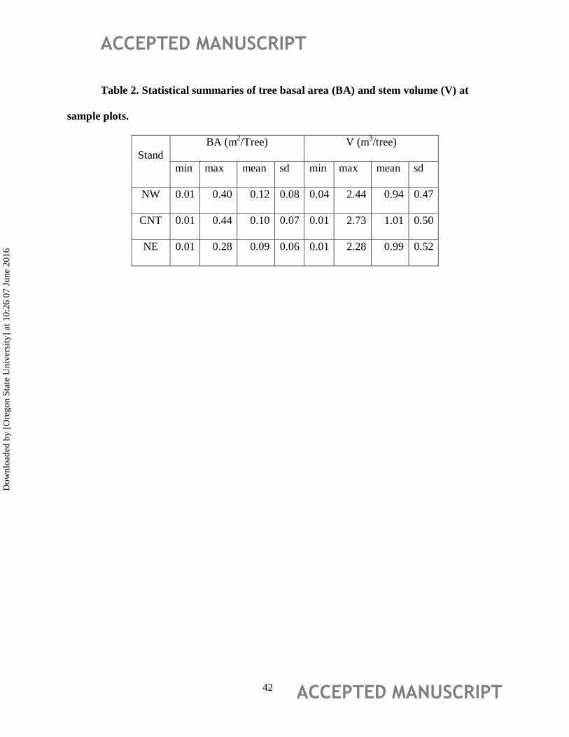
ACCEPTED MANUSCRIPT

ACCEPTED MANUSCRIPT 42

Table 2. Statistical summaries of tree basal area (BA) and stem volume (V) at

sample plots.

Stand

BA (m2/Tree) V (m

3/tree)

min max mean sd min max mean sd

NW 0.01 0.40 0.12 0.08 0.04 2.44 0.94 0.47

CNT 0.01 0.44 0.10 0.07 0.01 2.73 1.01 0.50

NE 0.01 0.28 0.09 0.06 0.01 2.28 0.99 0.52

Dow

nloa

ded

by [

Ore

gon

Stat

e U

nive

rsity

] at

10:

26 0

7 Ju

ne 2

016

ACCEPTED MANUSCRIPT

ACCEPTED MANUSCRIPT 43

Table 3. LiDAR flight parameters

LIDAR Survey Parameters

Scan Frequency 45 Hz

Scan Angle +/- 20 deg

Scan Cutoff +/- 4.0 deg

Scan Offset 0 deg

System PRF 125 kHz

Swath Width 344.64 m

Flying Altitude 600m AGL

Down Track Resolution 0.75 m

Points per square meter 5.06

Horizontal Datum NAD83

Vertical Datum NAVD88 (GEOID 03)

Projection UTM Zone 16N

Dow

nloa

ded

by [

Ore

gon

Stat

e U

nive

rsity

] at

10:

26 0

7 Ju

ne 2

016

ACCEPTED MANUSCRIPT

ACCEPTED MANUSCRIPT 44

Table 4. Individual tree detection in the test subplots. The highlighted gray color

represents the best results, which were determined by comparing the number of trees detected

(NTD) to the field-based tree inventory number (N). The closest values of NTD compared with

N were selected as the best results.

Plots Stand COV Ref.

(N)

TWS

3x3 5x5 7x7

SWS SWS SWS

NF 3x3 5x5 NF 3x3 5x5 NF 3x3 5x5

1 NW 68.39 803 4675 1112 587 1246 702 478 620 507 413

2 75.63 815 4725 1156 586 1312 674 480 639 514 410

3 CNT 70.40 519 4063 893 467 1028 515 393 485 399 340

4 70.96 503 4346 939 490 1079 548 410 526 425 370

5 71.47 572 4256 1021 536 1131 632 437 570 467 381

6 72.62 543 4208 953 505 1096 584 426 550 440 385

7 73.17 777 4222 1052 577 1110 622 449 552 452 383

8 75.53 621 4723 1050 573 1221 620 465 609 483 410

9 NE 60.13 321 2994 684 346 750 373 272 344 275 243

10 61.75 306 3222 701 363 771 414 283 374 300 250

11 63.85 366 3366 750 393 852 427 319 414 323 292

12 63.96 338 3319 743 370 849 396 292 411 318 265

Dow

nloa

ded

by [

Ore

gon

Stat

e U

nive

rsity

] at

10:

26 0

7 Ju

ne 2

016

ACCEPTED MANUSCRIPT

ACCEPTED MANUSCRIPT 45

13 72.24 737 4006 940 510 1018 563 405 521 436 368

14 74.50 810 4379 1012 547 1119 612 437 530 463 385

15 75.56 797 4357 1023 561 1145 620 452 567 454 391

Ref.: reference number of tree per test plot (N); TWS: fixed treetop windows size; SWS:

fixed smoothing windows size; NF: no filter applied; NE: Northeast stand; CNT: Central stand

and NW: Northwest stand.

Dow

nloa

ded

by [

Ore

gon

Stat

e U

nive

rsity

] at

10:

26 0

7 Ju

ne 2

016

ACCEPTED MANUSCRIPT

ACCEPTED MANUSCRIPT 46

Table 5. Accuracy assessment results of LiDAR-based individual tree detection

according to recall (r), precision (p) and F-score (F) statistics parameters.

Subplots COV (%)

Number of Trees Detected (NTD)

r p F

LiDAR Reference FP FN TP

1 46.21 13 16 1 4 12 0.75 0.92 0.83

2 46.87 16 18 2 4 14 0.78 0.88 0.82

3 50.66 8 6 2 0 6 1.00 0.75 0.86

4 56.55 5 5 0 0 5 1.00 1.00 1.00

5 60.31 4 4 0 0 4 1.00 1.00 1.00

6 63.02 4 4 0 0 4 1.00 1.00 1.00

7 64.71 9 8 1 0 8 1.00 0.89 0.94

8 67.13 7 5 2 0 5 1.00 0.71 0.83

9 71.41 16 17 3 4 13 0.76 0.81 0.79

10 71.45 18 21 2 5 16 0.76 0.89 0.82

11 74.33 20 23 4 7 16 0.70 0.80 0.74

12 76.93 11 10 2 1 9 0.90 0.82 0.86

13 80.56 23 27 3 7 20 0.74 0.87 0.80

14 85.58 15 13 3 1 12 0.92 0.80 0.86

15 83.48 8 8 1 1 7 0.88 0.88 0.88

Overall 66.41 177 185 26 34 151 0.82 0.85 0.83

Dow

nloa

ded

by [

Ore

gon

Stat

e U

nive

rsity

] at

10:

26 0

7 Ju

ne 2

016

ACCEPTED MANUSCRIPT

ACCEPTED MANUSCRIPT 47

Table 6. Accuracy assessment results for the individual tree detection as a function of

LiDAR-derived COV. FP: False positive; FN: False negative; TP: True positive; r: recall; p:

precision and F: F-score.

COV (%)

Number of Trees Detected (NTD)

r p F

LiDAR Reference FP FN TP

≤ 70 60 53 9 (17.0) 2 (3.8) 51 (96.2) 0.96 0.85 0.90

>70 117 132 17 (12.9) 32 (24.2) 100 (75.8) 0.76 0.85 0.80

Overall 177 185 26 (14.1) 34 (18.1) 151 (81.6) 0.82 0.85 0.83

Dow

nloa

ded

by [

Ore

gon

Stat

e U

nive

rsity

] at

10:

26 0

7 Ju

ne 2

016

ACCEPTED MANUSCRIPT

ACCEPTED MANUSCRIPT 48

Table 7. Estimated tree attributes summarized at the stand-level.

Stands NTD

Ht (m) BA (m2) V (m

3)

Mean Sd Mean Sd Total Mean Sd Total

NW 36958 23.17 4.14 0.10 0.07 3824.11 0.96 0.40 35658.33

CNT 52184 21.26 5.34 0.09 0.07 4478.04 0.80 0.49 42114.29

NE 35980 21.10 5.42 0.09 0.07 3119.95 0.79 0.49 28564.40

NTD=Number of Trees Detected

Dow

nloa

ded

by [

Ore

gon

Stat

e U

nive

rsity

] at

10:

26 0

7 Ju

ne 2

016

ACCEPTED MANUSCRIPT

ACCEPTED MANUSCRIPT 49

Figure 1. Longleaf pine forest location A, B and D and profile picture, at Ichauway in

southwestern Georgia, USA. NW: Northwest ; CNT: central and NE: Northeast stands.

Dow

nloa

ded

by [

Ore

gon

Stat

e U

nive

rsity

] at

10:

26 0

7 Ju

ne 2

016

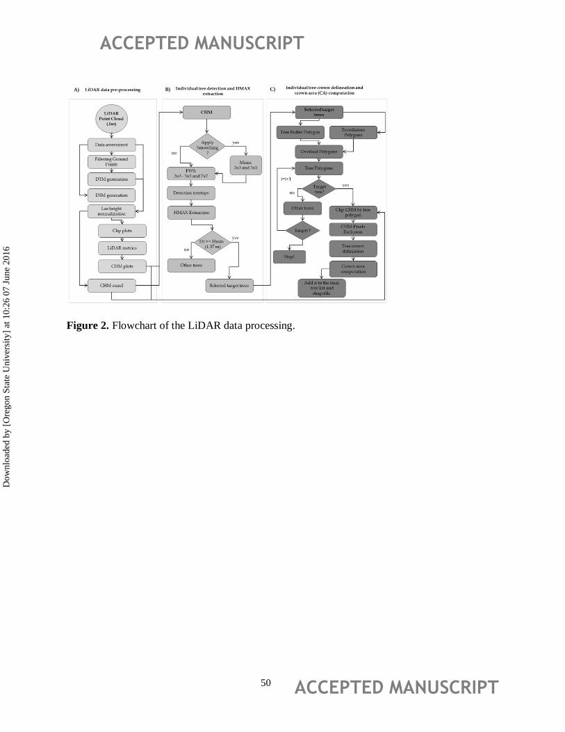
ACCEPTED MANUSCRIPT

ACCEPTED MANUSCRIPT 50

Figure 2. Flowchart of the LiDAR data processing.

Dow

nloa

ded

by [

Ore

gon

Stat

e U

nive

rsity

] at

10:

26 0

7 Ju

ne 2

016

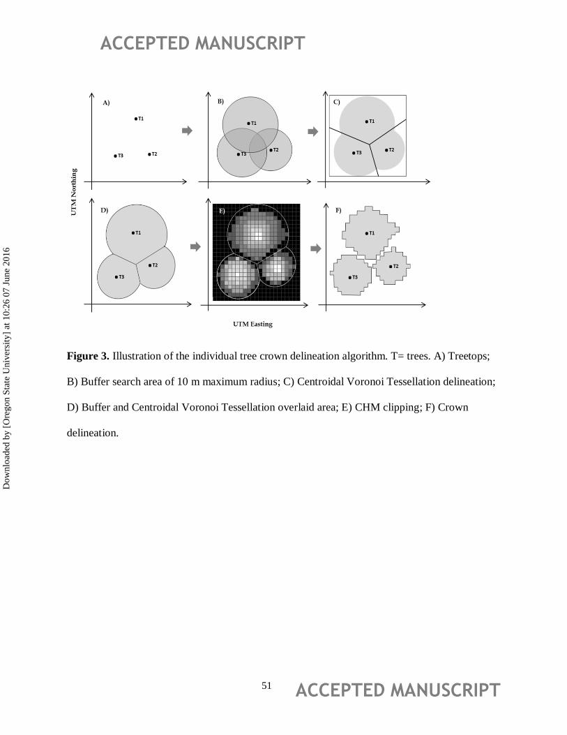
ACCEPTED MANUSCRIPT

ACCEPTED MANUSCRIPT 51

Figure 3. Illustration of the individual tree crown delineation algorithm. T= trees. A) Treetops;

B) Buffer search area of 10 m maximum radius; C) Centroidal Voronoi Tessellation delineation;

D) Buffer and Centroidal Voronoi Tessellation overlaid area; E) CHM clipping; F) Crown

delineation.

Dow

nloa

ded

by [

Ore

gon

Stat

e U

nive

rsity

] at

10:

26 0

7 Ju

ne 2

016

ACCEPTED MANUSCRIPT

ACCEPTED MANUSCRIPT 52

Figure 4. rSTree algorithm: searching for the LiDAR and reference trees. MED= maximum

Euclidian distance, MHD= minimum height deference, HD= height difference.

Dow

nloa

ded

by [

Ore

gon

Stat

e U

nive

rsity

] at

10:

26 0

7 Ju

ne 2

016

ACCEPTED MANUSCRIPT

ACCEPTED MANUSCRIPT 53

Figure 5. LiDAR based plot HMAX (A) and COV( B); and tree density(C) measured in the field

at the longleaf pine test plots. Error bars indicate standard deviations.

Dow

nloa

ded

by [

Ore

gon

Stat

e U

nive

rsity

] at

10:

26 0

7 Ju

ne 2

016

ACCEPTED MANUSCRIPT

ACCEPTED MANUSCRIPT 54

Figure 6. LiDAR-derived COV versus number of reference trees (N) measured in the field (A),

and LiDAR-derived versus reference tree densities.

Dow

nloa

ded

by [

Ore

gon

Stat

e U

nive

rsity

] at

10:

26 0

7 Ju

ne 2

016

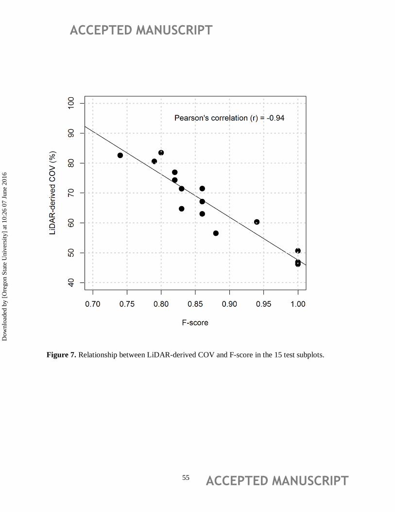
ACCEPTED MANUSCRIPT

ACCEPTED MANUSCRIPT 55

Figure 7. Relationship between LiDAR-derived COV and F-score in the 15 test subplots.

Dow

nloa

ded

by [

Ore

gon

Stat

e U

nive

rsity

] at

10:

26 0

7 Ju

ne 2

016

ACCEPTED MANUSCRIPT

ACCEPTED MANUSCRIPT 56

Figure 8. Distribution of LiDAR-derived HMAX (A) and CA (B) values. The black line

represented a fitted distribution.

Dow

nloa

ded

by [

Ore

gon

Stat

e U

nive

rsity

] at

10:

26 0

7 Ju

ne 2

016

ACCEPTED MANUSCRIPT

ACCEPTED MANUSCRIPT 57

Figure 9. Equivalence test graphs for the imputed and observed longleaf pine tree attributes. A)

Tree Height Ht (m); B) Tree Basal Area - BA (m2); Tree Volume - V (m3), N=1061. The

equivalence plots design presented herein are an adaptation of the original equivalence plots

presented by Robinson (2015). The grey polygon represents the ± 25% region of equivalence for

the intercept, and the red vertical bar represents a 95% of confidence interval for the intercept.

The imputed tree attributes are equivalent to the reference attributes when the red bar is

completely within the grey polygon. If the grey polygon is lower than the red vertical bar, the

imputed attributes are biased low; if it is higher than the red vertical bar, the imputed forest

attributes are biased high. The grey dashed line represents the ± 25% region of equivalence for

the slope, and the red vertical bar is contained completely within the grey dashed line, the

pairwise measurements are equal. A bar that is wider than the region outlined by the grey dashed

lines indicates highly variable predictions. The gray dots are the pairwise measurements, and the

solid line is a best-fit linear model for the pairwise measurements. The black dashed line

represents the 1:1 line.

Dow

nloa

ded

by [

Ore

gon

Stat

e U

nive

rsity

] at

10:

26 0

7 Ju

ne 2

016

ACCEPTED MANUSCRIPT

ACCEPTED MANUSCRIPT 58

Figure 10. Imputed and observed tree attributes distribution from the testing dataset. A, B and C

represent Ht, BA and V distribution across the three stands. The numbers 1 and 2 represent the

imputed and observed values. The black line represented a fitted distribution and the dashed

vertical line represented the mean.

Dow

nloa

ded

by [

Ore

gon

Stat

e U

nive

rsity

] at

10:

26 0

7 Ju

ne 2

016

ACCEPTED MANUSCRIPT

ACCEPTED MANUSCRIPT 59

Figure 11. Distribution of imputed tree attributes (Ht, BA and V) across the three stands in the

study area. The numbers from 1 to 3 represent the attributes Ht, BA and V, respectively. The

letters from A to D represent the NE, CNT and NW, and all stands, respectively. The black line

represented a fitted distribution and the dashed vertical line represented the mean.

Dow

nloa

ded

by [

Ore

gon

Stat

e U

nive

rsity

] at

10:

26 0

7 Ju

ne 2

016

ACCEPTED MANUSCRIPT

ACCEPTED MANUSCRIPT 60

Figure 12. Illustration of individual tree detection and crown delineation under different COV

conditions. 1) COV = 90.96%; COV= 76.79%, and 3) COV= 58.66%. A) 2D visualization of the

tree location and crown delineation over the CHM. B) 3D visualization of the LiDAR point

cloud and reference trees measured in the field. C) 3D visualization of the LiDAR virtual forest,

and the reference tree locations.

Dow

nloa

ded

by [

Ore

gon

Stat

e U

nive

rsity

] at

10:

26 0

7 Ju

ne 2

016