![A MULTI-OBJECTIVE OPTIMIZATION APPROACH FOR DESIGNING AUTOMATED WAREHOUSES … · 2012-05-09 · controlling warehouses has been presented by Rouwenhorst et al. [8] in the form of](https://static.fdocuments.us/doc/165x107/5e8dbaf48ac5b24c3b455a96/a-multi-objective-optimization-approach-for-designing-automated-warehouses-2012-05-09.jpg)
Pallets and Warehouses Optimization
32
A Case Study of Joint Online Truck Scheduling and Inventory Management for Multiple Warehouses ∗ C. Helmberg † S. R¨ ohl ‡ January 2005, revised April 2006, July 2006 Abstract For a real world problem – transporting pallets between warehouses in order to guarantee sufficient supply for known and additional stochastic demand – we propose a solution approach via convex relaxation of an integer programming formulation, sui table for online optimizat ion. The essential new elemen t linkin g routing and inventory management is a convex piecewise linear cost function that is based on minimi zing the expected number of palle ts that still need transportati on. For speed, the con ve x rel axa tion is sol ved appr ox imately by a bundle approac h yie lding an online schedule in 5 to 12 min ute s for up to 3 wareho use s and 40000 artic les; in contrast, computation times of state of the art LP-solvers are prohibitive for online applic ation. In extensi ve nume rical experimen ts on a real world data stream, the approximat e soluti ons exhibit negligible loss in quality; in long term simulations the proposed method reduces the average number of pallets needing transportation due to short term demand to less than half the number observed in the data stream. Keywords: conv ex relaxati on, integer programmi ng, stochastic demand, netw ork models, large scale problems, bundle method, logistics, vehicle routing MSC 2000: 90B06; 90C06, 90C90, 90B05 1 In tr oduc ti on Consider a company operating several warehouses, each having a master automatic storage system (MASS) that holds stock on pallets. Here, a pallet is a wooden platform on which typically a large quantity of only one article is piled up and which is suitable for automatic transportation by conve yo r belts and sta cker cranes. The warehous es are linked by a shuttl e service of sev eral truc ks for transport ing pall ets from one MASS to another. A common online data stream reports the movement of stock in all warehouses as well as the current pres ch eduled demand of today per warehouse. For certain reasons, demand scheduling cannot take into account the distribution of stock in the various MASSes. The central task is to provide, online, a schedule for transporting pallets between the MASSes ∗ This work was supported by research grant 03HEM2B4 of the German Federal Ministry of Education and Research. Responsibility for the content rests with the authors. † Fakult¨ at f¨ ur Mathemati k, T ec hni sc he Uni ve rsi t¨ at Chemnitz, D-09107 Chemni tz, Ge rman y , [email protected] ‡ V ora rlbe rg Universi ty of App lie d Sci ences, Hoc hsc hulst r. 1, A-6 850 Dor nbirn, Aus tria, ste- [email protected] 1
-
Upload
vladimir-trifunovic -
Category
Documents
-
view
224 -
download
0
Transcript of Pallets and Warehouses Optimization
8/3/2019 Pallets and Warehouses Optimization
http://slidepdf.com/reader/full/pallets-and-warehouses-optimization 1/32
A Case Study of Joint Online Truck Scheduling and
Inventory Management for Multiple Warehouses∗
C. Helmberg† S. Rohl‡
January 2005, revised April 2006, July 2006
Abstract
For a real world problem – transporting pallets between warehouses in order toguarantee sufficient supply for known and additional stochastic demand – we proposea solution approach via convex relaxation of an integer programming formulation,suitable for online optimization. The essential new element linking routing andinventory management is a convex piecewise linear cost function that is based on
minimizing the expected number of pallets that still need transportation. For speed,the convex relaxation is solved approximately by a bundle approach yielding anonline schedule in 5 to 12 minutes for up to 3 warehouses and 40000 articles; incontrast, computation times of state of the art LP-solvers are prohibitive for onlineapplication. In extensive numerical experiments on a real world data stream, theapproximate solutions exhibit negligible loss in quality; in long term simulations theproposed method reduces the average number of pallets needing transportation dueto short term demand to less than half the number observed in the data stream.
Keywords: convex relaxation, integer programming, stochastic demand, networkmodels, large scale problems, bundle method, logistics, vehicle routing
MSC 2000: 90B06; 90C06, 90C90, 90B05
1 Introduction
Consider a company operating several warehouses, each having a master automatic storagesystem (MASS) that holds stock on pallets. Here, a pallet is a wooden platform on whichtypically a large quantity of only one article is piled up and which is suitable for automatictransportation by conveyor belts and stacker cranes. The warehouses are linked by ashuttle service of several trucks for transporting pallets from one MASS to another. Acommon online data stream reports the movement of stock in all warehouses as well asthe current prescheduled demand of today per warehouse. For certain reasons, demandscheduling cannot take into account the distribution of stock in the various MASSes. Thecentral task is to provide, online, a schedule for transporting pallets between the MASSes
∗This work was supported by research grant 03HEM2B4 of the German Federal Ministry of Educationand Research. Responsibility for the content rests with the authors.
†Fakultat fur Mathematik, Technische Universitat Chemnitz, D-09107 Chemnitz, Germany,[email protected]
‡Vorarlberg University of Applied Sciences, Hochschulstr. 1, A-6850 Dornbirn, Austria, [email protected]
1

8/3/2019 Pallets and Warehouses Optimization
http://slidepdf.com/reader/full/pallets-and-warehouses-optimization 2/32
by means of the trucks, so that all articles are available at the right warehouse in time tosatisfy current demand. The key to success will be to exploit free capacity on the trucksin order to satisfy expected future demand that must be estimated from past demand.
We suggest a solution approach based on convex relaxation and demonstrate its practi-cal suitability on real world data of our industrial partner eCom Logistik GmbH & Co. KG.For up to three warehouses and roughly 40000 articles the method computes a schedulewithin five to twelve minutes. In long term simulations it reduces the average number of pallets that have to be transported on short notice due to demand to less than half thenumber of the current semi-automatic approach. A similar approach to the one devel-oped here should be applicable whenever an automatic supply management system needsto redistribute supply containers according to online demand among several sub storagesystems in the presence of some transportation bottle neck like elevators, stacker cranesor automatic guided vehicles.
Several issues are of relevance in this problem: an appropriate stochastic optimizationmodel is required that links the success probability of the inventory of the warehouses
to the truck rides; the model must be solvable within short time in order to be suitablefor online computations; the approach must be sufficiently robust to compensate frequentexternal changes in orders and uncertainties of the logistic transportation process.
In our method we follow the classical approach to model large scale transportation ornetwork design problems as multicommodity flow problems (see e.g. [23, 20, 18]). Thesecan be decomposed and solved efficiently via Lagrangian relaxation by combining min-costflow algorithms (see e.g. [1]) and bundle methods (see e.g. [14, 6]). In particular, we modelthe rides of the trucks as well as the flow of pallets between warehouses by time discretizednetworks coupled via linear capacity constraints. Our main contribution is probably thedevelopment of a convex piecewise linear cost function, that models the stochastic quality
of the warehouse configurations. Its primary aim is to minimize the expected number of pallets that have yet to be transported. Due to its favorable structure, even moderatelyaccurate solutions seem to give rise to reasonable schedules. This allows the use of theaforementioned fast approximate solvers suitable for online optimization. The approachmakes no assumptions on what part of the suggested solution has been accepted by thehuman dispatcher but relies exclusively on the current system status described by an onlinestream of status messages. This seems to be vital in view of severe logistic uncertainties.
There is a vast literature on inventory management and logistics (see e.g. [9]), yetwe found very few references that deal with both problems at the same time; none of them, however, treat both problems in sufficient detail for our purposes. In some worksthe transportation process is assumed to be instantaneous (see e.g. [16, 17, 7, 3, 27]), inothers the stochastic part is fixed (see e.g. [2, 8]) or considerations are reduced to onlyone product [21]. To the best of our knowledge the approach proposed here is the firstthat deals jointly with inventory management of multiple products and inter warehouselogistics involving vehicle routing with transportation times.
Dealing with uncertainties in the data is currently a very active area of research, thetwo main branches being stochastic programming and convex robust optimization. Integerstochastic programming, which would be required here, concentrates on modeling uncer-tainties by scenario trees (see e.g. [22, 24, 28]); due to the quick growth of these trees,
2
8/3/2019 Pallets and Warehouses Optimization
http://slidepdf.com/reader/full/pallets-and-warehouses-optimization 3/32
practical examples seem to deal with no more than ten dimensional probability distribu-tions. Considering the size of our probability space this approach is currently impractical,in particular in view of the online requirements. Convex robust optimization asks for anoptimal solution subject to feasibility for all choices of the uncertain parameters specifiedvia predefined convex sets (see e.g. [4]). This approach might help to ensure the avail-ability of a minimum amount of stock if there is sufficient time and storage capacity. Inthe absence of the latter two, however, the approach may even be counterproductive dueto its lack of ability to discern between infeasible instances. In fact, most instances of our application already contain some unsatisfiable requirements which may be resolvedby postponing a few orders in the schedule. Stochastic measures seem to be much bettersuited for these purposes.
The content is structured as follows. Section 2 gives the necessary background on thereal world problem. Next we present our optimization model in two steps: in Section 3we formulate the set of feasible solutions by introducing the networks, variables, and con-straints; Section 4 is devoted to the cost function. Implementational aspects such as the
generation of distribution data, the approach for solving the relaxation, and the roundingheuristic are described in Section 5. Extensive computational results on the real worlddata stream of our industrial partner are presented in Section 6; these include compar-ative runs with exact solution methods and a simulation run over 100 days for two andthree warehouses. Finally, we offer some conclusions and outline possible enhancementsin Section 7.
2 Problem Description
The usual conception of a demand problem in logistics as laid out in the first paragraph
of the introduction is that there is complete knowledge of current stock, full control overthe logistic process and that uncertainties are confined to future demand. In practice,however, significant uncertainties are present in almost every logistic aspect and have tobe taken care of. We will not be able to model all uncertainties to our satisfaction, but allof them had a strong impact on our modeling decisions. In order to share the obstaclesmet in practice as well as to motivate our decisions we present a rather detailed descriptionof the actual problem.
Demand Structure. Our industrial partner, eCom Logistik GmbH & Co. KG, op-erates several warehouses (initially there were three, meanwhile only two remained) indifferent locations within the same city and offers logistics services to business customers.
In particular, it stores the products of a business customer and processes orders addressedto the business customer by picking and packing the ordered items into boxes or on palletsand passing them on to a shipping agency that takes care of the final delivery to the correctaddress. E.g., a startup company selling via the Internet could contract eCom Logistik forstoring and delivering its products.
The business model implies important differences to standard inventory managementproblems. First, the task of our partner is to deliver, upon request, the goods storedbut it is not its responsibility that sufficient goods are within its store, so the standardscenario of “ordering problems” does not apply. Second, there is no information available
3
8/3/2019 Pallets and Warehouses Optimization
http://slidepdf.com/reader/full/pallets-and-warehouses-optimization 4/32
about the customers expectations on the development of demand. Therefore stochasticdemand forecasts must be based on past demand for a particular product alone. Thesupply shipments by the customer for replenishing the store seem to be unpredictable inthe sense that they are rare singular events of strongly varying size. In each shipmenta customer defined number of pallets is delivered to one of the warehouses. Each suchsupply pallet holds an, in general standardized, quantity of only one article and the entirepallet is stored automatically in the local MASS. Third and finally, at the logistic systemlevel, knowledge about the products of the business customers is restricted to an articleidentifier number (article ID) and – at best – to the number of items of this article to beexpected on a typical supply pallet.
Due to the structure of the customers (a major customer is the Herlitz PBS AG, alarge company producing stationery) a typical order is placed by small to medium sizedretailers and consists of a long list of assorted articles. Orders are accepted till noon,delivery of these orders starts at 2 pm and should be finished till 2 pm the next day.When such an order arrives, it is prescheduled to a certain warehouse and time slot for
picking. At this time, all the items on the list have to be available in the picking lines of the selected warehouse so that the entire order can be shipped in one unit. The pickinglines are replenished automatically or by local personnel by requesting a certain amountof the respective article from the central logistic system. This consists of a hierarchy of automatic storage systems linked by a network of conveyor belts. At the bottom level eachwarehouse runs a MASS that holds the pallets supplied by the business customers. Due tosize restrictions of the storage system or due to simultaneous demand at various locationsit is not always possible to hold pallets of each article in each MASS, so pallets have to beshipped between the warehouses on time and this is precisely the task addressed in thispaper.
The Logistic Process. Suppose now that a request triggers the retrieval of a palletcorresponding to a certain article from the local MASS and that several pallets are avail-able. Then one is selected by a local first-in-first-out (FIFO) strategy and delivered to anunpacking location where certain subquantities are removed from the pallet by hand. If,after this, the pallet is not empty it is reinserted into the MASS. In general, this is a oneway street and unpacked products do not reenter the MASS, unless a surplus amount inthe picking lines of one warehouse is desperately needed at another warehouse or the prod-uct is completely removed from the picking lines. Only on these occasions it may happenthat products are again packed onto pallets for the MASS. Such operations are avoidedbecause they are costly and not well supported by the logistic system. In consequence,almost all pallets in the MASS carry only one product and typically all except one holdthe initial amount provided by the business customer.
If supply needs to be brought in from the MASS of another warehouse, the centralstorage operating system is told to assign, at a given retrieval time, the desired destinationto a FIFO-selected pallet of that MASS; a pallet marked in this way will be called aprescheduled pallet . At the scheduled time, the pallets destination label is changed and anautonomous system of stacker cranes, conveyor belts and elevators moves the pallet into oneof two to five waiting lines with a joint capacity of roughly 40 pallets in front of two to threeautomatic loading platforms, each capable of loading a maximum of 27 pallets into a truck.
4
8/3/2019 Pallets and Warehouses Optimization
http://slidepdf.com/reader/full/pallets-and-warehouses-optimization 5/32
Congestions on the way to the platforms may lead to delays of more than half an hour; thearrival sequence needs not to correspond with scheduled retrieval times. It is not possible tomove “urgent” pallets to the front, so waiting lines should not be filled too early. Now andthen some authorized users, not involved in the truck scheduling process, may mark palletsfor transport and expect to be served promptly. These pallets appear as prescheduledpallets in the operating system and shortly thereafter at the waiting queues. The numberof pallets fitting on a truck depends on its capacity and, more importantly, on the widthof the pallets, which is a further source of uncertainties. Vibrations during automatictransportation may dearrange the packing on the pallets; increased space requirementsare detected by light barriers and updated automatically. Special oversized pallets maynot fit on all trucks (some have retaining walls in the middle) or may occupy large partsof the truck. Arrangement of the pallets on the loading platform and loading the truckis automatic, the expected number of pallets loaded on the biggest truck is about 24, thetime requirements here are well known and stable (roughly ten minutes), but the limitednumber of platforms leads to restrictions on the number of trucks that can be handled at
the same time. Left over pallets are kept in the waiting line and may block the way if the next truck serves a different direction. The driving time of trucks depends on currenttraffic. Automatic unloading and transportation into the destination MASS may again besubject to delays. Changing layout and design of the logistic system was not an option.
The current solution method used in practice for the task of scheduling pallets andtrucks is half automatic. Pallets are automatically put on a list if the available amountof an article falls short of a given minimum for this article. The minima are set by someautomatic rules and are controlled by a human dispatcher, who regularly initiates thetransportation of pallets for known short term demand and for pallets on this list.
The Input Data Stream. Together with our industrial partner a new data protocol
was developed for efficient online updating of the current ordering and inventory statusknown to the system software. The latter needs not reflect the true state of the system dueto the asynchronous nature of the underlying logistic system, i.e., certain bookings mayarrive significantly later, because they are entered by humans or because of communicationdelays between warehouses. Among others, the messages of the protocol give a completeonline account of
• article basics (including article ID and the standard amount of the article that is ona typical pallet; it may be zero if the data is not supplied by the customer),
• header information for orders (with prescheduled picking time and warehouse),
• delivery items per order (article ID and amount to deliver),
• picks (reports that [a part of] the amount of a delivery item has been fulfilled),
• stock movements (between real and/or virtual storage systems),
• prescheduled pallets (the information includes article ID with amount loaded, sched-uled retrieval time, and source and destination warehouses),
• pallets currently in transport (those having reached a loading platform),
• available truck capacities (per truck a time period when it is available and the ex-pected number of pallets it can load).
5
8/3/2019 Pallets and Warehouses Optimization
http://slidepdf.com/reader/full/pallets-and-warehouses-optimization 6/32
“Current” stock and demand can be updated efficiently with these messages. We also usethis data for generating demand distributions, see §5. Note, because of the business modelthere is certainly enough stock in the distributed storage system to cover the entire demand,even if the current figures show negative stock at single warehouses due to asynchronousbookings. Unfortunately, no information is available on the current position of the trucksor on the direction of their next ride.
The solution of the optimization process yields a suggestion for the dispatcher of thetrucks who will then fix a route and select particular pallets for transportation. Dependingon possible additional oral information not available in the operating system, the dispatchermay or may not follow the suggestions. The only feedback on these decisions are newmessages announcing prescheduled pallets.
Goals for the Cost Function. For acceptance as well as practical reasons we haveagreed with our industrial partners on a rather strict priority order for the sequence inwhich pallets should be transported by the trucks.
Priority Level 1: Prescheduled pallets should be served as quickly as possible after theirretrieval time. They have been requested by the truck dispatcher or an authorizeduser, presumably for a good reason. They will appear at the waiting queues at thattime and if they are not transported, they will likely block the way of other pallets.
Priority Level 2: Pallets that are needed to cover the known demand of the next six daysshould be transported in the sequence of their due dates.
Priority Level 3: If there is still room on the trucks, further pallets may be transportedfor supply management based on demand forecasts. Among these, the priority ordershould reflect the estimated probability that the pallet is needed within the next
three days, say.While priority level 1 is well motivated, there are, in our view, several attractive alterna-tives for replacing the rather strict priority rules 2 and 3 that might well be worth pursuing.A strong motivation for our industrial partner to prefer level 2 to level 3 seemed to be thatit is easier to defend transportation decisions against external criticism if they are basedon factual rather than on estimated demand. Long term improvement, however, dependson the choice of level 3 pallets.
No actual costs are known for delays in transportation or for the violation of duedates. For inventory management purposes, stochastic models often assume a certainamount of available space and ask for the best use of this space in a probabilistic sense.
It was the explicit wish of our industrial partner not to use such a concept, because theamount of available space is itself a highly uncertain parameter in an asynchronous logisticenvironment and depends on several other factors (e.g. depending on the width or heightof a pallet there may be room in the automatic storage system or not; also, upon needthe dispatcher may open up some intermediate storage facilities). Therefore, they saw nopossibility to provide the amount of free storage space automatically. Rather it was agreedthat the amount of pallets transported for stock-keeping purposes should be controlled viaan “upper probability level” π ∈ (0, 1) measuring the probability that available stock of an article at a warehouse suffices for a given period of days with respect to an appropriate
6

8/3/2019 Pallets and Warehouses Optimization
http://slidepdf.com/reader/full/pallets-and-warehouses-optimization 7/32
stochastic model of demand. If stock exceeds the upper level π, no further pallets shouldbe brought in for this article. Furthermore an upper limit was imposed on the amount of pallets transported to each warehouse for stock building purposes. Without informationon available storage it is difficult to make room by removing superfluous articles, andindeed our industrial partner did not wish to shift stock for such purposes without humaninitiative. We might add that our current approach could easily be extended to such tasksif appropriate information is provided.
We do not know how to model the problem of left over pallets due to queuing andpacking problems directly. Instead, we hope that by planning with respect to the expectedcapacity of the trucks, most of these problems cancel out over time. If not, left over palletswill again appear as prescheduled pallets in the next planning process and will then betaken care of. Most other logistic uncertainties concern transportation times betweenMASS and loading platforms as well as driving times of the trucks and will be compensatedby using sufficiently large overestimates. The model will, however, include the constraintson the number of loading platforms as well as the restrictions on the number of pallets
transported for stock keeping purposes.
3 Optimization Model, Part I: The Feasible Set
For modeling the route of trucks and the movement of pallets, we use the standard approachof time discretized network flows coupled by linear constraints. Most of this is canonical,so the description is kept rather short and neglects some aspects of minor importance. Fora detailed account, see the preprint [13].
We assume the time discretization to be given (in minutes) as a finite sequence of nonnegative integers 0 ≤ t1 < · · · < tnT
, nT ∈ N and set T = {ti : 1 ≤ i ≤ nT } (in
our implementation, the time span of one day is discretized into steps of 10 minutes). Wedenote the set of warehouses at different locations by W . To allow for a separate truckdepot d /∈ W we set W d = W ∪ {d}. The set of different products (articles) is denotedby P . We collect all trucks that have not to be discerned (e.g. in terms of capacity orcompatibility with certain products) in truck classes and collect all truck classes in a set R.
The network structure will be described by directed multigraphs Dh = (V h, Ah) forsome index h with node set V h ⊂ W d × {A,B,C,L,U } × T and a multiset of arcs Ah
consisting of ordered pairs of nodes. For each node v ∈ V h, its three components willbe referred to by vW , vN , and vT ; the letter vN serves as a name to distinguish betweennodes referring to the same warehouse vW and time vT (see below). There will be no need
to discern parallel arcs explicitly, so we simply denote arcs by (v, w). Balances will bespecified via a vector bh ∈ Z
V h and lower and upper bounds by means of vectors lh ∈ ZAh
and uh ∈ (Z∪{∞})Ah. If not specified explicitly, balances and lower bounds are set to zeroand upper bounds to ∞. We will describe, in this sequence, truck graphs modeling therouting of trucks, article graphs for scheduling new pallets for transport, graphs for dealingwith prescheduled pallets, and finally the variables and coupling constraint between them.
Truck Graphs. The basic structure of these graphs is depicted in Figure 1 and foreach class of trucks r ∈ R it differs only due to driving speed or loading and unloadingproperties. The node set V r of the graph Dr = (V r, Ar) includes, for each time step t ∈ T
7
8/3/2019 Pallets and Warehouses Optimization
http://slidepdf.com/reader/full/pallets-and-warehouses-optimization 8/32
c u
l
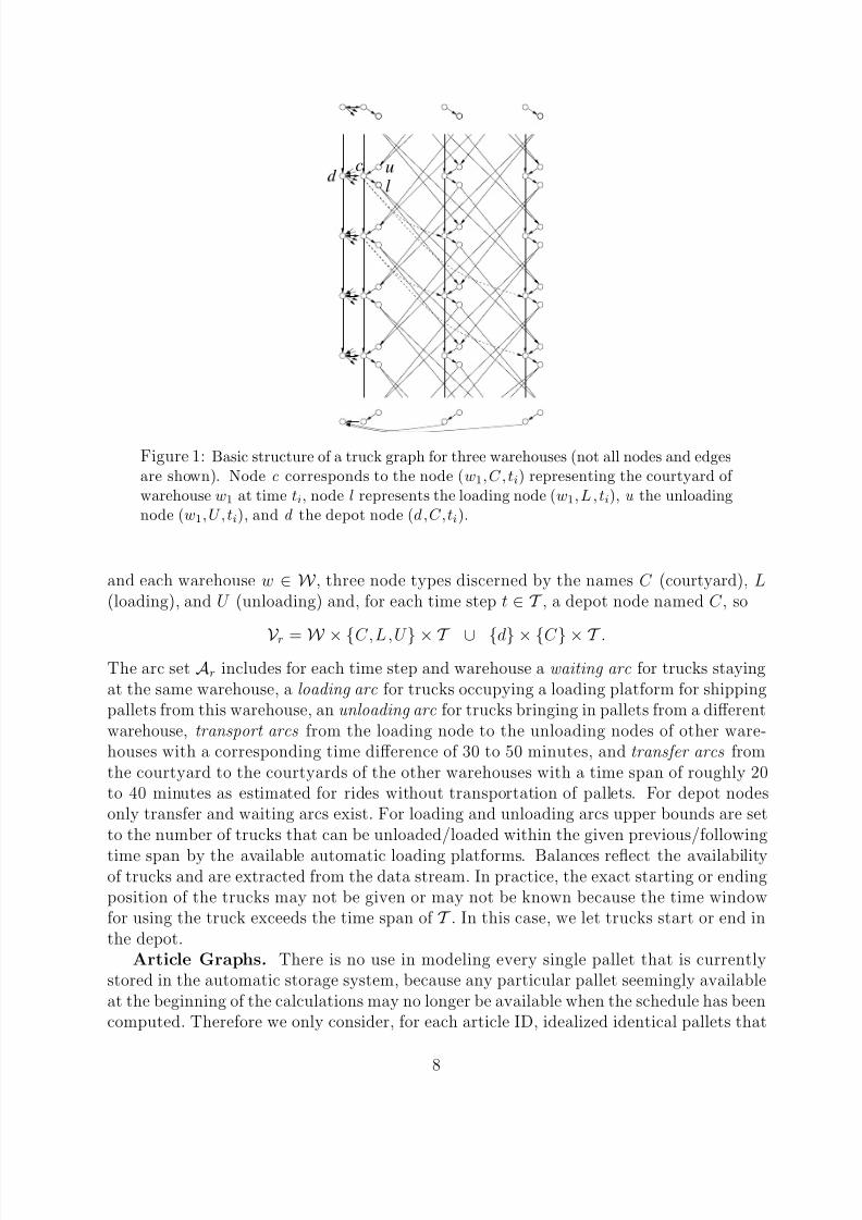
Figure 1: Basic structure of a truck graph for three warehouses (not all nodes and edgesare shown). Node c corresponds to the node (w1,C,ti) representing the courtyard of warehouse w1 at time ti, node l represents the loading node (w1,L,ti), u the unloadingnode (w1,U ,ti), and d the depot node (d,C,ti).
and each warehouse w ∈ W , three node types discerned by the names C (courtyard), L(loading), and U (unloading) and, for each time step t ∈ T , a depot node named C , so
V r = W × {C,L,U } × T ∪ {d} × {C } × T .The arc set Ar includes for each time step and warehouse a waiting arc for trucks stayingat the same warehouse, a loading arc for trucks occupying a loading platform for shippingpallets from this warehouse, an unloading arc for trucks bringing in pallets from a differentwarehouse, transport arcs from the loading node to the unloading nodes of other ware-houses with a corresponding time difference of 30 to 50 minutes, and transfer arcs fromthe courtyard to the courtyards of the other warehouses with a time span of roughly 20to 40 minutes as estimated for rides without transportation of pallets. For depot nodesonly transfer and waiting arcs exist. For loading and unloading arcs upper bounds are setto the number of trucks that can be unloaded/loaded within the given previous/following
time span by the available automatic loading platforms. Balances reflect the availabilityof trucks and are extracted from the data stream. In practice, the exact starting or endingposition of the trucks may not be given or may not be known because the time windowfor using the truck exceeds the time span of T . In this case, we let trucks start or end inthe depot.
Article Graphs. There is no use in modeling every single pallet that is currentlystored in the automatic storage system, because any particular pallet seemingly availableat the beginning of the calculations may no longer be available when the schedule has beencomputed. Therefore we only consider, for each article ID, idealized identical pallets that
8

8/3/2019 Pallets and Warehouses Optimization
http://slidepdf.com/reader/full/pallets-and-warehouses-optimization 9/32
ab
c
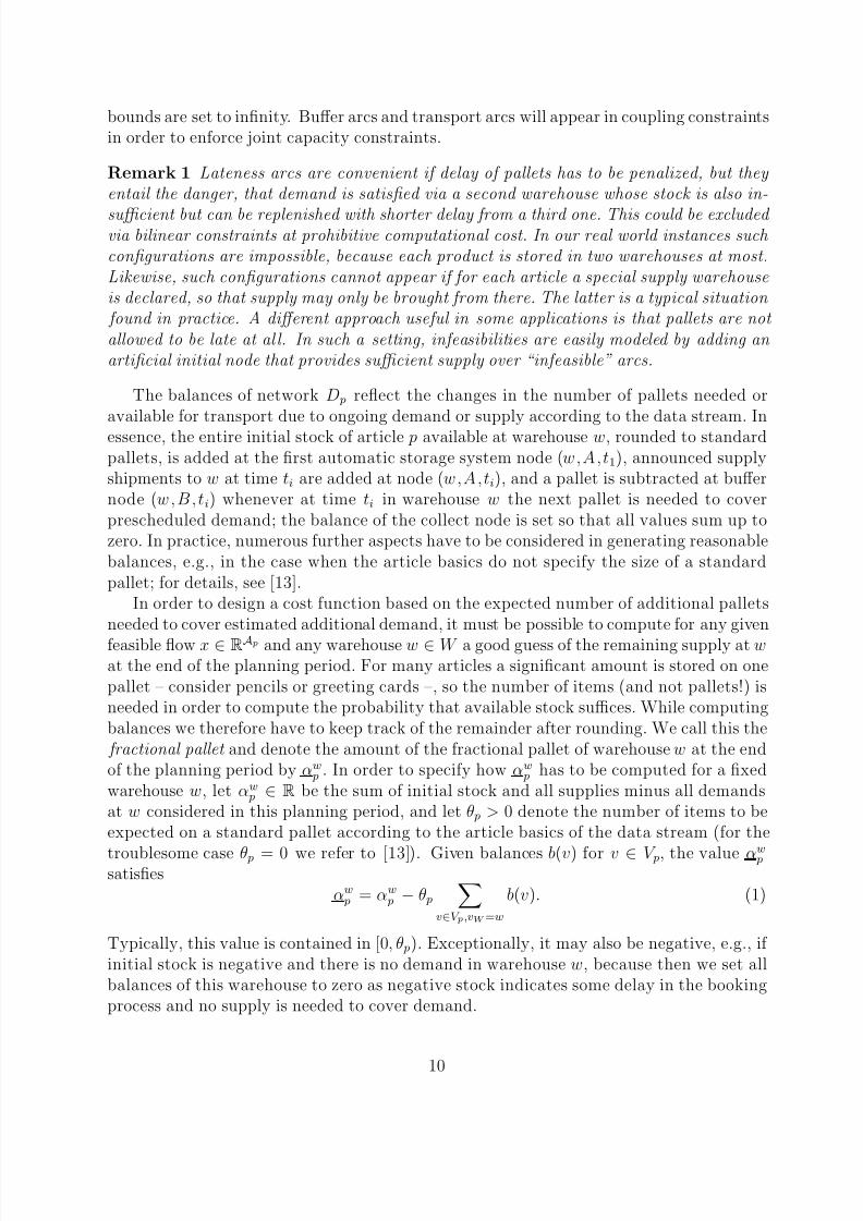
Figure 2: Basic structure of an article graph for three warehouses (not all nodesand edges are shown). Node a corresponds to the node (w1,A,t1) representing theautomatic storage system of warehouse w1 at time t1, node b represents the buffer node(w1,B , t1), and c the collect node (d,C,tnT
).
carry the amount promised by the article basics (and a single pallet carrying the entirestock of one warehouse if no such data is available). An attractive alternative would be tocompute a statistically representative amount from previous pallet data. Our industrial
partner, however, strongly preferred to rely on the given article basics that are within theresponsibility of the customer. So for each article p ∈ P the stock at each warehouseis discretized to standard pallets and there is one network per article p that models themovement of these pallets. The basic graph structure is sketched in Figure 2. Let p ∈ P befixed. The node set V p of the graph D p = (V p, A p) contains, for each time step t ∈ T andeach warehouse w ∈ W , two nodes discerned by the names A (automatic storage system)and B (transportation buffer), and one artificial node named (d,C,tnT
) (collect),
V p = W × {A, B} × T ∪ {(d,C,tnT )}.
The arc set A p includes for each time step and warehouse a storage arc for keeping pallets
inside the automatic storage system, a release arc for removing pallets from the automaticstorage system, a buffer arc that keeps pallets inside the transportation buffer, a latenessarc backwards in time for satisfying excess demand using future arrivals, and severaltransport arcs that allow pallets to be shipped from the local buffer to the buffer of otherwarehouses. Each transport arc corresponds to a particular transport arc in some truckgraph Dr; its time span is considerably longer and includes about 60 minutes preparationtime before loading and the same time span after unloading. Finally, collect arcs andinfeasible arcs connect the collect node to the last time step of each warehouse and allowto compensate excess demand in one warehouse by stock in another warehouse. All upper
9
8/3/2019 Pallets and Warehouses Optimization
http://slidepdf.com/reader/full/pallets-and-warehouses-optimization 10/32
bounds are set to infinity. Buffer arcs and transport arcs will appear in coupling constraintsin order to enforce joint capacity constraints.
Remark 1 Lateness arcs are convenient if delay of pallets has to be penalized, but they entail the danger, that demand is satisfied via a second warehouse whose stock is also in-
sufficient but can be replenished with shorter delay from a third one. This could be excluded via bilinear constraints at prohibitive computational cost. In our real world instances such configurations are impossible, because each product is stored in two warehouses at most.Likewise, such configurations cannot appear if for each article a special supply warehouseis declared, so that supply may only be brought from there. The latter is a typical situation found in practice. A different approach useful in some applications is that pallets are not allowed to be late at al l. In such a setting, infeasibilities are easily modeled by adding an artificial initial node that provides sufficient supply over “infeasible” arcs.
The balances of network D p reflect the changes in the number of pallets needed oravailable for transport due to ongoing demand or supply according to the data stream. Inessence, the entire initial stock of article p available at warehouse w, rounded to standardpallets, is added at the first automatic storage system node (w,A,t1), announced supplyshipments to w at time ti are added at node (w,A,ti), and a pallet is subtracted at buffernode (w , B , ti) whenever at time ti in warehouse w the next pallet is needed to coverprescheduled demand; the balance of the collect node is set so that all values sum up tozero. In practice, numerous further aspects have to be considered in generating reasonablebalances, e.g., in the case when the article basics do not specify the size of a standardpallet; for details, see [13].
In order to design a cost function based on the expected number of additional palletsneeded to cover estimated additional demand, it must be possible to compute for any given
feasible flow x ∈ RAp and any warehouse w ∈ W a good guess of the remaining supply at wat the end of the planning period. For many articles a significant amount is stored on onepallet – consider pencils or greeting cards –, so the number of items (and not pallets!) isneeded in order to compute the probability that available stock suffices. While computingbalances we therefore have to keep track of the remainder after rounding. We call this the fractional pallet and denote the amount of the fractional pallet of warehouse w at the endof the planning period by αw
p . In order to specify how αw p has to be computed for a fixed
warehouse w, let αw p ∈ R be the sum of initial stock and all supplies minus all demands
at w considered in this planning period, and let θ p > 0 denote the number of items to beexpected on a standard pallet according to the article basics of the data stream (for the
troublesome case θ p = 0 we refer to [13]). Given balances b(v) for v ∈ V p, the value αw p
satisfiesαw p = αw
p − θ p
v∈V p,vW =w
b(v). (1)
Typically, this value is contained in [0, θ p). Exceptionally, it may also be negative, e.g., if initial stock is negative and there is no demand in warehouse w, because then we set allbalances of this warehouse to zero as negative stock indicates some delay in the bookingprocess and no supply is needed to cover demand.
10
8/3/2019 Pallets and Warehouses Optimization
http://slidepdf.com/reader/full/pallets-and-warehouses-optimization 11/32
Prescheduled Pallets. For these pallets we have the following data: the article type pand the amount that is loaded on the pallet, the time of retrieval from the automatic storagesystem, the source and the destination warehouses. Since such pallets have higher priorityin transportation than all other pallets, they cannot be included within the anonymoussetting of article graphs. We need separate graphs for transporting them. The amountof article p, that is loaded on the pallet, can be accounted for in the balances of D p
by adding/subtracting the amount with some overestimated delay. Having done this,prescheduled pallets with the same source and destination do not have to be discerned anylonger. For each transport direction w = (w1, w2) ∈ W = {(w1, w2) : w1, w2 ∈ W , w1 =w2} we set up a graph D w = (V w, A w). The node set V w consists of a buffer node foreach time step and the two warehouses w1 and w2 and of the usual collect node named(d,C,tnT
),V w = {w1, w2} × {B} × T ∪ {(d,C,tnT
)}.
Like for article graphs, there are buffer arcs, that lead on to the next time step within thesame warehouse, and transport arcs, but this time the transport arcs only lead into thedirection from w1 to w2. In addition, there are the collect arcs leading from the last timestep to the collect node. For a node v = (w1, B , t) with t ∈ T the balance b w(v) counts thenumber of prescheduled pallets in this direction that are released at time t. The balanceof the collect node ensures that all balances sum up to zero.
Variables and Coupling Constraints. The variables consist of the flow variablescorresponding to the arcs of the networks and some additional variables for use in the costfunction, that will be explained below. For a subset T ⊂ T to be specified in §4 there isone such variable for each triple in the set
Af = {( p,w,t) : p ∈ P , w ∈ W , t ∈ T }. (2)
For convenience, all variable indices are collected in a super set via disjoint union,
A = Af ∪
h∈R∪P∪ W
Ah.
The vector of primal variables is x ∈ ZA.The coupling constraints fall into four categories:1. The constraints on the capacity of the automatic loading platforms, collected in
ALx ≤ bL. (3)
For each warehouse w ∈ W and time step t ∈ T they hold one coupling constraint overall loading arcs and one over all unloading arcs of the various truck graphs.
2. The constraints linking transport arcs of pallets and trucks,
AK x ≤ bK . (4)
There is one constraint for each transport arc contained in one of the truck graphs andflow on this arc times truck capacity determines the joint capacity of the correspondingtransport arcs in the article graphs and prescheduled graphs.
11
8/3/2019 Pallets and Warehouses Optimization
http://slidepdf.com/reader/full/pallets-and-warehouses-optimization 12/32
3. The capacity constraints for restricting the size of the transportation buffer,
ABx ≤ bB. (5)
For each warehouse w ∈ W and time step t ∈ T \ {tnT } there is one constraint linking allbuffer arcs of the article graphs.
4. The constraints determining the values of the variables of Af ,
AF x = bF . (6)
These need a more detailed description. For ( p,w,t) ∈ Af the variable x( p,w,t) is defined tohold the (possibly negative) number of standard pallets of article p that would be storedat warehouse w at the end of the planning horizon if transportation is stopped after timestep t. For this, the sum of future balances
b( p,w,t) =
v∈{u∈V p:uW =w,uT >t}
b p(v)
has to be added to the flow of article p at w and time t that is passed on within w to thenext time step,
x( p,w,t) = b( p,w,t) +
a∈{(u,v)∈Ap:uW =w,vW ∈{w,d},uT =t≤vT }
xa −
a∈{(u,v)∈Ap:vW =w,uT ≥t=vT }
xa. (7)
4 Optimization Model, Part II: The Cost Function
Recall, that no actual costs are known that could be assigned to delays in the delivery of prescheduled pallets or of pallets transported to satisfy current demand. So the priorityrules must serve as a guideline for the design of the cost function. There is a large number
of possibilities to do so and the final decision is always a bit arbitrary. Still, we believe thatour approach satisfies a number of reasonable criteria that could be put to such a qualitymeasure. All costs are specified relative to a large constant γ used for top priorities andfor punishing infeasibilities and a small constant ε for modelling marginal preferences atthe lower end. In the actual code these are set to γ = 1000 and ε = 0.1. Cost coefficientsof arcs that are not specified explicitly are zero.
Priority Level 1: Prescheduled Pallets. By assumption, prescheduled pallets havebeen rated as top priority by the dispatcher, so we simply impose a significant linear coston the time period that prescheduled pallets have to wait at the loading platform of theirsource warehouse. This is achieved by setting, for each direction w = (w1, w2) ∈ W the
cost coefficient of the buffer arcs of D w at the source warehouse to
c(u,v) = γ · vT −uT tnT
−t1for all source buffer arcs (u, v) ∈ {(u′, v′) ∈ A w : u′w = v′w = w1}.
Remark 2 Penalizing the sum of the waiting times entails a certain danger of starvation for single pallets at remote warehouses without much traffic. If such effects are observed, it might be worth to replace the sum of the waiting times by a penalty function that increasessignificantly with waiting time. In fact, for a given flow on a waiting arc a ∈ AS
w we know exactly how long each pallet has waited already, therefore one could set up an appropriateconvex piecewise linear cost function. So far this appears not to be necessary.
12
8/3/2019 Pallets and Warehouses Optimization
http://slidepdf.com/reader/full/pallets-and-warehouses-optimization 13/32
Priority Level 2: Pallets Satisfying Demand. For article graph D p, p ∈ P ,demand balances that cannot be satisfied in time generate flow along lateness or infeasiblearcs. Lateness is penalized by the same approach as before. The cost, however, needs tobe balanced with respect to the cost of the first priority level. Having no reliable measurefor the relative importance of a priority 1 delay versus a priority 2 delay, we set
c(u,v) =
14
γ · uT −vT tnT
−t1for lateness arcs (u, v) ∈ {(u′, v′) ∈ A p : u′T > v′T },
14
γ for infeasible arcs (u, v) ∈ {(u′, v′) : a ∈ A p : u′W = d = v′W }.
Remark 2 on the danger of starvation and its prevention applies here, as well. The bufferand transport arcs are assigned some marginal costs with the goal to keep pallets fromusing these arcs without reason. The costs are designed so that it still should be cheaperto use transportation earlier if needed at all. For concreteness, we set
c(u,v) = ε · 1
2· vT −uT tnT
−t1for (u, v) ∈ {(u′, v′) ∈ A p : u′W = v′W , u′N = v′N = B}
ε · 1 + vT −t1tnT −t1 for (u, v) ∈ {(u′, v′) ∈ A p : u′W = v′W , u′N = v′N = B}.
For the two first priority levels there is not too much choice, because all pallets areneeded. In practice, solutions with little delay can be found for most instances. If thissearch is not successful, the proposed cost terms still favor solutions with few infeasibilities.This might be an advantage for a human dispatcher, because it keeps the number of palletslow for which immediate action is required.
Priority Level 3: Transports for Stock-keeping. In contrast to the two previouslevels, there is no immediate pressure to transport particular pallets and ample roomfor decisions. Yet, these decisions will have a strong influence on the difficulty of future
instances. Therefore it is in our view the most demanding task to find a reasonablecriterion for this third level. Again, a compromise must be found between transportingthose pallets that are needed with highest probability and transporting as many palletsas possible to reduce the overall load. In particular, we would like to reduce the expectednumber of pallets that will need transportation within the next days (in practice we settledfor three days), but because a new schedule is to be determined every two to three hourswith new information, we prefer schedules that transport those pallets early, that havehigh probability to be needed.
As a probability model we assume that for each article p ∈ P and each warehousew ∈ W a probability distribution function F w p : R → [0, 1] is given that assigns to anarbitrary amount α of article p the probability that demand will not exceed α for a specifiedperiod of time. Stated differently, α suffices to cover demand with probability F w p (α).In particular, if p is certainly not needed at w, then in our application the distributionfunction should satisfy F w p (x) = 1 for x ≥ 0 and F w p (x) = 0 for x < 0. Thus, contrary to theusual definition of distribution functions, we will assume here that probability distributionfunctions are continuous from the right. In addition, we require the distribution functionsF w p to be zero on R−\{0} and that there exists α ∈ R+ with F w p (α) = 1. These assumptionsare certainly valid for the distributions we generate; a detailed description of these F w p isgiven in §5.
13
8/3/2019 Pallets and Warehouses Optimization
http://slidepdf.com/reader/full/pallets-and-warehouses-optimization 14/32
Let us fix an article p ∈ P , a warehouse w ∈ W , and a time step t ∈ T . Thenthe number of pallets of p remaining at w at the end of the planning horizon under theassumption that no further transports take place after t is given by variable x( p,w,t) (see (7)).Assuming that the amount θ p on a standard pallet satisfies θ p > 0 (for θ p = 0 see [13]) andmaking use of the fractional amount αw
p of (1), αw p +θ px( p,w,t) is a good guess1 on the actual
amount of p that should be available at the end of the planning horizon without transportsafter t. With this, F w p (αw
p + θ px( p,w,t)) yields the probability, that the pallets transportedso far suffice for the next days. The next pallet is therefore needed with probability1 − F w p (αw
p + θ px( p,w,t)), the one after that with probability 1 − F w p (αw p + θ px( p,w,t) + θ p)
and so on. Hence, we may compute the expected number of pallets of article p needed atwarehouse w when stopping with the current solution after time step t as follows.
Observation 3 Let a probability distribution function F w p : R → [0, 1] with F w p (x) = 0 for x < 0 and F w p (α) = 1 for some α > 0 specify the additional demand for p at w. Let the fractional pallet αw
p of (1) and x( p,w,t) ∈ Z pallets of size 0 < θ p ∈ R be available at w
after time tnT if transports are stopped after t, then
f w p (x( p,w,t)) =
x(p,w,t)≤i≤⌊(α−αwp )/θp⌋
[1 − F w p (αw p + iθ p)]
gives the expected number of pallets of size θ p needed at w for sufficient supply. Moreover,the extension f w p : R → R defined by setting f w p (x) = f w p (⌊x⌋)+(x−⌊x⌋)[f w p (⌈x⌉)−f w p (⌊x⌋)] for x ∈ R is a piecewise linear convex function with Lipschitz constant 1.
Proof. Let α ∈ R be the available amount and let, for α ∈ R, X α(α) = max{0, ⌈(α −α)/θ p⌉} denote the random variable counting the number of pallets needed to cover the
unknown additional demand. Then the expected value of X α is
E (X α) =∞i=1
i[F w p (α + iθ p) − F w p (α + (i − 1)θ p)] =
0≤i≤⌊(α−α)/θp⌋
[1 − F w p (α + iθ p)].
Set α = αw p + x( p,w,t)θ p to obtain the formula above. Since the differences of consecutive
values are nondecreasing, f w p ( j) −f w p ( j −1) = F w p (αw p + ( j −1)θ p) −1 ≤ F w p (αw
p + jθ p) −1 =f w p ( j + 1) − f w p ( j) for j ∈ Z, the function is convex. The Lipschitz property follows from|f w p ( j) − f w p ( j − 1)| ≤ 1.
Remark 4 The Lipschitz constant 1 is numerically advantageous and comes in handy once we have to fix a good scaling of the cost term relative to the first two priority levels.
Remark 5 In the sequel we will often make use of the following helpful interpretation of the function f w p . It may be viewed as assigning a priority value
πw p ( j) = 1 − F w p (αw
p + jθ p) ∈ [0, 1], j ∈ Z (8)
1Recall, that the pallets transported may deviate from θ p and that the computation of αw
pinvolves
further assumptions on the use of fractional pallets.
14
8/3/2019 Pallets and Warehouses Optimization
http://slidepdf.com/reader/full/pallets-and-warehouses-optimization 15/32
to the j-th pallet of article p remaining at w at the end of the planning horizon (negative j correspond to removals or missing pallets). As noted above, pallet j is assigned theprobability, that all up to the j-th pallet are needed to cover additional future demand.Correspondingly, pallets with higher priority value should be transported first. For palletsthat are needed with certainty (according to F w p ) the priority will be 1 and using F w p alonewe cannot discern their importance. For al l other pallets of interest (with πw
p ( j) > 0 and arbitrary p and w) the priority order will be unique with high probability because of differing distributions and differing fractional supply αw
p .
Setting T = {tnT } in Af of (2), a possible candidate for a cost function would thus be the
convex and piecewise linear function( p,w,tnT
)∈Af
f w p (x( p,w,tnT )).
Under the assumption that abundant supply is available, it would measure the expectednumber of pallets, that still need transportation at the end of the planning horizon. For thiscost function, however, it is not important whether among the selected pallets those aretransported first that are needed with high probability. Furthermore, consider a pallet thatis needed almost surely but entails a poorly filled truck ride. Such a pallet may be ignoredin favor of a truck ride transporting a large number of pallets with small probabilities. Bothof these shortcomings are not acceptable because only the first few rides of the solutionwill be realized in practice and then a new solution will be computed, which increases thedanger of repeatedly postponing the transportation of important pallets.
A first step to improve the situation is to apply the cost function not only at the end
but at several points in time by specifying a larger set T ⊂ T . Since choosing T = T would be computationally too expensive and might also favor greedy solutions too much,we decided for T =
t⌊ i3nT ⌋
: i ∈ {1, 2, 3}
.
With the definition of Af as in (2) this would lead to the cost function( p,w,t)∈Af
f w p (x( p,w,t)).
In this setting, solutions are preferred that minimize the expected number of required
pallets already at early stages, at the price that the final constellation at time tnT mightget a bit worse. Unfortunately, this does not yet resolve the problem of ignoring a fewpallets needed almost surely in favor of many pallets needed with rather low probabilities.
To address this issue, observe that the gain of a truck ride may be quantified as the sumof the priorities of the pallets arriving at the destination warehouse minus the hopefullysmall priorities subtracted at the source warehouse. Therefore transportation of palletswith high probability values can be made more rewarding while keeping the priority or-der suggested by the probabilities by applying consistently the same strictly convex andincreasing map to all probabilities.
15
8/3/2019 Pallets and Warehouses Optimization
http://slidepdf.com/reader/full/pallets-and-warehouses-optimization 16/32
Observation 6 Let g : [0, 1] → [0, γ ] with γ > 0 be a fixed non decreasing function. For p, w, F w p , α as in Observation 3, the function f w p : R → R+ defined by
f w p (x) =
x≤i≤⌊(α−αwp )/θp⌋
g(1 − F w p (αw p + iθ p)) for all x ∈ Z
and f w p (x) = f w p (⌊x⌋) + (x − ⌊x⌋)[f w p (⌈x⌉) − f w p (⌊x⌋)] for all x ∈ R
is again convex and piecewise linear with Lipschitz constant γ .
Proof. Because of the monotonicity of g and 1−F w p , the linear pieces satisfy f w p (x)−f w p (x−
1) ≤ f w p (x + 1) − f w p (x) for x ∈ Z, thus f w p is convex. Furthermore |f w p (x) − f w p (x − 1)| ≤ γ for x ∈ Z, so the Lipschitz constant is γ .
By choosing an appropriate g we could, in principle, enforce strict priorities between palletson different probability levels. For example, if a truck ride with at least one pallet having
πw
p ( j) = 1 should be preferred to truck rides without such pallets, let π = max{πw
p ( j) <1 : p ∈ P , w ∈ W , j ∈ Z} be the highest probability less than 1 assigned to the pallets. Byour assumptions on the distribution functions F w p we have π < 1. Denote by κ the largestcapacity of all trucks. Then the function g : [0, 1] → [0, 1] with g(1) = 1 and g(x) = x/(πκ)for x ∈ [0, 1) would have the desired effect.
In practice we take a less restrictive approach. In order to motivate our choice we firstintroduce a merit function to measure the quality of a feasible constellation. Suppose thatat time t the set S = {( p,w,j) : p ∈ P , s ∈ W , j ∈ Z, πw
p ( j) < 1} describes the pallets,that are not available at the respective warehouses at the end of the planning period if nofurther transports occur after t (for the moment we ignore j’s with πw
p ( j) = 1). Considerthe function
1 − ( p,w,j)∈S
(1 − πw p ( j)) = 1 −
( p,w,j)∈S
F w p (αw p + jθ p).
Its value will be close to 1 if many of the pallets are needed with high priority πw p ( j), and
its value will decrease whenever an element from S is deleted or replaced by an elementhaving lower priority value. For illustration purposes let us make the absolutely invalidassumption, that the πw
p ( j) specify the probabilities of independent events that pallet( p,w,j) will be needed at w in the next time period. Then this number would give theprobability that at least one of the pallets not available will have to be transported inthe next period. So we would like to find a constellation that minimizes this number or,equivalently, maximizes ( p,w,j)∈S F w p (αw
p + jθ p). Using the logarithm for linearization, areasonable objective could read
minS
−
( p,w,j)∈S
log(F w p (αw p + jθ p)).
With respect to Observation 6, this suggests the choice g(·) = min{γ, − log(· − 1)} forsome γ > 0 to be balanced against γ ; the priority order between the pallets is preserved.Because log(1 + x) ≤ x for all x > −1, we have
− log(F w p (αw p + jθ p)) ≥ 1 − F w p (αw
p + jθ p)
16
8/3/2019 Pallets and Warehouses Optimization
http://slidepdf.com/reader/full/pallets-and-warehouses-optimization 17/32
and transporting a pallet with high priority level has become more attractive than before.We assign special priorities to pallets ( p,w,j) that indicate a negative balance j < 0,
that correspond to negative amounts, j ≥ 0 and αw p +θ p j < 0, and that cover demand with
very low probability, F w p (αw p + jθ p) < π for some fixed lower probability level π satisfying
0 < π < π < 1 (for the definition of π see page 6; beyond this level no pallets should be
transported). Choosing constants π = 10−2 and γ = 14
γ/(−4| T | log π) > 0 we set
for j ∈ Z : gw p ( j) =
2γ (− log π) j < 0,32
γ (− log π) j ≥ 0 and αw p + jθ p < 0,
γ (− log π) 0 ≤ F w p (αw p + jθ p) < π and αw
p + jθ p ≥ 0,γ (− log[F w p (αw
p + jθ p)]) π ≤ F w p (αw p + jθ p) < π,
0 π ≤ F w p (αw p + jθ p).
The value of γ will ensure that lacking a j < 0 pallet for all steps in
T costs only 1
8γ ,
while the corresponding cost of lacking a priority 2 pallet is 14
γ . We need not define the
cost function for balances outside the feasible range. To bound this range, let
p
=
v∈V p,vN =B(b p)v p ∈ P ,
p =
v∈V p,vN =A(b p)v p ∈ P ,
ˇ w p = max{ j ∈ Z : F w p (αw p + jθ p) < π} p ∈ P , w ∈ W ,
denote the sum of all negative balances, the sum of all positive balances of article p, andthe last pallet of article p at warehouse w with gw
p ( j) > 0, respectively. Then for p withθ p > 0 and w ∈ W we define one component of the cost function by
f w p (x) =
∞ x ∈ (−∞, p
) ∪ ( p, ∞),x≤ j≤ˇ wp
gw p ( j) x ∈ Z ∩ [
p, ˇ w p ],
ε[x − (ˇ w p + 1)] x ∈ [ˇ w p + 1, p],
f w p (⌊x⌋) + (x − ⌊x⌋)[f w p (⌈x⌉) − f w p (⌊x⌋)] x ∈ [ p
, ˇ w p + 1] \ Z.
The function is convex, nonnegative and piecewise linear on its domain [ p
, p] and zero at
ˇ w p +1 where the upper supply level is reached. In theory there is no need for restricting thedomain nor for the slight increase of the cost function for x > ˇ w p +1, but it is advantageouswhen solving the Lagrangian relaxation by bundle methods. Note also, that among thepallets the priority order induced by the probabilities is maintained, but the weighting
differs to the effect, that truck loads containing just a few high priority pallets will now bepreferred to truck loads containing many medium priority pallets. The full cost functionfor priority level 3 reads
( p,w,t)∈Af
f w p (x( p,w,t)).
Costs on the Truck Graphs. The costs defined on the arcs of the truck graphsdo not have a major influence in the current application. We impose some costs on thetransport and transfer arcs so that trucks do not ride without need. Because the currentapplication does not require the minimization of the number of trucks in use, the depot
17
8/3/2019 Pallets and Warehouses Optimization
http://slidepdf.com/reader/full/pallets-and-warehouses-optimization 18/32
is only useful as artificial starting and stopping location. Since trucks should not keepwaiting at the depot, we set the costs
ca =
1 for transport arcs a ∈ {(u, v) ∈ Ar : uW = vW , uN = L, vN = U },110
for transfer arcs a ∈ {(u, v) ∈ Ar : uW = vW , uN = vN = C },
10 for depot waiting arcs a ∈ {(u, v) ∈ Ar : uW = vW = d}.
5 Implementation
Generation of the Probability Distribution Functions. As pointed out in §4, ourmain interest is in obtaining an estimate of the distribution function for the probabilitythat a given amount of article p ∈ P at warehouse w ∈ W suffices to satisfy demandof the next few days. The choice of an appropriate statistical model requires a detailedanalysis of the demand structure, but as these considerations are highly case dependentwe will not dwell on them here, but refer the reader to [13]. Suffice it to say that in
view of the typical life cycle of the products and the high volatility of daily sales, trendsand dependencies between products are hard to recognize and arguably of minor relevancefor the optimization process. So we work on the hypothesis, that the daily demands of an article for the next m days are independent and identically distributed and that theyare also independent from the demand of all other articles. The past daily demand canbe extracted over time from the online data stream; in particular, we denote by dw
i,p theobserved demand for p at w at the i-th previous working day.
Let Gw,m p denote the distribution function of the sum of demand for article p ∈ P at
warehouse w ∈ W over the next m working days. Note that, for reasons explained in §4,we do not follow the usual convention, that distribution functions are continuous from the
left, but require for this particular application that they are continuous from the right. Wefirst estimate the distribution function Gw,1 p of demand of one day and then, based on the
independence assumption of daily demand, compute an estimate for Gw,m p via the m-th
convolution, see e.g. [25]. For estimating Gw,1 p we use the empirical distribution of the
daily demand for a fixed number T of working days backwards. Our approach consists of applying decreasing weights zt, t = 1, . . . , T with
T t=1 zt = 1, to the past daily demands
dw1,p, . . . , dw
T,p , i.e., we take
Gw,1 p (x) =
T t=1
zt1l{dwt,p≤x}
as an estimation for Gw,1 p (x). Note, that we consider only working days of our industrial
partner. We take T = 25. There is no explicit seasonal approach in our model but we areable to observe long-term trends. This is influenced by the choice of the weights zi. Weuse constant weights 1.25 · T −1 up to the switching point ⌈0.6 · T ⌉, and after that pointlinear decreasing weights, i.e., we set
zt =25
8(T − t + 1)T −2 for ⌈0.6 · T ⌉ < t ≤ T.
A better adjustment of the weights might be possible based on a careful evaluation of the numerical results by our industrial partner. For example, one might think of using
18
8/3/2019 Pallets and Warehouses Optimization
http://slidepdf.com/reader/full/pallets-and-warehouses-optimization 19/32
exponentially decreasing weights, which is a popular approach in time series analysis.Further improvement might be gained by adjusting T on dependence of the article p orthe warehouse w.
The empirical distribution has a lot of favorable properties, especially as an estimatorfor distribution functions in the i.i.d. case. For some convergence results see for instance[25] Chapter 5.1.1. Also, it plays an important role for many statistical methods, amongothers for the bootstrap method, see [10]. For applications in finance it is often used asthe best choice, e.g. for calculations of the value at risk, cf. [5]. In particular, empiricaldistributions are considered a suitable choice for estimations if distributions exhibit heavytails or if it is difficult to identify parametric families of distribution functions in the model.Quite frequently, we could observe heavy tails for the daily demand at our industrialpartner as a consequence of the mixture of the demands of many small retailers and veryfew huge demands by big chains of stores.
As an estimation of Gw,m p for a fixed m ∈ N we use the m-th convolution of Gw,1
p . Inthe present case it reads for x ∈ R and m > 1
Gw,m p (x) =
{(i,j): xi+zj≤x}
Gw,m−1 p (xi) − Gw,m−1
p (xi−)
·
Gw,1 p (z j) − Gw,1
p (z j−)
,
where the xi, i = 1, . . . , k , denote the jump points of Gw,m−1 p in ascending order, the
z j , j = 1, . . . , l , the jump points of Gw,1 p , and Gw,h
p (z−), h ∈ {1, m − 1}, the left hand limit
of Gw,h p (·) at z. We have chosen m = 3. Based on the assumption that the daily demand
of the following working days is independent, we obtain an estimation of the distributionfunction of the sum of demand of the m following working days.
In principle, this approach is valid only for the case that no information is available on
future demand, but, of course, we know all orders before their picking time. In order toavoid investigations on conditional distribution functions considering the demand that iscurrently known, we think of Gw,m
p as an estimation of all additional orders that will appearduring the next m working days. Any other approach would require additional informationon the ordering behavior of the customers and on the technical details about the passing of the orders from the different customer management systems to the warehouse managementsystem of our partner.
For coding the cost function it is convenient to work with a continuous distributionfunction that has an inverse. For this purpose we linearize Gw,3
p . In particular, let z1 <
. . . < zk = 3 · maxt=1,...,T dwt,p denote the jump points of Gw,3
p , then we set
F w p (x) :=
0 for x < z1,
(Gw,3 p )(zi) + [Gw,3
p (zi+1) − Gw,3 p (zi)] x−zi
zi+1−zifor zi ≤ x < zi+1,
1 for x ≥ zk.
So F w p is a strictly increasing piecewise linear function on [z1, zk] and has at most one jumpat x = z1.
Remark 7 Note that, in contrast to Gw,3 p , the linearized F w p is no longer an unbiased
estimation of Gw,3 p . The slight overestimation, however, is of little relevance because the
19
8/3/2019 Pallets and Warehouses Optimization
http://slidepdf.com/reader/full/pallets-and-warehouses-optimization 20/32
choice of m = 3 is a vague estimation of our industrial partner. The main advantages of F w p are, that it is continuous on (z1, ∞) and that the inverse (F w p )−1 exists on (F w p (z1), 1)also in a strong functional sense and is continuous on this interval. It is possible to generateunbiased continuous distribution functions, see e.g. [26] for an approach via integration over a smooth kernel, but then the existence of the inverse for all samples dw
1,p, . . . , dwT,p
might be a more difficult problem.
Lagrangian Relaxation and the Bundle Method. Lagrangian relaxation of thecoupling constraints (3)-(6) decomposes the problem into |R| + |P| + | W| independent mincost flow problems and |Af | minimization problems of one dimensional convex piecewiselinear functions (one function f w p for each ( p,w,t) ∈ Af ). These subproblems can besolved efficiently by specialized methods yielding objective value and subgradient (or su-pergradient) for the dual problem of determining optimal Lagrange multipliers. The latterare computed by a bundle method that also produces approximations to primal optimalsolutions.
For concreteness, let Ai denote the node-arc-incidence matrix of the digraph Di =(V i, Ai) and bi ∈ ZV i the corresponding balances for i ∈ R ∪ P ∪ W , then the completeproblem description reads
minr∈R
cT ArxAr+ w∈ W
cT A wxA w
+ p∈P
cT ApxAp+
( p,w,t)∈Af
f w p (x( p,w,t))
s.t. ArxAr = br r ∈ R
A wxA w= b w w ∈ W
A pxAp = b p p ∈ P ALx ≤ bL
AK x ≤ bK
ABx ≤ bBAF x = bF
lAi ≤ xAi ≤ uAi i ∈ R ∪ W ∪ P , x ∈ ZA.
The loading constraints AL of (3) affect the variables belonging to truck graphs only, thecapacity constraints AK of (4) involve almost all graphs but none of the variables Af , thebuffer constraints AB of (5) deal with arcs of article graphs exclusively, the constraints AF
of (6) compute the remaining flow and involve only article graphs and the set Af .In order to describe the relaxation, let mL, mK , mB, mF denote the number of rows
of the matrices AL, AK , AB, AF , let
m = mL + mK + mB + mF , A =
AL
AK
AB
AF
, and b =
bLbK
bBbF
.
Feasible Lagrange multipliers are y ∈ Y := RmL+mK+mB− × RmF . For defining the dual
function ϕ(y), set for i ∈ R ∪ W ∪ P
ϕi(y) = min{(cAi − [AT y]Ai)T xAi : AixAi = bi, lAi ≤ xAi ≤ uAi, xAi ∈ Z
Ai},
20
8/3/2019 Pallets and Warehouses Optimization
http://slidepdf.com/reader/full/pallets-and-warehouses-optimization 21/32
and for a = ( p,w,t) ∈ Af
ϕa(y) = min{f w p (xa) − [AT y]axa : xa ∈ R}
then the dual problem reads
maxy∈Y
ϕ(y) = bT y +
i∈R∪ W∪P∪Af
ϕi(y). (9)
Note, that for given y ∈ Y , i ∈ R ∪ W ∪ P determining an optimizer for ϕi(y),
xAi(y) ∈ Argmin{(cAi − [AT y]Ai)T xAi : AixAi = bi, lAi ≤ xAi ≤ uAi , xAi ∈ Z
Ai},
amounts to computing an optimal solution to a min cost flow problem for the graphDi = (V i, Ai). For this we employ the code MCF of Andreas Lobel [19], which is anetwork simplex code that supports warm starts when cost coefficients are changed. Fora = ( p,w,t) ∈ Af , finding an (integral) optimizer for ϕa(y),
xa(y) ∈ Argmin{f w p (xa) − [AT y]axa : xa ∈ R}
is easy, since the function is piecewise linear and convex with compact domain, so it canbe done by binary search on the (integral) break points. Collecting all primal optimizersin x(y) ∈ ZA, the primal violation of b − Ax(y) yields a subgradient of ϕ(·) in y. Thus, thedual function value and a subgradient can be computed efficiently. This allows the use of bundle methods, see [14]. Bundle methods are well known to yield good approximationsto primal optimal solutions of the relaxations via primal aggregation, see e.g. [6].
We briefly sketch the main idea of bundle methods with primal aggregation in thecanonical setting of Lagrangian relaxation of max{c, x : Ax = b, x ∈ X } with X = ∅compact,
miny∈Rm
ψ(y) where ψ(y) = maxx∈X
(c, x + b − Ax,y).
Given a starting point y0 = y0, the method iteratively finds the next candidate yk+1 asoptimizer of a stabilized model,
yk+1 = arg miny∈Rm
maxx∈ b X k
c, x + b − Ax,y +
1
2y − yk2
, (10)
where yk is the current stability center and the model X k ⊂ {x0, . . . , xk, xk} is a subset of the previous optimal solutions xi ∈ Argmaxx∈X
c − AT yi, x
of the Lagrangian relaxations
and a special aggregate xk to be explained below. If the evaluation of ψ(yk+1), yieldingalso xk+1, exhibits sufficient decrease, then the center is moved to this candidate, yk+1 =yk+1, this is called a descent step. Otherwise, in a null step, the center is left untouched,yk+1 = yk, but the new xk+1 is used for constructing an improved X k+1. One way to solve(10) is to interchange min and max, which yields an equivalent problem, because strong
duality is guaranteed by compactness of conv X k. The new inner minimization over y has
21
8/3/2019 Pallets and Warehouses Optimization
http://slidepdf.com/reader/full/pallets-and-warehouses-optimization 22/32
an explicit solution, y(x) = yk − (b − Ax). Substituting this for y yields a primal convexquadratic subproblem equivalent to (10) with the aggregate being an optimal solution,
xk+1 ∈ Argmax{−1
2Ax − b2 +
c − AT yk, x
+
b, yk
: x ∈ conv
X k}.
Note that xk+1 is a convex combination of the points in X k and therefore xk+1 ∈ conv X ;furthermore yk+1 = y(xk+1). For ensuring convergence it suffices that the next model
satisfies {xk+1, xk+1} ⊆ X k+1. If the convex hull of the primal feasible set is nonemptyand compact and a dual optimal solution exists (this holds here) the method generates asubsequence yk, k ∈ K , of dual feasible points that converges to an optimal y∗ and satisfiesyk − yk−1 → 0 and
c, xk
+
b − Axk, yk
→ ψ(y∗) (see, e.g., [12]; K = {k : yk = yk−1}in the case of infinitely many descent steps, otherwise, ignoring the finite case, K = N).Thus, on this subsequence b − Axk → 0 and
c, xk
→ ψ(y∗), so any cluster point x∗ of
the xk, k ∈ K , satisfies x∗ ∈ {x ∈ conv X : Ax = b} and c, x∗ = ψ(y∗) and is thereforean optimal solution to the relaxation.
For solving (9), we use our own code ConicBundle [11], which is an outgrowth of [12]and generates these xk. The final xk is used in the heuristic for generating primal feasiblesolutions. In principle, ConicBundle would allow the use of separate models X i for eachfunction ϕi. In practice, however, this would lead to very large quadratic subproblems andit turned out to be computationally more efficient to collect the functions in four groupswith a separate model for each group. In particular, we have separate models for the fourfunctions
ϕR(y) =r∈R
ϕr(y), ϕ W (y) = w∈ W
ϕ w(y), ϕP (y) = p∈P
ϕ p(y), ϕAf (y) =a∈Af
ϕa(y).
Splitting ϕ into ϕR + ϕ W + ϕP + ϕAf seemed superior to several other choices. Maybethis is due to the fact, that some constraint classes of the coupling constraints act exactlyon one of these subgroups. For each group we used the minimal bundle size, i.e., one newsubgradient and the aggregate.
Remark 8 In order to increase efficiency it might be worth to approximate ϕAf (y) by a single second order cone constraint. Our first experiments in this direction entailed somenumerical difficulties and we did not pursue this further.
Rounding Heuristic. For generating feasible solutions we make use of the primal
fractional vector x described above. For comparative numerical experiments we will alsouse an exact optimal solution of the relaxation produced by a simplex method. Basedon this vector we first fix candidate pallets with release and due dates for transportation;these are obtained by integrating the flow decomposition of the article graphs over time.Then the candidate pallets are assigned to truck rides in a rather greedy manner startingwith fixing the earliest rides, the emphasis being on transporting for each article the sameamounts as the fractional solution along the same directions with as little delay as possible.The heuristic works reasonably well (see §6) but it is still somewhat simplistic and ad hoc,so we refrain from giving details and refer to [13].
22
8/3/2019 Pallets and Warehouses Optimization
http://slidepdf.com/reader/full/pallets-and-warehouses-optimization 23/32
6 Numerical Experiments
For our experiments we use more than half a year of real data, stemming from the appli-cation at our industrial partner. The online stream of data described in §2 is available infull. We generate our instances by running through it and stopping at 6:00, 9:00, 12:00,
and 15:00 every day for recomputing the online schedule (we do not include later data inthis computation). The planning horizon is one day; more precisely, each run includes atmost |T | ≤ 144 time steps of 10 minutes each, depending on the availability of trucks fortransportation. After preprocessing, between 500 and 1200 articles of the 40000 productsare in need of transportation.
The company initially had three warehouses but currently operates only two, call themA and B. They are within a distance of roughly 40 minutes driving time; including theloading process, the estimate of one ride is 50 minutes.
In order to test the algorithm also for its performance on three warehouses, we modifythe data stream as follows. In addition to the two warehouses A and B we introduce
the old third warehouse C. The driving distance is 20 minutes between C and A and30 minutes between C and B. Including loading time, transportation time is 30 and 40minutes, respectively. Next, we generate a data stream for the three warehouses out of thereal world data stream by reassigning articles to these warehouses as follows. Upon thefirst occurrence of an article identifier for a p ∈ P in the real world data stream, the articleis randomly assigned a map w p : {A, B} → {A,B,C } that maps the original warehousesA and B to two warehouses w p(A) = w p(B) out of A, B, and C. All following messagesof the data stream that relate to this article are then remapped with this same map, sothat e.g. all orders originally referring to this article in warehouse A are now orders forthis article at w p(A) and a transport of a pallet of p from A to B is mapped to a transport
from w p(A) to w p(B).So we present results for two scenarios: The first operates on the real data streamon two warehouses and will be denoted by 2-WH, the second uses a highly realistic datastream for three warehouses, its name is 3-WH. Each scenario yields 942 instances andeach instance consists of roughly 144 time steps, 4-6 truck graphs, 2 respectively 6 palletgraphs and between 500 and 1200 article graphs (for an average of 800), the total number of variables ranging between 300000 and 1.4 million. For academic purposes an anonymizedversion of the split data stream, the scripts for generating the instances and our compiledcode can be downloaded from
http://www.tu-chemnitz.de/mathematik/discrete/projects/warehouse trucks/software/
In our application it is not useful to spend much time on computing an exact optimalsolution, because the data is uncertain and the optimal solution is in danger of beingoutdated when it is found. Rather, we want to produce a new solution of reasonablequality quickly. Therefore our parameter setting in the bundle method forces the codeto take aggressive steps in a wide neighborhood and to stop computation very early.In particular, we stop if the norm of the aggregate subgradient (which is the norm of the primal violation of the approximate primal solution) is less than 5 and the relativeprecision criterion indicates a relative precision of 5%. On top of this we stop the code
23
8/3/2019 Pallets and Warehouses Optimization
http://slidepdf.com/reader/full/pallets-and-warehouses-optimization 24/32
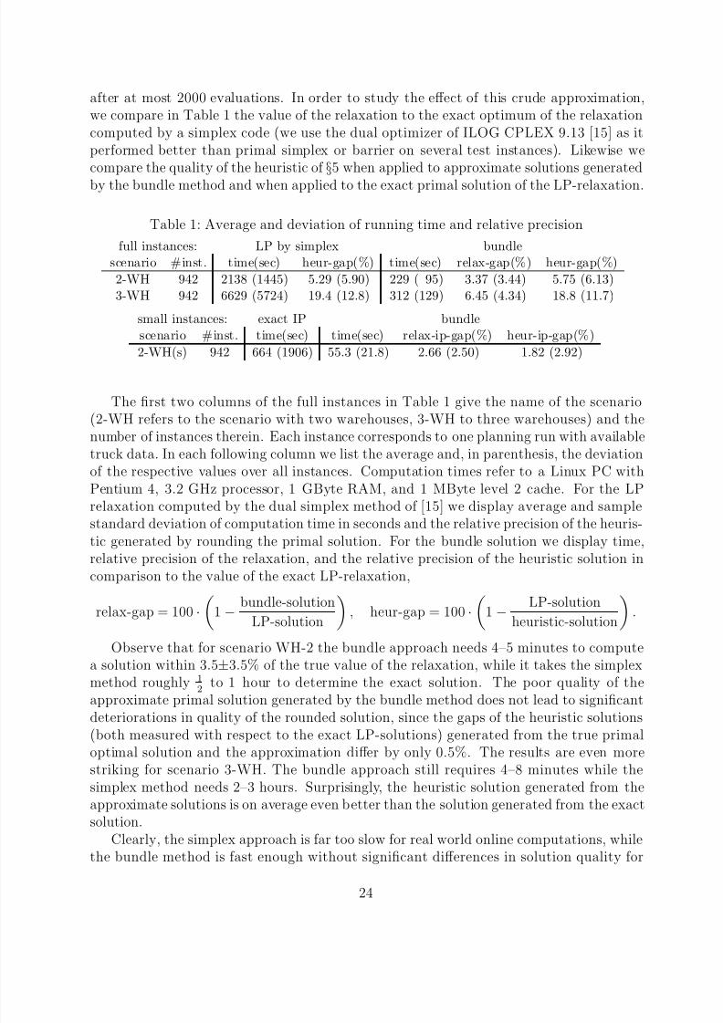
after at most 2000 evaluations. In order to study the effect of this crude approximation,we compare in Table 1 the value of the relaxation to the exact optimum of the relaxationcomputed by a simplex code (we use the dual optimizer of ILOG CPLEX 9.13 [15] as itperformed better than primal simplex or barrier on several test instances). Likewise wecompare the quality of the heuristic of §5 when applied to approximate solutions generatedby the bundle method and when applied to the exact primal solution of the LP-relaxation.
Table 1: Average and deviation of running time and relative precision
full instances: LP by simplex bundlescenario #inst. time(sec) heur-gap(%) time(sec) relax-gap(%) heur-gap(%)
2-WH 942 2138 (1445) 5.29 (5.90) 229 ( 95) 3.37 (3.44) 5.75 (6.13)3-WH 942 6629 (5724) 19.4 (12.8) 312 (129) 6.45 (4.34) 18.8 (11.7)
small instances: exact IP bundlescenario #inst. time(sec) time(sec) relax-ip-gap(%) heur-ip-gap(%)
2-WH(s) 942 664 (1906) 55.3 (21.8) 2.66 (2.50) 1.82 (2.92)
The first two columns of the full instances in Table 1 give the name of the scenario(2-WH refers to the scenario with two warehouses, 3-WH to three warehouses) and thenumber of instances therein. Each instance corresponds to one planning run with availabletruck data. In each following column we list the average and, in parenthesis, the deviationof the respective values over all instances. Computation times refer to a Linux PC withPentium 4, 3.2 GHz processor, 1 GByte RAM, and 1 MByte level 2 cache. For the LPrelaxation computed by the dual simplex method of [15] we display average and samplestandard deviation of computation time in seconds and the relative precision of the heuris-
tic generated by rounding the primal solution. For the bundle solution we display time,relative precision of the relaxation, and the relative precision of the heuristic solution incomparison to the value of the exact LP-relaxation,
relax-gap = 100 ·
1 −
bundle-solution
LP-solution
, heur-gap = 100 ·
1 −
LP-solution
heuristic-solution
.
Observe that for scenario WH-2 the bundle approach needs 4–5 minutes to computea solution within 3.5±3.5% of the true value of the relaxation, while it takes the simplexmethod roughly 1
2to 1 hour to determine the exact solution. The poor quality of the
approximate primal solution generated by the bundle method does not lead to significant
deteriorations in quality of the rounded solution, since the gaps of the heuristic solutions(both measured with respect to the exact LP-solutions) generated from the true primaloptimal solution and the approximation differ by only 0.5%. The results are even morestriking for scenario 3-WH. The bundle approach still requires 4–8 minutes while thesimplex method needs 2–3 hours. Surprisingly, the heuristic solution generated from theapproximate solutions is on average even better than the solution generated from the exactsolution.
Clearly, the simplex approach is far too slow for real world online computations, whilethe bundle method is fast enough without significant differences in solution quality for
24
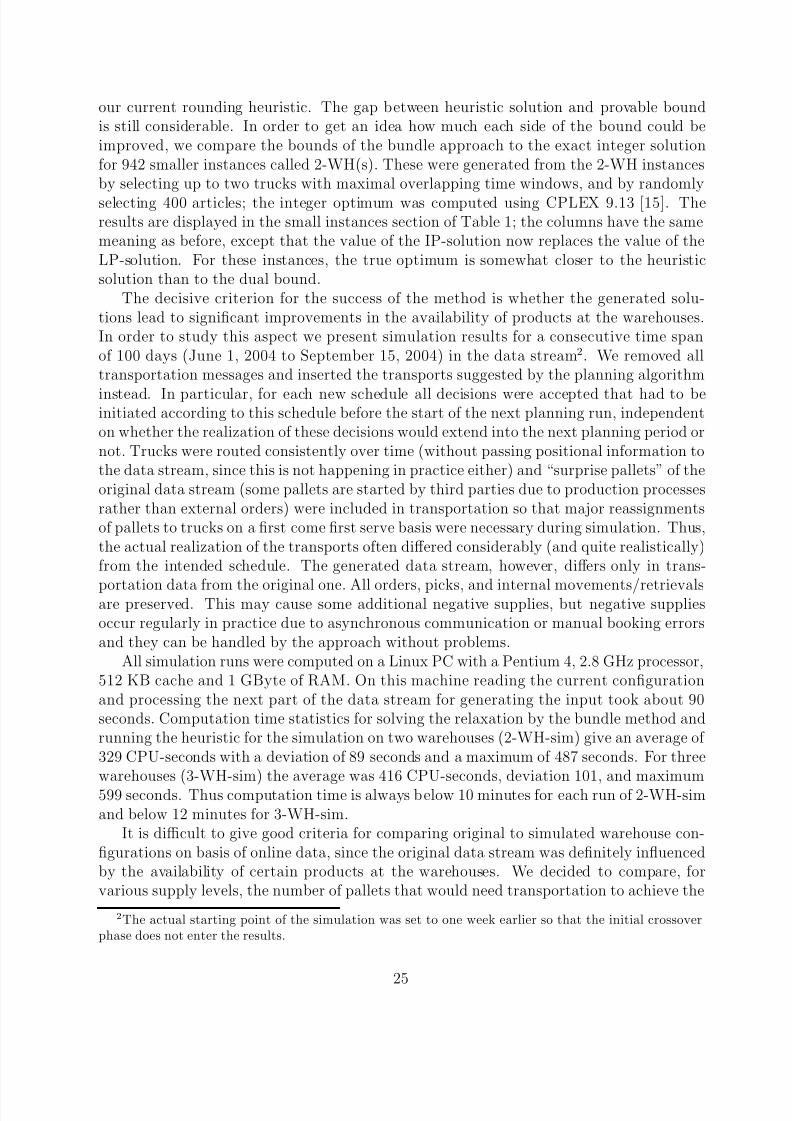
8/3/2019 Pallets and Warehouses Optimization
http://slidepdf.com/reader/full/pallets-and-warehouses-optimization 25/32
our current rounding heuristic. The gap between heuristic solution and provable boundis still considerable. In order to get an idea how much each side of the bound could beimproved, we compare the bounds of the bundle approach to the exact integer solutionfor 942 smaller instances called 2-WH(s). These were generated from the 2-WH instancesby selecting up to two trucks with maximal overlapping time windows, and by randomlyselecting 400 articles; the integer optimum was computed using CPLEX 9.13 [15]. Theresults are displayed in the small instances section of Table 1; the columns have the samemeaning as before, except that the value of the IP-solution now replaces the value of theLP-solution. For these instances, the true optimum is somewhat closer to the heuristicsolution than to the dual bound.
The decisive criterion for the success of the method is whether the generated solu-tions lead to significant improvements in the availability of products at the warehouses.In order to study this aspect we present simulation results for a consecutive time spanof 100 days (June 1, 2004 to September 15, 2004) in the data stream 2. We removed alltransportation messages and inserted the transports suggested by the planning algorithm
instead. In particular, for each new schedule all decisions were accepted that had to beinitiated according to this schedule before the start of the next planning run, independenton whether the realization of these decisions would extend into the next planning period ornot. Trucks were routed consistently over time (without passing positional information tothe data stream, since this is not happening in practice either) and “surprise pallets” of theoriginal data stream (some pallets are started by third parties due to production processesrather than external orders) were included in transportation so that major reassignmentsof pallets to trucks on a first come first serve basis were necessary during simulation. Thus,the actual realization of the transports often differed considerably (and quite realistically)from the intended schedule. The generated data stream, however, differs only in trans-
portation data from the original one. All orders, picks, and internal movements/retrievalsare preserved. This may cause some additional negative supplies, but negative suppliesoccur regularly in practice due to asynchronous communication or manual booking errorsand they can be handled by the approach without problems.
All simulation runs were computed on a Linux PC with a Pentium 4, 2.8 GHz processor,512 KB cache and 1 GByte of RAM. On this machine reading the current configurationand processing the next part of the data stream for generating the input took about 90seconds. Computation time statistics for solving the relaxation by the bundle method andrunning the heuristic for the simulation on two warehouses (2-WH-sim) give an average of 329 CPU-seconds with a deviation of 89 seconds and a maximum of 487 seconds. For threewarehouses (3-WH-sim) the average was 416 CPU-seconds, deviation 101, and maximum599 seconds. Thus computation time is always below 10 minutes for each run of 2-WH-simand below 12 minutes for 3-WH-sim.
It is difficult to give good criteria for comparing original to simulated warehouse con-figurations on basis of online data, since the original data stream was definitely influencedby the availability of certain products at the warehouses. We decided to compare, forvarious supply levels, the number of pallets that would need transportation to achieve the
2The actual starting point of the simulation was set to one week earlier so that the initial crossoverphase does not enter the results.
25
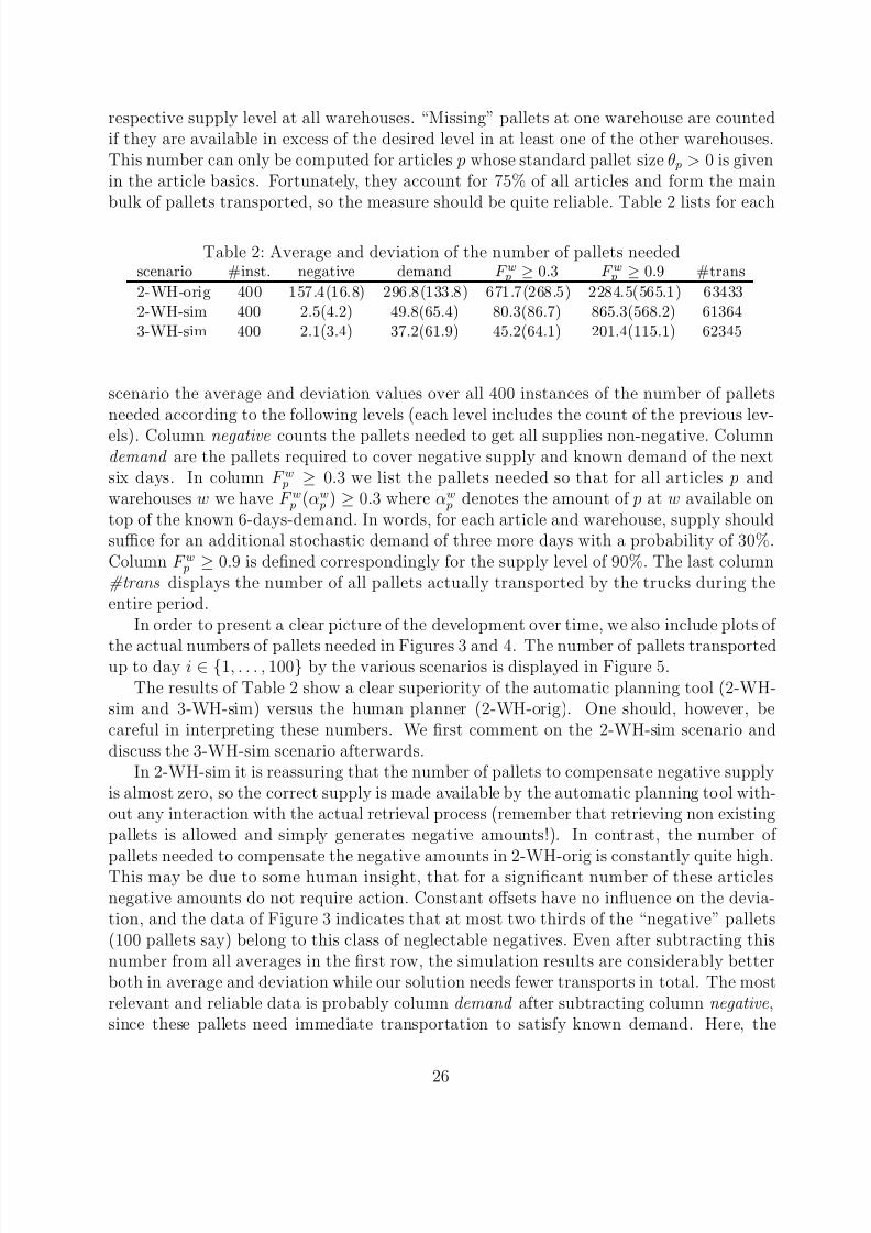
8/3/2019 Pallets and Warehouses Optimization
http://slidepdf.com/reader/full/pallets-and-warehouses-optimization 26/32
respective supply level at all warehouses. “Missing” pallets at one warehouse are countedif they are available in excess of the desired level in at least one of the other warehouses.This number can only be computed for articles p whose standard pallet size θ p > 0 is givenin the article basics. Fortunately, they account for 75% of all articles and form the mainbulk of pallets transported, so the measure should be quite reliable. Table 2 lists for each
Table 2: Average and deviation of the number of pallets neededscenario #inst. negative demand F w p ≥ 0.3 F w p ≥ 0.9 #trans
2-WH-orig 400 157.4(16.8) 296.8(133.8) 671.7(268.5) 2284.5(565.1) 634332-WH-sim 400 2.5(4.2) 49.8(65.4) 80.3(86.7) 865.3(568.2) 613643-WH-sim 400 2.1(3.4) 37.2(61.9) 45.2(64.1) 201.4(115.1) 62345
scenario the average and deviation values over all 400 instances of the number of palletsneeded according to the following levels (each level includes the count of the previous lev-
els). Column negative counts the pallets needed to get all supplies non-negative. Columndemand are the pallets required to cover negative supply and known demand of the nextsix days. In column F w p ≥ 0.3 we list the pallets needed so that for all articles p andwarehouses w we have F w p (αw
p ) ≥ 0.3 where αw p denotes the amount of p at w available on
top of the known 6-days-demand. In words, for each article and warehouse, supply shouldsuffice for an additional stochastic demand of three more days with a probability of 30%.Column F w p ≥ 0.9 is defined correspondingly for the supply level of 90%. The last column#trans displays the number of all pallets actually transported by the trucks during theentire period.
In order to present a clear picture of the development over time, we also include plots of
the actual numbers of pallets needed in Figures 3 and 4. The number of pallets transportedup to day i ∈ {1, . . . , 100} by the various scenarios is displayed in Figure 5.
The results of Table 2 show a clear superiority of the automatic planning tool (2-WH-sim and 3-WH-sim) versus the human planner (2-WH-orig). One should, however, becareful in interpreting these numbers. We first comment on the 2-WH-sim scenario anddiscuss the 3-WH-sim scenario afterwards.
In 2-WH-sim it is reassuring that the number of pallets to compensate negative supplyis almost zero, so the correct supply is made available by the automatic planning tool with-out any interaction with the actual retrieval process (remember that retrieving non existingpallets is allowed and simply generates negative amounts!). In contrast, the number of
pallets needed to compensate the negative amounts in 2-WH-orig is constantly quite high.This may be due to some human insight, that for a significant number of these articlesnegative amounts do not require action. Constant offsets have no influence on the devia-tion, and the data of Figure 3 indicates that at most two thirds of the “negative” pallets(100 pallets say) belong to this class of neglectable negatives. Even after subtracting thisnumber from all averages in the first row, the simulation results are considerably betterboth in average and deviation while our solution needs fewer transports in total. The mostrelevant and reliable data is probably column demand after subtracting column negative,since these pallets need immediate transportation to satisfy known demand. Here, the
26
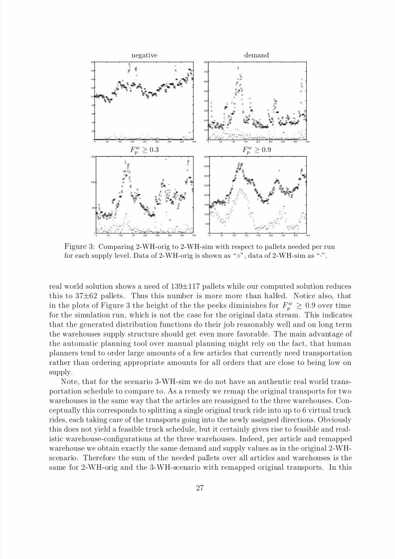
8/3/2019 Pallets and Warehouses Optimization
http://slidepdf.com/reader/full/pallets-and-warehouses-optimization 27/32
negative demand
0 50 100 150 200 250 300 350 4000
20
40
60
80
100
120
140
160
180
0 50 100 150 200 250 300 350 4000
100
200
300
400
500
600
700
800
F w p ≥ 0.3 F w p ≥ 0.9
0 50 100 150 200 250 300 350 4000
500
1000
1500
0 50 100 150 200 250 300 350 4000
500
1000
1500
2000
2500
3000
3500
4000
Figure 3: Comparing 2-WH-orig to 2-WH-sim with respect to pallets needed per runfor each supply level. Data of 2-WH-orig is shown as “◦”, data of 2-WH-sim as “·”.
real world solution shows a need of 139±117 pallets while our computed solution reduces
this to 37±62 pallets. Thus this number is more more than halfed. Notice also, thatin the plots of Figure 3 the height of the the peeks diminishes for F w p ≥ 0.9 over timefor the simulation run, which is not the case for the original data stream. This indicatesthat the generated distribution functions do their job reasonably well and on long termthe warehouses supply structure should get even more favorable. The main advantage of the automatic planning tool over manual planning might rely on the fact, that humanplanners tend to order large amounts of a few articles that currently need transportationrather than ordering appropriate amounts for all orders that are close to being low onsupply.
Note, that for the scenario 3-WH-sim we do not have an authentic real world trans-
portation schedule to compare to. As a remedy we remap the original transports for twowarehouses in the same way that the articles are reassigned to the three warehouses. Con-ceptually this corresponds to splitting a single original truck ride into up to 6 virtual truckrides, each taking care of the transports going into the newly assigned directions. Obviouslythis does not yield a feasible truck schedule, but it certainly gives rise to feasible and real-istic warehouse-configurations at the three warehouses. Indeed, per article and remappedwarehouse we obtain exactly the same demand and supply values as in the original 2-WH-scenario. Therefore the sum of the needed pallets over all articles and warehouses is thesame for 2-WH-orig and the 3-WH-scenario with remapped original transports. In this
27
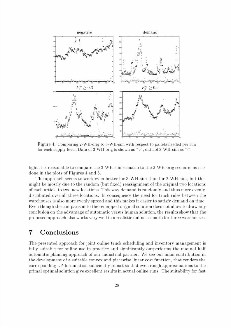
8/3/2019 Pallets and Warehouses Optimization
http://slidepdf.com/reader/full/pallets-and-warehouses-optimization 28/32
negative demand
0 50 100 150 200 250 300 350 4000
20
40
60
80
100
120
140
160
180
0 50 100 150 200 250 300 350 4000
100
200
300
400
500
600
700
800
F w p ≥ 0.3 F w p ≥ 0.9
0 50 100 150 200 250 300 350 4000
500
1000
1500
0 50 100 150 200 250 300 350 4000
500
1000
1500
2000
2500
3000
3500
4000
Figure 4: Comparing 2-WH-orig to 3-WH-sim with respect to pallets needed per runfor each supply level. Data of 2-WH-orig is shown as “◦”, data of 3-WH-sim as “·”.
light it is reasonable to compare the 3-WH-sim scenario to the 2-WH-orig scenario as it is
done in the plots of Figures 4 and 5.The approach seems to work even better for 3-WH-sim than for 2-WH-sim, but this
might be mostly due to the random (but fixed) reassignment of the original two locationsof each article to two new locations. This way demand is randomly and thus more evenlydistributed over all three locations. In consequence the need for truck rides between thewarehouses is also more evenly spread and this makes it easier to satisfy demand on time.Even though the comparison to the remapped original solution does not allow to draw anyconclusion on the advantage of automatic versus human solution, the results show that theproposed approach also works very well in a realistic online scenario for three warehouses.
7 Conclusions
The presented approach for joint online truck scheduling and inventory management isfully suitable for online use in practice and significantly outperforms the manual half automatic planning approach of our industrial partner. We see our main contribution inthe development of a suitable convex and piecewise linear cost function, that renders thecorresponding LP-formulation sufficiently robust so that even rough approximations to theprimal optimal solution give excellent results in actual online runs. The suitability for fast
28
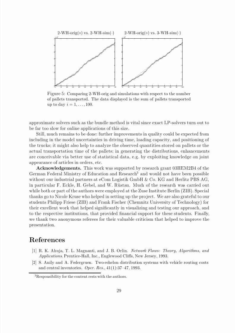
8/3/2019 Pallets and Warehouses Optimization
http://slidepdf.com/reader/full/pallets-and-warehouses-optimization 29/32
2-WH-orig(◦) vs. 2-WH-sim(·) 2-WH-orig(◦) vs. 3-WH-sim(·)
0 10 20 30 40 50 60 70 80 90 1000
1
2
3
4
5
6
7x 10
4
0 10 20 30 40 50 60 70 80 90 1000
1
2
3
4
5
6
7x 10
4
Figure 5: Comparing 2-WH-orig and simulations with respect to the numberof pallets transported. The data displayed is the sum of pallets transportedup to day i = 1, . . . , 100.
approximate solvers such as the bundle method is vital since exact LP-solvers turn out tobe far too slow for online applications of this size.
Still, much remains to be done: further improvements in quality could be expected fromincluding in the model uncertainties in driving time, loading capacity, and positioning of the trucks; it might also help to analyze the observed quantities stored on pallets or theactual transportation time of the pallets; in generating the distributions, enhancementsare conceivable via better use of statistical data, e.g. by exploiting knowledge on jointappearance of articles in orders, etc.
Acknowledgements. This work was supported by research grant 03HEM2B4 of the
German Federal Ministry of Education and Research3
and would not have been possiblewithout our industrial partners at eCom Logistik GmbH & Co. KG and Herlitz PBS AG,in particular F. Eckle, H. Gebel, and W. Rustau. Much of the research was carried outwhile both or part of the authors were employed at the Zuse Institute Berlin (ZIB). Specialthanks go to Nicole Kruse who helped in setting up the project. We are also grateful to ourstudents Philipp Friese (ZIB) and Frank Fischer (Chemnitz University of Technology) fortheir excellent work that helped significantly in visualizing and testing our approach, andto the respective institutions, that provided financial support for these students. Finally,we thank two anonymous referees for their valuable criticism that helped to improve thepresentation.
References
[1] R. K. Ahuja, T. L. Magnanti, and J. B. Orlin. Network Flows: Theory, Algorithms, and
Applications. Prentice-Hall, Inc., Englewood Cliffs, New Jersey, 1993.
[2] S. Anily and A. Federgruen. Two-echelon distribution systems with vehicle routing costsand central inventories. Oper. Res., 41(1):37–47, 1993.
3Responsibility for the content rests with the authors.
29
8/3/2019 Pallets and Warehouses Optimization
http://slidepdf.com/reader/full/pallets-and-warehouses-optimization 30/32
[3] T. W. Archibald, S. A. E. Sassen, and L. C. Thomas. An optimal policy for a two depotinventory problem with stock transfer. Manage. Sci., 43(2):173–183, 1997.
[4] A. Ben-Tal and A. Nemirovski. Robust optimization – methodology and applications.Math. Programming , 92(3):453–480, 2002.
[5] J. Boudoukh, M. Richardson, and R. Whitelaw. The Best of Both Worlds: A Hybrid Ap-
proach to Calculating Value at Risk . Risk, 1998. Reprint in Internal Modeling and CADII:Qualifying and Quantifying Risk within a Financial Institution (Risk Books, London, Eng-land), 1999.
[6] S. Feltenmark and K. C. Kiwiel. Dual applications of proximal bundle methods, includingLagrangian relaxation of nonconvex problems. SIAM J. Optim., 10(3):697–721, 2000.
[7] E. H. Frazelle, S. T. Hackman, U. Passy, and L. K. Platzman. The forward-reserve problem.In Proceedings of the 1992 IBM Europe Institute on optimization solutions, pages 43–61,Oberlech, Austria, 1994.
[8] F. Fumero and C. Vercellis. Synchronized development of production, inventory, and dis-tribution schedules. Transp. Sci., 33(3):330–340, 1999.
[9] S. Graves, A. Rinnooy Kan, and P. Zipkin, editors. Logistics of production and inventory ,volume 4 of Handbooks in Operations Research and Management Science. North-Holland,Amsterdam, 1993.
[10] P. Hall. The Bootstrap and Edgeworth Expansions. Springer, New York, 1992.
[11] C. Helmberg. ConicBundle 0.1. Fakultat fur Mathematik, Technische Universitat Chemnitz,2005. http://www.tu-chemnitz.de/∼helmberg/ConicBundle
[12] C. Helmberg and K. C. Kiwiel. A spectral bundle method with bounds. Math. Programming ,93(2):173–194, 2002.
[13] C. Helmberg and S. Rohl. A case study of joint online truck scheduling and inventorymanagement for multiple warehouses. Preprint 2005-3, Technische Universitat Chemnitz,
Fakultat fur Mathematik, Jan. 2005.[14] J.-B. Hiriart-Urruty and C. Lemarechal. Convex Analysis and Minimization Algorithms II ,
volume 306 of Grundlehren der mathematischen Wissenschaften . Springer, Berlin, Heidel-berg, 1993.
[15] ILOG S.A., 9 Rue de Verdun, 94253 Gentilly Cedex, France. ILOG AMPL CPLEX System,
Version 9.1, User’s Guide, Apr. 2005. Information available at http://www.ilog.com.
[16] P. Kochel. Ein dynamisches Mehr-Lager-Modell mit Transportbeziehungen zwischen denLagern. Math. Operationsforsch. Statist., Ser. Optimization , 13:267–286, 1982.
[17] P. Kochel. Optimal adaptive inventory control for a multi-location model with redistribution.Optimization , 19:525–537, 1988.
[18] B. Korte and J. Vygen. Combinatorial optimization. Theory and algorithms, volume 21 of Algorithms and Combinatorics. Springer, Berlin, 2 edition, 2002.
[19] A. Lobel. MCF Version 1.2 – A network simplex Implementation . Zuse Institute Berlin,Jan. 2000. Available at http://www.zib.de/Optimization/Software/Mcf (free of chargefor academic use).
[20] M. Padberg. Linear optimization and extensions, volume 12 of Algorithms and Combina-
torics. Springer, 2nd edition, 1999.
[21] M. I. Reiman, R. Rubio, and L. M. Wein. Heavy traffic analysis of the dynamic stochasticinventory-routing problem. Transp. Sci., 33(4):361–380, 1999.
30
8/3/2019 Pallets and Warehouses Optimization
http://slidepdf.com/reader/full/pallets-and-warehouses-optimization 31/32
[22] W. Romisch and R. Schultz. Multistage stochastic integer programs: An introduction. InM. Groetschel, S. Krumke, and J. Rambau, editors, Online Optimization of Large Scale
Systems, pages 579–598. Springer-Verlag, Berlin, 2001.
[23] A. Schrijver. Combinatorial Optimization , volume 24 of Algorithms and Combinatorics.Springer, 2003.
[24] R. Schultz. Stochastic programming with integer variables. Math. Programming , 97(1-2):285–309, 2003.
[25] J. Shao. Mathematical Statistics. Springer Texts in Statistics. Springer-Verlag, New York,Berlin, Heidelberg, 2nd edition, 2003.
[26] B. W. Silverman. Density estimation for statistics and data analysis. Monographs onStatistics and Applied Probability. Chapman and Hall, New York, 1986.
[27] J. P. van den Berg, G. P. Sharp, A. J. R. M. (Noud) Gademann, and Y. Pochet. Forward-reserve allocation in a warehouse with unit-load replenishments. Europ. J. Oper. Res.,111:98–113, 1998.
[28] M. H. van der Vlerk. Convex approximations for complete integer recourse models.Math. Programming , 99(2):297–310, 2004.
31
8/3/2019 Pallets and Warehouses Optimization
http://slidepdf.com/reader/full/pallets-and-warehouses-optimization 32/32
A Notation
N,Z,R natural, integer, real numbersT = {ti : 1 ≤ i ≤ nT } time discretization, 0 ≤ t1 < .. . < tnT
R set of truck classes (w.r.t. loading properties and availability)
W , W d set of warehouses, set of warehouses including truck depot dP set of products/articles W ⊂ W × W set of directions needed for prescheduled pallets
V h, h ∈ R ∪ P ∪ W sets of nodes, subset of triples from W d × {A,B,C,L,U } × T v = (vW , vN , vT ) ∈ V h node components are indexed by W arehouse, N ame, T ime
Ah, h ∈ R ∪ P ∪ W multiset of arcs, subset of V h × V ha = (u, v) an arcDr(V r, Ar), r ∈ R truck graphsD p(V p, A p), p ∈ P article graphs
D w(V w, A w), w ∈ W prescheduled pallets graphs
bh ∈ ZV h balances of network Dh
lh, uh ∈ ZAh lower and upper bounds on the arcs in network Dh T ⊂ T selected time steps for convex cost terms
Af = P × W × T index set of variables for these cost termsx( p,w,t) number of pallets of p available at w if transports stop at t
A = Af ∪
j∈R∪P∪ W
A j index set of all variables (disjoint union)
c ∈ RA\Af cost vector of the arcs in the networks
θ p typical or standard amount on a pallet of article p ∈ P αw p remainder amount after rounding supply and demand
of p ∈ P at w ∈ W to standard pallets, typically αw p ∈ [0, θ p)γ = 1000 large value for penalizing infeasibilities in the cost functionε = 0.01 small value for minor preferences in the cost functionπ = 0.9 if expected demand is covered with this probability,
no further pallets should be brought in.π = 0.01 if expected demand is covered with at most this probability,
priority 3 pallets are rated with a constant large priorityF w p (α) distribution function giving probability that
amount α satisfies future demand for article p at warehouse wπw p ( j) = 1 − F w p (αw
p + jθ p), Prob(all up to the j-th pallet are needed)
f w p (x( p,w,t)) expected number of pallets of p needed at w if transportstops after t
f w p (x( p,w,t)) cost function derived from transformed f w p (x( p,w,t))dwi,p demand for p at w on the i-th previous workday
Gw,m p distribution function of the sum of demand for p at w over
the next m workdays
Gw,m p estimation of Gw,m
p by empirical distribution functionϕ(y), ϕi(y) dual function of the LP-relaxation or of block i in it
32