paged overlay 1 7 - IARIA Journals · Michael A. Bauer, TheUniversity ofWestern Ontario , Canada 54...

The International Journal On Advances in Intelligent Systems is Published by IARIA.

ISSN: 1942-2679

journals site: http://www.iariajournals.org

contact: [email protected]

Responsibility for the contents rests upon the authors and not upon IARIA, nor on IARIA volunteers,

staff, or contractors.

IARIA is the owner of the publication and of editorial aspects. IARIA reserves the right to update the

content for quality improvements.

Abstracting is permitted with credit to the source. Libraries are permitted to photocopy or print,

providing the reference is mentioned and that the resulting material is made available at no cost.

Reference should mention:

International Journal On Advances in Intelligent Systems, issn 1942-2679

vol. 1, no. 1, year 2008, http://www.iariajournals.org/intelligent_systems/"

The copyright for each included paper belongs to the authors. Republishing of same material, by authors

or persons or organizations, is not allowed. Reprint rights can be granted by IARIA or by the authors, and

must include proper reference.

Reference to an article in the journal is as follows:

<Author list>, “<Article title>”

International Journal On Advances in Intelligent Systems, issn 1942-2679

vol. 1, no. 1, year 2008,<start page>:<end page> , http://www.iariajournals.org/intelligent_systems/"

IARIA journals are made available for free, proving the appropriate references are made when their

content is used.

Sponsored by IARIA

www.iaria.org

Copyright © 2008 IARIA

International Journal On Advances in Intelligent Systems

Volume 1, Number 1, 2008

Editorial Board

First Issue Coordinators

Jaime Lloret, Universidad Politécnica de Valencia, Spain

Pascal Lorenz, Université de Haute Alsace, France

Petre Dini, Cisco Systems, Inc., USA / Concordia University, Canada

Autonomus and Autonomic Systems

Michael Bauer, The University of Western Ontario, Canada

Radu Calinescu, Oxford University, UK

Larbi Esmahi, Athabasca University, Canada

Florin Gheorghe Filip, Romanian Academy, Romania

Adam M. Gadomski, ENEA, Italy

Alex Galis, University College London, UK

Michael Grottke, University of Erlangen-Nuremberg, Germany

Nhien-An Le-Khac, University College Dublin, Ireland

Fidel Liberal Malaina, University of the Basque Country, Spain

Jeff Riley, Hewlett-Packard Australia, Australia

Rainer Unland, University of Duisburg-Essen, Germany

Advanced Computer Human Interactions

Freimut Bodendorf, University of Erlangen-Nuernberg Germany

Daniel L. Farkas, Cedars-Sinai Medical Center - Los Angeles, USA

Janusz Kacprzyk, Polish Academy of Sciences, Poland

Lorenzo Masia, Italian Institute of Technology (IIT) - Genova, Italy

Antony Satyadas, IBM, USA

Advanced Information Processing Technologies

Mirela Danubianu, "Stefan cel Mare" University of Suceava, Romania

Kemal A. Delic, HP Co., USA

Sorin Georgescu, Ericsson Research, Canada

Josef Noll, UiO/UNIK, Sweden

Liviu Panait, Google Inc., USA

Kenji Saito, Keio University, Japan

Thomas C. Schmidt, University of Applied Sciences – Hamburg, Germany

Karolj Skala, Rudjer Bokovic Institute - Zagreb, Croatia

Chieh-yih Wan, Intel Corporation, USA

Hoo Chong Wei, Motorola Inc, Malaysia

Ubiquitous Systems and Technologies

Matthias Bohmer, Munster University of Applied Sciences, Germany

Dominic Greenwood, Whitestein Technologies AG, Switzerland

Arthur Herzog, Technische Universitat Darmstadt, Germany

Reinhard Klemm, Avaya Labs Research-Basking Ridge, USA

Said Tazi, LAAS-CNRS, Universite Toulouse 1, France

Advanced Computing

Dumitru Dan Burdescu, University of Craiova, Romania

Simon G. Fabri, University of Malta – Msida, Malta

Matthieu Geist, Supelec / ArcelorMittal, France

Jameleddine Hassine, Cisco Systems, Inc., Canada

Sascha Opletal, Universitat Stuttgart, Germany

Flavio Oquendo, European University of Brittany - UBS/VALORIA, France

Meikel Poess, Oracle, USA

Said Tazi, LAAS-CNRS, Universite de Toulouse / Universite Toulouse1, France

Antonios Tsourdos, Cranfield University/Defence Academy of the United Kingdom, UK

Centric Systems and Technologies

Razvan Andonie, Central Washington University - Ellensburg, USA / Transylvania University of

Brasov, Romania

Kong Cheng, Telcordia Research, USA

Vitaly Klyuev, University of Aizu, Japan

Josef Noll, ConnectedLife@UNIK / UiO- Kjeller, Norway

Willy Picard, The Poznan University of Economics, Poland

Roman Y. Shtykh, Waseda University, Japan

Weilian Su, Naval Postgraduate School - Monterey, USA

GeoInformation and Web Services

Christophe Claramunt, Naval Academy Research Institute, France

Wu Chou, Avaya Labs Fellow, AVAYA, USA

Suzana Dragicevic, Simon Fraser University, Canada

Dumitru Roman, Semantic Technology Institute Innsbruck, Austria

Emmanuel Stefanakis, Harokopio University, Greece

Semantic Processing

Marsal Gavalda, Nexidia Inc.-Atlanta, USA & CUIMPB-Barcelona, Spain

Christian F. Hempelmann, RiverGlass Inc. - Champaign & Purdue University - West Lafayette,

USA

Josef Noll, ConnectedLife@UNIK / UiO- Kjeller, Norway

Massimo Paolucci, DOCOMO Communications Laboratories Europe GmbH – Munich, Germany

Tassilo Pellegrini, Semantic Web Company, Austria

Antonio Maria Rinaldi, Universita di Napoli Federico II - Napoli Italy

Dumitru Roman, University of Innsbruck, Austria

Umberto Straccia, ISTI – CNR, Italy

Rene Witte, Concordia University, Canada

Peter Yeh, Accenture Technology Labs, USA

Filip Zavoral, Charles University in Prague, Czech Republic



Foreword

Finally, we did it! It was a long exercise to have this inaugural number of the journal featuring extended

versions of selected papers from the IARIA conferences.

With this 2008, Vol. 1 No.1, we open a long series of hopefully interesting and useful articles on

advanced topics covering both industrial tendencies and academic trends. The publication is by-

invitation-only and implies a second round of reviews, following the first round of reviews during the

paper selection for the conferences.

Starting with 2009, quarterly issues are scheduled, so the outstanding papers presented in IARIA

conferences can be enhanced and presented to a large scientific community. Their content is freely

distributed from the www.iariajournals.org and will be indefinitely hosted and accessible to everybody

from anywhere, with no password, membership, or other restrictive access.

We are grateful to the members of the Editorial Board that will take full responsibility starting with the

2009, Vol 2, No1. We thank all volunteers that contributed to review and validate the contributions for

the very first issue, while the Board was getting born. Starting with 2009 issues, the Editor-in Chief will

take this editorial role and handle through the Editorial Board the process of publishing the best

selected papers.

Some issues may cover specific areas across many IARIA conferences or dedicated to a particular

conference. The target is to offer a chance that an extended version of outstanding papers to be

published in the journal. Additional efforts are assumed from the authors, as invitation doesn’t

necessarily imply immediate acceptance.

This particular issue covers papers invited from those presented in 2007 and early 2008 conferences.

The papers reflect the evolution of the society from advanced use of the technology for education to

user-centric aspects in socio-semantic networks, and complexity of the new environments dealing with

adaptive monitoring, load-balancing, and policy-driven autonomic computing.

We hope in a successful launching and expect your contributions via our events.

First Issue Coordinators,

Jaime Lloret, Universidad Politécnica de Valencia, Spain

Pascal Lorenz, Université de Haute Alsace, France

Petre Dini, Cisco Systems, Inc., USA / Concordia University, Canada



CONTENTS

Development and Educational Practice of a Lunar Observation Support System by using

Mobile Phones for Science Education

Hitoshi Miyata, Shiga University, Japan

Mariko Suzuki, Shiga University, Japan

Michiko Fukahori, Settsu 1st Junior High School, Japan

Tatusuhiko Akamatsu, ASK Asset Consulting Inc., Japan

1 - 10

Polling Schedule Optimization for Adaptive Monitoring to Scalable Enterprise Systems

Fumio Machida, NEC Service Platforms Research Laboratories, Japan

Masahiro Kawato, NEC Service Platforms Research Laboratories, Japan

Yoshiharu Maeno, NEC Service Platforms Research Laboratories, Japan

11 - 22

Effective Design of Trust Ontologies for Improvement in the Structure of Socio-Semantic

Trust Networks

Nima Dokoohaki, Royal Institute of Technology (KTH), Sweden

Mihhail Matskin, Royal Institute of Technology (KTH), Sweden // Norwegian University of Science

and Technology, (NTNU), Norway

23 - 42

On Choosing a Load-Balancing Algorithm for Parallel Systems with Temporal Constraints

Luís Fernando Orleans, Federal University of Rio of Janeiro, Brazil

Geraldo Zimbrão, Federal University of Rio of Janeiro, Brazil

Pedro Furtado, University of Coimbra, Portugal

43 - 53

Modelling Reinforcement Learning in Policy-driven Autonomic Management

Raphael M. Bahati, The University of Western Ontario , Canada

Michael A. Bauer, The University of Western Ontario , Canada

54 - 79

1

International Journal On Advances in Intelligent Systems, vol 1 no 1, year 2008, http://www.iariajournals.org/intelligent_systems/

Development and Educational Practice of a Lunar Observation Support System by using Mobile Phones for Science Education

Hitoshi MIYATA, Mariko Suzuki Michiko Fukahori Tatusuhiko Akamatsu

Shiga University Settsu 1st Junior High School ASK Asset Consulting Inc. 2-5-1, Hiratsu, Otsu, Shiga 3-20,Minamisenrioka, Settsu, Osaka 2-1-10, Andoji-machi, Osaka

JAPAN JAPAN JAPAN [email protected] [email protected] [email protected] [email protected]

Abstract

A Lunar Observation Project that utilizes mobile phones was undertaken with junior high school students as the subjects. A “Lunar Observation Support System” that can be used with mobile phones was developed. Using this system, students observe the Moon in the open air and send observational data through their mobile phones to the server; the server automatically stores the data in a database. The system also possesses a Computer-Supported Collaborative Learning (CSCL) feature through which students can share observational data with each other and engage in discussions. From a practical study, we found that students were able to send lunar observational data from their mobile phones effortlessly from the outdoors, and their interest, attention, attitude, and motivation toward nature observation improved. In addition, sharing each student’s observational record on the Web Database and engaging the students in discussions led to the correction of simple false beliefs that students often have, such as “the Moon can be seen only during the night” and “the Moon rises at the same time everyday.” Key Words: u-Learning, Mobile Phone, CSCL, Web Database, Observational Studies, Science Education 1. Introduction

In Japanese education, growth of science communication among various people is an urgent need. Ministry of Education, Culture, Sports, Science and Technology has struggled to enhance science communication among various people, involving elementary, junior high and senior high school students, college students, graduate students and experts (Ministry of Education, Culture, Sports, Science and Technology, 2006) [1]. The Science Council of Japan, moreover, has stated that it is necessary to foster science communicators, including prospective teachers and science volunteers (The Science Council of Japan, 2007) [2]. To contribute toward mitigating this social issue in Japan, authors have focused on the moon as a popular scientific topic in astronomy.

It is not easy for both children and adults to

communicate about astronomical phenomena. Many investigators have examined students' ideas of the relationships among the moon, earth, and sun (for example, Vosniadou and Brewer, 1994; Agata, 2004) [3] [4]. Prospective elementary school teachers frequently hold similar problematic conceptions of cosmic relationships (for example, Atwood & Atwood, 1997; Suzuki, 2003) [5] [6].

On-going observation and conversation have the possibility of enhancing college students to understand the phases of the moon (Suzuki, 2003). In another research (Suzuki, et al., 2006), most of students seemed to value the experience of making observations, sharing observational data and developing explanations of the moon. Some, however, showed resistance to recording and observing the moon outside the classes, and that they couldn’t do this, even though they realized that observations of the moon would be useful for learning about the moon [7]. Reasons could be awkward to write down observational records on paper in the field and; there are differences among individuals’ writings of the same moon.

Authors developed the LOS system consists of a mobile part and a sharing part on PCs to facilitate students’ ability to continue observation of the moon, to share observations and to converse about them. Using the LOS system, users observe the moon in the open air and send observational data through their mobile devices to the server; the server automatically stores the data in a database. (Miyata et. al., 2007; Suzuki et. al., 2007) [8] [9].

Personal, portable, wirelessly-networked technologies have created the potential for a new phase in the evolution of technology-enhanced learning, marked by a continuity of the learning experience across different environments. Many education support systems by ubiquitous access to mobile, connected, personal, handhelds have been developed (Chan, et al., 2006) [10]. Ways to use movable devices such as a PDA and a mobile phone for fieldwork and project based learning have been examined. For example, the collect system by O’Hara, et al. (2007) consists of a mobile application, a series of situated signs and a personalized web page [11]. Haapala, et al. (2007) studied parallel collaborative learning

2


between students in the classroom using a PC computer and students in the field using a mobile device [12]. In Japan, Takenaka, et al. (2006) developed the sharing information system on a website by sending pictures taken with mobile phones as e-mail attachments [13]. These studies examined the effects of systems which provide users observing frameworks through mobile devices and/or collect user’s observational data for sharing.

The LOS system possesses two features; 1) a scaffolding feature to enhance users’ deliberating on the phases of the moon and 2) a CSCL (Computer-Supported Collaborative Learning) feature through which users can share observational data on PCs with each other and engage in discussions.

We did two practices for 10 junior & senior high school students (Miyata, et al., 2007) and for 15 college students (Suzuki, et al., 2007). In the study for 10 junior & senior high school students, they observed the moon, interacted mainly with an on-line facilitator and shared the observational data with other participants via internet. The study for 15 college students was implemented in a part of a course for prospective teachers. They observed the moon out of the classroom and also communicated with each other in the classes. In this paper, we discuss about both the junior & senior high school course and university course to evaluate the LOS system, when incorporated into fieldwork and project based learning inside and outside of a classroom. 2. Objective of this Research

We developed a “Lunar Observation Support System” that utilizes the capability of mobile phones to access the Web and in which students can submit observational data of the Moon. We also developed a Web-based educational material entitled “Moon Observation Project” in which the uploaded observational data is automatically stored in a database and can be viewed in real time. The objectives of this research are to validate and analyze the usability of the Lunar Observation Support System as a learning tool and to understand whether by using the tool and employing junior and senior high school students as subjects, there are any effects on the students in nature observation classes; in particular, we study their knowledge, understanding, thinking, judgment, interest, attention, attitude, and motivation with regard to the study of the Moon. 3. Research Method

We analyzed the effectiveness of the Lunar Observation Support System by employing students from grade 1st of junior high school to grade 1st of senior high school as subjects and by using data collected from a nature observation class that utilized the system. In particular, we validated and analyzed the effect of utilizing the mobile phone for recording lunar

observations on the students with respect to changes in the their knowledge, understanding, thinking, judgment, interest, attention, attitude, and motivation. 3.1. Subjects

The subjects comprised students from grade 1st of junior high school to grade 1st of senior high school (8 boys and 2 girls) 3.2. Orientation for lunar observation and the investigation process

We explained the usage of the Moon Observation Support System on December 9, 2006 at Shiga University using handouts. In addition, in order to investigate the students’ knowledge of the Moon before beginning the observations, we administered a test entitled “Survey on the Appearance of the Moon,” which was based on the Lunar Phases Concept Inventory (LPCI). 3.3. Observation period

The observation period was from December 9 to December 30, 2006 (approximately 3 weeks or 22 days). 3.4. Notes on data collection and analysis 3.4.1. Lunar Phases Concept Inventory (LPCI)

LPCI is a survey questionnaire comprising 20 multiple-choice questions concerning the phases of the Moon. The survey was developed by Lindell et al [14]. According to Lindell et al. (2002), the survey is suitable for analyzing the conceptual knowledge that university students have on lunar phases. Since the accuracy rate for LPCI is not high even for university students, we selected 11 questions out of the 20, taking into consideration the fact that junior and senior high school students will be answering these questions. The test based on LPCI and entitled “Survey on the Appearance of the Moon” was administered before the observation period began, and it was administered again after the three-week observation period as a post-observation survey. 3.4.2. Paper-based questionnaire

At the end of the three-week observation period, we asked the students to complete a questionnaire that consisted of 14 three-choice and four-choice questions and a free-text question. The questionnaire was designed to elicit the students’ opinions on the use of a mobile phone for entering observational records and on viewing the records using a PC as well as on the usability of the Web site of the Lunar Observation Support System for mobile phones. 4. Structure and Content of the Lunar Observation Support System 4.1. Lunar Observation Support System for mobile phones ( http://mb.cerp.shiga-u.ac.jp/moon/m/ )

The present system comprises the Web site entitled “Lunar Observation Support System,” the administrative interface for downloading the submitted data, and the database server in which the data is stored.

The Web site consists of the following pages: “Top page (Fig.1),” “Enter observational record, (Fig.2),” “Select the phase, (Fig. 3)” “Adjust the slant and phase,” “Confirm selection and enter observational note,” and the “Submission complete”.

3


In the “Adjust the slant and phase” screen shown in Figure 4, a large graphic of the Moon with the selected phase is displayed, and the user can increment or decrement the slant in 15° intervals up to 90°. The user adjusts the slant of the Moon to the angle closest to his/her observation. Further, the user can finely adjust the phase of the Moon, which was selected in Figure 3, while looking at a larger image of the Moon. After all the adjustments have been completed, the user clicks on the “Next” button and proceeds to the “Confirm selection and enter observational note” page.

4.2. Web-based Educational Content

Figure 1. Mobile System

(http://db.cerp.shiga-u.ac.jp/moonwatch/kansatsu1.htm) (http:// db.cerp.shiga-u.ac.jp/moonwatch/kansatsu2.htm)

The records of lunar observations submitted by the students are saved automatically in a database on the server, and they can be viewed as a list of observational records on the Web site as the observational lists. 4.2.1. Observation List #1 (sorted by observation time)

As shown in Figure 5, “Observation List #1 (sorted by time)” displays the observational records that are stored on the database and sorted by the observation time. In this view, there is a functionality to “search and filter” records according to various conditions. For example, entering the keyword “Full Moon” and clicking on the “filter” button will extract and display only those records that have the keyword “Full Moon” in the observation notes. In addition, the user can sort the submitted observational records by the lunar phase or name of the group. The sorting can be cancelled by clicking on the “cancel” button.

Figure 5. Observation List #1 (sorted by time)

4.2.2. Observation List #2 (two-dimensional display) The “Observation list #2 (two-dimensional

display)” page shown in Figure 6 displays the observational records with the observation date on the vertical axis and the observation time on the horizontal axis. The only information displayed in this view are the pictures of the Moon; however, if a person clicks on a picture of the Moon, the list of detailed observations is displayed on a separate window in a card format. The pictures of the Moon are stacked, and if there are more than two submissions for the same time window, then the top picture is labeled “first” and up to 5 other pictures that are layered in the order of the observed time can be displayed.

Figure 2. Observational Data Figure 3. Moon Phase

Figure 4. Adjusting the Slant and Moon Phase

4


Figure 6. List of observation #2 (two-dimensional display)

5. Architecture and Implementation of the system 5.1. Architecture of the system

The architecture of the web-based Database system is shown on Figure 7. As can be seen from the Figure 7, the architecture is classical client-server architecture, providing different communication ways between the client and the server. The server includes the database, PHP module and web-server. The web-server communicates with the database in both directions over the PHP module. The client sends a request to the server, so server accepts that request and sends back the requested data to the client. The received data by the server are processed to new-web page. The client-server communication for Pocket PC can be via Wireless LAN, based on the 802.11b standard. The mobile client communicates with server via GPRS Internet [15][16][17][18].

5.2. Implementation of the system For full functionality, this system requires server and client. The server side contains database with some stored procedures and functions developed in Oracle 9.2i, and a web server Apache which is an integral part of Oracle 9.2i. The web server contains the source code of the web based application developed with PHP 5 together with HTML using the Macromedia Dreamweaver MX 2004. One of the Clients on Figure 8 is Pocket PC which works on Windows CE platform and uses Internet Explorer. The communication between client and server is typically via wireless Internet. The Pocket PC has integrated wireless card and communicates with web based application via access point. The setting of the Pocket PC for this communication must be appropriate, and the user must have enabled entrance to the access point. The Second Client in this case is Mobile phone which works on Symbian OS platform and uses Opera Web browser. The communication between client and server is typically via GPRS Internet. The setting of the Mobile device for this communication must be appropriate and the user must have enabled a GPRS service by the mobile operator. For correct display of the Cyrillic characters on the Opera browser, on the Preferences the encoding must be set to "Cyrillic (Windows-1251)". 6. Results and discussions 6.1. Accuracy rate of the LPCI before and after the observation (the junior & senior high school students)

The study of Suzuki et al. (2006), mentioned earlier in this document, reported the result of the same LPCI (20 questions) that we used; the test in their study was administered to university students as a survey preceding lunar observations. They reported that the accuracy rates for questions 1, 5, 7, and 9(about Lunar Phases) were extremely low. As can be predicted from this report, the accuracy rate for questions 1, 5, 7, and 9 in the pre-observation survey of the 10 junior and senior high school students were lower when compared to the accuracy rates for the other questions. The accuracy rate for question 10 was also low. In the study by Suzuki et al. (2006), however, the survey resulted in a relatively higher accuracy rate for question 10. It should be noted that question 10 dealt with “spatial positions of the Sun, Moon, and Earth,” and we believe that the difference in the score between the university and the junior/senior high school students was due to the fact that the latter have lesser ability to picture in the mind and simulate the relative positions of the Sun, Moon, and Earth when compared to university students.

Figure 7. Architecture of the web-based DB system

Further, in the post-observation survey following the three-week period of observing the Moon, the accuracy rate declined only for questions 5 and 8, and the accuracy rate for all the other questions remained unchanged. As mentioned previously, question 5 had a very low accuracy rate as students not only had to take into consideration the perceived motion of the Moon but

5


also required knowledge of the Earth’s spin; therefore, it was difficult to answer correctly. Further, question 8 was to be solved using a three-dimensional approach in which the observer looked down into space from the top of the Earth to observe the Moon, and therefore it proved to be a difficult question. Since both questions 5 and 8 were difficult to answer correctly for junior and senior high school students, it is difficult to determine whether the students who correctly answered these questions during the pre-observation investigation properly understood the question or were simply answering instinctively through trial and error. The above explanation provides the reasons for the accuracy rate for these two questions not improving. 6.2. Change in the accuracy rate of LPCI for individual students ( at junior & senior high school )

Figure 9 shows the change in the LPCI accuracy rate for each student. The accuracy rate for the post-observational survey improves as compared to that before the observation for five out of the eight students. On the other hand, the accuracy rate declines for three of the students.

To understand the relationship between the change in the accuracy rate and the number of lunar observations submitted, we made the assumption that the number of submissions is equal to the number of observations made. With regard to students G and H, although their score in the pre-observational survey was not particularly high, their accuracy rate significantly improved in the post-observational survey. In particular, student G scored the highest accuracy rate despite being a second-year junior high school student. It is apparent that within the short period of three weeks, the students’ own observational activities and hints obtained from viewing the list of records on the Web-based educational content had a significant effect (as in the case of G and H) in increasing their knowledge and understanding of the appearance of the Moon. Specifically, the “hint” obtained from the Web-based content refers to the window of time in which the Moon can be observed and the shape and slant of the

Moon, which were key parameters in the lunar observations.

Figure 8. Implementation of the Web-based Database system

On the other hand, with regard to students A and E who had the least number (both had two submissions) of submissions during the observational period, their accuracy rate in the post-observation survey declined. In particular, it later transpired from the questionnaire that student A did not view the list of observations on the Web very frequently. It is clear that without the process of recording the observations and subsequently examining the records, a student’s knowledge and understanding on the appearance of the Moon does not improve.

Figure 9. The change in the LPCI accuracy rate for each student

In addition, we believe that student F, whose the

accuracy rate in the post-observation test declined despite the number of submissions not being small, was unable to obtain any new knowledge from the observational activity or increase his/her understanding through the Web-based educational content and the list of observational records. Student F is a first-grade junior high school student and is the youngest among the participants. Thus, it can be deduced that student F was not choosing the correct answers by understanding the questions during the pre-observation survey, but was answering these questions

6


rather instinctively through trial and error; this led to the decline in the student’s accuracy rate in the post-observation survey.

Further, as shown in Figure 10, a correlation coefficient of 0.467 was obtained between the increase in the number of correct answers and the number of submissions, which is not statistically significant. This value, however, represents a moderate positive correlation, and we can observe that with regard to the subjects employed in this investigation, there is a tendency for students who posted a larger number of submissions to have a larger increase in the number of correct answers.

Figure 10. The number of submissions and the increase in the number of correct answers between the pre- and post-observational surveys 6.3. Survey on the evaluation of this system at the junior & senior high school 6.3.1. The usability of the system

A questionnaire was prepared for evaluating the Lunar Observation Support system targeted at 55 students who used the system during the observation. The questionnaire asked the students to evaluate the system using four levels of subjective evaluations. Figure 11 shows the students’ response. The select of items are from "strongly disagree" to "strongly agree".

Figure 11. Students’ Responses to usability of this system

When the responses were analyzed as percentages,

it was found that all items were positive evaluation about this system. No one selected “strongly disagree” and “disagree” for all items of questionnaire. This indicates that the usability of this system was comfortable for students. 6.3.2. Evaluation of the Web-based database system “List of Observational Records”

There were four students who commented on the ease of viewing the list of observational records on the Web; they provided answers such as “it was easy to view (the records) in a batch.” Further, it was apparent that by displaying the observational records in two dimensions according to the date and time, it was easy to not only view the records but also think about and decide on the time window for observing the Moon (see Figure 6). The list of observational records is a collection of not only a single student’s records but also those submitted by other participants. One student’s record is only a point on the timeline, but a collection of observational records submitted by multiple students forms a band of accumulated data on the time axis. This made it possible for students to predict the time window, based on the observational records of the other participants, for observing the Moon the next day. As seen from these comments, it can be stated that the system functioned as a tool for promoting the sharing of knowledge by allowing each student to leverage each other’s knowledge as observers. In addition, while it is also possible to create a list of observational records on paper, this would require all observers to bring their records to the same physical location. All the participants will also need to gather at the same location to view the list of compiled observations written on paper. However, using the present system, the students can view the information from any PC connected to the Internet, at any location (from home or school), and at any time. This significantly facilitates knowledge sharing.

Similarly, while two-dimensional observational records can be recorded on paper, if the students are to manually draw pictures of the Moon, there is a possibility that the shape of the Moon would vary from one student to another. By showing the same picture of the Moon on the Web, the observational record will have lesser degree of individual differences. Thus, it can be stated that the present system using a mobile phone in conjunction with a PC is more effective than paper-based media in listing the observational records of lunar observations. From the abovementioned reasons, we believe that the use of the present system led to increased thinking, interest, attention, and motivation in addition to better attitude with regard to the study on the Moon in the junior and senior high school student participants. 6.3.3. Analysis of the free-text responses

In response to the question, “Please write freely about what you thought or felt when participating in the

7


Moon Observation Project,” student F responded, “I was surprised that (the Moon) could be seen at a much earlier time of the day than expected”; this answer indicated that the simple false belief that the student held with regard to the time band in which the Moon can be observed was corrected. There was also an opinion by student G who wrote, “I thought I knew the Moon well; however, after recording some observations, I realized that there are many things that I do not know or understand,” and it appears that the students were able to feel that there are many uncertain facts that are not known until a person becomes involved in actual observations, even for those objects that are familiar.

As commented by student D who wrote, “I understood that full Moon occurred approximately once every month,” there were students who wrote explicitly on the knowledge that he/she gained through the project. It can be observed that the students were self-aware of the knowledge and understanding on the Moon that were gained through their participation in the project.

In addition to the above, there were six students who commented on the satisfaction that they felt from participating in the project, including student I who wrote, “I would not have looked at the Moon if it were not for such a project; it was a good experience” and student J who wrote, “It felt very good to be a part of this project.” It is clear from these comments how the students were distanced from experience-based learning in their everyday lives. 6.4. Survey on the evaluation of this system at the university 6.4.1. Course Practices for university students

The practices were implemented in a part of a course of pre-service education from October in 2006 to January in 2007 at Shiga University. This course was one of the required courses to earn a license for becoming junior and senior high school science teachers. Participants were 15 prospective teachers, one instructor, 2 teaching assistants and 2 technical supporters.

After the course orientation and explanation of ways to observe the moon, the students were divided into two groups (7 or 8 in each group). One group used the LOS (Lunar Observation Support) system, and the other used paper as an observational tool & a data sharing tool. They observed the moon, recorded their observations, brought and shared the observational data with colleagues of the group, and communication with each other. After four weeks of observation, the groups exchanged procedures. All kept observing the moon for another four weeks. In classes during the first four weeks, the students shared observation data in the group. The group with the use of the LOS system watched the observation lists provided by the system. The group with the use of the paper sheets pasted the observation sheets on the large paper sheet with each other. After that, the students in each group were divided into three small groups (2 or 3 in each small group). Each small group discussed about the observational data and wrote down what they had made

sense, solved tasks provided by the instructor, and created teaching tools to enhance learners’ understanding of the mechanisms of the phases of the moon. For the last four weeks they just shared observation data within each group, communicated with one another and wrote notes in each small group. 6.4.2. Students’ Evaluation of Practices

Most of students evaluated on-going observation and communication inside and outside of a classroom positively. Based on the students’ responses to the questionnaires about the practices, 90% of students thought fieldwork, observation of the moon outside the classes, was “very good” or “good.” 93% answered positively about communication of observational records inside the classes. 6.4.3. Moon Observation Frequencies

The LOS system could encourage students to continue observation of the moon. The Table 1 shows the average of the moon observation frequencies with the use of LOS system and paper sheets. The observation frequencies using the LOS system are bigger than paper sheets’, even though there is no statistically significance. This result is similar to the finding in previous research (Suzuki et al., 2007, [9]) that many students responded to a questionnaire that they would choose the LOS system rather than paper sheets as an observation and data sharing tool. Table 1. Average of the moon observation frequencies With the use of LOS system 15.13 (SD = 8.254) With the use of paper sheets 13.47 (SD = 5.805)

6.4.4. Deliberation on the Moon Phase

It is inferred that the LOS system could facilitate students to deliberate the age of the moon while choosing and adjusting the phase through mobile phones. Just after first discussions about the observational data in the classroom, the term “the age of the moon” appeared only in notes by two small groups who used the LOS system in the field. This result is similar to a typical positive description about the use of the LOS system for mobile phones by a student in the prior research (Suzuki et al., 2007, [9]): “(I) could record the exact age of the moon” (NM). 6.4.5. Change of the Accuracy Rate of LPCI

On-going observation of the moon in the group and communication about the shared data with each other of the small group would enhance prospective teachers’ understanding the concepts of the moon. It would be effective especially for the students who initially have less knowledge about the moon.

The average of all students’ accuracy rates increased from 62.67% pre observation to 71.40% just after four weeks observation (p < .05) and to 77.99% just after eight weeks observation (p < .01). Fig. 12 represents the individuals’ accuracy rate of LPCI. The accuracy rate

8


for the post1 (four weeks observational survey) improves as compared to that before the observation for 12 out of 15 (80%). The accuracy rate for the post2 (eight weeks observational survey) improves as compared to that before the observation for 12 out of 15 (80%).

In Figure 12, each student is identified by the number of small group such as “G1” or “G2” and the code of individual such as “Y” or “S.” G1, G3 and G5 used the LOS system for four weeks, and then the paper sheets for another four weeks. G2, G4, G6 did in reverse.

According to the Fig. 12, we could realize that the students, who had lower accuracy ratio before the observation of the moon (G5H; 40, G2T; 35, G4MU; 30), increased their ratio dramatically after eight weeks observation. This tendency was defined by correlation coefficient between change of accuracy ratio from pre to post2 inventory and the first accuracy ratio as a pre investigation (ρ = - 0.856).

Figure 12. Change of the accuracy rate of LPCI 6.4.6. Change of the Accuracy Rate of Three Categories of LPCI

When solving the more difficult questions with the use of the three dimensional imagination, on-going observation and communication has a possibility to help the students’ thinking and understanding the concepts of the moon.

The authors grouped 20 questions of LPCI into three categories named “A,” “B,” and “C.” When solving the questions in A (No.1, 9, 10, 14, 15), students need to use knowledge based on the observation and imagine the relationships among the moon, earth, and sun three dimensionally. In solving questions in B (No.2, 5, 8 12, 17), it is necessary to use knowledge based on the observation. While solving questions in C (No. 3, 4, 6, 7, 11, 13, 16, 18, 19, 20), students use the astronomical knowledge not relating to the observation of the moon. The questions in A are the most difficult in the LPCI’s questions.

Table 2 shows the average of all students’ accuracy ratio per each group of LPCI. The ratio of pre survey shows the questions in A would be more difficult to be solved, comparing to questions in B & C. After

eight weeks observation, the accuracy ratio of group A improved as compared to that before the observation. Also, both of four & eight weeks observation, the accuracy ratio of group C improved as compared to that before the observation. These findings reinforce the conclusion that the more students observed the moon, the more they could demonstrate understanding the moon’s phases.

Table 2. Average of accuracy ratio in an each group Pre Post1 Post2 A 42.67

(SD = 21.20) 56.00

(SD = 18.82) 61.33*

(SD = 17.67) B 66.67

(SD = 33.52) 73.33

(SD = 24.69) 80.00

(SD = 15.12) C 70.67

(SD = 33.52) 84.67 **

(SD = 12.46) 83.33 **

(SD = 14.47) * < .05 ** < .01

6.4.7. Moon Observation Frequencies and Change of the Accuracy Rate of LPCI during Four Weeks

We realize that it is necessary to develop an additional function of the LOS system, in order to encourage students to activate conversations about their own observation records stored by the LOS system.

LPCI accuracy rate (%)

Figure 13 and Figure 14 show moon observation frequencies and change of accuracy rate of LPCI of individual student during four weeks, respectively in the group who used the LOS system and the paper sheets. White circle represents ratio of pre observation and black one represents that of post1 (four weeks observational survey).

According to Figure 13 & Figure 14, the students who changed most in each group were G5A (60 to 85) in the LOS system usage group & G2T (35 to 90) in the paper sheets usage group. Table 3 shows the individual observation frequencies and the accuracy ratio of post1 in the small groups G5 and G2. The accuracy ratio of Post1 of G2’s members is higher than G5’s and also all members’ in G2 is same.

Students


Figure 13. Moon observation frequencies and change of accuracy rate of LPCI of individual student in the group who used the LOS system

Moon observation frequencies

9


Figure 14. Moon observation frequencies and change of accuracy rate of LPCI of individual student in the group who used the paper sheets The other hand, the accuracy ratio of members in G5 is spread, comparing to G2’s. In addition, G5T who had had the lower accuracy ratio before observation got the highest ratio after four weeks observations, even though the observation frequency of G5T was low. Members in G2 had to paste the observation sheets on the large paper sheet with each other to share their observational data in classes. It is inferred that while pasting the sheets, members in G2 communicated so much that they shared their ideas about the moon, besides their observation data. Meanwhile, it was not necessary for members in G5 to take time for sharing their observational data by themselves in classes, because of the usage of the LOS system.

Table 3. Individual observation frequencies and the accuracy ratio of post1 in the small group G5 and G2

G5T 6 G5A 15 G5H 34 Observation frequencies G2T 9 G2Y 17 G2H 19

G5T 70 G5A 85 G5H 50 Accuracy ratio of post1 (%) G2T 90 G2Y 90 G2H 90

7. Conclusion and Future Work

We have undertaken a Lunar Observation Project utilizing mobile phones and with junior and senior high school students as subjects for investigation. We developed the Lunar Observation Support System using which students could observe the Moon in the outdoors and submit observational data from their mobile phones to the server. The system has a CSCL functionality in which the submitted data is automatically stored in a database on the server, and each student can share his/her observational records and participates in discussions. The result of a practical study showed that the students were

able to send the observation records of the Moon from outdoors with ease, and the students’ interest, attention, attitude, and motivation toward the observation of nature improved. On the basis of a paper-based questionnaire that was administered after the observation period ended, it became clear that the students viewed the observational records on the Web-based educational content with clear objectives such as “I would like to know when the Moon will rise tomorrow” and thereby developed the thinking and judgment skills required for predicting the time band for observing the Moon. The sharing of their observational records on the Web-based database and the holding of discussions led to the correction of some simple false beliefs regarding the Moon, such as “the Moon can be seen only at night” and “the Moon always rises at the same time.”


There is our intention to revise learners’ partial understanding about the moon by sharing their observational data. Some data were correct, but some data were incorrect. So, learners were discussing about incorrect data by using the comment card system.

Moon observation frequencies

In terms of practices, most of students evaluated on-going observation and communication inside and outside of a classroom positively. The LOS system could encourage them to continue observation of the moon. The system, moreover, could facilitate students to deliberate the age of the moon while choosing and adjusting the phase through mobile phones. The detailed analysis about students’ conceptions of the moon shows the possibility which on-going observations, sharing observational data and communicating with each other facilitate college students to understand the concepts of the moon. It would be effective especially for the students who initially have less knowledge about the moon. Moreover, even though the questions are not easy to be solved, on-going observation and communication has a possibility to help students’ thinking & understanding the concepts of the moon.

The other hand, the authors realize that it is necessary to develop an additional function of the LOS system, in order to encourage students to activate conversations about their own observation records stored by the system. Moreover, accuracy ratio of questions in A of LPCI was 61.33 % as the last inventory. It must be hard to think and imagine the relationship among the moon, earth and sun three dimensionally, even for college students who want to become junior high & senior high school science teachers. Therefore, we think that it is necessary to add a new function of the LOS system to facilitate students imagine that three dimensionally.

Considering that it takes a long time to gain knowledge and understanding of the appearance of the Moon as well as to avoid the effect of bad weather on the number records, this research study needs to carry out more detailed investigations by increasing the observation period.

Further, it is conceivable to devise a three-dimensional multilayered structure not according to time, as was the case in the present study, but also according to

10


the geographic region and country where the observation is made. For example, if students submit observational data in Japan and in the US, both of which are in the Northern hemisphere, the students can compare how the Moon appears in each location on the same day and at the same time. Similarly, if a person wishes to compare the difference in the appearance of the Moon between the Northern and the Southern hemispheres, then it would suffice if students in Japan and Australia, for example, submit observations for their respective locations. The value of using the present system should increase even further if students in the same age group across different geographic locations can exchange views by examining each other’s observational data. Acknowledgements

This research has been supported in part by Grants-in-Aid for Scientific Research provided by the Ministry of Education, Culture, Sports, Science, and Technology of Japan (No. 175000638, representative: Hitoshi Miyata). The authors would like to express appreciations to Prof. Haruo Nishinosono in Bukkyo University and Mr. Yuuichi Fujita at Fujita Cyber System Inc. for their wonderful support, and also to reviewers for their valuable advice.

References [1] Ministry of Education, Culture, Sports, Science and

Technology in Japan, Working on enhancing science communication, Retrieved September10, 2008 from http://www.mext.go.jp/b_menu/shingi/chousa/gijyutu/006/shiryo/05062301/001-3.pdf, [originally in Japanese]

[2] The Science Council of Japan, Handout of a conference of Science Council of Japan on March 12, 2007 [originally in Japanese]

[3] A. Vosniadou, and W. F. Brewer, Mental models of the day/night cycle. Cognitive Psychology, 18, 1994, 123-183

[4] H. Agata, The collapse of science education: Current situations and issues of astronomy education at elementary school, Astronomy Monthly, 97(12) 2004, 726-735 [originally in Japanese]

[5] R. K. Atwood, and V. A. Atwood, Effects of instruction on pre-service elementary teachers' conceptions of the causes of night and day and the seasons. Journal of Science Teacher Education, 8(1), 1997, 1-13

[6] M. Suzuki, Conversations about the moon with prospective teachers in Japan. Science Education, 87(6), 2003, 892-910

[7] M. Suzuki, S. Maegawa, T. Nishimori, K. Kuwahara, and W. S. Smith, Prospective teachers' collaborative activities for producing thinking-tools through social interactions via the Internet. Proc. 30th Japan Society for Science Education Conference, Tsukuba, Japan, 2006, 407-408 [originally in Japanese]

[8] H. Miyata, M. Suzuki, M. Fukahori, and T. Akamatsu, Development and Evaluation of a Lunar Observation Support system for mobile phones. Proceedings of UBICOMM2007, IARIA, Papeete, French Polynesia (Tahiti), 2007, 21-26

[9] M. Suzuki, H. Miyata, T. Akamatsu, K. Nanbara, and M. Fukahori, Development of a mobile-learning environment to foster science communication about the moon. Proc. 15th International Conference on Computers in Education, Hiroshima, Japan, 2007, 411-418

[10] T. Chan, J. Roschelle, S. Hsi, Kinshuk, M. Sharples, T. Brown, C. Patton, J. Cherniavsky, R. Pea, C. Norris, E. Soloway, N. Balacheff, M. Scardamalia, P. Dillenbourg, C. Looi, M. Milrad, U. Hoppe and G1:1 MEMBERS, One-to-one technology-enhanced learning: An opportunity for global research collaboration. Research and Practice in Technology Enhanced Learning, 1(1), 2006, 3-29

[11] K. O'Hara, T. Kindberg, M. Glancy, L. Baptista and B. Sukumaran, G. Kahana and J. Rowbotham, Social practices in location-based collecting. Proc. of CHI 2007, San Jose, CA, 2007

[12] O. Haapala, K. Sääskilathi, M. Luimula, J. Yli-Hemminki and T. Partala, Parallel learning between the classroom and the field using location-based communication techniques. Proc. World Conference on Educational Multimedia, Hypermedia and Telecommunications, Chesapeake, VA, 2007, 668-676

[13] M. Takenaka, S. Inagaki, H. Kuroda, A. Deguchi, and M. Ohkubo, Fieldwork support system using mobile phones: Evaluations of information sharing in the second grade’s life environment study. Proc. ED-MEDIA 2006, Orland, FL, 2006, 1325-1331

[14] Lindell, R. S et. Al., Developing the Lunar Phases Concept Inventory, S. Franklin, J. Marx and K. Cummings (eds.) Physics Education Research Conferences Proceedings, PERC Publishing, NY, 2002.

[15] Hitoshi Miyata, Activation of Classroom Communication in Knowledge-generating Distance Lectures Using a Comment Card System for the Mobile Phone, Kyoto University Research in Higher Education, Vol.10, 2002, pp.9–19.

[16] Hitoshi Miyata, Development of a Classroom Teaching Improvement Support System Using a Web-based Teaching Portfolio with Video-on-demand, The International Journal of Advanced Technology for Learning, Vol.2(2), 2005, pp.104–111.

[17] Hitoshi Miyata, Improvement of Classroom Communication in Large-scale Remote Lecture Classes Utilizing a Cell Phone-compatible Comment Card System, The International Journal of Advanced Technology for Learning, Vol.3(2), 2006, pp.109–118. [18] Hitoshi Miyata, Development and Evaluation of a World Expo Pavilion Evaluation System Utilizing the Comment Card Database for the Mobile Phone, Japan Society for Educational Technology Journal，Vol.30(S), 2006, pp.165–168.

11


Polling Schedule Optimization for Adaptive Monitoring to Scalable

Enterprise Systems

Fumio Machida, Masahiro Kawato, Yoshiharu Maeno

NEC Service Platforms Research Laboratories

1753, Shimanumabe, Nkahara-ku, Kawasaki, Knagawa 211-8666, Japan

h-machida@ab, m-kawato@ap, [email protected]

Abstract

Adaptive monitoring is a promising technique to

automate configurations of a monitoring server in

enterprise systems according to the dynamic system

reconfigurations such as server scale-out and virtual

machine migration. Even after the system

reconfiguration, the monitoring server need to be

configured properly for providing the fresh

information to clients with stabilized server load. In

this paper, we propose an adaptive monitoring system

that automatically changes the monitoring schedule to

satisfy the required freshness under the limited server

load after system reconfigurations. The adaptive

monitoring system consists of a polling-based

monitoring architecture and an algorithm for polling

schedule generation. Since the problem for polling

schedule generation is classified in NP-hard, we

propose an approximation algorithm. According to the

results from the experiments with real system

reconfiguration scenarios, the adaptive monitoring

system improves the variation coefficients of changes

of CPU usages and network traffics in the monitoring

server by at most 80%. We extend the proposed

adaptive monitoring system to be scalable by

introducing a hierarchical architecture.

Keywords: Adaptive monitoring, Polling schedule,

Virtualization, System reconfigurations, Information

freshness

1. Introduction

The emergence of virtual machine technologies

enlarges the flexibility of the current enterprise systems.

Virtual machine software such as Xen [8], VMware

Infrastructure [22] and Microsoft Virtual Center [23]

offer a function to create multiple execution

environments on a single computer. Enterprise systems

can be scale out easily by using virtual machine

software and creating a virtual machine on the existing

physical environments. System reconfigurations like

change of server allocation, server scale out,

components replacement and software updates are

usually required in common enterprise system

administration. Virtual machine can reduce the troubles

related to hardware during system reconfigurations

because virtual machine does not depend on the

physical devices directly.

Although virtual machine enables easy system

reconfigurations, frequent system reconfigurations

increase administrative operations for the management

systems to adapt to the reconfigured target systems. For

example, when an administrator adds some virtual

machines to the existing systems, he or she has to

register the additional targets to monitoring systems or

some management tools, and apply appropriate settings.

The process of the reconfiguration can be executed

automatically by using virtual machines. However,

registrations and configuration changes of existing

systems need manual operations of administrators.

Configuration changes after system reconfigurations

are especially important for monitoring systems.

Missing registrations and improper setting of

monitoring intervals lead to the degradation of the

availability and performance of the systems.

We proposed an adaptive monitoring system to

reduce administrative operations for reconfigurable

enterprise systems. The reduction of the operations for

the monitoring settings after system reconfigurations

enables easy and speedy adaptation to the target

systems. The proposed method generates a monitoring

schedule that is a set of monitoring setting satisfying

the required freshness of the monitored information and

the limited monitoring server load. The system

administrator does not need to estimate the impact on

the performance and the availability result from the

12


change of monitoring settings. The schedule generation

problem is an integer programming that is classified as

NP-hard [7]. If the target system consists of dozens of

servers, an optimal schedule is not computable in

realistic time. Therefore, we proposed an

approximation algorithm for schedule generation. The

proposed algorithm generates an optimal schedule

under a specific condition. Furthermore, we extend the

proposed adaptive monitoring system to be scalable by

introducing a hierarchical architecture. A single

monitoring server is not realistic for managing

thousands of monitoring targets in terms of the load of

monitoring server. In the monitoring system using

multiple monitoring servers, the query turnaround time

and information freshness depend on the number of

transit monitoring servers and schedules. To satisfy the

requirements from clients for query response time and

information freshness, the schedules for multiple

monitoring servers need to be optimized. We

formulized the problem to decide schedules for

multiple monitoring servers configured hierarchically

and an approximation algorithm to solve the problem.

The rest of this paper is organized as follows.

Section 2 describes the requirements for an adaptive

mechanism for monitoring server in enterprise systems.

Section 3 presents our adaptive monitoring architecture

and an algorithm for polling optimization. Section 4

shows experimental results. Section 5 describes the

extension of the adaptive monitoring system and the

schedule generation algorithm. Section 6 describes

related work and, finally, Section 7 provides the

conclusion.

2. Enterprise System Monitoring

Most of enterprise systems have monitoring systems

to manage system resources such as servers, network

devices, storages and applications. Some commercial

products such as HP OpenView Network Node

Manager (NNM) [17] and IBM Tivoli NetView [18]

provides functions for monitoring resources based on

(Simple Network Management Protocol) SNMP [10].

ZABBIX[19], OpenNMS [20] and Nagios [21] come

to be known as powerful free monitoring tools that can

be used for enterprise-level systems.

Adaptive monitoring appeared in our previous work

is a promising technique for enterprise systems to adapt

to the change of system configurations and states [1].

The number of monitoring targets in enterprise systems

increases and changes dynamically according to the

system reconfiguration caused by business

requirements and system upgrades. The adaptive

monitoring system reduces the administrative

operations for monitoring server by automatically

optimizes the monitoring configurations at the system

reconfigurations. Since virtual machines allow easy

system reconfiguration, the concept of adaptive

monitoring is especially important in the consolidated

server environment using virtual machines.

As a related technique to support the adaptive

monitoring, discovery is a well-known useful technique

to find a newly attached device in the network [9].

NNM provides the discovery function by collecting

Address Resolution Protocol (ARP) tables in the target

network. If a new server is connected to the target

network, the monitoring tool supporting discovery can

detect this new target. Although the detection of the

new target is automated by discovery, the appropriate

configurations for monitoring are up to the

administrators. The administrators have to categorize

the detected target and set the appropriate monitoring

schedule not to have an adverse impact on the existing

system.

Our adaptive monitoring system focuses on the

quality of the monitoring service, specifically,

information freshness and load of monitoring server.

Appropriate configurations for monitoring server are

important to maintain the quality of monitoring.

Freshness is one of the important metrics for quality of

resource monitoring [2]. If a monitoring interval is set

to a large value, the data stored in the monitoring

server is not up to date. The elapsed time from data

generation exceeds the required time to live (TTL) and

it causes the freshness degradation. To keep the

freshness in the required level is important for

monitoring aware applications and middleware. The

stale (i.e. not fresh) information may cause the

incorrect decision and control of monitoring aware

applications. The load of the monitoring servers is

another quality concern of monitoring systems.

Monitoring processes consume system resources such

as CPU time and network bandwidth. Excessive

processes for information collection in a short time

adversely affects system components sharing system

resources as well as monitoring server. The processes

for information collection need to be scheduled not to

gather in a short time period.

3. Adaptive Monitoring System

In this section, we describe an architecture of an

adaptive monitoring system and an algorithm for

polling schedule generation.

3.1. Architecture

13


We designed an adaptive monitoring architecture

based on the Web Service Polling Engine (WSPE) [2]

that is a resource information service for server clusters.

WSPE collects resource information from target server

nodes via web service protocols, store the information

into the temporal cache, and provide the information to

the cluster users through the query interface. To keep

the fresh information in the cache, WSPE updates the

cache repeatedly as per the predefined update schedule.

We improved this architecture to reconfigure the

update schedule dynamically adapting to the system

reconfigurations.

Information Collector

Schedule Optimizer

Event Handler

Cache

provider states

query client management tool / administrator

provider

query notify changes

collect resource information

monitoring server

Polling Schedule

•required freshness•limit of server load

PC: polling count

update

lookup

generate

invoke

Figure 1. Adaptive monitoring system architecture

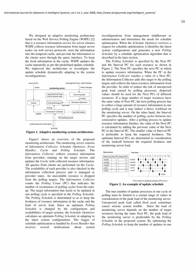
Figure1 shows an overview of the proposed

monitoring architecture. The monitoring server consists

of Information Collector, Schedule Optimizer, Event

Handler, Cache and Polling Schedule. The

Information Collector collects resource information

from providers running on the target servers and

updates the Cache with collected resource information.

All queries from clients are performed on the Cache.

The availability of each provider is also checked in the

information collection process and is managed as

provider states. An unavailable resource is dropped

from the polling targets. The Information Collector

counts the Polling Count (PC) that indicates the

number of occurrences of polling cycles from the start-

up. The target information that needs to be updated in

one polling cycle is specified in the Polling Schedule.

The Polling Schedule is determined so as to keep the

freshness of resource information in the cache and the

limit of server load. Since an optimum Polling

Schedule is changed by the configuration and

availabilities of target systems, the Schedule Optimizer

calculates an optimum Polling Schedule in adapting to

the latest system configurations. The trigger of

schedule optimization is handled by Event Handler that

receives several notifications about system

reconfigurations from management middleware or

administrators and determines the needs for schedule

optimization. When the Schedule Optimizer receives a

request for schedule optimization, it identifies the latest

system configurations and generates a new Polling

Schedule by a schedule optimization algorithm that is

described in the later section.

The Polling Schedule is specified by the Next PC

and the Interval PC for each resource as shown in

Figure 2. The Next PC specifies the next PC at which

to update resource information. When the PC in the

Information Collector reaches a value of a Next PC,

the Information Collector adds this target to the polling

targets and collects the latest resource information from

the provider. In order to reduce the risk of unexpected

peak load caused by polling processes, dispersed

values should be used for the Next PCs of different

resources. If a large number of target resources have

the same value of Next PC, the next polling process has

to collect a large amount of resource information in one

polling cycle and it may induce a heavy workload on

the monitoring server. On the other hand, the Interval

PC specifies the number of polling cycles between two

consecutive updates. After a polling process to update

resource information finishes, the value of the Next PC

is calculated by adding the previous value of the Next

PC to the Interval PC. The smaller value of Interval PC

is preferable to keep the required freshness. The

optimum Interval PCs are determined in consideration

of the tradeoff between the required freshness and

monitoring server load.

Update

host01 1 3

host02 2 3

host03 3 3

vm01 1 5

vm02 2 5

Next PC Interval PC PC1 2 3 4 5 6 7 8 9 10 11 12

host01

host02

host03

vm01

vm02

Time chartData structure

Resource

The number of update processes at PC=6 is 2 Figure 2. An example of update schedule

The max number of update processes in one cycle of

polling must be limited to a certain range of values in

consideration of the peak load of the monitoring server.

Unexpected peak load called flush peak sometimes

causes serious system trouble. Since the load of

monitoring server depends on the number of target

resources having the same Next PC, the peak load of

the monitoring server is predictable by the Polling

Schedule in the proposed system. By optimizing the

Polling Schedule to keep the number of updates in one

14


polling cycle in a certain level, we can avoid the risk of

the flush peak.

monitoring targets

Monitoring Profile

Gold 2 sec 5 sec

Silver 2 sec 10 sec

Bronze 5 sec 15 sec

lower limit upper limit Profile

Gold Silver Bronze

MonitoringServer

required TTL 3 s 3 s 7 s 7 s 8 s 11 s 13 s 13 s

Figure 3. Monitoring profile to group resources

The monitoring profile figured in Figure 3 is

introduced for grouping the target resources that have

the same class of quality level. As the quality of the

resource information, the freshness is specified by the

TTL in detail. TTL indicates the elapsed time from

data generation. The monitoring profile defines the

lower limit and the upper limit of the update interval.

Since a monitoring profile corresponds to a specific

quality level, system administrator create a new

monitoring profile when a new quality level is required.

Each resource is assigned a monitoring profile and

does not belong to the multiple monitoring profiles.

Administrators simply manage the allocation of each

resource to the specific monitoring profile instead of

editing TTL for each resource. By using monitoring

profile, the operation for the target addition and the

change of monitoring frequency becomes much easier.

3.2. Schedule Generation Problem

The method to generate an optimal polling schedule

is an essential part of the adaptive monitoring system.

The polling schedule has to satisfy the required

freshness of resource information and minimize the

number of concurrent updates.

First, the Interval PC for each resource ri is decided

by the allocated monitoring profile p and the current

polling interval tpoll. The minimum integer j that

satisfies the limits defined in the profile is chosen as

Interval PC. The Interval PC is expressed as the

following expression:

ULLL,|min)(IntervalPC poll ppijtjjr ≤⋅≤∈= N

(1)

where LLp is the lower limit of the update interval for

monitoring profile p and ULp is the upper limit of that.

If any possible values are not found, the

administrator should modify the monitoring profile or

the polling interval to get a possible Interval PC.

Meanwhile, the limited number of concurrent updates

(LCU) in a polling cycle is decided in consideration to

the acceptable load of the monitoring server.

Next, the Next PC for each resource is decided so

that the number of the concurrent updates is not over

the LCU. The number of the concurrent updates is

changed by each PC and the way to set the Next PC.

Since the update processes are executed repeatedly

according to each Interval PC, the change in the

number of the concurrent updates appears with a period

of the least common multiple of Interval PCs (LCMI).

We define the polling schedule generation problem as

follows.

Problem: Polling Schedule Generation

For each resource information ri, the update interval

PC is defined as IntervalPC(ri)

N. Solve the

NextPC(ri)

N for all ri, so that the number of

concurrent updates is under the LCU at any k from 1 to

LCMI.

Solve: )(NextPC, iri∀

Where:

LCU),(U),LCMI1(1

≤≤≤∀ ∑=

n

i

irkkk (2)

≡−

=otherwise0

))(IntervalPC(mod0)(NextPC1),(U

ii

i

rrkrk

(3)

)(IntervalPC)(NextPC1 ii rr ≤≤ (4)

The schedule generation problem is an integer

programming of NextPC(ri), that is classified as NP-

hard. It takes exponential time of the number of targets

“n” to decide if any possible schedule exists or not. If

there are a large number of targets in the system, the

above problem cannot be solved in practical time.

3.3. Schedule Generation Algorithm

To solve the schedule generation problem in

practical time, we propose an algorithm by using an

approximate method.

Algorithm 1:

1) Make groups that have the same value of

IntervalPC(ri).

)(IntervalPC| jrrG iij == (5)

Define J as a set of possible values as j.

15


2) For each group, generate schedule that minimizes

the concurrent updates. Label all ri in Gj as ri,k

)1( jGk ≤≤ and set the NextPC(ri,k) based on this

label.

))( IntervalPC(mod)( NextPC , iki rkr = (6)

The number of max concurrent updates for Gj

is calculated by:

j

G j

3) Combine all generated schedules and calculate

sum of the number of concurrent updates.

∑∈

Jj

j

j

G (7)

Compare the sum of the number of concurrent

updates to the LCU. If the sum of the number of

concurrent updates is smaller than LCU, output

the generated schedule as a possible schedule.

Otherwise, give up the schedule generation.

Algorithm 1 divides the all ri into the groups that

have the same value of IntervalPC(ri) and solves the

partial optimal schedule for each group. By gathering

the partial schedules, the max number of concurrent

updates is minimized in most situations. Furthermore,

the algorithm always outputs a result in O(n) time.

If each pair of IntervalPC(ri)s of the different

groups is relatively prime, the Algorithm 1 always

solves the optimal schedule (i.e. minimize the number

of the concurrent updates) by the following theorems.

Theorem 1:

When all of the IntervalPC(ri) have the same value,

the max number of the concurrent updates of the

schedule is equal to or more than

)(IntervalPC ir

n ,

where n is the number of targets.

Proof 1:

Let α be the max number of the concurrent

updates. All of ri have to be updated during

IntervalPC(ri) within α update processes.

)(IntervalPC irn ⋅≤ α (8)

Because α is an integer value, the following condition

is obtained.

≥

)(IntervalPC ir

nα

(9)

Theorem 2:

Gp and Gq are groups of resource information that

has intervals of p and q. If p is coprime to q, the max

number of the concurrent updates of the update

schedule for all elements of Gp and Gq is equal to or

more than

+

q

G

p

G qp .

Proof 2:

For any rp1 ∈ Gp and any rq1 ∈ Gq, the PC to

update: tp(rp1) and tq (rq1) are generally represented by:

)(NextPC)( 11 pppprpmrt +⋅= (10)

)(NextPC)( 11 qqqq rqmrt +⋅= (11)

where, mp and mq are any positive integer values.

Here, for any NextPC(rp1) and any NextPC(rq1),

there exists a pair of mp and mq satisfying tp(rp1) = tq

(rq1) modulo pq. This is derived from the Chinese

remainder theorem [6].

Therefore, there exists a case where the number of

concurrent updates is 2 for any pair of rp1 and rq1. The

max number of the concurrent updates, α , is given by:

qp ααα += (12)

where pα and

qα are the max number of the

concurrent updates for Gp and Gq.

From the Theorem 1, the following condition is

obtained.

+

≥

q

G

p

G qpα

(13)

Because the max number of the concurrent updates

of the schedule generated by the Algorithm 1 is

∑∈

Jj

j

j

G , the output schedule is always optimal if each

pair of IntervalPC(ri)s of the different groups is

relatively prime.

4. Evaluation

This section describes the experimental evaluations

of the proposed adaptive monitoring system using a

system reconfiguration scenario.

4.1. Monitoring load estimation

The load of the monitoring server such as CPU

usage and the amount of the network traffic depends on

the number of concurrent update processes. By

investigating the relationship between the load of the

monitoring server and the number of the concurrent

updates, the load of the monitoring server at real

16


y = 0.5336x + 1.5633R² = 0.9989

0

1

2

3

4

5

6

7

0 1 2 3 4 5 6 7 8

Avera

ge C

PU

usag

e (%

)

Number of concurrent updates

y = 0.6471x + 3.0902R² = 0.9935

0

1

2

3

4

5

6

7

8

9

0 1 2 3 4 5 6 7 8

Max C

PU

usag

e (%

)


y = 24.44x + 1.8874R² = 0.9997

0

50

100

150

200

250

0 1 2 3 4 5 6 7 8

Avera

ge T

ran

mis

sio

n (K

bp

s)


y = 34.757x + 6.4035R² = 0.999

0

50

100

150

200

250

300

0 1 2 3 4 5 6 7 8

Max T

ran

mis

sio

n (K

bp

s)


(a) Average CPU usage (b) Max CPU usage (c) Average NW Transmission (d) Max NW Transmission

Figure 4. The relationship between the number of concurrent updates and the monitoring loads

execution can be estimated from the installed polling

schedule.

The experimental environment has a monitoring

server that has 3GHz Intel Pentium4 processor and 2.3

GB of RAM. On this server, WSPE collects resource

information from several physical and virtual machines.

Each target provides 12 KB of resource information.

All nodes used in the experiments are connected by

100 Mbps ethernet.

In this testing environment, we measured several

system metrics like CPU usages, memory usages, disk

I/O and network traffics by varying the number of

concurrent updates. The relationship between the

system metrics and the number of concurrent updates

can be characterized by regression analysis. Figure 4

(a) shows the plots of the measured values of CPU

usages under the limited number of the concurrent

updates. The relationship is expressed as the following

expression by applying the least square method to the

observed values.

5633.15336.0 +⋅= xy (14)

where x is the number of concurrent updates in a

polling cycle and y is the average CPU usage. The

regression coefficients change depending on the

resource capacities and states of usage. For example,

the more CPU power the monitoring server can use, the

smaller value the gradient of the regression line for the

CPU usage. As far as this experimental environment is

used, the average CPU usage of the monitoring server

is predictable by the obtained regression formula. In

addition to the average CPU usage, the max CPU usage,

the average and max network transmission traffic also

have the linear relation with the number of concurrent

updates (see Figure 4). The other performance data

such as network receive traffic, memory usage and disk

I/O does not have linear relationship with the number

of concurrent updates in our testing environment. From

the results of this investigation, we can find an

appropriate value of the number of concurrent updates

to keep the load of monitoring server in a certain level.

4.2. Adaptation to system reconfigurations

vm01

hostA1

vm02

hostA2

hostB1

hostB2

hostB3

hostB4

hostB5

vm01

hostA1

vm02

hostA2

hostB1

hostB2

hostB3

hostB4

hostB5

hostC1

hostC2

hostC3

hostC4

hostC5

hostC6

hostC7

hostC8

hostC9

hostC10

hostC11

hostC12

hostC13

hostC14

hostC15

Step1: Initial state

Step2: Addition of Cluster-C

cluster-A cluster-B

cluster-A cluster-B cluster-C

vm01

hostA1

vm02

hostA2

vm01

hostA1

hostA2

hostC1

hostC2

hostC3

hostC4

hostC5

hostC6

hostC7

hostC8

hostC9

hostC10

hostC11

hostC12

hostC13

hostC14

hostC15

hostC1

hostC2

hostC3

hostC4

hostC5

hostC6

hostC7

hostC8

hostC9

hostC10

hostC11

hostC12

hostC13

hostC14

hostC15

vm03

Step3: Removal of Cluster-B

Step4: VM defragmentation on Cluster-A

cluster-A cluster-C

cluster-A cluster-C

Figure 5. VM defragmentation scenario

The monitoring adaptation mechanism was

evaluated by a scenario involving the virtual machine

defragmentation as depicted in Figure 5. The

monitoring setting is automatically changed by the

proposed adaptation mechanism for each step of the

17


scenario. The experimental environment consists of

three different clusters, cluster-A, cluster-B and cluster-

C. The cluster-A is established on the virtualized

environment using Xen 2.0 on Fedora Core 4. Cluster-

B consists of 5 nodes and Cluster-C has 15 nodes.

In the first step of the scenario (step 1), the cluster-

A and the cluster-B are monitored from the monitoring

server running on a management server. In the second

step (step 2), the cluster-C is added to the monitored

target of the monitoring server. In the third step (step 3),

the cluster-B is removed from the monitored target. In

the final step (step 4), the defragmentation of virtual

machines on the cluster-A is performed. The

defragmentation moves the virtual machine instance

vm02 to the hostA1, then merges instances of vm01

and vm02, and finally starts a new virtual machine

instance vm03 in the created resource space on the

hostA2. In this experiment, the merge process simply

stops the vm02 and expands the resource allocation to

vm01.

All physical servers and virtual machines have

corresponding monitoring profiles. Table 1 shows the

four different monitoring profiles used in the

experiments. The polling interval tpoll is set to 1 second

and the value of LCU is set to 8. For each step of the

scenario, the optimization algorithm generates the

optimal update schedule that meets the conditions

specified in monitoring profiles and minimizes the

number of concurrent updates under LCU. The

generated update schedules for each step are shown in

Table 2.

Besides the optimization approach, the simple

polling approach and the without-optimization

approach were also evaluated by this scenario for the

sake of comparison. The simple polling approach

updates all of information at regular intervals like

SNMP polling. The regular interval was set to 10

seconds. The without-optimization approach updates

resource information at specific intervals requested

from each monitoring profile. Although this approach

satisfies the conditions of the monitoring profiles, the

number of concurrent updates is not bounded.

Table 1. Monitoring profiles lower limit upper limit

Platinum 3s 10s

Gold 5s 15s

Silver 7s 20s

Bronze 11s 30s

Table 2. Update schedules for each step

clu

ster

no

de

pro

file

Inter

va

l

PC

Next PC

Step

1

Step

2

Step

3

Step

4

A

hostA1 Platinum 3 1 1 1 1

hostA2 Platinum 3 2 2 2 2

vm01 Bronze 11 1 1 1 1

vm02 Bronze 11 2 2 2

vm03 Bronze 11 2

B

hostB1 Platinum 3 3 3





C

hostC1 Gold 5 1 1 1

hostC2 Gold 5 2 2 2

hostC3 Gold 5 3 3 3

hostC4 Gold 5 4 4 4

hostC5 Gold 5 5 5 5

hostC6 Gold 5 1 1 1

hostC7 Gold 5 2 2 2

hostC8 Gold 5 3 3 3

hostC9 Gold 5 4 4 4

hostC10 Gold 5 5 5 5

hostC11 Silver 7 1 1 1





(a) CPU usage (b) Network Transmissions (c) Network Receives

Figure 6. Variation coefficients of CPU usages and network traffics

18


!"# !"# !"#$ !"#%&'&()&*+,-./0123 456 7 89:;<= ;><<9?@ 456 7 AB> >;C9:9DEC9>?456 7 >;C9:9DEC9>? 5FG 7 89:;<= ;><<9?@5FG7 AB> >;C9:9DEC9>? 5FG 7 >;C9:9DEC 9>?$H

!"# !"# !"#$ !"#I*+J2KL22LMJ*+,-./0123 456 7 89:;<= ;><<9?@ 456 7 AB> >;C9:9DEC9>?456 7 >;C9:9DEC 9>? 5FG 7 89:;<= ;><<9?@5FG7 AB> >;C9:9DEC 9>? 5FG 7 >;C9:9DEC9>?

!"# !"# !"#$ !"#NOPQRST&UV3 456 7 89:;<= ;><<9?@ 456 7 AB> >;C9:9DEC 9>?456 7 >;C9:9DEC9>? 5FG7 89:;<= ;><<9?@5FG 7 AB> >;C9:9DEC9>? 5FG7 >;C9:9DEC9>?(a) CPU usage (b) Network Transmissions (c) Network Receives

Figure 7. Max and average values of CPU usages and network traffics

0

1

2

3

4

5

6

0 1 2 3 4 5 6

es

tim

ate

d v

alu

e (%

)

observed value (%)

4

5

6

7

8

9

10

4 5 6 7 8 9 10

esti

mate

d v

alu

e (

%)

observed value (%)

50

70

90

110

130

150

50 70 90 110 130 150

esti

ma

ted

va

lue

(K

bp

s)

observed value (Kbps)

50

90

130

170

210

250

50 90 130 170 210 250

esti

ma

ted

va

lue

(K

bp

s)

observed value (Kbps)

(a) Average CPU usage (b) Max CPU usage (c) Average NW Transmission (d) Max NW Transmission

Figure 8. Observed values versus estimated values by regression functions

We observed the variation coefficients of CPU

usages and network traffics for each step of the

scenario (see Figure 6). All these variation coefficients

were calculated from the time-series performance data

of three minutes duration in each step. The variation

coefficient of optimization approach is the lowest in

any case and the values do not change significantly

over the steps. Compared to the without-optimization

approach, the variation coefficient of network

transmission traffic is reduced by 80% at step 3 (see

Figure 6 (b)). The results indicate that the proposed

adaptive monitoring system stabilize the load of

monitoring server by optimizing the polling schedule

according to the system reconfigurations.

Meanwhile the max values of CPU usages and

network traffics during the three minutes for each step

are shown in Figure 7. The results provide a study of

risk for flash peak of the resource usage. The

optimization approach can lower down the max values

of CPU usages and the network traffics by dispersing

the update processes over time. Compared to the

without-optimization approach, the max transmission

traffic is reduced by 62% at step3 (see Figure 7 (b)).

The proposed optimization approach reduces the risk

of the flash peak.

Additionally the approximate max values are

predicted by using the regression function described in

Section 4.1. Figure 8 shows the relationship between

the measured values and estimated values. The results

show that the estimation provides a good indicator for

availability of the monitoring server.

5. Scalable adaptive monitoring

In this section, we extend the adaptive monitoring

system to hierarchical configurations. To satisfy the

requirements for TTLs from lots of clients, we propose

an algorithm for multiple schedules generation.

5.1. Requirements for scalable monitoring

Large scale enterprise systems distributed in

multiple locations have thousands of monitoring targets

such as servers, routers, switches and applications. A

single monitoring server is not enough to collect the

resource information from thousands of monitoring

targets from the concern for the load of monitoring

19


server and network. Generally, for such a large-scale

system, multiple monitoring servers are configured

hierarchically to integrate the resource information.

HP's NNM can manage 25000 of devices by organizing

monitoring servers hierarchically. MDS [15] and

Ganglia [16] support hierarchical architecture to

aggregate resource information from thousands of

nodes in the grid environment.

Although the hierarchically architecture improves

the scalability of monitoring systems, the overhead of

multiple monitoring servers degrades the query

performance and freshness of resource information.

Users and applications using the monitored information

require the specific level of the query performance and

information freshness. Configurations for monitoring

servers for satisfying the quality requirements are much

more complex than the case with a single server.

Adaptive monitoring that reduces the manual

operations for monitoring settings after system

reconfiguration is also valuable in the large scale

enterprise systems.

For the large scale enterprise systems, we extend the

WSPE to hierarchical configurations. Each WSPE

handles the event of system reconfigurations and adapts

the polling schedule automatically to the target systems.

By optimizing the polling schedule in each WSPE, all

of requirements are satisfied under the capacity

limitations of monitoring servers.

5.2. Hierarchical configuration of WSPEs

WSPE

cache

schedule

WSPE

cache

schedule

WSPE

cache

schedule

WSPE

cache

schedule

WSPE

cache

schedule

clientclientclient

clientclientclient

clientclientclient

clientclientclient

targets targets targets Figure 9. Hierarchically-configured WSPEs

Figure 9 shows a hierarchical configuration of

WSPEs to collect resource information from widely-

distributed systems. Each WSPE has own polling

schedule to keep the freshness of the resource

information in the cache. Some WSPEs collect

resource information from the other WSPE instead of

collecting directly from the target resources. It reduces

traffics to the target resources and distributes the load

of monitoring servers. Clients query the resource

information to the nearest WSPE that has the target

information in the cache. The query response time is

estimated by the turnaround time from the client to the

nearest WSPE.

The TTL of resource information ri in the query

results depends on the polling intervals of all WSPEs

on the path from the client ch to the target resource ri.

Here we denote the polling interval for resource ri in

the WSPE wj as tpoll(wj, ri). Let Wh,i be the set of

WSPEs on the path from the client ch to the target

resoruce ri. The TTL of resource information ri for the

client ch is bounded as the following expression:

∑∈

+≤

ihjw

ijihih rwtrwctrct,W

poll

1

respTTL ),(),,(),( (15)

where tresp(ch, w1, ri) is the time taken to deliver the

information ri from the nearest WSPE h,iw W1

∈ (see

Figure 10).

ch w1 wj ri

tresp(ch,w1,ri)

treq(ch,w1,ri)

tpoll(wj,ri)

Wh,i

tpoll(w1,ri)

client WSPE WSPE target

Figure 10. Model of hierarchical WSPEs

Let treq(ch, w1, ri) be the time taken to request the query

for ri from ch to w1. The query response time is

expressed as follows:

),,(),,(),,( 1

resp

1

req

1

query ihihih rwctrwctrwct += . (16)

If the tquery(ch, w1, ri) does not meet the required

performance of ch due to the limitations of network

performance or server capacity, an additional

placement of a WSPE near the client improves the

query performance at the expense of the information

freshness.

We assume the number of WSPEs and networks are

given by the requirements for the query response time

of each client and the limitation derived from the

network topology. We discuss the problem of polling

schedule optimization to guarantee the required TTLs

for all clients under the limitations of server loads.

5.3. Multiple Polling Schedules Generation

Polling schedules for all WSPEs need to be

optimized for satisfying the requirements for TTL of

20


resource ri from the client ch: RTTL(ch, ri) under the

limitation of server loads given by the LCU of each

WSPE. For a single WSPE, the Interval PCs are

determined by the formula (1) based on the monitoring

profiles. However, for the hierarchically-configured

WSPEs where many clients request to guarantee the

TTL of resource information, the Interval PCs need to

be determined by considering the requested RTTLs and

polling intervals of other WSPEs.

The problem to solve the polling schedules of

WSPEs under the conditions about RTTLs and LCUs

is defined as follows.

Problem: Multiple Polling Schedules Generation

Solve the IntervalPC(wj, ri) and NextPC(wj, ri) for

each WSPE wj to satisfy all requirements of RTTL(ch,

ri), under the limitations of the number of concurrent

updates LCU(wj).

Solve: ),(NextPC),,(IntervalPC,, ijij rwrwji ∀∀

Where:

),RTTL(),(, TTL ihih rcrcth ≤∀ (17)

)LCU(),,(U,1

j

n

i

ij wrwkk ≤∀ ∑=

(18)

≡−

=otherwise0

)),(IntervalPC(mod0),(NextPC1

),,(U

ijij

ij

rwrwk

rwk

(19)

),(IntervalPC),(NextPC1 ijij rwrw ≤≤ (20)

Constraint (17) states the limitation from the

requirements for RTTL(ch, ri). Constraints (18) and

(19) state the limitation of the LCUs. The problem of

multiple polling schedules generation is an integer

programming and NP-hard as well as the schedule

generation problem discussed in Section 3.2.

5.4. Multiple Schedules Generation Algorithm

We propose an algorithm to generate multiple

polling schedules satisfying the requirements of RTTLs

and the limitations of LCUs for hierarchically-

configured WSPEs. The proposed algorithm generates

polling schedules satisfying the constraints (18) by

applying algorithm 1 for each WSPE and readjusts the

Interval PCs so as to satisfy the constraints (17) by

changing the assignment of monitoring profiles.

Algorithm 2:

1) Generate polling schedules for all wj by applying

algorithm 1 with the default monitoring profiles

and the limitation of LCU that are set in each

WSPE.

2) For all requirements for TTL of resource ri from

the client ch, check if the max value of tTTL(ch, ri)

calculated by (15) is below the RTTL(ch, ri). If all

RTTLs are satisfied, output the schedules and

finish the schedule generation process. Otherwise,

go to the following steps to readjust the polling

schedules.

3) Let wk )W1( ,ihk ≤≤ be the sequence of WSPEs

on the path to the ri from ch. The sequence starts

from w1 that is the nearest WSPE from ch. In the

sequence, search a wk that can readjust schedule

so as to satisfy the requirements of RTTL(ch, ri)

by the following step 4. If the wk that can readjust

schedule is not found by the iteration of step 4,

give up the multiple schedule generation.

4) In the given wk, for resource ri, change the

allocation of profile that satisfies both of the

following conditions.

)(),(-),RTTL(UL

)(),(-),RTTL(LL

pollTTL

pollTTL

iihihp

iihihp

rtrctrc

rtrctrc

+≥

+≤

(21)

where LLp is the lower limit of the update interval

for monitoring profile p and ULp is the upper limit

of that. If any profile p that satisfies the

conditions (21), calculate a new IntervalPC(wj, ri)

by the expression (1) with the new profile and

generate a schedule by the algorithm 1. Repeat

finding the possible profiles until get the schedule

or check all profiles.

Since the algorithm 2 is an approximation algorithm,

it does not always output the multiple polling schedules

even if there is a possible solution. However, the

algorithm can change the polling schedules locally to

satisfy the requirements of RTTL(ch, ri) instead of

globally optimization. The algorithm gives the

advantage to adapt the existing polling schedules to the

change of RTTL(ch, ri). Since the monitoring profiles

are edited by system administrator as necessary, the

number of monitoring profiles is limited. The routine of

step 4 is processed in the finite execution time.

6. Related work

Scalable performance monitoring systems have

been well studied in the context of grid computing. A

white paper summarized and evaluated lots of

presented grid monitoring systems [13]. Some

advanced monitoring systems such as Remos [11] and

Network Weather Service (NWS) [12] have a function

21


to forecast the performance changes. In contrast to

several existing works for the grid monitoring systems,

we focus on the quality of the monitoring service,

namely freshness of resource information, in the large

scale enterprise systems.

The quality of monitoring is important especially in

the grid and autonomic computing. The monitoring

requirements differ across applications hosted on the

server and change over time corresponding to the

system configurations. QMON [4] provides a function

to classify and configure the quality of monitoring

based on service level agreement (SLA). QMON

changes the monitoring configuration dynamically by

using the concept of "monitoring channel". However,

the current QMON does not support the adaptation

mechanism to the target system reconfiguration such as

server addition and deletion.

Although freshness is important for applications

using monitored data, the significant emphasis on the

freshness results in a "flash crowd" caused by

monitoring processes [14]. The monitoring system

must manage the server load to avoid the flash crowd.

Our experimental results show that the flash crowd is

avoidable by the optimized schedule.

For the network management, an efficient polling

technique for SNMP is proposed [5]. This technique

provides a function to minimize the polling queries to

the SNMP agents by using the usage parameters

defined by the applications. However, any method to

avoid the flash crowd is not supported.

The necessity of the polling optimization is also

described in the grid monitoring system using slacker

coherence model [3]. The slacker coherence model is

useful to minimize the polling with consideration to the

out-of-sync period of the data. Although this model

considers the load of the target nodes, the server-side

load is not considered. Therefore, there is no guarantee

that the flash crowd does not occur.

7. Conclusion

This paper proposed the adaptive monitoring system

to reduce the administrative operations in the large-

scale enterprise systems. The monitoring server

guarantees the freshness of resource information in the

cache by the polling based cache updates. The update

processes are scheduled to satisfy the requirements of

freshness and the limitation of monitoring server load.

We presented a schedule generation algorithm and

proved that the algorithm generates an optimal

schedule minimizing the max number of concurrent

updates. From the experimental results, the variation

coefficients of CPU usages and network traffics are

improved by at most 80%, and the max values at the

load peak are decreased by at most 62%. The results

show that the proposed method can stabilize the load of

monitoring server and can reduce the risk of flash peak

according to the current system configuration. We

presented as well the extension of the adaptive

monitoring system to be scalable with the algorithm for

generating multiple polling schedules. By applying the

proposed algorithm to hierarchically-configured

WSPEs, we can guarantee all requirements for

freshness of resource information from multiple users

under the limited loads of monitoring servers.

References [1] F. Machida, M. Kawato and Y. Maeno, Adaptive

Monitoring for Virtual Machine Based Reconfigurable Enterprise Systems, 3rd International Conference on Autonomic and Autonomous Systems (ICAS2007), 2007.

[2] F. Machida, M. Kawato and Y. Maeno, Guarantee of Freshness in Resource Information Cache on WSPE: Web Service Polling Engine, 6th IEEE International Symposium on Cluster Computing and the Grid (CCGrid2006), 2006.

[3] R. Sundaresan, M. Lauria, T. Kurc, S. Parthasarathy and Joel Saltz, Adaptive Polling of Grid Resource Monitors Using a Slacker Coherence Model, 12th IEEE International Symposium on High Performance Distributed Computing (HPDC03), 2003.

[4] S. Agarwala, Y. Chen, D. Milojicic and K. Schwan, QMON: QoS- and Utility-Aware Monitoring in Enterprise systems, 3rd IEEE International Cofference on Autonomic Computing (ICAC2006), 2006.

[5] M. Cheikhrouhou and J. Labetoulle, An Efficient Polling Layer for SNMP, IEEE/IFIP Network Operations and Management Symposium (NOMS2000), 2000.

[6] D. E. Knuth, The Art of Computer Programming, Volume 2: Seminumerical Algorithms, 3rd Edition, Section 4.3.2, page 286, Addison-Wesley, 1997.

[7] B. Korte, J. Vygen, Combinatorial Optimization: Theory and Algorithms, Japanese Edition 2005, Section 15.7 NP-Hard Problems, Springer, 2005.

[8] B. Dragovic, K. Fraser, S. Hand, T. Harris, A. Ho, I. Pratt, A. Warfield, P. Barham and R. Neugebauer, Xen and the Art of Virtualization, 19th ACM Symposium on Operating Systems Principles (SOSP19), 2003.

[9] Y. Breitbart, M. Garofalakis, C. Martin, R. Rastogi, S. Seshadri, and A. Silberschatz, Topology discovery in heterogeneous IP networks, 19th Annual Joint Conference of the IEEE Computer and Communications Societies (INFOCOM2000), 2000.

[10] J. Case, M. Fedor, M. Schoffstall and J. Davin, "Simple Network Management Protocol (SNMP)", RFC 1157, 1990.

[11] P. Dinda, T. Gross, R. Karrer, B Lowekamp, N. Miller, P. Steenkiste, and D. Sutherland, The architecture of the remos system. In 10th IEEE International Symposium on High Performance Distributed Computing (HPDC-10), August, 2001.

22


[12] R. Wolski, Experiences with Predicting Resource Performance On-line in Computational Grid Settings, ACM SIGMETRICS Performance Evaluation Review, Volume 30, Number 4, March, 2003, pp 41--49.

[13] M. Gerndt, R. Wismueller, Z. Balaton, G. Gombas, P. Kacsuk, Z. Nemeth, N. Podhorzki, H. Truong, T. Fahringer, M. Bubak, E. Laure and T. Margalef. Performance Tools for the Grid: State of the Art and Future, Automatic Performance Analisis: Real Tools White Paper, 2004.

[14] R. Desai, S. Tilak, B. Gandhi, M. J. Lewis and N. B. Abu-Ghazaleh, Analysis of Query Maching Criteria and Resource Monitoring Models for Grid Application Scheduling, 6th IEEE International Symposium on Cluster Computing and the Grid (CCGrid2006), 2006.

[15] K. Czajkowski, S. Fitzgerald, I. Foster, and C. Kesselman, Grid Information Services for Distributed Resource Sharing, In Tenth IEEE International Symposium on HighPerformance Distributed Computing (HPDC10), IEEE Press, August 2001.

[16] M. L. Massie, B. N. Chun, and D. E. Culler, The Ganglia Distributed Monitoring System: Design, Implementation, and Experience, Parallel Computing, Vol. 30, Issue 7, July, 2004.

[17] HP OpenView Network Node Manager (NNM): http://h20229.www2.hp.com/products/nnm/index.html

[18] IBM Tivoli NetView: http://www-306.ibm.com/software/tivoli/products/netview/

[19] ZABBIX: http://www.zabbix.org/

[20] OpenNMS: http://www.opennms.org/index.php/Main_Page

[21] Nagios: http://nagios.org/

[22] VMware: http://www.vmware.com/

[23] Microsoft Virtual Center: http://www.microsoft.com/windowsserversystem/virtualserver/

23


Abstract—Social ecosystems are growing across the web and

social trust networks formed within these systems create an extraordinary test-bed to study relation dependant notions such as trust, reputation and belief. In order to capture, model and represent the semantics of trust relationships forming the trust networks, main components of relationships are represented and described using ontologies. This paper investigates how effective design of trust ontologies can improve the structure of trust networks created and implemented within semantic web-driven social institutions and systems. Based on the context of our research, we represent a trust ontology that captures the semantics of the structure of trust networks based on the context of social institutions and ecosystems on semantic web.

Index Terms—Semantic Trust, Trust Networks, Trust Ontology, Semantic Social Networks, Ontology Engineering, Structural Analysis.

I. INTRODUCTION

emantic web is described to be a web of knowledge having properties such as heterogeneity, openness and ubiquity. In such an environment where everyone has the ability to

contribute, trustworthiness of these people and their contributions are of great importance and value. As stressed, trust plays a crucial role in bringing the semantic web to its full potential. A trust network can be seen as a structure capturing metadata on a web of individuals with annotations about their trustworthiness. Considering social network as our context, a trust network can be seen as an overlay above the social network that carries trust annotations of the metadata based on the social network, such as user profiles and information. Social networks are gaining increasing popularity on the web

1Nima Dokoohaki is a PhD candidate at

Department of Electronics, Computer and Software Systems (ECS), School of Information and Communications Technology (ICT), Royal Institute of Technology (KTH), Stockholm, Sweden. Email: [email protected]

2Mihhail Matskin is a professor at Department of Electronics, Computer and Software Systems (ECS), School of Information and Communications Technology (ICT), Royal Institute of Technology (KTH), Stockholm, Sweden and professor II (adjunct professor) at Norwegian University of Science and Technology, (NTNU), Trondheim, Norway. Email: [email protected]

while semantic web and its related technologies, are trying to bring social networks to their next level. Social networks are using the semantic web technologies to merge and integrate the social networking user profiles and information. Such efforts are paving the path toward semantic web-driven social ecosystems. Merging and integrating social networking data and information can be of business value and use to web service consumers as well as to web service providers of social systems and networks. Ontologies, at the core of semantic-web driven technologies lead the evolution of social systems on the web. Describing trust relations and their sub-components using ontologies, creates a methodology and mechanism in order to efficiently design and engineer trust networks. “Structure of a given system is the way by which their components interconnect with no changes in their organization” according to [1]. Determining the structure of a society of agents on a trust network structure within a semantic social system, can help us determine the organizational structure of a system. Having this capability we can determine an organization’s certain factors such as flexibility, change capacity, etc. In this paper we investigate how effective design of trust ontologies can improve the structure of trust networks created and implemented within semantic web-based social systems. To address the efficient design of trust networks on semantic web-driven social systems, we have engineered and analyzed a trust ontology [2]. Our trust ontology is based on the main concept of Relationship, that models the main element of trust networks, and two concepts of Main Properties and AuxiliaryProperties, which model properties of relationships. In order to effectively design an ontology for trust, we have introduced a framework for comparing and evaluating trust ontologies. As an experiment, several ontologies of trust have been evaluated according to our framework. To understand the process of engineering the ontology itself, all phases and steps taken during the process of building our proposed trust ontology have been mentioned in details. As an experiment, we have studied the structure of the trust network to describe how a trust ontology can serve as the framework for engineering efficient and scalable trust networks. Same experiment data have been used to create network of other similar works structure-wise to get a deeper knowledge of the

Effective Design of Trust Ontologies for Improvement in the Structure of Socio-Semantic Trust Networks

Nima Dokoohaki1, Mihhail Matskin2

S

24


network structure with respect to ontology design disciplines. The contents of this paper are organized as follows: following the background study and discussion on related research in section 2, state of art in trust ontologies is presented in section 3, our trust ontology is introduced in the section 4, in section 5 trust networks analysis is presented and discussed. Finally we conclude in section 6 and we discuss the future research in section 7.

II. BACKGROUND Within the context of social semantic systems, there has been an extensive amount of efforts based on both academic and practical approaches in order to design and engineer trust networks, but none of the existing works in the field were designed bearing structural and design issues in mind. In this section we introduce the technologies that we have incorporated and considered in our approach. We divide the foundation of our work into two main topics, namely: semantic social networks and trust. In this section we also give a detailed and thorough overview into each field. Each overview is divided into subsections where each of the substantial topics is further studied and discussed.

A. Socio-Semantic Ecosystems Overview In 1967, Stanley Milgram introduced "Small World Hypothesis" [3], which was published by American Sociologist. Social networks became popular in 1990s. A social network is generically defined as a set of people gathered together through connections or links, according to [5]. Web has become a ground for bringing the notion of society of people into life. A web-driven social network needs to be accessible using a web browser and within this network people should be able to explicitly (or implicitly) state their connections and their links to individuals or group of individuals, according to [21]. Web-based social networks continue to evolve, while what is most important today is that connections on these networks, are not single dimensional anymore and today you can model and state different aspects of relationships, such as trust. In 2005, according to [21], there were 115,000,000 accounts within social networks scattered across about 18 online networking communities. It’s important to consider that not all these accounts correspond to a single individual. Many people have multiple memberships across multiple networks, at the same time. Size of the social networks will continue to grow everyday as people realize the “hidden” values of social networking day by day [8]. This growth will continue in size aspect of web grounded social networks and will not stop and as many have

predicted [7] [8], the so called “email scenario” will take place, where the number of advertisements and SPAM messages will increase so drastically that by some point of time these networks will literally collapse. There is a strong and growing demand for fusion of the data from different social networks on web. Many are interested in sharing their profiles, while others are interested in merging their data from multiple networks. Two main reasons can be stated and discussed here: First and foremost, great amount of this data which is scattered throughout all these sites are not shareable and are inaccessible from other networks. Second, as stated many users have different accounts across different networks and if their data merge, then many of these accounts might become a single account. In addition to individuals and users on the web, social networks have become the target of the businesses and industries. There are many businesses and enterprises which sell packages of social networking capable software to their users. So the value of social networking exceeds beyond the borders of individuals and businesses now. 1) Vision of semantic web-driven social institutions Social metadata fusion, in the form of sharing or integration brings business value to entities living within such ecosystems. The vision of “Semantic Social Network (SSN)” [4], describes the fusion and integration of social data across social networks, located on a web of semantics. This vision is based upon two important dimensions: First, semantic descriptions of social data about people available on the web in public, expressed in a formal metadata language such as XML or RDF, with explicitly described links to other people on same or different networks. Second, semantic references to those descriptions described and stored in a formal metadata language such as RDF or XML [4] [5]. There were several attempts to bring this vision into life. One of the most important and influential ones is FOAF (friend-of-a-friend) project [6]. 2) FOAF and SIOC: bringing the vision into life FOAF project creates an RDF vocabulary for describing people and the relationship between them. In this way it can be used as the "glue" in between semantic web and social ecosystems, according to [10]. As described, current Web communities are distributed all around the web, with no links in between them, according to [11].

25


In order to bring semantics to online communities, SIOC [12] (Semantically-Interlinked Online Communities) tries to create the so called “glue” through SIOC ontology [13] [14]. SIOC aims to enable the integration of Web community information and creates the possibility of describing and presenting the social web of data using RDF. We can think of FOAF as an enabler for describing semantic web of individuals, while SIOC enables describing semantic web of communities of individuals. SIOC utilizes the FOAF vocabulary for expressing personal profile and social networking information [11]. 3) Modeling social networks on semantic web Social Network Analysis (SNA) [15] [16], is the science of studying and analyzing a networked setting and it has been applied to settings of networks of health, innovation, etc. Network analysis provides the theoretical as well as practical background for studying how to analyze the network participation effect on certain grounds such as an individuals or groups behavior. Ontologies can be used to model and capture the structure of formal semantics of social networks. Wennerberg [15] describes how the structure of a network can be modeled using a semantic web ontology. Ontologies model, present and document the concepts and properties of a certain domain. Having the social nature of the networks as the domain of the study, ontologies can capture the concepts of relationships, individuals and their respective properties. Inference mechanism gives ontologies the ability of inferring new information using rules which could be of great importance in social context. A set of existing efforts on modeling social network on the semantic web could be mentioned here. Cantador et al. [17], model a social semantic network by utilizing ontology as a basis for clustering the user profiles in a social networking community. The ontology represents the domain of user’s cognitive patterns, such as interests and preferences. Resulting ontological instances, take the shape of a semantic network of interrelated domain concepts and user profiles. A similar effort [18] uses ontology at the core of a semantic web-enabled application. This ontology generates a social network of users and their interests. Generated ontological networks are used in order to detect and filter the Conflict of Interest (COI) relationships in an academic context, comprising authors and reviewers of papers. In a similar effort with the same context, Mika [19] uses ontologies, in the context of a semantic web-driven application system and Flink [19], for modeling, capturing and visualizing the social network of researchers.

B. Trust overview Being the key to any interaction procedure in human societies, trust has been the subject of studies to many fields of research and science such as sociology and psychology, as well as of course computer science. Because of its importance and significance, trust has been harvested as a field of research in for example decentralized access control, public key certification, reputation systems for peer to peer networks, and mobile ad-hoc networks. Despite the fact that there has been a variety of definitions for trust, there has not been an agreement on a generic definition of trust. Researchers mostly have defined trust, depending on the context and the orientation of the paper they have written or the experiments they have been conducting. As a matter of fact most of these definitions are specific to the context of the work being done. Lack of consensus on generic trust definition makes us realize the importance of having a definition which is context-neutral and general enough to be applied to different fields of research and different contexts. Trust is a complex issue, relating to fairness and straightforwardness, honesty and sincerity of a person or the service this person might offer. Grandison [20] defines the trust in the following manner; “Trust is the firm belief in the competence of an entity to act dependably, securely, and reliably within a specified context”. “Distrust may be a useful concept to specify as a means of revoking previously agreed trust or for environments when entities are trusted, by default, and it is necessary to identify some entities which are not trusted”, according to [20]. Distrust is defined as “the lack of firm belief in the competence of an entity to act dependably, securely and reliably within a specified context” [20] [21]. 1) Trust components, properties and sources Trust is presented in the form a relationship between two parties. These two parties, often individuals or agents representing those individuals, are represented as trustor or source, which is defined to be the entity which seeks trust or trust related operations such as evaluation in other entity, trustee or sink, which is the entity that is trusted or it has been requested for trustworthiness-related evaluation. Trust is seen as having a purpose or a context. For instance, Alice trusts Bob as a doctor, but she might not trust Bob as a car mechanic, adopted from [20] [24]. In addition, a trust relation might also have a trust metric, which can be quantitative or qualitative, characterizing the degree to which the trustor trusts the trustee. This quality or quantity represents the intensity and level of trust. This quality and quantity can be evaluated by using an algorithm or mechanism which derives trust, according to the metric. For instance, Alice might trust

26


Bob as a doctor very much, while she only moderately trusts Martin as a doctor, adopted from [20] [24]. So far we have realized trust as a computational value depicted by a relationship, described inside a specific context and measured by a metric and is evaluated by a mechanism. Some important properties of trust are stated and discussed [20] [24]. For instance, subjectivity (difference in judgments of two people on the same entity’s trustworthiness) or transitivity (If transitive, when Alice trusts Bob and Bob trusts Cherry, Alice will trust Cherry, adopted from [20] [24]). One of the most important subjects of discussion on properties and components of trust is the difference being made between trust in performance and trust in recommendation [20] [24]. First, there is a difference between trust in an entity to perform an action (trust in performance), and trust in an entity to recommend other entities to perform that action (trust in recommendation). This is the distinction between Cherry trusting Bob as a dentist, and Cherry trusting Bob to recommend a good dentist, according to [20] [24]. Another difference is based on existence of recommenders. There is a difference between the trust that is directly observed by trustor from trustee and the trust that is conveyed and inferred from the recommenders’ trust. As a result, this difference can be sampled between Cherry trusting Bob as dentist, resulting from Cherry’s own direct observation and evaluation from Bob, and Cherry trusting Bob as a dentist, based on the fact that she trusts Shawn as a recommender for a good doctor and on the fact that Shawn trusts (and perhaps recommends) Bob to be a good dentist, adopted from [20] [24]. During the observations made by [25], a set of sources of trust are identified, in both atomic (direct trust) and compound (social trust) forms. Trust is the experience gained from an interaction between two individuals. So the actual experience is the source of trust. Considering the experience, or source of trust between two certain persons and individuals, this type of trust can be referred to as inter-individual trust or what is commonly referred to as direct trust, according to [25]. We can consider a setting of individuals across a web or network. If we consider this society of nodes and present the trust in this society and in this setting, then we are dealing with a new type of trust originating from the experiences gathered by a group of nodes or individuals. This new type of trust has its own source, from trust propagation in social settings or networks. This type is called relational trust, social networks driven trust or in simple form, social trust, according to [25].

2) Trust computation in Web of Trust Most of the models proposed for modeling trust on semantic web are more focused on probabilistic views of trust. They model trust using probabilities assigned as labels to the edges of the networks according to specified trust metric. In order to derive and infer trust, edges are traversed and probabilistic trust values are gathered along the edges and using mechanism adopted, the trust value along the trust path will be computed and inferred. This setting is referred to as a Web of Trust. There are two reasons for making web of trust a candidate for adoption to trust in semantic web computation scenarios. First, both systems are open. Second, trust is considered as being transitive in both settings. Web of Trust was a system that was introduced under the context of security and privacy systems, for instance PGP [55]. In this setting everyone can sign each other’s key and act as certificate holder or certificate authority. Openness states the demand and need for metrics. Need for metrics, establishes and proves the relativity and computability of trust. The need for scalable trust metrics has been discussed and studied extensively [51] [52]. When metrics are applied all the links can carry them and trust can be inferred [27]. Under the assumption of trust transitivity and by enforcing metrics, pathways of trust can be formed and web of trust can be crawled and walked [53]. As stated, semantic web is a similar scenario in which each agent that forms a node on a network is connected to other nodes, agents, and these links and connections form a web of trust. In order to allow everyone, represented by an agent, to evaluate the statements of others in this open and heterogeneous environments, mechanisms and algorithms are developed or adopted to allow everyone to infer and evaluate trust in others using the trust metric-labeled links on the networks of trust. 3) Trust networks The work in this field is mostly focused on the mathematical notion and presentation of networks but the amount of the practical work is limited. Most of the works in this field do not consider design of larger infrastructures and ecosystems. Trust networks are described as weighted graph structures with directed edges. The edges in the generated graphs represent connections and relationships between individuals. Watts introduces the properties of a small world network [37]. He describes a model called ß-model [37] in order to model, construct and generate the structure of social systems. Many social systems have used this model within their infrastructure [34] [35] [36] [37] [38] [27]. Golbeck has done an extensive research effort on trust networks on semantic web, [27] [28] [29] [31]. She has constructed an ontology of trust, combining RDF and FOAF vocabulary to describe relationships comprising trust

27


networks. She has created applications on resulting networks of trust based on her ontology. These applications range from email filtering, TrustMail [27] [28], to web-based recommendation systems, FilmTrust [31]. Brondsema and Schamp [10] have created a system called Konfidi [33] that combines a trust network with the PGP Web-of-Trust (WOT). The system implements a metric and mechanism for inferring the trust on the networks formed. The generated network creates trust pathways in between email sender and receiver that can be crawled and using trust mechanism and metric, trust values are inferred [10].

III. EVALUATING TRUST ONTOLOGIES This section gives an overview in some of the most important and influential works in modeling and designing trust ontologies. After giving a state-of-art overview in the observed ontologies, a framework for comparing and evaluating trust ontologies is introduced and the studied approaches are compared accordingly.

A. State-of-art in trust ontologies As introduced earlier, Friend-Of-A-Friend (FOAF) [6] represents a vocabulary and introduces an ontology for describing a web of connected individuals. This ontology can serve as a tool to model and eventually create a network of society of users by describing personal information about each person (realizing the node itself) and by describing personal information regarding a set of users whom the user knows about (realizing the neighbors on the network). Nodes on such a network are identified by their email address and email serves as their unique identification. 1) Golbeck’s trust ontology Jennifer Golbeck [27], introduces an ontology, that creates an important schema which extends FOAF by using foaf:Person, giving the users this possibility to state and represent their trust in individuals they know. Metric used to express trust is a value on the scalar range of 0-9, in which each scale represents a trust level. These levels are set as properties under the domain of foaf:Person. These levels correspond to: Distrusts absolutely, Distrusts highly, Distrusts moderately, Distrusts slightly, Trusts neutrally, Trusts slightly, Trusts Moderately, Trusts highly, Trusts absolutely, according to [27]. Context was introduced as a property of trust. Trust is context-sensitive, as a result meaning and semantics of trust can change depending on the context. This notion is represented in this ontology under general trust or specific trust or topical trust, according to [27].

For instance, Alice might trust Bob greatly on driving cars but might distrust Bob totally on repairing cars, adopted from [27]. In order to depict general trust within Golbeck’s trust ontology, trust ratings (in the form of trustsHighly or trustsModerately) are described as properties in range of a person class under the range of another person. To describe specific trust and topical trust, other sets of properties are introduced. These properties correspond to the nine values above, but are used to represent trust regarding a specific topic (for instance "distrustsAbsolutelyRe," "trustsModeratelyRe," etc), expressing the level of trust regarding a certain topic such as driving or dishwashing. The range of these properties is the "trustsRegarding", which has been defined to combine a person and a topic of trust. The "trustsRegarding" class has two properties: "trustsPerson" presenting the person being trusted (trustor), and "trustsOnSubject" presenting the subject that trust is stated towards, according to [27]. By having this ability we can query for trust about a person on a specific subject and it is possible also to infer trust on result trust network along the edges where given topic creates the connection and we can crawl along these paths to infer the trust value eventually. 2) Toivonen and Denker’s Message and Context Ontology Toivonen and Denker [41], study the trust in the context of communication and messaging. They state that there are many factors which can have immense impact on the honesty and trustworthiness of the messages we send and receive. The context-sensitivity of trust has been realized and taken into account in their work. The work focuses on drastic changes that many issues, namely reputation, credibility, reliability, trustworthiness and honesty could have, and how they affect the progress of establishing and grounding trust, according to [41]. As a result of the work being done, a set of ontologies have been defined to capture context-sensitive messaging and trust. An ontology is developed to capture and denote the role of context-related properties and information. This ontology captures the domain of message communication and exchange and describes how the context information is actually attached to the messages. This ontology is constructed mainly to visualize how trust is related to message and communication. It is important to note that this ontology extends the topical trust ontology of Golbeck [27], introduced earlier, and it relates the notion of trust to communication and messaging context. Basic idea behind this extension is that:” The topic of a message can have impact on its trust level” [27]. As a result, this trust ontology could be seen as an extension to topical trust ontology realizing the fact how trust can be fused within messages exchanged in the context of a communication environment. This concept is modeled and presented using trustsRegarding property. Links and connections between

28


persons are modeled by the Trusts property. Sub-properties of these two relationships conform to trust levels of Golbeck’s ontology [27]. In order to model the relation of trust to the context, the ctxTRUSTS property is used. If we consider the environment of a simple communication setting, we see the sender, receiver and the communication network mediating them. The messages exchanged in between parties always have contexts, attached to them which in turn allow the computation of ctxTRUSTS properties through Trusts and trustsRegarding properties, according to [41]. 3) Proof Markup Language’s trust Ontology Inference web [42] at Stanford University, has built a semantic web-enabled knowledge platform and infrastructure. This platform is designated to help users on the network to exploit the value of semantic web technologies in order to give and get trust ratings to and from resources on the web. This process is referred to as justification of resources. To this end, a language called PML is used. PML [26] (Proof Markup Language) contains a term set for encoding the justifications and is designated to work in a question answering fashion [44]. PML is designated to help software agents to filter the resources on the web of semantics by proof checking them and justifying the credibility of these resources, on behalf of the users. PML ontology contains three sub-ontologies including: provenance ontology, justification ontology and most importantly trust ontology which captures honesty and trustworthiness statements pertaining to resources. The trust ontology [26] is one of the most important components in PML ontology and we briefly describe the structure of this ontology. The approach presented here is modeling close notions of trust and belief and how it affects the credibility of resources on the web. Notions of belief and trust, with respect to their close semantics, have been presented closely in this ontology. Ontology structure presents the trust and belief relations between a source and a sink (which are both realized and presented using agents) with respect to information from document source under investigation by respective agents. The belief relation shows the belief of an agent about the source. The specific belief has a status (e.g. believes, disbelieves, ignorant). The trust relation shows an agent's overall beliefs about information from the specified source. The metric defined for trust and belief is probabilistic and for both elements a value between range of 0 and 1 has been designated.

4) Konfidi’s trust ontology With respect to metrics used for presenting the trust computational values and modeling the mathematical notion of trust, there exist two approaches: presenting a trust metric with discrete values and metrics with continuous values. Brondsema and Schamp [10] model and represent trust and distrust in a similar fashion using continuous values. Having continuous range of values allows easier propagation of trust values, along the edges on the networks, using inference mechanisms. They represent the relationship as the class and main concept of the ontology. Each relation is directed from source (truster) to sink (trustee). Properties of relations are wrapped under the concept of trust item. The most important feature of this work is, like Jennifer Golbeck’s ontology [27], they have incorporated the notion of “Topical trust” in their ontology. It is used as an attribute and property, which allows to state different features and properties of a relationship. Trust topics and trust values are stated as properties of the trust relationship. In order to describe trust relationships, an ontology is presented using RDF, which in turn eases extending the FOAF vocabulary and profiles. Using the RDF properties, and taking into account that relationship can be described using FOAF vocabulary and ontology, then trust relationships can be described using trust ontology. Other technology that has been integrated is WOT [45] [46] (web-of-trust), that is used to describe web-of-trust resources such as key fingerprints, signature and signing capabilities and identity assurance [10] [46]. Ontology’s RDF schema is made of 2 classes or concepts and 5 attributes or properties. As mentioned, the primary concept is Relationship between two people. Like most trust ontologies, there are two properties that are required for every Relationship, and they form the endpoints of every relationship; truster and trusted using FOAF vocabulary, both truster and trusted have foaf:Person objects as their targets. Using WOT vocabulary, FOAF-defined Persons should also contain at least one wot:fingerprint property specifying the PGP, web-of-trust fingerprint of a public key held by the individual the Person refers to. Most importantly, this property serves for two reasons; first assures the identity of these people described on the both ends of relationship, and it also says if one of the people does not hold any keys then system can ignore instantiating a relationship between them.

B. Comparison and analysis In this section we will compare some of the most important afore mentioned ontologies. We will try to point out common and shared points between mentioned ontologies, and we will also try to address strong and weak points among them. Table1 compares the ontologies reviewed so far based on the components of the ontologies.

29


TABLE I COMPARISON AMONG TRUST ONTOLOGIES BASED ON ONTOLOGY COMPONENT STRUCTURE

Trust Ontologies Concept(s) Relationship(s) Instance(s) Axiom(s)

Jennifer Golbeck Topical trust,

Agent,

Person

trustRegarding

(between agent and Topical trust)

trust0...trust10

(range of trust metric),

trustSubject,

trustValue,

trustedAgent,

trustedPerson

(subproperty of trustedAgent),

trustRegarding

“A Person or Agent

(e.g. Alice) trustsHighlyRe (trust10)

trustRegarding a trustedPerson or

trustedAgent (e.g. Bob)

On trustSubject

(e.g. Driving)”

Toivonen,

Denker

Person,

Topic,

Receiver,

Message

Trusts

(between Persons),

ctxTRUSTS

(between receiver and message),

trustsRegarding

(between Person and Topic)

trustRegarding, reTopic,

[trustsAboslutelyRe …

distrustsAbsolutelyRe],

ctxTRUSTS, [ctxtrustsAbosolutely

… ctxdistrustsAboslutely],

trustsRegarding,

Trusts, rePerson,

[trustsAboslutely …

distrustsAboslutely]

Multiple axioms are inferable, for instance;

1) Stating topical trust;

“A Person (Alice) trustsAboslutelyRe

trustsRegarding

(relationship) the Topic (Driving)”,

2) Stating trust between two persons;

“a Person (Alice) trusts another Person (Bob)

trustsAboslutely”

PML Belief

Element,

Trust

Element,

FloatMetric

Belief Relation

(using hasBelievedInformation and hasBelievingAgent

between Agent, information and source),

Trust Relation

(using hasTrustee and

hasTrustor between Agent, information and source)

Agent,

Source,

Information,

hasBelievedInformation,

hasBelievingAgent,

hasTrustee,

hasTrustor,

hasFloatValue,

Two kinds of Axioms regarding the trust and belief

of agent in an information from a source can be inferred, for instance;

2) Stating trust;

“FloatTrust, hasTrustee and hasTrustor

(agent: user’s browser)

And

hasFloatValue

with

FloatMetric (0.55). “

Konfidi Relationship

Item

About

(Between Item and

Relationship)

About,

Truster,

Trusted,

Rating,

Topic,

Trust Relationships can be stated like the following

axiom;

“A

(trust) Relationship

between truster (Alice)

and trusted (Bob)

exists,

which is about

trust topic

(Cooking)

with trust rating

(.95).”

30


To further analyze the study we have done so far let’s consider a set of analysis subjects that affect the discussion on the comparison between ontologies. Depending on the context and the subject of the study certain approaches are used and implemented. If the subject of study is considering ontologies for knowledge management then, it is preferred to use an algorithm to compare ontologies, since such ontologies may be heavy and may contain a large number of concepts and properties. As a matter of fact we can use weight of ontology as the basis of comparison. As all trust ontologies convey the same meaning and that is representation and modeling trust relationship, Context seems to be an important issue. So, we can compare trust ontologies depending on the context they have been modeled and considered in. Since a model should also ease and facilitate the inference and computation of trust, then inference should be also an important topic to consider while analyzing trust ontologies. Trust ontologies are used to generate trust networks and they serve as the gear to rotate the automation of trust network generation, inference and maintenance, therefore we can consider comparing ontologies based on the ease of implementation as well. Ontologies should allow expressivity of trust statements. As axioms represent the trust expressions and statements on the social community of trust, then we can also consider the semantic expressivity of the axioms inferred based on the respective trust ontologies. Semantics of trust should be easy to understand and should allow inference and justifications. The more trust ontologies incorporate and integrate technologies and vocabularies that create expressive and referenced, the more they will be easy to implement. Importing technologies and vocabularies make ontologies rich. As a matter of fact we can also consider basing our justification based on the number or technologies used in an ontology. 1) Weight Considering the size of ontologies, Konfidi is the lightest ontology by having only two main concepts and 5 properties and only one single relationship. PML has 5 main concepts, but there are 2 types of relationship existing with 8 instances, making PML trust ontology the second in the place. While Golbeck’s ontology has one single main concept (topical trust) and two other derived concepts (person and agent), 16 properties and one relationship, making it the third place holder. Trust ontology of Denker/Toivonen has 4 main concepts and 3 types of relationships, making it the heaviest ontological representation of all.

The reason for the excessive size of the number of properties of Golbeck and Denker ontologies, is the trust metric used; if the discrete scale between 0 to 10 was not chosen, and a probabilistic approach was used then the mentioned ontologies would be way lighter, bringing the total number of elements to 11 in Golbeck and to 14 in Denker/Toivonen, make them the top place holders at first and second place. As a matter of fact we can conclude here that the choice of trust metric and the approach toward computational aspect of trust measurement could affect the size of ontology drastically. 2) Context / domain dependence As described context is one of the most important subjects to consider while building a trust model for a domain of study. We also have to consider that there are main elements that affect the construction of trust ontologies that could alter their structure. We want to consider construction of an ontology that could be based on the main axes of trust, semantic web and social network. Considering the main axes and elements that affect the structure of ontology, could create a drastically different ontology with a set of different components. For instance if we consider the trust in service-oriented environments, we have to consider trust as a notion close to security, rather than belief and judgment. In that context trust is more close to reputation, while trust in the context of semantic web and semantic web driven social communities is more close to belief and justification. As a result, context has a considerable impact of the constructing elements of trust ontologies. Among the ontologies considered, Denker/Toivonen is the most context-dependant ontology, as the context of the trust study is communication and message-exchange. Taking a look into trust concepts incorporated into this ontology, we realize that the notion of trust relationship is tangled up in communicational concepts (Communication network, Message) make it completely dependent to communication context although the rest of the trust components are very well-engineered. Since the trust ontology of PML is an axis of a triangle of provenance, justification and trust ontology, all of the mentioned ontologies are incorporated and imported into each other to take advantage of the technical facilities of ontologies description and consumption. This feature makes trust axis of PML ontology, dependent to other three ontologies and incorporating such ontology demands incorporation of the other two ontologies. At the same time this ontology is dedicated to evaluate and express the trust and belief of an agent into a piece of information taken from a source of information on the web. This feature makes it hard to express and conclude the trust between a set of persons, since the other pair should be described by agent as well, but it makes it easy to derive and justify the statements of a person and state the

31


belief and trust in the statement made by a person (for example on a social network). In general, the approach that PML follows is “Trust for Question Answering” [47]. As a result, PML trust ontology seems less context dependant in comparison to Denker/Toivonen and more customizable to the need for modeling trust, in general. While Konfidi makes representation of trust in the context of social semantic networks fairly easy and straightforward, at the same time it is extensible and useful to different contexts and the future needs. Using the Konfidi’s ontology, you can state a statement of topical trust between any set of resources or nodes (described by URI) on a semantic social network. Golbeck’s ontology seems the most essential and fundamental work on describing and stating trust using ontological modeling and representation for the consumption on semantic web. Both Konfidi and Golbeck’s ontologies are among the most context and domain independent ontologies and that makes them easy to be customized and implemented in other domains of interests, demanding for modeling of trust. We can state that the more ontology has components that directly expresses the trust relationships and has less components and properties related to other domains, the more context-independent it will be. 3) Inference capability One of the most important issues while considering capturing of a domain inside the structure of ontology, is the reasoning based on that ontology. Considering the subject of discussion, it should be possible to infer trust values easily using the corresponding trust ontology. As described, choice of trust metric plays a crucial role in the design and composition of ontology. Given a set of entities (for instance two persons located on a network), ontology should facilitate the inference of computational trust value for the given entities. There are certain factors that affect the efficient inference based on ontology such as the complexity and size of trust network generated. The lesser trust network generated is complex the lesser the inference mechanism implemented needs to be complex. Golbeck’s ontology was used for generating a network of semantic data, and was also used within a semantic web social network. Research has shown great inference capability for this ontology [27][28][29][31].Golbeck has studied the inference mechanisms and has created and implemented inference algorithm to study the trust inference based upon her trust ontology on two sets of trust networks, one a website for movie ratings and recommendations [30] and the other for spam filtering [28]. This makes Golbeck’s trust ontology the only ontology widely used, implemented and inferred upon. Konfidi is also tested against network of semantic data, and has shown good performance. Konfidi uses trust strategies to implement different sorts of inference mechanisms and

algorithms, in order to test the inference capability of trust ontology, according to [10]. The inference capability of PML is implemented and has proven to be very effective as it is designated toward automatic resource evaluation. It is important to consider that trust inference capability is an important factor that affects the implementation aspects of trust representation. 4) Semantic expressivity Axioms that are inferred from trust ontologies express the semantics of trust. The more clear and expressive these axioms become the easier they will describe the semantics of trust within the implemented and stated context. Golbeck’s and Konfidi’s respective ontologies state the semantic trust relationships very easy to understand and very expressive; for example using Konfidi; “Relationship between truster (Alice) and trusted (Bob) exists, which is about trust topic (Cooking) with trust rating (.95).” and using the Golbeck’s ontology;” “A Person (Alice) trustsHighlyRe trustRegarding a trustedPerson (Bob) on trustSubject (Driving)”, adopted respectively from [27] [10]. As Denker/Toivonen use Golbeck’s approach, but the axioms generated are less expressive as multiple contexts are taken under consideration and final driven axioms should have the notions of context, trust, communication. Considering all intermediary relationships for example, a trust relationship between person and topic could be described as; “a Person (Alice) rePerson trustsAboslutelyRe (trust metric) trustsRegarding (relationship) reTopic Topic (Driving)”, adopted from [27], which shows less expressivity than previous axioms. As described in the table, PML has the less expressivity among all, but this is traded off with the inference capability of the ontology, as the inference should be consumed by software agents. There seems to be a tradeoff between the expressivity of inference capabilities of ontologies; as the ontology becomes consumable by software agents, the less expressive the inference products become. 5) Size of trust networks We discussed that the trust network should be automatically generated during runtime so we can analyze and evaluate and finally infer and compute the trust values based on the generated network. As the size of the corresponding networks grows, the harder the crawling and walking the trust paths becomes. So, it is important to consider that the network generated could be analyzable and inferable. This has to do directly with the

32


structure based on which trust concepts and properties are presented and described. For example Konfidi describes the topic and rating, as the extra edges on the network tree. The more topics we incorporate the larger the depth of the network generated becomes, so in order to increase the efficiency, authors of Konfidi’s trust ontology state that the extra information attached to edges could be saved separately, according to [10]. As the semantic concept of trust relationship has been described very efficiently (using a small set of necessary elements, e.g. only one main concept), the networks generated are very well-formed. It is logical to state that the efficient design of ontology directly results on the efficient design of the networks generated and used. As our ontology is introduced in next section, we use network size prospect to analyze the networks generated using our own ontology. 6) Vocabularies incorporated As mentioned before, Golbeck’s trust ontology was indeed a milestone in the field of the work being done for representing trust and belief in statements done on a semantic web-driven community and society. She not only introduced a method of representing trust on semantic web and semantic web-powered societies, but she also introduced the notion of topical trust and subjective trust. By enabling the subjective trust we can state and represent how a sink and a source trust each other based on a specific subject and then measure this trust in subject and topic according to a specific trust metric. Most of other works within trust representation on semantic web and semantic web-driven social networks either base their trust model completely or partially on Golbeck’s trust ontology. Denker and Toivonen incorporate the subjective and topical trust as well into their ontology. They also use the trust range of Golbeck for contextual trust and personal trust representation. Konfidi also incorporates the topical trust. Although not standardized, topical or subjective trust is a requirement for any kind of model capturing the trust relationships. All of the studied ontologies take advantage of friend-of-a-friend (foaf) vocabulary. Golbeck and Konfidi use the foaf vocabulary to describe the two sides of trust relationship. PML uses it to describe the agent that assesses and evaluates the information. Among studied ontologies, Konfidi incorporates and integrates the most number of vocabularies and technologies. In addition to foaf and topical trust vocabularies, Konfidi also incorporates relationship vocabulary [48] and it also uses WOT [45] (web of trust) vocabulary. Using the relationship vocabulary leaves space for

adding other new features of trust relationships when needed; such as the date of initiation of trust relationship, terms of relationship, etc. Integrating different vocabularies, enriches the structure of the ontology, reduces the number of ontology components and eases the inference based upon the respective ontology. Considering standardized vocabularies and ontologies, not only reduces the number of elements, but also eases future adoption of new properties of implemented vocabulary-driven features.

IV. ENGINEERING AND CONSTRUCTION OF TRUST ONTOLOGY The same as all engineering sciences, in order to engineer an artifact, an iterative process should be considered where each step proliferates and extends the previous step in the loop to construct the artifact under focus. Ontology engineering and learning is a semi-automatic process, consisting of six main interrelated phases, according to [50] [49]. These phases include: domain understanding, data understanding, task definition, ontology learning, ontology evaluation and refinement with human in the loop, respectively taken from [50] [49]. We use this approach in order to construct and build our trust ontology. We can state that our experience not only can serve as a methodology and mechanism for ontology construction but also, considering the domain of our problem, it can serve as a guide to engineering and construction of trust representations and protocols using ontologies. 1) Determining the domain and scope Considering the domain of problem, we are engineering an ontology, which serves as the representational structure of the relationship visualizing trust and trustworthiness of a set of individuals based on a social network. We can state that this ontology rotates on four main axes; Trust, Relation, Social network, Semantic Web. So, we can state that the domain of our ontology is representation of trust within a social network based on semantic web. 2) Understanding and learning the data Domain and scope of ontology create boundary that captures the data relevant to the ontology under consideration. Since our ontology serves as a representational model, then we understand that the focus will be put on the data that are represented, and that is trust relationships. As relationships are compound data made of couple of atomic subcomponents, then atoms of relationships will form the data of our ontological domain. Relationships are described

33


between entities and these entities are individuals on the social network, connected with trust relationship together. We consider persons on the social network, so data about people will serve as our data. Data about people on the social semantic network are described within FOAF files, which are described using RDF. At the same time Web-of-trust also provides data about the identity of people on our network as well as availability of links between these people on the network of relationships. As such relationships should describe trust as well, properties of trust are also among the pieces of information that are also useful to create data for ontology, such as the measurement and metric value used to describe the value of trustworthiness. In order to be able to describe the subject of the trustworthiness evaluation, we need also a subject list, so, available subjects and topics can be mentioned as available data on the domain. The data needed within this ontology is information that composes trust relationships and properties that relationships have. The main data would be people’s relationships and properties describing them and their relationships; here as mentioned metadata FOAF profiles of people can compose such relationships. 3) Defining tasks Available data describe not only information about people that make the atoms of relationship molecules but also the properties of relationships. When domain is specified and the data available are recognized and learned, usages and functionalities of ontology being constructed is specified. Taking into consideration the domain and scope of ontology, which is representation of trust relationships and the data available that are information about people creating the relationships, we can state that the task of such ontology would be clearly, describing and representing trust relationships. 4) Ontology learning Using the knowledge acquisition and learning capabilities with the help of our construction and development environment, we are able to learn the ontology. As the main component of the ontology is relationship, that represents the connection between entities on the network then relationship itself serves as the main component and concept of this ontology. We can think of relationship as a composite object made of subcomponents that reside within the relationship and describe the properties of relationship. Each relationship describes an edge on the network, this edge exists between a set of nodes. These nodes represent starts and ends of directed edges (of relationship). hasTruster and hasTrustee respectively represent the two important properties of relationship on a network. So far we have learned the elements of relationship on a social network.

Every relationship has a set of main properties, which describe the nature and purpose of relationship. These properties specify the details of trust relation. Each trust relationship has a topic or subject (topical or subjective trust). In order to make trust computable, on any existing edge on the network there should be a value. This value represents the trust metric used for the representation of trust relationship. So, we can consider Value also as a main property of relationship. Now that we have learned the main elements of ontology, it appears most of the trust ontologies share the same components described so far. Relationship described using ontologies have a set of auxiliary properties, as well. Using this component we can put more details on the relationship and we can give it more weight and mass. It is important to realize that only properties that have less importance than main properties, are described using these properties. These properties are used to give more weight to Relationship. Using a separate element for auxiliary properties leaves space for future extensions that are needed to add to the network Trust relationships are context-sensitive. Context describes whether this relationship is described inside a personal network or a business network. By using context, we can make networks of different types. Using this element we can create simple networks and hybrid networks. For instance, simple networks are either a personal network (such as Orkut [56]) or a business network (such as LinkedIn [57]). We can have a relationship in the context of a personal network. We can also have a simple trust relationship in the context of a business network or perhaps a business environment. When the source is from a personal network and is connected to a sink from a business network we have connected two networks of simple type, creating a hybrid network. As a matter of fact context type can give more details about the type of network where this relationship is described in. This auxiliary element gives more details about the type of network the relationship is based upon. Considering the reason that a relationship can be established based upon, we have also incorporated a Goal property describing the reason that a relationship was based upon. A relationship can have a goal that describes why respective relationship is formed. For instance on a social network, usually the goal for establishing a relationship is friendship, or on a business network, it is seeking business partnership. The most important subsidiary and optional property that we have considered in our ontology is having a recommender as the initiator of the trust relationship establishment. hasRecommender is an auxiliary property describing a person on the network that has recommended trustee, or the sink of relationship, to the truster. In other words, we have described notion of “trust in recommendation” in order to shape and form a relationship, initiated from truster, ended up in trustee, based on guarantee of trust recommender. Using such property we can create networks of different strengths; we can have networks of weak links and strong links.

34


A strong link is a relationship based upon the recommendation of an entity. The more recommenders a relationship has, the stronger this relationship become. A weak link is a relationship that has no recommenders. When speaking in terms of trust, in context of information systems, a way of achieving trust is using a recommender. Considering the transitivity property of trust, the trust in recommender is used in certificate authorities to achieve trust in a third-party. We can take advantage of this property in semantic-web driven social networks to create strong paths in order to use them as the path for aggregating and computing trust values along the network. By specifying auxiliary properties we follow two important goals; Adding more details about relations to ontology and giving more meaning and details to specification of relationships, as well as leaving space for adding more elements describing the other aspects of relationships that may be needed in future. 5) Ontology evaluation As ontology development is a semi-automatic approach and demands involvement of both human and machines, in this phase as well as previous phase we take advantage of using an automated tool in order to build and evaluate our ontology. In this phase we build and evaluate the ontology learned in previous phase. By evaluating the ontology, we estimate the quality of the modeled solution to the addressed tasks defined in previous sections.

It is worth mentioning that in most of the phases of ontology engineering the role of human wouldn’t be completely fade and human will participate in almost all of the phases of ontology development. In order to model and describe the elements and components of the ontology we use Protégé3 ontology editor and knowledge acquisition system. Figure 1 visualizes the structure of our trust ontology. As shown our ontology has 3 main concepts or classes that capture the structure of the trust relationships on the networks. Relationship is the main element and concept of our ontology. MainProperties and AuxiliaryProperties are the other main components of our ontology. We have two associations that connect both MainProperties and AuxiliaryProperties to Relationship. These associations are hasMainProperties and hasAuxiliaryProperties. Relationship always has a sink and a source, which we have described here as truster and trustee. Both hasTruster and hasTrustee are defined on the range of foaf:Agent which enables us to describe relationships in the context of semantic social ecosystems. This agent can be a person, an organization or just a software agent. Each Relationship has to have a truster and a trustee and at least one main property. Without these mentioned elements, a relationship is partial and partial relations are undefined using our ontology. In order to ensure having at least these mentioned elements, we have put restrictions on ontology subcomponents. Restriction defines a blank node with restrictions. It refers to the property that is constrained and defines the restriction itself. Cardinality

3 Protégé, http://protege.stanford.edu/

Fig. 1. Structure of our trust ontology, 3 main concepts of trust ontology as well as two edges connecting them together. [2]

35


constraints define how many times the property can be used on an instance of a class. We have minimum, maximum, exact cardinalities. We have used two exact cardinalities on hasTrustee and hasTruster, in order to state having exactly one truster and one trustee for a relationship. We have also used minimum cardinality for hasMainProperties to make sure having at least a topic and a value for each relationship, and since we can have more than one topic to base the relation upon, we have used minimum cardinality (at least). MainProperties element has two main properties; Subject and Value. We have described these two properties using data type properties, in OWL (Web Ontology Language). Subject takes string value. It is recommended that subject taxonomies or topic ontologies be defined, so we can use a common namespace for describing topics and subjects. Each relationship can have multiple main properties, which means it can be about different topics and subjects, but each main property has to have one and only one topic and only one value. For instance in the relationship between Alice and Bob, Alice can completely trust Bob on Driving (Subject=”Driving”, Value=”0.95”), and also can distrust Bob on Cooking completely (Subject=”Cooking”, Value=”0.10”). This constitutes two distinct main properties in relationship between Alice and Bob. But we cannot have multiple subjects and values in the MainProperties of Alice and Bob on Cooking, for example. In order to enforce this property we have put restriction on both properties of value and subject. By using exact cardinality restriction we have enforced having exactly one subject and exactly one value for each item of trust within a relationship. Finally, AuxiliaryProperties concept of domain has 5 properties and also leaves space for more properties whenever needed. AuxiliaryProperties has an object property and 4 data type properties. It has hasRecommender, which is the element describing the strength of relationship and is defined on the range of foaf:agent that lets us to state which node on the network is the recommender for the establishment of this relationship. ContextType is defined as a string data type property that states the context of the trust network, the relationship is based on. Goal of the relationship is also defined using a string data type property. DateBegin and DateEnd are described using Date data-type property. Clearly we don’t need to have restrictions on any single property of AuxiliaryProperties concept. 6) Discussion As modeling trust is the main target of our work, a brief discussion on the notion of trust and how we have modeled the trust in our approach seems necessary. As discussed, trust is a context-sensitive issue. While considering the context of the trust ontology and trust analysis, we realize that this context is a multi-dimensional entity

composed of two substantial and main dimensions; semantic web and social networks. Trust in the domain of social semantic networks, has three relatively close notions such as belief, provenance and justification. Some of these notions have very close and sometimes overlapping meaning to trust. Among mentioned notions, belief seems to be a very close notion to trust. It seems that belief and trust go hand in hand. Discussion on modeling belief has a long background. The work on belief goes back to Willard Van Orman Quine’s “web of belief” [22]. A reminiscent of web of trust is created by [23] and is weaved into semantic web. They define web of belief as following “by cognitively viewing knowledge as individuals’ rational beliefs about the world, individuals share knowledge and form a distributed knowledge network, which is called the web of belief, where rational belief links individuals with world facts and trust interlinks individuals as external information sources.” [23]. In our work, we have only considered modeling trust and distrust. Considering modeling other notions described takes a great effort and deal of modeling, as each one of these mentioned notions demand their own properties and eventually their own ontologies. As a matter of fact, as we have generalized the notion of trust relationship in our approach to Relationship, then we have provided enough space for future extension. We can build belief ontology that can be imported within our trust ontology and certain elements of these ontologies can be shared and consumed whenever needed. Aside from such possibility then there is a need for future research for defining the nature, usage and representation of belief and judgment in semantic social networks. Using our ontology, we can describe trust in other people on the network regarding a certain topic. Taking into account the discussions we had in previous section, what we are describing here is trust in performance. When we state that “Alice trusts Bob regarding Driving”, this means that, “Alice trusts in eventuality of performance of Bob to some extent, when the act of driving is performed”. Trust in performance describes that truster states the trust in the performance of act of trustee, when this act is performed. This trust uses a probabilistic approach to describe trust relationships, so we can say how much someone trusts the other on a range between 0 and 1. For example, as shown previously we can state, Alice trusts Bob completely regarding a topic. This amount of trust is mapped to a floating point value between 0 and 1, so we can state range of 0.9 to 0.99, is a range showing that you completely trust the person you are expressing trustworthiness about. Considering the discrete range of Golbeck’s ontology, which is between trust0 to trust10, then we realize that we are having an implicit mapping from a range of discrete values to

36


a range of concrete values. Choice of trust topic is also considerable for improvement in future works. As we stated, we have modeled Specific Trust and we have clearly eliminated the notion of general trust. It is important to point out that a relationship should have at least a topic. One of the important notions that we can consider discussing here, is distrust. For instance, “Alice distrusts Bob regarding babysitting to some extent (0.65)”, using our ontology it can be also stated like “Alice trusts Bob regarding babysitting to some (complementary) extent (0.35)”, adopted from [27] [10]. As it is clear we have modeled distrust, implicitly. We have assumed that there is a tradeoff between trust and distrust on the same topic. We can also model feelings using our trust model. If we take all of the evaluation values for a relation, and average it, we can derive the amount of feelings between the trustee and truster. We can derive negative or positive feelings. If there are certain number of trust items (or MainProperties; subjects and values) for a relationship, for instance at least 3, we can consider taking average of the values and deriving a general feeling of truster for trustee. For instance, if Alice has low trust values for Bob in all of the subjects in their relationships, then we can state that she has negative feelings for him, or vice versa. Although, there are many certain properties that should be considered that affect feelings of people for each other and trust is only one of them. Therefore, we can state here that more elements are needed to give us this ability to create feelings statements in our ontology. We want to be able to choose two nodes, a source or truster and a sink or a trustee (trusted), and gather trust values on a path between them on the network and eventually compute a value representing the trust of truster in trustee. In order to address this problem; we have made sure that each relationships on the network has a value, and we have introduced recommenders. Our ontology ensures that if there is a relationship (a link on the network) between two nodes, then this link has a value, although this value doesn’t reflect the general trust value of trust between truster and trustee. In addition to using recommenders, we can use our ontology to create a network of recommendation on the network of trust. We can use recommended links for our trust inference. As we described, recommendation can state the strength of an existing link, so we can use such “recommended link” for our inference along the paths. Theoretically, such paths are stronger and can give better values than other paths that do not have recommenders. One of the main challenges in this context is dealing with distrust values, when encountered on the network. Values of distrust drop the aggregated values along the paths on the

network, and there is no certain procedure or methodology to address dealing with this problem.

V. TRUST NETWORK ANALYSIS We begin by analyzing a network of small size. This gives us the ability to easily, visualize and realize the structure of modeled relationships. Then we move to networks of larger size where we introduce two types of trust network structures; hybrid and meshed networks.

A. A small size network Let us begin with the smallest network size, possible; a network of two people, with a single relationship, containing a main property and an auxiliary property. Let us consider modeling following relational semantics for this atomic network: ”Alice trusts bob in driving a lot.” Using our OWL trust schema and ontology, this network will be presented in RDF format as following; <foaf:Person rdf: ID="Alice"/> <foaf:Person rdf:ID="Bob"/> <Relationship rdf:ID="Relationship_Alice_Bob">

<hasTrustee rdf:resource="#Bob"/> <hasTruster rdf:resource="#Alice"/>

<hasMainProperties> <MainProperties rdf:ID="MainProperties_Alice_Bob">

<Subject rdf:datatype="&xsd;string">Driving</Subject> <Value rdf:datatype="&xsd;float">0.95</Value>

</MainProperties> </hasMainProperties>

</Relationship>

B. Hybrid trust networks Here, we will consider 2 groups of people, representing two networks of different contexts. Each group of four people is interrelated and interlinked, forming a simple network. At the same time a set of these people are connected outside of their own local networks, to other foreign network. These relations work as glue connecting networks of different context, creating Hybrid networks. In hybrid network depicted in Figure 3, people located on one network, are shaping a personal context and their goals are more or less establishing friendship relations, while people on the other network are members of a business network, and their goals are establishing business partnerships and relationships and they could be colleagues in an office environment. It is also considerable to think of the business network as a business-value adding network, or a service oriented environment. In that case, then four latter members

37


can be software agents, which can also be described using our ontology.

In order to consider the structure and size of the generated, a circular represeFigure

Figure 4 visualizes the3. Figure 4 is visualized using Welkin

C. The motivation for studying larger networks of trusconsidering real 4 Welkin,

Fig.4. a circular representation of hnodes and 92 edges)

Fig.3. A hybrid network. Two connected networks of a business network. Hybrid networks, contains 8 people and 12 relations. 8 links are interconnections (local), and 4 links are acting as glue (foreign).


In order to consider the structure and size of the generated, a circular represe

igure


Meshed trust networks

The motivation for studying larger networks of trusconsidering real

Welkin,





igure 4.




Welkin, http://simile.mit.edu/welkin/



can be software agents, which can also be described using our





http://simile.mit.edu/welkin/


Fig.3. A hybrid network. Two connected networks of a business network. Hybrid networks, contains 8 people and 12 relations. 8 links are interconnections (local), and 4 links are acting as glue





The motivation for studying larger networks of trusconsidering real-








The motivation for studying larger networks of trus-world scenarios of network formations. Such


Fig.4. a circular representation of h




Figure 4 visualizes the 3. Figure 4 is visualized using Welkin


The motivation for studying larger networks of trusworld scenarios of network formations. Such


Fig.4. a circular representation of h




RDF trust network depicted in F3. Figure 4 is visualized using Welkin




Fig.4. a circular representation of hybri



In order to consider the structure and size of the generated, a circular representation of network is given in



ybrid network subject to study. (Network contains 48



In order to consider the structure and size of the ntation of network is given in



d network subject to study. (Network contains 48




RDF trust network depicted in F3. Figure 4 is visualized using Welkin4






RDF trust network depicted in F4.



Fig.3. A hybrid network. Two connected networks of different contexts; a personal and a business network. Hybrid networks, contains 8 people and 12 relations. 8 links are interconnections (local), and 4 links are acting as glue



RDF trust network depicted in F



different contexts; a personal and a business network. Hybrid networks, contains 8 people and 12 relations. 8 links are interconnections (local), and 4 links are acting as glue connecting two networks






different contexts; a personal and a business network. Hybrid networks, contains 8 people and 12 relations. 8 links are

connecting two networks









In order to consider the structure and size of the network ntation of network is given in







network ntation of network is given in

RDF trust network depicted in Figure

The motivation for studying larger networks of trust, was world scenarios of network formations. Such






igure

t, was world scenarios of network formations. Such






igure

t, was world scenarios of network formations. Such

networks are complex, combined networks of different sizes and different contexts. We call these networks, networks

Meshed networks are considered networks, where every node is

As such, assumption is unrealistic, and there is only a subset of nodes available that are fullwe consider Taking idea from networnetworks are trust networks where each node is at least connected to a the other hand, a fully connected meshed network is a trust network where each node is connected to everyon

Fig. network contains 16 people and 26 relations.

Fig. and 198 edges)


Meshed networks are considered networks, where every node is connected to all other nodes on the network.


Fig. 5network contains 16 people and 26 relations.

Fig. 6and 198 edges)


Meshed networks are considered networks, where every node connected to all other nodes on the network.


5. A partial meshed network madenetwork contains 16 people and 26 relations.

6. A circular representation of meshed partial network. (Network contains 98 nodes and 198 edges)

networks are complex, combined networks of different sizes and different contexts. We call these networks, networks.



A partial meshed network madenetwork contains 16 people and 26 relations.

A circular representation of meshed partial network. (Network contains 98 nodes and 198 edges)

networks are complex, combined networks of different sizes and different contexts. We call these networks,


As such, assumption is unrealistic, and there is only a subset of nodes available that are fullwe consider partial Taking idea from networnetworks are trust networks where each node is at least connected to a the other hand, a fully connected meshed network is a trust network where each node is connected to everyon


A circular representation of meshed partial network. (Network contains 98 nodes



As such, assumption is unrealistic, and there is only a subset of nodes available that are full

partial Taking idea from networnetworks are trust networks where each node is at least connected to a subset of nodes it has data exchange with. On the other hand, a fully connected meshed network is a trust network where each node is connected to everyon






partial Taking idea from networnetworks are trust networks where each node is at least

subset of nodes it has data exchange with. On the other hand, a fully connected meshed network is a trust network where each node is connected to everyon






partial and Taking idea from networnetworks are trust networks where each node is at least







and fully connected meshed networksTaking idea from networking topologies, partial meshed networks are trust networks where each node is at least


A partial meshed network made-up of two connected hybrid networks. Thinetwork contains 16 people and 26 relations.




As such, assumption is unrealistic, and there is only a subset of nodes available that are fully connected to all other nodes,

fully connected meshed networksking topologies, partial meshed

networks are trust networks where each node is at least subset of nodes it has data exchange with. On

the other hand, a fully connected meshed network is a trust network where each node is connected to everyon

up of two connected hybrid networks. Thinetwork contains 16 people and 26 relations.




As such, assumption is unrealistic, and there is only a subset y connected to all other nodes,




up of two connected hybrid networks. Thi































the other hand, a fully connected meshed network is a trust network where each node is connected to everyone.




Meshed networks are considered networks, where every node




the other hand, a fully connected meshed network is a trust e.



networks are complex, combined networks of different sizes and different contexts. We call these networks, Meshed





the other hand, a fully connected meshed network is a trust



networks are complex, combined networks of different sizes Meshed






up of two connected hybrid networks. This


networks are complex, combined networks of different sizes Meshed



fully connected meshed networks. king topologies, partial meshed




38


In the former, inferring trust values between a pair of nodes on the network seems difficult but, finding a path between a set of nodes on the network is guaranteed. Using our ontology, recommendations can find efficient paths on the network. Figure 5 depicts a partial meshed network of people from different contexts and with different goals perhaps, and can be thought of two hybrid networks integrated and merged together. Figure 6 is a visualization of the RDF network for trust network depicted in Figure 5.

VI. STRUCTURAL COMPARISON In order to emphasize the importance structural determination of trust networks, in this section we consider comparing the structure of the trust networks generated based on three different ontologies; our ontology, Golbeck’s and Konfidi’s. In the last subsection we discuss in details the results of comparison. For the sake of comparison, we have divided the experiment datasets into two sizes; small sized networks and large sized networks.

A. Trust networks of small size Based on our structural point of view, Table 2 lists the number of nodes and edges on the compared networks.

As it is clear, in general the nodes and edges on the networks generated using Golbeck’s ontology is quite smaller than networks generated using our ontology and Konfidi’s. At the same time in both cases our network has a smaller number of nodes and edges than Konfidi’s networks, although the difference is not that much.

B. Trust networks of large size We described and defined hybrid and meshed networks. At the same time, we modeled these networks using datasets that to some extent reflect the structure of such networks. The same datasets were also injected into the structure of two other tested ontologies to consider the structure of the resulting trust networks.

Based on our structural point of view, Table 3 lists the number of nodes and edges on the networks.

Table 3a shows the number of nodes and edges on the networks representing the hybrid network. Network generated using Golbeck’s ontology has less nodes and edges than both of ours and Konfidi’s. Although, network generated using our ontology has less number of edges and nodes in comparison to Konfidi’s. Table 3b shows the number of nodes and edges on the networks representing meshed networks. Again, Golbeck’s network has less number of nodes and edges than our network and Konfidi’s network. Our network has greater number of nodes than both, Golbeck’s and Konfidi’s networks, but lesser number of edges than Konfidi’s.

C. Trust networks of larger size We continued our study by modeling and presenting the trust networks of larger sizes. We also expanded our sample partial meshed network and increased the number of people in the networks and their corresponding relationships randomly. The structure of the resulting networks was studied from the perspective of number of edges and nodes, the same structural perspective used for comparison between networks of small and large size. In our experiment we expanded the sample partial meshed network of 16 people and 26 relationships. The number of people and their corresponding relationships were sampled and plotted at each sample increase to reflect the progress of expansion across the network structure. These data were generated using all three ontologies being evaluated. Figure 7, depicts the effect of seamless increase in the size of trust networks of larger size from structural point of view.

TABLE II COMPARISON BETWEEN THE SIZES OF SMALL NETWORKS

Trust Networks

Golbeck Ours Konfidi

Nodes 15 20 22 Edges 28 34 37 c) Networks of 4 people and 4 relationships. (Increase in size)

Trust

Networks Golbeck Ours Konfidi

Nodes 19 28 29 Edges 46 54 58 d) Networks of 4 people and 6 relationships. (Increase in depth)

TABLE III COMPARISON BETWEEN THE SIZES OF LARGE NETWORKS

Trust Networks


Nodes 27 48 50 Edges 73 92 105

a) Hybrid Network (network of 8 people and 12 relationships).

Trust Networks


Nodes 49 98 86 Edges 132 198 211

b) Meshed network (Networks of 16 people and 26 relationships).

39


a) Increasing the size of Golbeck’s trust networks. The diagram depicts the increase in range of nodes and edges, starting from network of 20 people and 18 relations, ending at a network of 108 people and 104 relations.

b) Increasing the size of Konfidi’s trust networks. The diagram depicts the increase in range of nodes and edges, starting from network of 28 people and 32 relations, ending at a network of 96 people and 66 relations.

c) Increasing the size of our trust networks. The diagram depicts the increase in range of nodes and edges, starting from network of 24 people and 20 relations, ending at a network of 112 people and 64 relations.

Fig. 7. Networks of larger sizes: Effect of increasing the number of people on the networks described using different ontological structures.

40


D. Detailed analysis of structural comparisons In this section we further analyze and study the results of our experiment and comparisons. As shown in Tables 1 and 2, trust networks modeled, described and presented using our ontology and others are compared based on the number of nodes and edges (structural perspective). Comparison shows that in networks of small size, our ontology shows average performance in comparison to other ontologies, meaning that trust networks generated have average sizes, in comparison. But as the size of the networks increases, certain aspect of trust network size increases more than other compared network, showing less efficient performance. This decrease in efficient performance is also well-depicted in networks of larger size in Figure 7. There are a set of reasons, which can be stated here. Clearly, the main reason, for size increase in networks, is the number of elements incorporated within the structure of ontology. Golbeck’s ontology uses only one main element, Konfidi uses two main elements, while our ontology uses three main concepts.

The second reason would be efficient design of the ontology. Golbeck’s ontology is indeed, a mile stone in the work on trust in semantic web, from different perspectives.

Her trust schema has a very efficient design. Such design has certain aspects that reduce the size of the networks described using that ontology; first, defining levels of trust (trust0...trust10) and trustRegarding on the range of foaf:agent lets you describe the trust directly as the properties of agents and on the trust network. Such efficiency in design lets you describe relations very easily with lesser elements, as seen in results. Konfidi’s trust ontology has more or less the same structure like our ontology. Our ontology has one more element than Konfidi’s, however we have seen networks of smaller size generated by using our ontology have less complex structures than the ones generated by using Konfidi’s ontology. Figures 9 visualizes the structure of the networks generated using our ontology. The emphasis on the visualizing was put on the gravity of the instances on the network toward their originated main elements. An efficient structure will depict the overall organization of the ecosystem and its sub-ecosystems. Our network shows better clustering of elements among the two other samples.

The third reason is the AuxiliaryProperties element of our ontology. As we incorporated an extensibility element for describing secondary and optional properties, we will incorporate extra nodes and more importantly extra edges into the network. In most of the test data for the comparison section, we have auxiliary property elements with at least one sub-element filled. For instance, when describing hybrid networks, all relationships have AuxiliaryProperties with ContextType property of either simple social network, or simple business network, or hybrid network. It should be mentioned here that none of the other compared ontologies, have any element for describing extra properties; extending Golbeck’s trust ontology seems to be very hard and needs drastic changes because of its architecture, and Konfidi doesn’t have any elements for describing extra properties. Taking into account this information, if we eliminate the AuxiliaryProperties element, then the size of our network becomes even more efficient than both other ontologies, in certain situations.

Fig. 7. A clustered visualization of the structure of a meshed trust network based on Jennifer Golbeck’s ontology. This network contains 49 nodes and 132 edges.

Fig. 8. A clustered visualization of the structure of a meshed trust network based on Konfidi’s trust ontology. This network contains 86 nodes and 211 edges.

Fig. 9. A clustered visualization of the structure of a meshed trust network based on our trust ontology. This network contains 98 nodes and 198 edges.

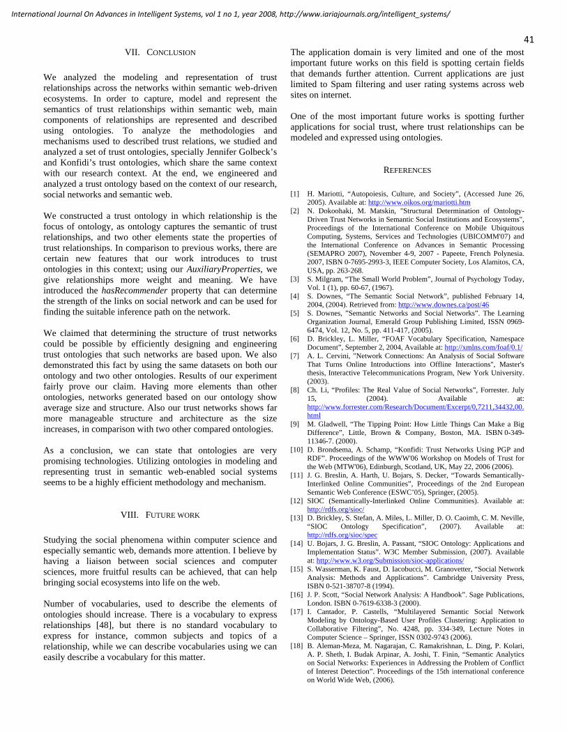
41


VII. CONCLUSION We analyzed the modeling and representation of trust relationships across the networks within semantic web-driven ecosystems. In order to capture, model and represent the semantics of trust relationships within semantic web, main components of relationships are represented and described using ontologies. To analyze the methodologies and mechanisms used to described trust relations, we studied and analyzed a set of trust ontologies, specially Jennifer Golbeck’s and Konfidi’s trust ontologies, which share the same context with our research context. At the end, we engineered and analyzed a trust ontology based on the context of our research, social networks and semantic web. We constructed a trust ontology in which relationship is the focus of ontology, as ontology captures the semantic of trust relationships, and two other elements state the properties of trust relationships. In comparison to previous works, there are certain new features that our work introduces to trust ontologies in this context; using our AuxiliaryProperties, we give relationships more weight and meaning. We have introduced the hasRecommender property that can determine the strength of the links on social network and can be used for finding the suitable inference path on the network. We claimed that determining the structure of trust networks could be possible by efficiently designing and engineering trust ontologies that such networks are based upon. We also demonstrated this fact by using the same datasets on both our ontology and two other ontologies. Results of our experiment fairly prove our claim. Having more elements than other ontologies, networks generated based on our ontology show average size and structure. Also our trust networks shows far more manageable structure and architecture as the size increases, in comparison with two other compared ontologies. As a conclusion, we can state that ontologies are very promising technologies. Utilizing ontologies in modeling and representing trust in semantic web-enabled social systems seems to be a highly efficient methodology and mechanism.

VIII. FUTURE WORK Studying the social phenomena within computer science and especially semantic web, demands more attention. I believe by having a liaison between social sciences and computer sciences, more fruitful results can be achieved, that can help bringing social ecosystems into life on the web. Number of vocabularies, used to describe the elements of ontologies should increase. There is a vocabulary to express relationships [48], but there is no standard vocabulary to express for instance, common subjects and topics of a relationship, while we can describe vocabularies using we can easily describe a vocabulary for this matter.

The application domain is very limited and one of the most important future works on this field is spotting certain fields that demands further attention. Current applications are just limited to Spam filtering and user rating systems across web sites on internet. One of the most important future works is spotting further applications for social trust, where trust relationships can be modeled and expressed using ontologies.

REFERENCES [1] H. Mariotti, “Autopoiesis, Culture, and Society”, (Accessed June 26,

2005). Available at: http://www.oikos.org/mariotti.htm [2] N. Dokoohaki, M. Matskin, "Structural Determination of Ontology-

Driven Trust Networks in Semantic Social Institutions and Ecosystems", Proceedings of the International Conference on Mobile Ubiquitous Computing, Systems, Services and Technologies (UBICOMM'07) and the International Conference on Advances in Semantic Processing (SEMAPRO 2007), November 4-9, 2007 - Papeete, French Polynesia. 2007, ISBN 0-7695-2993-3, IEEE Computer Society, Los Alamitos, CA, USA, pp. 263-268.

[3] S. Milgram, “The Small World Problem”, Journal of Psychology Today, Vol. 1 (1), pp. 60-67, (1967).

[4] S. Downes, “The Semantic Social Network”, published February 14, 2004, (2004). Retrieved from: http://www.downes.ca/post/46

[5] S. Downes, ”Semantic Networks and Social Networks”. The Learning Organization Journal, Emerald Group Publishing Limited, ISSN 0969-6474, Vol. 12, No. 5, pp. 411-417, (2005).

[6] D. Brickley, L. Miller, “FOAF Vocabulary Specification, Namespace Document”, September 2, 2004, Available at: http://xmlns.com/foaf/0.1/

[7] A. L. Cervini, "Network Connections: An Analysis of Social Software That Turns Online Introductions into Offline Interactions", Master's thesis, Interactive Telecommunications Program, New York University. (2003).

[8] Ch. Li, “Profiles: The Real Value of Social Networks”, Forrester. July 15, (2004). Available at: http://www.forrester.com/Research/Document/Excerpt/0,7211,34432,00.html

[9] M. Gladwell, “The Tipping Point: How Little Things Can Make a Big Difference”, Little, Brown & Company, Boston, MA. ISBN 0-349-11346-7. (2000).

[10] D. Brondsema, A. Schamp, “Konfidi: Trust Networks Using PGP and RDF”. Proceedings of the WWW'06 Workshop on Models of Trust for the Web (MTW'06), Edinburgh, Scotland, UK, May 22, 2006 (2006).

[11] J. G. Breslin, A. Harth, U. Bojars, S. Decker, “Towards Semantically-Interlinked Online Communities”, Proceedings of the 2nd European Semantic Web Conference (ESWC’05), Springer, (2005).

[12] SIOC (Semantically-Interlinked Online Communities). Available at: http://rdfs.org/sioc/

[13] D. Brickley, S. Stefan, A. Miles, L. Miller, D. O. Caoimh, C. M. Neville, “SIOC Ontology Specification”, (2007). Available at: http://rdfs.org/sioc/spec

[14] U. Bojars, J. G. Breslin, A. Passant, “SIOC Ontology: Applications and Implementation Status”. W3C Member Submission, (2007). Available at: http://www.w3.org/Submission/sioc-applications/

[15] S. Wasserman, K. Faust, D. Iacobucci, M. Granovetter, “Social Network Analysis: Methods and Applications”. Cambridge University Press, ISBN 0-521-38707-8 (1994).

[16] J. P. Scott, “Social Network Analysis: A Handbook”. Sage Publications, London. ISBN 0-7619-6338-3 (2000).

[17] I. Cantador, P. Castells, “Multilayered Semantic Social Network Modeling by Ontology-Based User Profiles Clustering: Application to Collaborative Filtering”, No. 4248, pp. 334-349, Lecture Notes in Computer Science – Springer, ISSN 0302-9743 (2006).

[18] B. Aleman-Meza, M. Nagarajan, C. Ramakrishnan, L. Ding, P. Kolari, A. P. Sheth, I. Budak Arpinar, A. Joshi, T. Finin, “Semantic Analytics on Social Networks: Experiences in Addressing the Problem of Conflict of Interest Detection”. Proceedings of the 15th international conference on World Wide Web, (2006).

42


[19] P. Mika, “Flink: Semantic Web Technology for the Extraction and Analysis of Social Networks”, Journal of Web Semantics: Science, Services and Agents on the World Wide Web, Vol. 3, No. 2-3, pp. 211-223, (October 2005).

[20] T.W.A. Grandison, “Trust Management for Internet Applications”. PhD thesis, Imperial College of Science, Technology and Medicine, University of London, Department of Computing, (2001).

[21] T.W.A. Grandison, M. Sloman, “A Survey of Trust in Internet Applications”, IEEE Communications Surveys and Tutorials, 1553-877X, Vol.3, No. 4, Page 2, (2000).

[22] W.V.O. Quine, J. S. Ullian, ”The Web of Belief”, Random House, New York, ISBN 0-394-32179-0, (1978).

[23] L. Ding, T. Finin, “Weaving the Web of Belief into the Semantic Web”, Proceedings of the 13th International World Wide Web Conference, (2004).

[24] A. Abdul-Rahman, S. Hailes, “A Distributed Trust Model”. Proceedings of Workshop on New Security Paradigms. (1998).

[25] J. Huang, M.S. Fox, “An Ontology of Trust – Formal Semantics and Transitivity”, Proceedings of the 8th ACM International Conference on Electronic Commerce. Fredericton, New Brunswick, Canada, pp.: 259 – 270, ISBN 1-59593-392-1, (2006).

[26] PML 2 Trust Ontology. Available at: http://iw.stanford.edu/2006/06/pml-trust.owl

[27] J. Golbeck, B. Parsia, J. Hendler, ”Trust Networks on the Semantic Web”, ISSU 2782, pp. 238-249, Lecture Notes in Computer Science – Springer, (2003).

[28] J. Golbeck, J. Hendler, “Accuracy of Metrics for Inferring Trust and Reputation in Semantic Web-based Social Network”, ISSU 3257, pp. 116-131, Lecture Notes in Computer Science – Springer (2004).

[29] J. Golbeck, “Computing and Applying Trust in Web-based Social Networks”, University of Maryland, (2005). Available at: https://drum.umd.edu/dspace/bitstream/1903/2384/1/umi-umd-2244.pdf

[30] J. Golbeck, “Inferring Trust Relationships in Web-based Social Networks”, ACM Transactions on Internet Technology, Vol. 7, No. 1, (2006).

[31] J. Golbeck, “FilmTrust: Movie Recommendations from Semantic Web-based Social Networks”, IEEE Consumer Communications and Networking Conference, (2006).

[32] D.L. McGuiness, P.P. Da Silva, L. Ding, “Proof Markup Language (PML) Primer”, (2005). Available at: http://iw.stanford.edu/2005/wd-pml-primer/

[33] Konfidi, Available at: http://konfidi.org/ [34] G. F. Davis, M. Yoo, W.E. Baker, "The Small World of the American

Corporate Elite", Journal of Strategic Organization, Vol. 1, No. 3, pp.301-326, Springer, August 2003, (2003).

[35] C. C. Foster, A. Rapoport, C. J. Orwant, “A Study of a Large Cociogram: Elimination of Free Parameters”. Behavioral Science, Number 8, pp.56-65. (1963).

[36] M. E. J. Newman, "The Structure of Scientific Collaboration Networks," Proceedings of the National Academy of Sciences; 98: 404 - 409. (2001).

[37] D. Watts, “Small Worlds: The Dynamics of Networks between Order and Randomness”. Princeton, NJ: Princeton University Press, ISBN 0-691-00541-9, (1999).

[38] D. Watts, S. H. Strogatz, "Collective Dynamics of Small-World Networks", Journal of Nature, MacMillan Magazines, London, ISSUE 6684, pp. 440-442, (1998).

[39] M. S. Fox, J. Huang, “Knowledge Provenance: An Approach to Modeling and Maintaining the Evolution and Validity of Knowledge”. 22 May 2003, (2003). Retrieved from: http://www.eil.toronto.edu/km/papers/fox-kp1.pdf

[40] J. Huang, M. S. Fox, "Trust Judgment in Knowledge Provenance," DEXA, pp.524-528, 16th International Workshop on Database and Expert Systems Applications (DEXA'05), (2005).

[41] S. Toivonen, G. Denker, ”The Impact of Context on the Trustworthiness of Communication: An Ontological Approach.”, Workshop on Trust, Security, and Reputation on the Semantic Web, (2004).

[42] J. Hradesky, B. Acrement, ”Elements for Building Trust”. Proceedings of iTrust; A Conference on Trust Management. (1994).

[43] Inference Web, Knowledge Systems AI laboratory, Stanford University. Available at: http://iw.stanford.edu/

[44] D.L. McGuiness, P. P. Da Silva, L. Ding, “Proof Markup Language (PML) Primer”, (2007). Available at: http://inference-web.org/2007/primer/

[45] Web of Trust Vocabulary, Version 0.1. Available at: http://xmlns.com/wot/0.1/

[46] D. Brickley, “WOT RDF Vocabulary”. (2002) [47] I. Zaihrayeu, P. P. Da Silva, D. L. McGuinness, “IWTrust: Improving

User Trust in Answers from the Web”. Proceedings of the 3rd International Conference on Trust Management (iTrust). Lecture Notes in Computer Science - Springer. (2005).

[48] I. Davis, Jr. E. Vitiello, “Relationship: A Vocabulary for Describing Relationships Between People”, RDF Vocabulary Specification. (2005). Retrieved from: http://vocab.org/relationship/rel-vocab-20040308.html

[49] J. Davies, R. Studer, P. Warren, “Semantic Web Technologies: Trends and Research in Ontology-based Systems”. John Wiley & Sons, ISBN 0-470-02596-4. (2006).

[50] J. Brank, M. Grobelnik, D. Mladenic, ”A Survey of Ontology Evaluation Techniques”. Proceedings of the Conference on Data Mining and Data Warehouses (SiKDD 2005), Ljubljana, Slovenia. (2005).

[51] A. Jøsang, S. J. Knapskog, “A Metric for Trusted Systems.” Proceedings of the 21st National Security Conference, NSA, October (1998).

[52] J. Avnet, J. Saia, “Towards Robust and Scalable Trust Metrics”. IEEE International Conference, (2003).

[53] G. Caronni, “Walking the Web of Trust”. Proceedings of IEEE 9th International Workshops on Enabling Technologies Infrastructure for Collaborative Enterprises, (WET ICE), ENABL-00, page 153, ISBN 0-7695-0798-0. (2000)

[54] T. Beth, M. Borcherding, B. Klein, “Valuation of Trust in Open Networks”. In Proceedings of the Third European Symposium on Research in Computer Security, ISSU 875, pp. 3–18. Lecture Notes in Computer Science – Springer, (1994)

[55] PR. Zimmermann, “The Official PGP User's Guide”. MIT Press, ISBN 0-262-74017-6, Cambridge, MA, USA. (1995)

[56] Orkut, http://www.orkut.com/. [57] LinkedIn, http://www.linkedin.com/.

43


On Choosing a Load-Balancing Algorithm for Parallel Systems

with Temporal Constraints

Luís Fernando Orleans1, Geraldo Zimbrão1, Pedro Furtado2

1COPPE, Department of Computer and Systems Engineering Federal University of Rio of Janeiro,Brazil

2CISUC, Department of Informatics Engineering, University of Coimbra, Portugallforleans, [email protected], [email protected]

AbstractA key point in parallel systems design is the way clientsrequests are forwarded and distributed among theservers, trying to obtain the maximum throughput fromthem or, in other words, the load-balancing policy.Although it is a largely studied theme, with wellaccepted solutions, the inclusion of temporal constraints,also denoted as deadlines in this work, to the requestsbrings new complexities to the load-balancing problem:how to distribute the tasks and minimize the miss rate.The experiments describe along this paper attests thatthe workload variability plays a crucial role in thisproblem, pointing the big requests as the most criticalelements. Our results also shows that even dynamicload-balancing algorithms are not able to reach anacceptable miss rate, since they handle both short tasksand big tasks the same way. Hence, we propose a newload-balancing algorithm, called ORBITA, which has arequest identification and classification mechanism andan admission control module as well, restricting thenumber of big tasks within the system. This algorithmoutperforms its competitors, which means that it has abigger rate of tasks that end within the deadline,specially when the system is under high load. Aprototype was also built in order to check thecorrectness of the simulation phase. The experimentswere run against a benchmark tool, TPC-C, and all theresults confirmed the previous assumptions, leading tothe conclusion that it is a good practice to understandthe system's workload in order to minimize the miss rate.

Keywords: load-balancing, parallel processing,deadline, ORBITA

1. Introduction

In parallel request processing systems, several parallelservers compute the incoming requests (or tasks) that aredispatched to them according to a load-balancingalgorithm. Typically, these servers provide no guaranteesabout the response times for the request executions, in aso-called a best-effort approach. In peak situations, withrequests arriving at high rates, this policy can lead to a

scenario where a request takes tens of times longer toexecute than it would take in a less stressed server. Thisway, if the system provides some kind of quality ofservice, such as trying to guarantee that response timeswould not be higher than an acceptable threshold,denoted as deadlines in this paper, the best-effort policycannot be applied. Guaranteeing acceptable responsetimes in parallel processing systems through load-balancing is the main objective of this paper. Ourapproach is meant to be applicable in differentenvironments, including Transaction ProcessingSystems, Web Services, Virtualization Platforms.

This work proposes a new load-balance algorithm,based on the tasks durations (which are supposed to beknown a priori), and our experiments prove that this is abetter approach than blindly dispatching the tasks takingno further considerations as most load-balancealgorithms do. Although there already exists size-awareload-balancing algorithms, such as SITA-E [20], they donot comprise response times concerns, which isresponsible for their poor performance on stressedsystems with deadlined-tasks.

In order to find the best alternative, we have toanalyze the impact of deadlined-tasks and theirvariability in the known load-balancing techniques. Ourapproach is valid and performs better than traditionalload-balancing ones for both hard or soft deadlines.

The simulated architecture comprises only twoservers, because it is the simplest possible parallelarchitecture. This can be easily expanded to n servers aswell and this generalization will be discussed throughoutthe paper.

Figure 1: Simulated architecture

44


2. Related Work

There are plenty of works about load-balancing andQoS, most of them leading to already accepted andconsolidated conclusions. Although these are almostexhausted themes, their combination seems to be an areawhere there are very few research results.

2.1. Load-balancing

Many load-balancing algorithms have been studied,most of them trying to maximize throughput or minimizethe mean response time of requests. Reference [19]proposes an algorithm called TAGS, which is supposedto be the best choice when task sizes are unknown andthey all follow a heavy-tailed distribution. This is not thecase for the scenario analyzed in this paper, in whichtask sizes must be below a deadline threshold. It is alsoshown in [19] that, when task sizes are not heavy-tailed,Least Work Remaining has a higher throughput thenTAGS. In fact, [24] and [23] claim that Least-WorkRemaining is optimal when task sizes are exponentialand unknown.

The algorithm SITA-E [20] has the best performancewhen task sizes are known and heavy-tailed but,otherwise, Least-Work-Remaining presents a betterthroughput.

Our previous work in [25] presented a technique todetermine the best multiprogramming level (MPL)offline. Such concept had been expanded and we proposean algorithm that computes the maximum MPL inruntime.

2.2. Quality-of-Service (QoS)

In real distributed systems, task sizes are heavy-tailed.This means that a very small portion of all tasks areresponsible for half of the load [21]. Most tasks are verysmall and there is a small number of big tasks as well. Inmodels with deadlines, like the one analyzed in thispaper, a similar distribution occurs.

Reference [30] presents a model where the number ofconcurrent requests within the system is restricted. Whenthis number is reached, the subsequent requests areenqueued. But this model has no concern for deadlines orrejection of requests. It also does not show a way to load-balance the arriving tasks, since it is a single-serverarchitecture.

Quality-of-Service was also studied for Web Servers.In [9] the authors propose session-based AdmissionControl (SBAC), noting that longer sessions may resultin purchases and therefore should not be discriminated inoverloaded conditions. They propose self-tunableadmission control based on hybrid or predictivestrategies. Reference [8] uses a rather complex analyticalmodel to perform admission control. There are alsoapproaches proposing some kind of servicedifferentiation: [5] proposes architecture for Web servers

with differentiated services; [6] defines two priorityclasses for requests, with corresponding queues andadmission control over those queues. In [30], the authorspropose an approach for Web Servers to adaptautomatically to changing workload characteristics and[14] proposes a strategy that improves the service torequests using statistical characterization of thoserequests and services.

Comparing to our own work, the load-balancingalternatives referred above do not consider QoSparameters, such as deadlines, and the QoS studiesconcern single server systems, only. Our approach usesmultiple servers and a careful request allocation to thoseservers in order to comply with the deadline constraints.

3. Modelling typical real distributions

In order to analyze and propose time-consideringload-balance approaches, it is important to understandfirst the kinds of workloads distributions that happentypically and how to model them. The typical requestworkload, such as Transaction Processing Systems, isquite heterogeneous in what concerns servicingrequirements.

Besides the algorithm SITA-E, reference [20] presentsa study that claims that the distribution of task sizes (ordurations) in computer applications are not exponential,but heavy-tailed. In short, a heavy-tailed distributionfollows three properties:

1. Decreasing failure rate: the longer a task runs, thelonger it is expected to continue running.

2. Infinite variance3. A very small fraction (< 1%) of the very largest

tasks makes up a large fraction (50%) of the load. Thisproperty is often called as the heavy-tailed property.

The simplest heavy-tailed distribution is the Paretodistribution, with probability mass function:

f x=akaxa1

,a , k0, xk ,

and cumulative distribution function

F x=1k÷ xa .

In these functions, k is the smallest possibleobservation, whereas a is the exponent of the power law,and will be called hereafter as the variance factor of thefunction. It varies from 0 to 2 and the more it is close to0, the greater is the variability.

4. Traditional load-balancing algorithms and

their weakness

Load balancing is a fundamental basic building block

45


for construction of scalable systems with multipleprocessing elements. There are several proposed load-balancing algorithms, but one of the most common inpractice is also one of the simplest ones - Round-Robin(RR). This algorithm produces a static load-balancingfunctionality, as the tasks are distributed round-the-tablewith no further considerations. At the other hand, thealgorithm Least-Work-Remaining (LWR) produces adynamic load-balancing, as the arriving tasks aredispatched to the server with the least utilization (jobs onqueue or concurrent executing tasks). This algorithm isconsidered in this study, as it is supposed to be the bestchoice when tasks durations are not heavy-tailed.According to [19] and [20], the main issue involvingthese algorithms is the absence of a control over bigtasks, mixing inside the same server short (small) andlong (big) tasks. It becomes more evident when tasksdurations are heavy-tailed, with a minuscule fraction ofthe incoming tasks being responsible for half of the load.In fact, both [19] and [20] propose size-awarealgorithms, trying to minimize the effects caused by thebig tasks on the small ones.

We are concerned with guaranteeing specifiedacceptable response time limits. The number ofconcurrent executions (CE) is a crucial variable whendeadlines are involved, because as we increase thenumber of CE we have a larger probability of missing thedeadlines. As we are going to see, this is an issue thataffects mostly systems where tasks durations have a highvariability, which means that the occurrence of big tasksis more usual. When the variability is low, i.e., thenumber of big tasks is near to zero, all algorithms havesimilar performance curves and practically all tasks arecompleted. As performance starts to degrade as thevariability begins to increase, the number of canceledtasks also gets higher, which gives space for a new size-aware load-balance algorithm, On-demand Restrictionfor Big Tasks, or ORBITA in short. The main idea is toseparate the short tasks, which will always be submittedto execution, from the big tasks, which will have theiradmission by a server (or node) dynamically controlled.This way, a node will only admit big tasks that will notmake the other already running big tasks miss theirdeadlines. Otherwise, the big task will be rejected by thenode, as its admittance would lead to further performancedegradation. In an n servers scenario, a task is onlyrejected if none of the n servers is able to handle it.

In the following we describe each load balancingalgorithm we compare considering deadlines andrejection:

4.1. Least-Work-Remaining (LWR)

for each task that arrives: next_server := server_list ->least_utilized send (task, next_server)

4.2. Task Assignment by Guessing Size (TAGS)

In this algorithm, all incoming tasks are dispatched tothe first server. If a task is running for too long, i.e., is abig task, it is killed and restarted from scratch on thesecond server.

for each task that arrives: send (task, first_server) schedule_dispatch_to_second_server(task)

4.3. Size Interval Task Assignment with EqualLoad (SITA-E)

for each task that arrives: if task is a big task server := server_list ->second_server else server := server_list ->first_server send (task, server)

4.4. On-demand Restrictions for Big Tasks(ORBITA)

for each task that arrives: if task is a small task server := server_list ->first_server send(task, server) else server := server_list ->second_server bigger_task := bigger_running_task(server) max_ce := LOWER_BOUND(deadline/bigger_task) if number_of_running_tasks(server) >= max_ce NOT_ADMITT(task) else send (task, server)

Figure 2 depicts how LWR and SITA-E behave. In thefigure, a new job with estimated duration of 3 units oftime (UT) is received (2a) and there are 2servers: one isexecuting 3 short tasks and the other one is executing 2long tasks. If the load-balancer module, the light-grayrectangle in figures, is using a LWR strategy, then thenew task is dispatched to the second server (2b). On theother hand, if a size-aware algorithm (like SITA-E) isused, the job is forwarded to the first server, the onecontaining short tasks (2c).

5. Simulation setup

Due to the large number of parameters involved, itbecomes necessary to formally describe the simulationmodel used in this work. The simulator has the followingparameters :

Number of servers. Tasks arrival rate (follows an exponential

distribution).

46


Task size distribution (follows a Paretodistribution).

Maximum amount of time a task can execute(deadline).

Load-balancing algorithm. Minimum size of big tasks.

In this paper, a system with 2 identical servers wassimulated. The deadline time was set to 20 seconds andthe duration of each request follows a Pareto distribution,where the value of the parameter a varies from 0.1through 0.3, step 0.1, the smallest possible duration is0.001 second (1 millisecond) and the highest duration is10 seconds. In addition, all tasks have the same priority.The concurrency model is linear, which means that atask will take twice longer if it shares the server withanother task, it will take three times longer in case of twoother tasks and so forth.

The simulator implements all the describedalgorithms: TAGS, SITA-E, LWR and ORBITA and taskarrivals follow an exponential distribution, with

varying from 1 to 10, step 1. Finally, the tasks whichhave their durations below 1 second are considered smalltasks. The big tasks are constituted by all the otherdurations. To eliminate the transient phase, the dataobtained in the first hour of the simulation wasdiscarded. Only the results obtained in the next 5 hourswere considered.

5.1. Task duration generation

Since we are simulating a scenario where tasks havedeadlines, the variance is not infinite. But as we areinterested in studying how the system behaves when thenumber of small tasks is much greater than the numberof big tasks, the Pareto distribution is used to generatethe duration of the tasks. The MOD function will beapplied to all durations that exceed the deadline time(generated_duration MOD deadline), in order to equally

distribute them among the allowed durations. Table 1shows the percentage of the generated durations forvalues of a versus the intervals (that must be read as[min, max[). It is to notice that when a assumes lowervalues, the variability is higher. Even in these cases, thenumber of durations within the interval [0,1[ is muchgreater than the others.

5.2. Simulation Results

In these experimental results, we analyze first resultsfor all tasks, showing that ORBITA has better or at leastas good performance as other approaches in that case,and almost zero miss rates unlike the other strategies.The big tasks are a small fraction of the workload, butthey are the ones with the largest miss rates for moststrategies, and that is where ORBITA obtains muchbetter results than the other ones because it considerstime constraints. For this reason we then analyze resultsconcerning the big tasks.

Figure 4a shows the performance of the algorithmswhen tasks durations highly vary. It can be noticed that,as the arrival rate raises, both LWR and TAGS performsworse in comparison with the other two algorithms,SITA-E and ORBITA. This low performance occurs dueto the fact that those algorithms mix small and big tasksinside the same server, while SITA-E and ORBITAreserve a server to execute small, fast requests. A quicklook to figure 5a attests this explanation: LWR andTAGS have small tasks getting canceled, an event thatdoes not occur nor in SITA-E neither in ORBITA. Evena high arrival rate such as 10 tasks per second does notmake the small tasks miss their deadlines when thosealgorithms are used.

If the variance factor was set to 0.3, the throughput ofthe four strategies would be very similar, as shown infigure 4b. As this variance factor generates a smallernumber of big tasks, the assumption that mixing all kind

(a) (b) (c)

Figure 2: A new transaction arrives (a). LWR approach (b). Size-aware approach(c).

3

11

3

983

11

3

98

31

13

98

Table 1: Percentage of generated durations, according to the variance factor (a) of the Paretodistribution and the duration inteval.

a [0, 1[ [1, 2[ [2, 3[ [3, 4[ [4, 5[ [5, 6[ [6, 7[ [7, 8[ [8, 9[ [9, 10[ 10

0,1 53,88% 6,97% 5,17% 4,90% 4,42% 4,64% 3,93% 4,24% 4,25% 3,74% 3,85%

0,2 76,02% 4,75% 3,18% 2,94% 2,30% 1,90% 1,87% 1,95% 1,79% 1,56% 1,75%

0,3 87,90% 2,91% 1,76% 1,38% 1,12% 0,98% 0,89% 0,80% 0,78% 0,75% 0,73%

47


1 2 3 4 5 6 7 8 9 10

0

2

4

6

8

10

12

14

16

LWR

TAGSSITA-E

ORBITA

Arrival Rate

Thro

uhput (T

asks

per

min

ute

)

1 2 3 4 5 6 7 8 9 10

0

2

4

6

8

10

12

14

16

18

20

LWRTAGS

SITA-EORBITA

Arrival Rate

Thro

ughput (T

asks

per

min

ute

)

(a) (b)Figure 3: Throughput of big tasks with variance factor 0.1 (a) and 0.3 (b).

1 2 3 4 5 6 7 8 9 10

0

50

100

150

200

250

300

350

400

LWRTAGS

SITA-EORBITA

Arrival Rate

Thro

ughput (T

asks

per

min

ute

)

1 2 3 4 5 6 7 8 9 10

0

100

200

300

400

500

600

LWR

TAGS

SITA-E

ORBITA

Arrival Rate

Th

rou

gh

pu

t (T

as

ks p

er

min

ute

)

(a) (b)Figure 4: Total throughput with variance factor 0.1 (a) and 0.3 (b).

1 2 3 4 5 6 7 8 9 10

0

10

20

30

40

50

60

LWR

TAGSSITA-E

ORBITA

Arrival Rate

Mis

s R

ate

(Tasks

per

min

ute

)

1 2 3 4 5 6 7 8 9 10

0

50

100

150

200

250

300

LWR

TAGSSITA-E

ORBITA

Arrival Rate

Mis

s R

ate

(Tasks

per

min

ute

)

(a) (b)Figure 5: Throughput of small tasks with variance factor 0.1 (a) and 0.3 (b).

48


of tasks inside the same server for highly heterogeneousworkloads is a bad idea, as shown in figure 4a, isreinforced.

It is worth noticing that in both cases in figure 4, theORBITA algorithm has a better performance than itscompetitors. It becomes more evident if we analyze thethroughput of small tasks and big tasks in separatedgraphics (figures 3 and 5).

As discussed above, both ORBITA and SITA-Epolicies prevent small tasks from being killed. Thisstatement can be observed in figure 5a. A consequence ofthis event is that if we expand the simulated architecturefrom 2 to n parallel servers, only 1 server should besufficient to handle all small tasks, with the other (n-1)servers being used to handle the big tasks. If the arrivalrate keeps growing, there will be a moment when thenumber of servers destinated to handle small tasks shouldalso increase. But the point is that the number of nodesthat should be used to handle big tasks is much morecritical than those that should be dedicated to small tasks.

The graphics shown in figures 3a and 3b shows thethroughput of the big tasks. These pictures confirm therobustness of ORBITA, which maintains the throughputof big tasks almost unaltered, even when the variancefactor is 0.1 and the arrival rate is 10 tasks per second.

Figure 3a shows that, for highly heterogeneousworkloads, ORBITA is the only strategy with satisfactoryresults.

In figure 3b, the algorithm LWR presents a betterthroughput than ORBITA for arrival rates below 7 tasksper second. A closer look at the ended tasks of eachstrategy, displayed in tables 2 and 3, shows that LWRstrategy has a better throughput for task arrival ratescomprehended between 1 and 6, and ORBITA presents abetter throughput for arrival rates higher than 7 tasks per

second. Considering results of figures 3a and 3b together,we conclude that ORBITA is better with highlyheterogeneous workloads or high arrival rates due to itstight control on time constraints. LWR is also aninteresting algorithm as it tries to optimize resourceusage, but does not have enough control over timeconstraints. Our current and future work on this issue,involves considering adaptable ORBITA/LWRalternatives and LWR with time constraints.

6. Prototype experiments

The Midas middleware [29] is a tool that interceptsthe requests sent by an application to a database server. Ituses the Proxy Design Pattern, thus providing atransparent admission control layer, without requiringdeep source code modifications. A simplified class-diagram is shown in figure 6.

The utilization of more than one database serveropens the necessity to keep data synchronized on allnodes, an issue that is known as data replication.According to [35], there are two replication models:eager replication, where the updated data is synchronizedat the other nodes before transaction completion, andlazy replication, where the updated data is sent to otherservers after transaction completion. For simplicity, weused a primary copy replication strategy, since reference[35] attests it is the best choice for eager replication.

7. Experiment Setup

To better understand the implications of ACIDproperties on load-balancing algorithms, we performedvarious rounds of experiments using the TPC-C

Table 3: Throughput histogram of ORBITA algorithm with variance factor 0.3.

[ 0, 1 [ [ 1, 2 [ [ 2, 3 [ [ 3, 4 [ [ 4, 5 [ [ 5, 6 [ [ 6, 7 [ [ 7, 8 [ [ 8, 9 [ [ 9, 10 [ 10

1 53,06 1,43 0,91 0,69 0,53 0,5 0,44 0,41 0,41 0,37 0,37

2 106,07 2,31 1,29 1,11 0,87 0,81 0,64 0,65 0,57 0,55 0,45

3 159,01 2,6 1,38 1,23 1,03 0,97 0,82 0,71 0,68 0,68 0,59

4 211,17 2,92 1,73 1,2 1,05 0,95 0,85 0,8 0,68 0,64 0,65

5 263,86 2,9 1,85 1,24 1,02 1,08 0,86 0,72 0,79 0,65 0,73

6 316,49 3,02 1,75 1,3 1,12 0,94 0,94 0,9 0,71 0,67 0,72

7 370,23 3,21 1,98 1,35 1,11 0,97 0,88 0,75 0,76 0,73 0,71

8 422,01 3,08 1,75 1,47 1,07 1,05 0,9 0,87 0,81 0,7 0,68

9 474,35 3,27 1,98 1,28 1,24 1,08 0,9 0,83 0,74 0,7 0,68

10 529,24 3,13 1,8 1,29 1,11 1,02 0,93 0,91 0,82 0,72 0,68

Arrival Rate

Table 2: Throughput histogram of LWR algorithm with variance factor 0.3.

[ 0, 1 [ [ 1, 2 [ [ 2, 3 [ [ 3, 4 [ [ 4, 5 [ [ 5, 6 [ [ 6, 7 [ [ 7, 8 [ [ 8, 9 [ [ 9, 10 [ 10

1 52,85 1,77 1,09 0,78 0,65 0,5 0,57 0,45 0,41 0,43 0,36

2 106,56 3,62 2,16 1,66 1,39 1,2 0,98 0,97 0,82 0,63 0,58

3 157,52 5,16 3,08 2,54 1,91 1,34 1,15 0,78 0,69 0,46 0,33

4 210,77 7,31 4,4 2,86 1,58 0,96 0,57 0,36 0,25 0,16 0,13

5 264,27 9,19 4,51 1,74 0,7 0,27 0,17 0,09 0,05 0,02 0,02

6 317,21 10,58 3,47 0,79 0,19 0,06 0,02 0,02 0 0 0

7 369,7 11,01 1,63 0,16 0,02 0,01 0 0 0 0 0

8 423,7 9,71 0,56 0,03 0 0 0 0 0 0 0

9 476,46 7,76 0,16 0 0 0 0 0 0 0 0

10 529,75 4,88 0,02 0 0 0 0 0 0 0 0

Arrival Rate

49


benchmark (http://www.tpc.org/tpcc/) in a 2-servers full-replicated database.

Also, to create a more realistic scenario, we modifiedthe workload generation. According to related work [19],typical transactional workloads present high-tailedproperties, which is not the case of TPC-C's defaultworkload. We also made an extra modification on theTPC-C's code, simulating an open model, i.e.,transactions are sent to the system according to astatistical distribution (e.g. an Exponential Distribution).For more informations about open and closed simulationmodels, please refer to [32].

The use of an open model was a bit imprecise due tothe high cost to create and destroy threads (for emulatingclients). For arrival rates greater than 14 transactions persecond, the mean value of the exponential distributionwas not able to be reached. Nevertheless, the obtainedresults clearly simulated high-utilization scenarios, theaim of the experiments.

7.1. Workload Generation

As mentioned before, we used 2 types of transactionmixes: the one described in the TPC-C specification(which we call default transaction mix in this paper) andanother one that aims to reflect a more realistic one, asstated in [19].(denoted here as heavy-tailed transactionmix).

Briefly explaining, the TPC-C specification proposes5 different transactions (in parenthesis are theirfrequency of occurrence): new order (45%), payment(43%), delivery (4%), order status (4%) and stock level(4%). When executing in standalone mode, we found that

new order transaction was the longest one and, incontrast, the stock level was the fastest transaction. So,we create the heavy-tailed transaction mix comprisingonly stock level (95%) and new order (5%) transactions,thus attending the requirements of a heavy-taileddistribution.

To classify transactions in short or long we used amap. As TPC-C has only five different transactions, wecould store pounded mean response times (PMRT) foreach one of them. Hence, each map entry was a pairtransaction name, PMRT. If the PMRT value wasgreater (lower) than a threshold (1 second, arbitrarilychosen) then its corresponding transaction would beclassified as long (short).

A last remark on the workloads: order status and stocklevel transactions are read-only, which means that theyshould not acquire any locks. On the other hand, theothers are update transactions and their isolation levelswere set to Read-Committed.

7.2. Experiments Details

All experiments were executed using a Pentium 43.2GHz, with 2GB RAM DDR2 and a 200 GB SATAHD which was responsible for creating the threads thatsimulate the clients. The servers were 2 Pentium II MMX350MHz, with 256MB RAM and a 60GB IDE HD. Bothservers were running a Debian Linux, with Kernelversion 2.6 and were connected by a full-duplex100Mbps Ethernet link. A PostgreSQL 8.1 databaseserver was running on each server machine and thedatabase size was 1.11GB. The client machine used a

Figure 6: Simplified class-diagram of the Midas middleware.

50


Sun Microsystems' Java Virtual Machine, version 1.5.The database was created with 10 warehouses.

The reason for using the slower computers as thedatabase servers relies on our need to stress the system.Our intention is not to maximize the throughput withindeadline (TWD) the most important metric for thiswork, but to analyze the impact of ACID properties onload-balancing algorithms and their implications on QoSconstraints.

Table 4: Simulation parameters and their values

Parameter Value

Arrival rate Exponential distribution

Simulation time 20 minutes

Warm-up time 5 minutes

Deadline 5 seconds

Finally, each round of experiments was executed for aperiod of 20 minutes. During the first 5 minutes no datawas collected. Before each round, the database wasdropped and then recreated, guaranteeing that all roundsof experiments used the same database state.

7.3. Results

Figures 7 and 8 show the throughput of transactionsthat ended within the deadline versus the arrival rate. Forbest visualization, the results are displayed in terms oflong transactions (a) and short transactions (b).

It can be seen that when the default workload is used(figures 7a and 7b), LWR performs badly. As a result formixing inside the same server both short and longtransactions, only those which are the fastest ones areable to end within the deadline. This can be explained bythe high number of locks obtained by update transactions(the majority on this workload), interfering on theexecution of read-only transactions.

On the other hand, SITA-E and ORBITA performsbetter due to their size-aware nature. Such algorithmsestimate the duration of incoming transactions and, ifclassified as long (short), the transaction is forwarded tothe appropriate server. The thing to be noticed here isthat short transactions are the read-only ones, thus theydo no acquire locks. This explains the high number ofshort transactions that were executed within the deadlinewith these algorithms. On the other hand, the TWD ofupdate transactions is smaller, and for SITA-E it evenpresents a decreasing form on figure 7a. Why doesORBITA perform better than SITA-E? The reason is theadmission control that ORBITA provides for long (big)transactions which are responsible for acquiring locksand, in these cases, for a long period of time. Controllingthe admission of long transactions directly implies incontrolling the number of locks, thus keeping the

accepted transactions ending their executions withintheir deadlines. It can be seen from figure 7a that anarrival rate of 10 transactions per second reaches theoptimal TWD.

A last analysis of figure 7 that is worth mentioning isabout replication. Once all update transactions arereplicated to others servers, why the performance ofsmall transactions was not affected by the replication inSITA-E and ORBITA? The most reasonable answer forthis question relies on the assumption that only the write-set (WS) of update transactions were forwarded to theother server. These WS's do not contain any 'select'statements, thus their execution is also very fast whichmeans that their executions do slow down the read-onlytransaction, but are not capable for making them to miss

their deadlines.Figures 8a and 8b present the performance of the

same algorithms when a heavy-tailed workload is used.One of the properties of such a distribution is massivepresence of short transactions and only a few of very,very big transactions. The results in these figures areinteresting, because the presence of only 5% of new ordertransactions is sufficient to reduce a lot the TWD of shorttransactions when the LWR algorithm was chosen. Infact, when the arrival rate is 6 (which means 360transactions per minute, 95% of them are short), TWDreached its maximum value, about 100. As both servershave to execute new order transactions, locks used by thistransaction (which includes a 'select for update' clause)also occur everywhere. Again, the TWD of longtransactions is zero even for small arrival rates. Thiscan be ironically explained by the massive presence offast transactions, which severely interferes on theexecutions of long transactions. So, long transactions donot permit that the short ones execute within deadline. Inturn, the presence of lots of short transactions areresponsible for the zero-TWD of long jobs.

The other algorithms, SITA-E and ORBITA, havebetter performances. As in the default workload setup,none of the small transactions missed their deadlines,even when data modifications provided by thereplications occur. On the other hand, the execution oflong transactions for SITA-E becomes critical. As thearrival rate increases, the TWD fastly decreases until itreaches zero. Again, the high number of locks areresponsible for the poor performance. In contrast toSITA-E, ORBITA is capable to maintain the TWD oflong transactions in its maximum, due to its admissioncontrol mechanism. A remark about this admissioncontrol relies on the reduced number of long transactionsadmitted. When TWD reached its maximum value, thearrival rate is about 10, what means that 600 transactionsarrives per minute 5% of them (about 30) are of neworder type but only 7 of them were admitted.Otherwise, there might be conflicts on lock acquisitionsand, probably, some transactions (maybe even all ofthem) would miss their deadlines.

51


8. Conclusion and future work

In a parallel system, the incoming tasks must bedispatched to a server according to a load-balancingalgorithm. Most of these algorithms are not aware aboutthe response times of the tasks, since they all follow abest-effort policy. Thus, if tasks arrive at a very high rate,not only fast requests will have to wait for a long periodto be executed, as slower requests will take too long. Inthis paper we propose ORBITA, a load-balancealgorithm that takes time into consideration.

The ORBITA algorithm, which is based on theassumption that tasks durations follow a highlyheterogeneous distribution, differentiates service betweensmall and large requests in order to provide timeguarantees. It was experimentally proved that the bigtasks were the ones responsible for deadline misses, soORBITA works by separating the fast, small tasks fromthe big tasks, which have their admission controlled byeach server. A big task will only be admitted into a server

if it does not make the other running big tasks miss theirdeadlines.

The experiments have shown that when the variabilityof the task durations is high, ORBITA's throughput is notonly greater than the other algorithms, but fairer, sincetasks of all size intervals have low miss rates.

We also implemented a prototype containing threedifferent of the presented load-balancing techniques,each one with different characteristics: Least-Work-Remaining (LWR), Size Interval for Task Assignmentwith Equal Load (SITA-E) and On-Demand Restrictionsfor Big Tasks (ORBITA), our proposal.

Those rounds of experiments were executed in a 2-servers fully replicated database. The dynamic algorithm(LWR) presented the worst performance, since it does notmake differentiations on transactions. Thus, by mixinginside the same server update and read-only transactions,the isolation needed for the first group was responsiblefor making lots of transactions (of both groups) to misstheir deadlines.

2 4 6 8 10 12 14 16 18 20

010

20304050

60708090

100

Arriv al Rate (Transactions per Second)

Tra

ns

acti

ons

per

Min

ute

2 4 6 8 10 12 14 16 18 20

0

10

20

30

40

50

60

70

80

90

LWR

SITA-E

ORBITA

Arrival Rate (Transactions per Second)

Tra

nsa

ctio

ns

per

Min

ute

(a) (b)

Figure 7: Throughputs of long transactions (a) and small transactions (b) when default workload is used.

2 4 6 8 10 12 14 16 18 20

0

1

2

3

4

5

6

7

8


Tra

nsactions p

er

Min

ute

2 4 6 8 10 12 14 16 18 20

0

100

200

300

400

500

600

700

800

900

LWR

SITA-E

ORBITA


Tra

nsactions p

er

Min

ute

(a) (b)

Figure. 8: Throughputs of long transactions (a) and small transactions (b) when heavy-tailed workload is used.

52


On the other hand, the size-aware algorithms (SITA-Eand ORBITA) dynamically recognized read-only(update) transactions and classified them in short (long).This way, each group was assigned to a dedicated server,hence reducing the overall miss rate. Even the replicationcost was not sufficient for deteriorate the performance ofread-only transactions, since only the write-set of thewhole update transaction was forwarded to the otherserver. The main problem for SITA-E relies on theexecution of long transactions, which are responsible foracquiring the locks. The uncontrolled admission ofupdate transactions present in the SITA-E can reduce thenumber of transactions ended within the deadline perminute to zero. In contrast, ORBITA has an admissioncontrol of big transactions. An update transaction is onlyadmitted by the system if it will not cause deadlinemisses from itself or from the other already-runningtransactions.

As future works, we intend to investigate how toeffectively identify and estimate the duration oftransactions. The solution adopted in this paper (using amap with pounded mean response times) was sufficientfor what this work was intended, but we are concerned onif and how to generalize such a concept for a system withad-hoc transactions. We also intend to work on databaseinternals level and study the viability of adding time-constraints mechanisms to queries and/or transactions.

As future work we intend to investigate how ORBITAcan be made to adapt automatically to actual workloadsand arrival rates. This includes how to determine thenumber of servers needed to handle each type of tasks(big and small) and, instead of dividing tasks into twoclasses statically, how to determine and manage taskclasses automatically. We also intend to work on a time-constrained version of LWR and compare theapproaches.

References

[1] Akal, F. et al (2005), Fine-Grained Replication andScheduling with Freshness and Correctness Guarantees.31st Very Large Databases Conference, p. 565 576,Trondheim, Norway, 2005.

[2] Amza, C., Cox, A.L., Zwaenepoel, W. (2005), AComparative Evalution of Transparent ScalingTechniques for Dynamic Content Servers. 21stInternational Conference On Data Engineering, 2005.

[3] Barker, K. et al (2004), A Load-BalancingFramework for Adaptative and AsynchronousApplications, IEEE Journal Transactions on Parallel AndDistributed Systems, v.15, n.2.

[4] Barker, K.; Chernikov, A.; Crhisochoides, N.;Pingali, K. (2004), A Load Balancing Framework forAdaptive and Asynchronous Applications. IEEE

Transactions on Parallel and Distributed Systems, v. 15,n. 2

[5] Bhatti, N.; Friedrich, R. (1999) Web server supportfor tiered services. IEEE Network, v.13, n.5, p. 6471.

[6] Bhoj; Rmanathan; Singhal. (2000) Web2K: BringingQoS to Web servers. Tech. Rep. HPL-2000-61, HP Labs.

[7] Cardellini, V.; Colajanni, M.; Yu, P.S. (2002), TheState of the Art in Locally Distributed Web-ServerSystems. ACM Computing Surveys, v. 34, p.263 311

[8] Chen, X; Mohaptra, P; Chen, H.(2001), Anadmission control scheme for predictable server responsetime forWeb accesses. In Proceedings of the 10th WorldWide Web Conference, Hong Kong.

[9] Cherkasova; Phall (2002), Session-based admissioncontrol: A mechanism for peak load management ofcommercial Web sites. IEEE Req. on Computers, v.51,n.6.

[10] Crovella, M.; Bestravos, A. (1997), A.Self-similarityin World Wide Web traffic: Evidence and possiblecauses. IEEE/ACM Transactions on Networking,p.835-836.

[11] Daudjee, K.; Salem, K. (2006), Lazy DatabaseReplication with Snapshot Isolation, 30th Very LargeDatabases Conference, p. 715 726, Seoul, Korea.

[12] Devine, D.K. et al (2005), New challenges indynamic load balancing,ADAPT '03: Conference onAdaptive Methods for Partial Differential Equations andLarge-Scale Computation, v. 52, n. 2-3, p. 133 152

[13] Dyachuk, D.; Deters, R. (2007), OptimizingPerformance of Web Service Providers, IEEE 21stInternational Conference on Advanced InformationNetworking and Applications, p. 46 53, Niagara Falls,Ontario, Canada.

[14] Elnikety, S.; Nahum, E.; Tracey, J; Zwaenepoel, W.(2004) A Method for Transparent Admission Controland Request Scheduling in E-Commerce Web Sites,WWW2004: The Thirteenth International World WideWeb Conference, New York City, NY, USA.

[15] Furtado, P.; Santos, C. (2007), Extensible ContractBroker for Performance Differentiation, InternationalWorkshop on Software Engineering for Adaptive andSelf-Managing Systems, Minneapolis, USA.

[16] Gamma, E. et al (1994), Design Patterns: Elementsof Reusable Object-Oriented Software, Addison-Wesley.

53


[17] Ghazalie, T. M.; Baker (1995), T. P. AperiodicServers In A Deadline Scheduling Environment. RealTime Systems Journal. v 9, n. 1, p. 31 67

[18] Gokhale, S. S.; Lu, J. (2006), Performance andAvailability Analysis of E-Commerce Site, 30th AnnualInternational Computer Software and ApplicationsConference, Chicago.

[19] Harchol-Balter, M. (2002), Task assignment withunknown duration.. Journal of the ACM

[20] Harchol-Balter, M.; Crovella, M.: Murta, C. (1999),On choosing a task assignment policy for a distributedserver system. Journal of Parallel and DistributedComputing, v.59 n.2, 204-228.

[21] Harchol-Balter, M.; Downey, A. (1997), Exploitingprocess lifetime distributions for dynamic load-balancing.ACM Transactions on Computer Systems.

[22] Knightly, E.; Shroff, N. (1999), Admission Controlfor Statistical QoS: Theory and Practice. IEEE Network,v. 13, n. 2, pp. 20-29.

[23] Nelson, R.; Philips, T. (1993), An approximation forthe mean response time for shortest queue routing withgeneral interarrival and service times. PerformanceEvaluation, p.123-139.

[24] Nelson, R.; Philips, T. (1989), An approximation tothe response time for shortest queue routing.Performance Evaluation Review, p.181-189.

[25] Orleans, L.F., Furtado, P.N. (2007), Optimizationfor QoS on Web-Service-Based Systems with TasksDeadlines, ICAS'07 Third International Conference onAutonomic and Autonomous Systems, 2007.

[26] Orleans, L.F., Furtado (2007), P.N., Fair Load-Balancing on Parallel Systems for QoS, ICPPInternational Conference on Parallel Processing, p. 22

[27] Orleans, L.F., Zimbrão, G., Furtado, P.N. (2008),Controlling the Behaviour of Database Servers with2PAC and DiffServ, DEXA'08 - 19th InternationalConference, DEXA 2008, Turin, Italy

[28] Orleans, L.F., Zimbrão, G., Oliveira, C.E.T. (2008),On Choosing a Load-Balancing Algorithm for ParallelDatabases with Time-Constraints, SBBD'08, XXIIIBrazilian Symposium on Databases, São Paulo, Brazil.

[29]. Orleans, L.F. (2007), ORBITA: Uma Estratégia deBalanceamento de Carga para Tarefas com RestriçõesTemporais, M.Sc. Dissertation, NCE/UFRJ.

[30] Pradhan, P.; Tewary, R; Sahu, S; Chandra, A.(2002), An observation-based approach towards selfmanaging Web servers. In International Workshop onQuality of Service, Miami Beach, FL.

[31] Schroeder, B.; Harchol-Balter, M. (2006),Achieving class-based QoS for transactional workloads.IEEE International Conference on Data Engineering.

[32] Schroeder, B.; Wierman, A.; Harchol-Balter, M.(2006), Open Versus Closed: A Cautionary Tale.Network System Design and Implementation, San Jose,CA. Pp 239-252.

[33] Serra, A.; Gaïti, D.; Barroso, G.; Boudy, J. (2005),Assuring QoS Differentiation and Load-Balancing onWeb Servers Clusters. IEEE Conference on ControlApplications, p. 8.85-890.

[34] Wiesmann, M. et al (2000), UnderstandingReplication in Databases and Distributed Systems, 20thIEEE International Conference on DistributedComputing Systems , p. 464.

[35] Wiesmann, M., Schiper, A. (2005), Comparison ofDatabase Replication Techniques Based on Total OrderBroadcast. IEEE Journal Transactions On KnowledgeAnd Data Engineering, v. 17, n. 4, p. 551 566.

[36] Wydrowski, B.;Zukerman, M. (2002), QoS in Best-Effort Networks, IEEE Communications Magazine.

[37]. Xiong, M. et al (2002), Scheduling Transactionswith Temporal Constraints: Exploiting Data Semantics,IEEE Journal Transactions On Knowledge And DataEngineering, v.14, n.5, p.1155 1166

54


Modelling Reinforcement Learning in Policy-driven Autonomic Management

Raphael M. Bahati and Michael A. BauerDepartment of Computer Science

The University of Western Ontario, London, ON N6A 5B7, CANADAEmail: rbahati;[email protected]

Abstract

Management of today’s systems is becoming increas-ingly complex due to the heterogeneous nature of the in-frastructure under which they operate and what the usersof these systems expect. Our interest is in the developmentof mechanisms for automating the management of such sys-tems to enable efficient operation of systems and the utiliza-tion of services. Central to autonomic management is theneed for systems to monitor, evaluate, and adapt their ownbehavior to meet the different, and at times seemingly com-peting, objectives. Policy-driven management offers sig-nificant benefit to this effect since the use of policies canmake it more straightforward to define and modify systemsbehavior at run-time, through policy manipulation, ratherthan through re-engineering. This work examines the effec-tiveness of Reinforcement Learning methodologies in deter-mining how to best use a set of active (enabled) policiesto meet different performance objectives. We believe thatReinforcement Learning offers significant potential benefits,particularly in the ability to modify existing policies, learnnew policies, or even ignore some policies when past expe-rience shows it is prudent to do so. Our work is presentedin the context of an adaptive policy-driven autonomic man-agement system. The learning approach is based on theanalysis of past experience of the system in the use of poli-cies to dynamically adapt the choice of policy actions foradjusting applications and system tuning parameters in re-sponse to policy violations. We illustrate the impact of theadaptation strategies on the behavior of a multi-tiered Webserver consisting of Linux, Apache, PHP, and MySQL.

Index Terms—Autonomic Management, ReinforcementLearning, Policy-driven Management, QoS Provisioning.

1 Introduction

Today’s Information Technology (IT) infrastructure isbecoming heterogeneous and complex to the point that it isextremely difficult, if not impossible, for human operators

to effectively manage. Increasingly, the combination of ap-plications integrated within a single or multi-computer envi-ronment has become a key component in the way many or-ganizations deliver their services and provide support. En-suring that such systems meet the expected performanceand behavioral needs is among the key challenges facingtoday’s IT community. To this end, there has been a lotof interest in the use of explicit system performance mod-els to capture systems behavior as well as provide guid-ance in managing applications and systems. While theseapproaches have achieved some success in specific areas,we note that developing models that accurately capture sys-tems dynamics, particularly for the state of the enterprisesystems, is highly nontrivial.

Our interest is in the development of policy-driven au-tonomic techniques for managing these types of systems.Required or desired behavior of systems and applicationscan be expressed in terms of policies. Policies can alsobe used to express possible management actions. As such,policies can be input to or embedded within the autonomicmanagement elements of the system to provide the kindsof directives which an autonomic manager could make useof in order to meet operational requirements. The effectiveuse of policies in autonomic management requires that thepolicies be captured and translated into actions within theautonomic system. As such, policies can provide the kindsof directives best suited for flexible, adaptive, and portableautonomic management solutions.

Previous work on the use of policies has mainly focusedon the specification and use “as is” within systems andwhere changes to policies are only possible through manualintervention. In an environment where multiple sets of poli-cies may exist, and where at run-time multiple policies maybe violated, policy selection is often based on statically con-figured policy priorities which an administrative user mayhave to explicitly specify. As systems become more com-plex, however, relying on humans to encode rational behav-ior onto policies is definitely not the best way forward. It isimperative, therefore, that autonomic systems have mecha-nisms for adapting the use of policies in order to deal with

55


not only the inherent human error, but also the changes inthe configuration of the managed environment and the com-plexities due to unpredictability in workload characteristics.

Self-optimization describes the ability of autonomic sys-tems to evaluate their own behavior and adapt it accordinglyto improve performance [1]. In the context where policiesare used to drive autonomic management, this may oftenrequire having a system monitor its own use of policies tolearn which policy actions are most effective in encounteredsituations. The system might try to correlate managementevents, actions and outcomes based, for example, on thelong-term experience with a set of active policies. This in-formation could then be used to enable the system to learnfrom past experience, predict future actions and make ap-propriate trade-offs when selecting policy actions. The useof policies in this context offers significant benefits to auto-nomic systems in that it allows systems administrators tofocus on the specification of the objectives, leaving it tosystems to plan how to achieve them. This paper looks athow Reinforcement Learning methodologies could be usedto guide this process. In particular, we demonstrate howa model derived from the enabled policies and the con-sequences of the actions taken by the autonomic system(which we first proposed in [2]) could be “learned” on-lineand used to guide the choice of policy actions for adjustingsystem’s tuning parameters in response to policy violations.

The rest of this paper is organized as follows. We be-gin with a background on Reinforcement Learning in Sec-tion 2. In Section 3, we describe the structure of the poli-cies we assume in our work and provide examples illustrat-ing how these policies are used to drive autonomic man-agement. Section 4 presents an adaptive policy-driven au-tonomic management architecture illustrating key controlfeedback interactions involved in guiding the selection ofpolicy actions for resolving Quality of Service (QoS) re-quirements violations. Section 5 and 6 describe how Rein-forcement Learning methodologies could be used to modelan autonomic computing problem involving QoS provi-sioning. Section 7 describes the prototype implementationof the learning mechanisms, illustrating the impact of theadaptation strategies on the behavior of a multi-tiered Webserver. We review some related work in Section 8, and con-clude with a discussion on key challenges and possible di-rection for future work in Section 9.

2 Reinforcement Learning Background

Reinforcement Learning describes a learning paradigmwhereby, through trial-and-error interaction with its envi-ronment (see Figure 1), an agent learns how to best map sit-uations to actions so as to maximize long-term benefit [3].As such, Reinforcement Learning is often associated withtraining by reward and punishment whereby, for each ac-

tion the agent chooses, a numeric reward is generated whichindicates the desirability of the agent being in a particularstate. A key distinction between Reinforcement Learningand other forms of learning is on what information is com-municated to the learner after an action has been selected.In supervised learning, for example, the learner only hasto visit a state once to know how to act optimally if it en-counters the same state again. This is because, for each ac-tion taken, the learner is told what the correct action shouldhave been. In Reinforcement Learning, on the other hand,the learner only receives a numeric reward which indicateshow good the action was (as opposed to whether the ac-tion was the best in that situation). The only way for thelearner to maximize this reward, therefore, is to discoverwhich actions generate the most reward in a given state bytrying them. Consequently, the learner is often faced witha dilemma: whether to use its current knowledge to selectthe best action to take, (exploit) or try actions it has not yettried (explore) in order to improve its guesses in the future.

Figure 1. The agent-environment interactionin Reinforcement Learning [3].

As with many learning problems, it is often impracticalto obtain an environment model that is both accurate andrepresentative of all possible situations the learning agentmay encounter while interacting with the environment [3].While model-free Reinforcement Learning methods existwhich are guaranteed to find optimal policies (i.e., choicesof actions per situation), they make extremely inefficient useof data they gather [4]. One approach for overcoming thisshortfall is for the agent to learn the model of the environ-ment’s dynamics, on-line, as it interacts with the environ-ment. This has been demonstrated to significantly accel-erate the learning process (see, for example, [5, 6, 7]). Inthis approach, a model is updated continually throughoutthe agent’s lifetime: at each time step, the currently learnedmodel is used for planning; i.e., using the learned model toimprove the policy guiding the agent’s interaction with theenvironment.

Several model-based learning algorithms exist in the lit-erature and differ mainly on how the model updates are per-

56


Algorithm 1 Dyna-QInput: Initialize Model(s, a) for all s ∈ S and a ∈ A(s)

1: for i = 1 to∞ do2: s← current (non terminal) state3: a← ε-greedy(s,Q)4: Execute a; observe resultant state, s′, and reward r5: Q(s, a) ← Q(s, a) + α[r + γ maxa′ Q(s′, a′) −

Q(s, a)]6: Model(s, a)← s′, r7: for j = 1 to k do8: s← random previously observed state9: a← random action previously taken in s

10: s′, r ←Model(s, a)11: Q(s, a) ← Q(s, a) + α[r + γ maxa′ Q(s′, a′) −

Q(s, a)]12: end for13: end for

formed. In this paper, we make use of an algorithm calledDyna-Q [8] (see Algorithm 1) which estimates action-values; i.e., a measure of how good it is for an agent toperform a particular action in a given situation. Briefly,the algorithm works as follows: Beginning with state s, theagent selects action a ∈ A(s) and observes the resultantstate s′ and reward r. Using this information, the agent up-dates the action-value associated with action a (line 5) andadds this information to the current system model (line 6).It also performs k additional updates of the model by ran-domly selecting and updating the action-value estimates ofk state-action pairs (lines 7 - 12). In the sections that fol-low, we describe how model-learning mechanisms could beapplied to an autonomic computing problem involving QoSprovisioning. But first, we begin with a look at how policiescould be used to drive autonomic management.

3 Autonomic Management Policies

We have been exploring the use of policies as the ba-sis for autonomic management, with a particular focus one-commerce systems. We feel that policies can provide thekinds of directives which autonomic systems can and shouldrely on when making management decisions. As with muchof the previous work on policy-driven management (see,for example, [9, 10]), our interest is on action policies (ex-pressed as obligation policies in Ponder [9]) since they canbe defined and modified on a per component basis and canprovide useful information for autonomic managers. Theuse of action policies within autonomic computing is likelyto continue partly due to their simplicity and, unlike goalpolicies [11, 12] and utility policies [11, 13, 14, 15], do notrequire a system model in order to be used [11]. In thiswork it is assumed that action policies are event-triggered,

action-condition rules [9]. An event triggers the evaluationof a rule of the form “if [conditions] then [actions]”. Anevent is generated as a result of some condition of the stateof the system being true. This section looks at what thesepolicies are and how they could be used within autonomiccomputing.

3.1 Policy Structure

We assume a policy to consist of several attributes in-cluding one or more conditions and an ordered list of ac-tions that make adjustments to some tuning parameters:

3.1.1 Policy Rule

A policy rule basically consists of a policy type (discussedin Section 3.2), policy name, a conditions set which is de-pendent on one or more conditions, and an actions set (see,for example, Figure 3). Because a policy may apply tomany different components, the assumption is that the pol-icy would be instantiated at run-time, say when the man-agement system starts its components or a particular appli-cation is started. For example, the policy target might be in-stantiated to a particular host within a network of hosts, thatis, the same policy could apply to each of the hosts thougheach would be monitored separately. In the policy exampleof Figure 3, the policy target is the process correspondingto the Policy Enforcement Point (PEP). The policy subjectis the management component that should receive the eventwhen there is a violation. Hence, the subject would also beinstantiated. In our prototype, the subject of an expectationpolicy (see Section 3.2.2) would likely be the process corre-sponding to the Policy Decision Point (PDP) as illustratedby the policy of Figure 3; in larger systems, there could beother management components to receive events or multi-ple PDPs. A policy has at least one other attribute whichcan change dynamically, which specifies whether a policyis enabled (set to true) or not.

3.1.2 Policy Condition

A policy condition captures the state of an application, asystem, device, etc. It is assumed that events are generatedfrom monitoring components and that the Event Handler(see Section 4.1) filters received events for those of “in-terest”. An event specified by name only is essentially aBoolean value; i.e., the occurrence of the event itself is suf-ficient to take an action. An event with an attribute indicatesthat the value of the attribute is to be used in evaluating anexpression, such as comparing the value to a threshold. Itis also possible to have a policy which becomes violatedonly when multiple events or conditions occur. These arespecified via the standard logical operators.

57


c o n f i g u r a t i o n p o l i c y I n s t a l l C P U M o n i t o r ( MonitorManager , l o c a l h o s t )

i f ( INSTALL:CPUMonitor = t r u e )t h e n . / CPUMonitor t e s t I s C o n d i t i o n E n a b l e d ( C P U : u t i l i z a t i o n ) = t r u e

Figure 2. A configuration policy for installing a CPU Monitor.

3.1.3 Policy Action

A policy action defines what has to be executed should thecondition(s) specified in the policy hold true. Each actionis, essentially, the name of a function that should be ex-ecuted. The function may have parameters that would bedetermined from the information associated with the pol-icy, e.g., domain, events, event attributes, etc. One or moreactions may also be specified. Each action may have anoptional test associated with it, with or without param-eters. The test can be used to determine if the componentstate or context invalidates the particular action. Such a testis a Boolean function or could return a value which is thencompared to some threshold value. If the result of the testexpression is “true” then that indicates that the action is en-forceable; note that the negation of a test is permitted inwhich case the expression is “true” if the test evaluates to“false”. As such, policy tests provide ways in which thedegree of self-management could be controlled. Action se-quences may be conjoined (i.e., “AND-ed” together) indi-cating that all the actions in the sequence should be exe-cuted. Alternative action sequences may also be specifiedin which case only one of the elements of the sequenceswould be selected.

In our current approach, we permit only a single actionwithin a single expectation policy to be executed. This isdone for two reasons. First, this is a strategy of “doingsomething simple” and seeing if there is a positive effect.If the change is not sufficient, then a violation is likely tooccur again and a further action (which could be the same,e.g., increasing or decreasing the value of a parameter) canbe taken. The management cycle in the implementation isshort enough that this can happen quickly. Second, takingmultiple actions makes it difficult to understand the impactof the actions; e.g., were they all necessary, were some moreeffective than others, etc. By having the autonomic man-ager take a single action and log that action and other in-formation, an analysis component can examine that infor-mation and possibly determine which action(s), or the orderthereof, is better, etc. We outline one such an approach inSection 6.

3.2 Policy Types

We are currently exploring the use of several types ofpolicies for driving autonomic management.

3.2.1 Configuration Policies

Configuration policies describe those policies that are usedto specify how to configure and install applications and ser-vices. This may include, for example, setting static config-uration parameters based on the Service Level Agreement(SLA) requirements (e.g., performance, availability, qualityof service), the given or expected environmental parame-ters (e.g., required services, number of active users), andthe available resources (e.g., number of processors, proces-sor speed, memory size, disk space).

A sample configuration policy for installing a CPU Mon-itor for the system of Figure 4 is shown in Figure 2. In thisexample, the MonitorManager (i.e., the poliy subject) isthe component responsible for installing the CPU monitoron a localhost (i.e., the policy target). The policy testdetermines the conditions under which the CPU Monitoris to be installed. In this example, the monitor is installedonly if the condition “CPU:utilization” is enabled -as determined by a set of enabled expectation policies (seeSection 3.2.2). As such, changes to the policies driving au-tonomic management could also trigger dynamic reconfig-uration of systems and applications. For example, by dis-abling the policy of Figure 9 (assuming, of course, that itis currently the only policy with a “CPU:utilization”condition), the CPU Monitor would be disabled as a result.A key advantage here is the reduction in the managementoverhead since events specific to CPU utilization would nolonger be relevant when the policy is no longer active.

3.2.2 Expectation Policies

Expectation policies define information used to ensure thatoperational requirements are met and expected conditionsnot violated. We have also been using expectation poli-cies to indicate how the system could optimize its use ofresources. For example, a policy could indicate that, whenthe response time of requests to the server falls below a cer-tain level, then Apache processes handling requests couldbe reduced. This would then free up system resources.

A sample expectation policy for resolving violations inApache’s response time is shown in Figure 3. It consistsof two conjunctive conditions and three disjunctive actions.Note that the actions, which specify adjustments to the ap-plication’s tuning parameters, are quite simple since eachspecifies a small - and in some cases the smallest pos-

58


e x p e c t a t i o n p o l i c y RESPONSETIMEViolation ( PDP , PEP )

i f ( APACHE:responseTime > 2 0 0 0 . 0 ) & ( APACHE:responseTimeTREND > 0 . 0 )t h e n A d j u s t M a x C l i e n t s ( + 2 5 ) t e s t newMaxClients < 151 |

Adjus tMaxKeepAl iveReques t s (−30) t e s t newMaxKeepAliveRequests > 1 |AdjustMaxBandwidth (−128) t e s t newMaxBandwidth > 255

Figure 3. A sample expectation policy for resolving Apache’s response time violation.

sible - increment/decrement in the value of the parame-ter. For example, the Apache’s MaxClients parame-ter could only be adjusted in increments/decrements of thenumber of threads per child process, as specified in theserver’s configuration. Thus, a general knowledge of howan increase/decrease in the value of a particular parame-ter impacts a system’s performance metrics may be suffi-cient to define reasonable policies. For instance, a viola-tion in Apache’s response time could be due to the fact thatthere aren’t enough server processes to handle clients re-quests, in which case increasing MaxClients could re-solve the problem. If this is no longer possible (as de-termined by the action test), one might try to reduce theamount of time (i.e., MaxKeepAliveRequests) exist-ing clients hold onto the server processes. And, if this is nolonger possible, it could be that the server is overwhelmedby the number of requests in which throttling some mayalleviate the problem. This is illustrated by the expecta-tion policy in Figure 3. Since, only a single action couldbe executed, the order in which the actions are specifiedwithin the policy is also important. In this case, more dras-tic actions could be taken once it is no longer possible,for example, to meet the objectives through tuning appli-cation’s parameters. This is precisely the purpose of theaction “AdjustMaxBandwidth(-128)” which throt-tles requests to the server by reducing the rate at which theserver processes clients requests based on a client’s serviceclass (see Section 7.3 for details).

3.2.3 Management Policies

Management policies deal with information and actions formanaging the management system itself or for the overalladministration of the system or applications. Such policiesmay include those for the prioritization of expectation poli-cies, for diagnosis in determining an action, or involvingsome analysis (say of previous behavior) in determining anaction. We are currently exploring the use of managementpolicies to guide the on-line learning process. Our partic-ular focus is on how the learning algorithms could be op-timized to be less computational intensive in order to meetthe resource constraints imposed by the environment. Wecomment further on this in Section 9.

4 System Architecture

A detailed view of the architecture for the adaptivepolicy-driven autonomic management system is depictedin Figure 4. Our approach to autonomic management in-volves providing quality of service support local to eachhost. Each local host, therefore, has a single Policy De-cision Point (PDP) whose responsibility is to oversee themanagement of a single host according to the policies spec-ified. In a multi-tiered Web-server environment, for exam-ple, several components (i.e., a Web server, an applicationserver, and a database server) may cooperate to deliver a setof services. In the case that all these components are runon a single host, a local PDP will be responsible for ensur-ing that the managed application, as a whole, behaves asexpected. Since each component would have it’s own setof policies, more complex decisions regarding the choicesof actions when multiple policies, possibly from multiplecomponents, are violated will be confined to a single EventAnalyzer. In the case where each component of the multi-tiered Web server is run on a different host, several PDPscould be configured to oversee the management of each lo-cal host where the individual component is run. However,a single Event Analyzer is used to co-ordinate the activitiesof the individual PDPs on each local host in order to pro-vide quality of service support spanning multiple hosts. Akey advantage of a de-centralized approach to QoS supportis that the autonomic system is likely to be more scalableand responsive since QoS decisions specific to local behav-ior will be confined locally [16]. By reducing the distancebetween the autonomous management system and the man-aged system (see Figure 5), less overhead is incurred, inpart, as a result of using more efficient local communica-tion mechanisms between components [16]. In this section,we highlight key functionality of the different components.

4.1 Architectural Components

The following are the key components of the architecturefor the adaptive policy-driven autonomic management:

59


Figure 4. The adaptive policy-driven autonomic management architecture.

4.1.1 Knowledge Base

The Knowledge Base is a shared repository for system poli-cies and other relevant information. This may include in-formation for determining corrective actions for resolvingQoS requirements violations as well as configuring systemsand applications. The information about policies is eventu-ally distributed to other management components, and thenrealized as actions driving the autonomic management.

4.1.2 Monitor (M)

Monitors gather performance metric information of interestfor the management system such as resource utilization, re-sponse time, throughput and other relevant information. Itis this information that is then used to determine whetherthe QoS requirements are either being met or violated.

4.1.3 Monitor Manager

Monitor Manager deals with the management of Monitors,including instantiating (i.e., loading and starting) a Monitorfor a certain resource type to be monitored as well as pro-viding the context of monitoring (i.e., monitoring frequencyor time interval for periodic monitoring or monitoring timesfor scheduled monitoring). In addition, it allows Monitorsto be re-configured (i.e., adding a new Monitor, adjustingthe context of monitoring, or disabling a Monitor) dynam-ically in response to run-time changes to policies. At thecore of its responsibility is the collection and processing ofMonitor events whose details are then reported to the Event

Handler. In essence, the Monitor Manager acts as an eventproducer by gathering information from multiple Monitorsas illustrated in Figure 4. It provides customized servicesto event consumers (such as the Event Handler) in terms ofhow often they should receive events notifications.

4.1.4 Event Handler

The Event Handler deals with the processing of events fromthe Monitor Manager to determine whether there are anyQoS requirements violations (based on the enabled policyconditions) and forwarding appropriate notifications to theinterested components. This includes notifying the PDP ofconditions violations as well as forwarding information tothe Event Log for archiving. A key feature of this compo-nent is its ability to provide customized services to eventconsumers (i.e., PDP, Event Log, etc.) through subscrip-tions by allowing components to specify, for example, howoften and/or when they should receive notifications.

4.1.5 Policy Decision Point (PDP)

This component is responsible for deciding on what actionsto take given one or more violation messages from the EventHandler. The PDP must decide which policy, if any expec-tation policy has been violated, was the “most important”and then what action(s) to take. It uses information not onlyabout the violations, but also the expectation policies andmanagement policies, both expressed within the expecta-tion policies and via management policy rules.

60


4.1.6 Policy Enforcement Point (PEP)

This component defines an Application Programming Inter-face (API) which maps the actions subscribed by the PDPto the executable elements; i.e., the various Effectors.

4.1.7 Effector (E)

Effectors translate the policy decisions, i.e., corrective ac-tions, into adjustment of configuration parameters to imple-ment the corrective actions. Note that there will be multipleinstances of the Effectors for different types of resources(e.g., logical partitioning of CPUs, allocation of streamingbuffers) or tuning parameters to be adjusted.

4.1.8 Event Log

This component archives traces of the management sys-tem’s events onto (1) an event log in the memory for captur-ing recent short term events, and (2) a persistent event log ondisk for capturing long term history events for later exam-ination. Such events may include QoS requirements viola-tions from the Event Handler, records of decisions made bythe PDP in response to the violations, the actions enforcedby the PEP, as well as other relevant management events.

4.1.9 Event Analyzer

This component correlates the events with respect to thecontexts, performs trend analysis based on the statisticalinformation, and models complex situations for causalityanalysis and predictive outcomes of corrective actions, toenable the PDP to learn from past, predict future and makeappropriate trade-offs and optimal corrective actions.

4.2 Component Interaction

Figure 5 illustrates key interactions driving autonomicmanagement. In this approach, we make use of policies tospecify both the expected performance behavior of the man-aged systems as well as decisions driving autonomic man-agement. Such policies are specified via the Policy Tool(see Figure 11). The management system can also adapt,dynamically, to handle changes to policies made via the in-terface. This approach is illustrated in the diagram and ischaracterized by the interaction between the Managed Sys-tem and the Autonomous Management System. In essence,the management system determines what to monitor basedon the policies that are active and determines if changesshould be made. Any changes are done through effectorswhich can change the values of various parameters of theapplications (e.g. Apache or other components) or changethe operation of the system itself, such as blocking requestsor adding/removing processes. This section looks at how

the different components interact to achieve the differentperformance objectives in the context of self-configurationand self-optimization.

4.2.1 Self Configuration

Briefly, the management system in Figure 4 is instantiatedby first invoking the Management Agent (not shown in thediagram). The initial task of this agent is to query all theenabled configuration policies (see Section 3.2.1) from thepolicy repository. It is these policies that are used to installthe management components, with the exception of Moni-tors, the responsibility of which falls to the Monitor Man-ager; i.e., the policy subject (see Figure 2). The PDP, inturn, queries the policy repository for all the enabled expec-tation policies (see Section 3.2.2) and uses this informationto make decisions on how to respond to violations. Oncethe different management components have been installed,the manager’s responsibility becomes ensuring that appro-priate components are notified if there are any changes tothe policies governing the behavior of the system.

To illustrate the impact of disabling a policy, let’s as-sume that the policies of Figures 3 and 9 are the only en-abled expectation policies and a user disables the latterpolicy. This would trigger four specific notifications: (i)The first notification would be forwarded to the PDP sincethis component is the subject of the policy. The PDP inturn would update its policies accordingly, i.e., by remov-ing the CPU violation expectation policy. (ii) The secondnotification would be forwarded to the Event Handler, thecomponent responsible for determining whether the QoSrequirements are being met. Disabling the policy of Fig-ure 9 means that the conditions “CPU:utilization”and “CPU:utilizationTREND” must also be disabled.This would prevent any notifications from being forwardedto the PDP should a violation of any of the conditions occur.(iii) The third notification would be forwarded to the Moni-tor Manager to determine whether any of its Monitors are tobe disabled as a result. In this particular case, the CPU Mon-itor would be disabled since events specific to CPU utiliza-tion are no longer relevant. This directive is captured by thetest “IsConditionEnabled(CPU:utilization)”as part of the action to install the CPU Monitor (see the pol-icy of Figure 2). (iv) The fourth and final notification wouldbe forwarded to the Event Analyzer, which may need to up-date policy state information since the change may affectthe learning process. This type of adaptation is the focus ofour current research and will not be addressed here.

4.2.2 Self Optimization

Self-optimization deals with adapting the behavior of appli-cations as well as systems in order to meet specific perfor-mance objectives. In the context of where policies are used

61


to drive autonomic management, adaptation may be specificto the choice of policy actions. Figure 5, in particular, illus-trates two main feedback control loops that drive how theautonomic system adapts the way it responds to the viola-tions in the QoS requirements of the managed system.

Figure 5. Two feedback loops driving the au-tonomic management of a managed system.

The first control loop, which constitutes a single manage-ment cycle, consists of monitoring the behavior of the man-aged system and, using the information collected within theinterval, selecting policy actions to resolve violations.

1. The Monitors collect and forward performance met-ric information to the Monitor Manager (not shown inthe diagram) which is then processed (i.e., for averagesand trends) and forwarded to the Event Handler.

2. The Event Handler’s responsibility is to determinewhether the QoS requirements of the managed systemhave been violated. For each violation, a notificationis forwarded to the PDP.

3. For each management interval, the PDP collects all theviolation messages and processes them to determinewhether any of the enabled expectation policies hasbeen violated. The PDP then determines the order inwhich the actions advocated by the violated policiesare to be “tried” (based on the violation information

collected during the interval). The ordered actions arethen forwarded to the PEP.

4. On receiving the policy actions, the PEP performs testsassociated with each action, and if successful, invokesthe appropriate Effector(s) to perform the actual ad-justment to the managed system’s parameter(s). Notethat, in our current implementation, we only permit asingle action to be executed - for the reasons discussedin Section 3.1.3.

The above control mechanisms were the focus of our initialinvestigation on the performance behavior of the ApacheWeb Server (see, for example, [17]). This work was laterextended to incorporate adaptation strategies on how thePDP selects policy actions from those advocated by the vi-olated policies in the context of a multi-component Webserver (see [18]).

The second feedback loop deals with self-optimization;i.e., the ability of systems to evaluate their own behavior andadapt it accordingly to improve performance. In the con-text of where policies are used to drive autonomic manage-ment, this often requires monitoring the behavior in the useof policies and using the experience to learn optimal poli-cies; i.e., the selection of optimal policy actions for eachencountered situation. The use of policies in this contextoffers significant benefits to autonomic systems in that it al-lows systems administrators to focus on the specification ofthe objectives leaving it to systems to plan how to achievethem. The key steps of the feedback loop include the fol-lowing:

1. Process the Event Log information (which includesMonitor events, QoS requirements violation events,decisions made by the PDP in response to the viola-tions, and the actions enforced by the PEP), on-line, tomodel the performance of the managed system basedon the observed experience in the use of policies.

2. Use the model, when possible, to advise the PDP onhow to adapt its action selection mechanisms based onthe current state of the system.

Figure 6 summarizes the key interactions between thedifferent components involved in coordinating the steps ofthe two feedback control loops during a single managementcycle. The Policy Tool (see Figure 11), in this case, providesan interface to the autonomous management system throughwhich users can manage (i.e., add, modify, delete) policiesgoverning the behavior of the system.

1. Monitors: Collect performance metric information ofinterest from the managed environment (E) and for-ward it to the Monitor Manager.

62


Figure 6. Feedback control interactions.

2. Monitor Manager: Process the Monitor events for av-erages and trends and forward the processed informa-tion to the Event Handler.

3. Event Handler: Determine whether any QoS require-ments have been violated. For each violation, forwarda notification, ei, to the PDP.

4. PDP: During each management interval, form a set,Pv , of violated policies (from the enabled policies setP ) based on the violation notification events, ei ∈ Ev ,received during the interval. A policy is said to be vio-lated if all its conditions evaluate to true when matchedagainst violation events in Ev .

5. PDP: Decide whether to use the knowledge learnedfrom past experience with a set of active policies, P , toselect the best action to take (i.e., by requesting advisefrom the learning component with probability 1 − ε),or to try actions not yet tried (with probability ε).

6. PDP: Form set Av corresponding to the actions asso-ciated with the current state, A(s), if the state has pre-viously been encountered, then continue with 10 (ex-ploit); Otherwise, continue with 7 (explore).

7. PDP: Compute the severity of each condition in Pv

using the values of the violation events in Ev .

8. PDP: Form a set, Av , of unique policy actions basedon the actions advocated by the violated policies in Pv .

9. PDP: Compute Q0(s, a) for each policy action in Av .Q0(s, a) estimates the initial action-value of the policyactions based on the characteristics of both violationevents and the enabled policies (see Equation 6).

10. PDP: Sort the actions in Av by the action-value esti-mate, Q(s, a), and forward them to the PEP. The aim

here is to ensure that actions with the highest value aretried first. Since only a single action is executed, theorder in which the actions are arranged is of great im-portance.

11. PEP: Validate the policy actions in Av by performingthe tests associated with each action (see, for example,Figure 3) and then invoke the appropriate Effector (E)to perform the actual action, ai, for the first action topass the tests.

12. Learning Component: Observes the resultant state s′

and reward r′. Using the Dyna-Q algorithm (see Algo-rithm 2), update the current system model.

In the next Section, we elaborate on how the above feed-back control interactions are modelled onto a Reinforce-ment Learning problem.

5 Modelling Reinforcement Learning

A model, in Reinforcement Learning, describes anyfeedback that guides the interaction between the learningagent and its environment. This interaction is driven bythe choices of actions and the behavior of the system asa consequence of taking those actions. In the context ofa policy-driven autonomic management agent, the choicesof actions are determined by the expectation policies thatare violated. This section looks at what constitutes a state-transition model and how this structure is derived. We firstbegin by formally defining expectation policies.

Definition 1 An expectation policy is defined by the tuplepi = 〈C,A〉 where:

• C is conjunctive conditions associated with policy pi

with each condition, cj ∈ C, defined by the tu-ple cj = 〈ID, metricName, operator, Γ〉,where; ID is a unique identification for the condition;metricName is the name of the metric associatedwith the condition; operator is the relational opera-tor associated with the condition; and Γ is the thresholdof the condition.

• A is a set of actions associated with policy pi witheach action, aj ∈ A, defined by the tuple aj = 〈ID,function, parameters, τ〉, where; ID is aunique identification for the action; function is thename of the function (within the PEP) that should beexecuted; parameters is a set of function parame-ters; and τ is a set of tests associated with the action.

An expectation policy condition essentially identifies the re-gion (or interval) on the side of the condition’s threshold(based on the condition’s operator) where a condition is said

63


to be violated. Thus, our expectation policy conditions onlyconsider “>, ≥, <, and ≤” operators. For a policy con-dition “APACHE:responseTime > 2000.0”, for ex-ample, any response time measurement beyond 2000.0 mswould be considered as a violation, the severity of whichincreases the further the measurement is from the thresh-old. In our implementation of expectation policies, it is as-sumed that the quality of service specific to a metric’s mea-surement deteriorates, i.e., monotonically decreases, as themeasured value increases. In essence, the main objectivefor the autonomic manager is to steer the system towardsmetrics’ regions where the quality of service is the highest;i.e., towards the most desirable regions.

A policy-driven autonomic management system is likelyto consist of multiple expectation policies, a subset of whichmay be active (or enabled) at any given time; which bringsus to our next definition.

Definition 2 Suppose that PA denotes a set of all expecta-tion policies such that pi ∈ PA where pi = 〈C,A〉. LetP be a subset of expectation policies an autonomic man-ager uses to make management decisions; i.e., P ⊆ PA.A policy system corresponding to P is defined by the tuplePS = 〈P,WC〉 where:

• WC = 〈ci, ωi〉 associates each policy condition, ci,with a weight, ωi, such that, for all ci ∈ pm and cj ∈pn, ωi = ωj if ci = cj .

The conditions’ weights, which are specified manually inour current implementation, provide a way of distinguish-ing policy conditions based on the significance of violatinga particular metric. In essence, WC provides a way of bi-asing how the autonomic system responds to violations; weelaborate further on this in Section 6.1.

To model system’s dynamics from the use of an activeset of policies, we make use of a mapping between the en-abled expectation policies and the managed system’s stateswhose structure is derived from the metrics associated withthe enabled policy conditions.

Definition 3 A policy system PS = 〈P,WC〉 derives a setof system metrics, mi ∈ M , such that, for each C ∈ pj

where pj ∈ P , M =⋃

ci∈C

ci.metricName.

In this approach, a state-transition model (see Definition 4)is defined which uses a set of active expectation policies(see, for example, Figure 3) to create a set of policy-statesand the actions of the management system to determinetransitions between those states. This mapping is moti-vated by two key observations about the expectation poli-cies. First, they define what the expected performance andbehavioral objectives are (as captured by the conditions ofthe enabled expectation polices). Second, they define the

choices of actions whenever the specified objectives are vio-lated. In essence, the interaction between the learning agentand its environment is driven, partly, by the enabled expec-tation policies. Thus, we assume a standard Markov Deci-sion Process (MDP) [3, 4].

Figure 7. A sample state transition graph.

Definition 4 A state-transition model derived from the pol-icy system PS = 〈P,WC〉 is defined by the graphGP = 〈S, T 〉 where:

• S is a set of system states (see Section 5.1.) derivedfrom the metrics of the conditions of the enabled ex-pectation policies.

• T is a set of transitions (see Section 5.2) where eachtransition, ti ∈ T , corresponds to a directed edge onthe graph. A transition is determined when the auto-nomic manager takes an action as a result of being inone state, which may, or may not, result in a transitionto another state.

As such, we capture the management system’s behavior inthe use of an active set of policies using a state-transitiongraph. This is illustrated in Figure 7 which shows the dif-ferent types of states (see Definition 7) as well as transitionsbetween states as a result of either the actions of the auto-nomic manager (i.e., ai) or other dynamic characteristicsoutside the control of the autonomic manager (i.e., a0); weelaborate further on this in Section 5.2. The result can thenbe used by the autonomic manager to consider choices ofpolicy actions that it might take when it determines that thesystem is in a particular state. That is, the autonomic man-ager could take an action as defined below:

ai ∈ A(si) (1)

64


where A(si) is a set of actions advocated by the expecta-tion policies that are violated when the system is in state si.The information about the system that is used to determinethe state-transition graph is extracted from the Event Logas illustrated in Figure 5. For a given set of active policies,this structure is built dynamically as the events from the dif-ferent management components are recorded in the logfile.Note that, since the autonomic manager records only thosestates that are experienced, “states explosion” is likely to berestricted. We comment further on this in Section 9.

5.1 System States

As indicated, states are based upon the metrics in theconditions of the policy system. We define states throughthe following definitions.

Definition 5 A policy system PS = 〈P,WC〉 with metricsset M derives a set of metric-regions, MR, for each metricmi ∈ M , rmi ∈ MR, whose structure is defined by thetuple rmi = 〈αmi , σmi〉, where:

• αmi = 〈ID, metricName, ω〉 corresponds to a uniquemetric from among the metrics of the conditions of thepolicies in P ; such that, metricName is the name ofthe metric and ω is the weight of the condition (seeDefinition 2) associated with metric mi. In the casethat a single metric is associated with more than onepolicy condition and where each condition might havedifferent weights, the value mi.ω is computed as fol-lows:

mi.ω = maxc.mi∈C

c.ω (2)

which essentially corresponds to the weight of the con-dition with the largest weight value from among theconditions associated with metric mi.

• σmi = Γ1,Γ2, . . . ,Γk is a set of thresholds fromthe conditions associated with metric mi such that,Γi < Γj if i < j. As such, σmi derives a set of metricregions which map the observed metric measurementonto appropriate localities (i.e., intervals) as defined bythe thresholds of the policy conditions associated withmetric mi, such that Rmi = R1

mi, R2

mi, . . . , Rk+1

mi,

where R1mi

= (−∞,Γ1); R2mi

= (Γ1,Γ2); and,Rk+1

mi= (Γk,∞).

Thus, if σmi = 〈Γ1,Γ2〉, for example, it would yieldthree regions in our approach: R1

mi= (−∞,Γ1), R2

mi=

(Γ1,Γ2), and R3mi

= (Γ2,∞); which brings us to our nextdefinition.

Definition 6 Given a set of metric-regions for each met-ric mi ∈ M , rmi ∈ MR, such that rmi = 〈αmi , σmi〉,where σmi derives a set of metric regions Rj

mi∈ Rmi;

we define a mapping function, f(Rjmi

) → R, which as-signs a numeric value to the j-th region in Rmi such that,f(Rk

mi) > f(Rl

mi) if k < l.

An example of such a mapping, which we make use ofin our current implementation, is defined by Equation 3:

f(Rjmi

) = 100− (100

n− 1)(j − 1) (3)

where n is the total number of regions in Rmi. This func-

tion assigns a numeric value between 100 and 0 for eachmetric’s region in Rmi , starting from 100 for the most de-sirable region and decrementing at equal intervals towardsthe opposite end of the spectrum, whose region is assigned avalue of 0. This approach guarantees that the highest valueis assigned to the most desirable region (i.e., the region cor-responding to the highest quality of service), assuming, ofcourse, that the assumptions about the conditions of the ex-pectation policies hold (see Definition 1).

Definition 7 A policy system PS = 〈P,WC〉 with metricsM and metrics-regions MR derives a set of system statesS such that, each state si ∈ S is defined by the tuplesi = 〈µ,M(si), A(si)〉, and where:

• µ is a type which classifies a state as either “vi-olation” or “acceptable” depending, respectively, onwhether or not there are any policy violations as a re-sult of visiting a particular state. As noted previously,a policy is said to be violated if all its conditions evalu-ate to true when matched against violation notificationsreceived during a single management cycle.

• A(si) is a set of actions advocated by the expectationpolicies in P that are violated when the system is instate si.

• M(si) is a set of state metrics for each metric mj ∈M , rmj ∈ MR, rmj = 〈αmj , σmj 〉, such that eachstate metric si.mj ∈M(si) is defined as follows:

Definition 8 A state metric si.mj ∈ M(si)given αmj = 〈ID, metricName, ω〉 andσmj = 〈Γ1,Γ2, . . . ,Γk〉 is defined by the tuplesi.mj = 〈ID, ω, value, Rl

mj〉 where:

• ID is an integer value that uniquely identify each met-ric mi ∈M .

• ω is the weight associated with metric mi.

• value is the observed metric measurement, or aver-age value when state s is visited multiple times.

65


mi ck Policy Condition Rmi Rjmi

f(Rjmi

)

m1m1.value ≤ 2000.0 R1

m1 100c1 APACHE:responseTime > 2000.0 m1.value > 2000.0 R2

m1 0

m2m2.value ≤ 0.0 R1

m2 100c2 APACHE:responseTimeTREND > 0.0 m2.value > 0.0 R2

m2 0

Table 1. A metrics structure derived from the policy system of Example 1.

State Rkmj

f(Rkmj

) A(si)

si Rkm1 Rk

m2 f(Rkm1) f(Rk

m2) al State action

s1 R2m1 R2

m2 0 0

a0 γ-actiona1 AdjustMaxClients(+25)a2 AdjustMaxKeepAliveRequests(-30)a3 AdjustMaxBandwidth(-128)

s2 R2m1 R1

m2 0 100 a0 γ-actions3 R1

m1 R2m2 100 0 a0 γ-action

s4 R1m1 R1

m2 100 100 a0 γ-action

Table 2. Sample policy states based on the metrics structure of Table 1.

• Rlmj

is the region corresponding to a region in σmj inwhich the average metric measurement (i.e., value)falls; i.e., if Rl

mj= (Γ1,Γ2), then Γ1 < value < Γ2.

For each such region, f(Rlmj

) then associates a valueas described by Equation 3.

Using this approach, each state can be uniquely identi-fied by the region occupied by each state metric based onthe conditions of the expectation policies and the valueassociated with each metric. That is, for a set of poli-cies involving n metrics, each state would have n metricsm1,m2, ...,mn and, for each metric a specific regionwhose intervals are derived from the thresholds of the con-ditions associated with the metric. To elaborate this further,consider the following examples:

Example 1 Suppose that, policy system PS = 〈P,WC〉currently consists of a single active (enabled) expectationpolicy shown in Figure 3 (i.e., p1) such that P = p1.

From the conditions of the policy, states derivedfrom the policy system of Example 1 would con-sist of two metrics; i.e., M = m1,m2 wherem1 =“APACHE:responseTime” and m2 =“APACHE:responseTimeTREND”. It follows from Definition 5 thatσm1 = 2000.0 and σm2 = 0.0. As such, metric m1

would map onto two regions; the response time is eithergreater than 2000.0 or not. Similarly, metric m2 wouldmap onto two regions; the response time trend is eithergreater than 0.0 or not. This is illustrated by the regionsshown in Table 1. In the case of the two regions of themetric “APACHE:responseTime”, for example, the re-gion where the response time is “> 2000.0” would be

assigned a value of 0, whereas the region where the re-sponse time is “≤ 2000.0” would be assigned a value of100 (see Equation 3). This is because it is more desirablefor the system to be in the region where the response timeis not violated; i.e., “m1.value ≤ 2000.0”. Thus, givena measurement about a particular metric (i.e., mi.value),Equation 3 assigns a numeric value corresponding to theappropriate metric’s region where the measurement falls. Itis the combination of these values over all the metrics thatuniquely identify individual states.

Thus, if the policy of Figure 3 was the only policy in P ,it would yield four states in our approach as illustrated inTable 2. In this case, state s1 would be considered a “vio-lation” state since it is the only situation which causes thepolicy to be violated, i.e., as a result of the violation of bothpolicy conditions. Hence, actions set A(s1), in addition toaction a0 (i.e., do-nothing), would consist of the actions ofthe violated policy. The remaining three states are consid-ered as “acceptable” states.

Example 2 Suppose that, we extend Example 1 by addingthe policy of Figure 8 (i.e., p2) onto the policies set P suchthat P = p1, p2.

It follows from Example 2 that the state met-ric m1 =“APACHE:responseTime” would nowbe associated with two unique policy conditions;“APACHE:responseTime > 2000.0” from pol-icy p1 and “APACHE:responseTime < 250.0”from policy p2. Consequently, the state metric“APACHE:responseTime” would now consist ofthree regions; i.e., “m1.value < 250.0”, “250.0 ≤m1.value ≤ 2000.0”, and “m1.value > 2000.0”. In

66


mi ck Policy Condition Rmi Rjmi

f(Rjmi

)

m1

c3 APACHE:responseTime < 250.0 m1.value < 250.0 R1m1 100

250.0 ≤ m1.value ≤ 2000.0 R2m1 50

c1 APACHE:responseTime > 2000.0 m1.value > 2000.0 R3m1 0

m2m2.value ≤ 0.0 R1

m2 100c2 APACHE:responseTimeTREND > 0.0 m2.value > 0.0 R2

m2 0

Table 3. A metrics structure derived from the policy system of Example 2.

State Rkmj

f(Rkmj

) A(si)

si Rkm1 Rk

m2 f(Rkm1) f(Rk

m2) al State action

s1 R3m1 R2

m2 0 0

a0 γ-actiona1 AdjustMaxClients(+25)a2 AdjustMaxKeepAliveRequests(-30)a3 AdjustMaxBandwidth(-128)

s2 R3m1 R1

m2 0 100 a0 γ-actions3 R2

m1 R2m2 50 0 a0 γ-action

s4 R2m1 R1

m2 50 100 a0 γ-action

s5 R1m1 R2

m2 100 0

a0 γ-actiona4 AdjustMaxClients(-25)a5 AdjustMaxKeepAliveRequests(+30)a6 AdjustMaxBandwidth(+64)

s6 R1m1 R1

m2 100 100

a0 γ-actiona4 AdjustMaxClients(-25)a5 AdjustMaxKeepAliveRequests(+30)a6 AdjustMaxBandwidth(+64)

Table 4. Sample policy states based on the metrics structure of Table 3.

this case, the values assigned by Equation 3 to the abovethree regions would be 100, 50, and 0, respectively, asshown in Table 3. As a result, the policy system of Exam-ple 2 would yield six states in our approach as illustratedin Table 4 where states s1, s5, and s6 would be consideredas “violation” states whereas the remaining states wouldbe considered as “acceptable” states. Thus, dependingon the number of active policies in a set as well as thenumber of different metrics and different conditions onthose metrics, the number of potential policy-states couldbe quite large; we comment further on this in Section 9. Akey distinction between this and other related work (see,for example, [19, 20, 21, 22, 23]) is that the state structureis dependent only on the enabled expectation policies andcan thus be automatically determined once a set of policiesis specified.

5.2 System Transitions

Transitions are essentially determined by the actionstaken by the management system and labelled by a value de-termined by our Reinforcement Learning algorithm. Whichbrings us to the next definition:

Definition 9 Let GP = 〈S, T 〉 be a state transitiongraph for the policy system PS = 〈P,WC〉 such thatti(sp, ap, sc) ∈ T . A state transition ti(sp, ap, sc) is a di-rected edge corresponding to a transition originating fromstate sp and ending on state sc as a result of taking action ap

while in state sp, and is labelled by 〈λ, Qti(sp, ap)〉, where:

• λ is the frequency (i.e., the number of times) throughwhich the transition occurs.

• Qti(sp, ap) is the action-value estimate associatedwith taking action ap in state sp. In our current imple-mentation, Qti(sp, ap) is computed using a one-stepQ-Learning [3] algorithm (see Equation 4).

A change in the system’s state may also be due to ex-ternal factors other than the impact of the actions taken bythe autonomic manager. In a dynamic Web server environ-ment, for example, a transition may be a result of a requestto a page with a database-intensive query, which could po-tentially cause a state transition. These are modeled in thestate-transition graphs as γ-transitions; the actions responsi-ble for such transitions are denoted by a0 (i.e., γ-action)as illustrated in Table 4.

Q(s, a)← Q(s, a) + α[r + γ maxa′

Q(s′, a′)−Q(s, a)] (4)

67


e x p e c t a t i o n p o l i c y RESPONSETIMENormal ( PDP , PEP )

i f ( APACHE:responseTime < 2 5 0 . 0 )t h e n A d j u s t M a x C l i e n t s (−25) t e s t newMaxClients > 49 |

Adjus tMaxKeepAl iveReques t s ( + 3 0 ) t e s t newMaxKeepAliveRequests < 91 |AdjustMaxBandwidth ( + 6 4 ) t e s t newMaxBandwidth < 1281

Figure 8. An expectation policy for dealing with an improvement in the server’s response.

5.3 Reward Function

The main objective (or goal) of the autonomic manager,in essence, is to learn an optimal policy for “steering” thesystem towards “acceptable” states and away from “viola-tion” states. In order to achieve this, a numeric reward, r,must be defined after each time step during which the agentacts (see, for example, Figure 1) to indicate the desirabilityof taking a particular action in a given situation (i.e., statest). What, then, should the reward be in order to encouragethe learning of optimal behavior?

We are currently exploring one approach for deriving thereward signal, such that the learning agent is encouragedto take actions which may eventually lead to “acceptable”states. Rather than taking the simplest approach wherebyan agent is only rewarded if an action results in a transitionto such a state, we associate each state (both “violation” and“acceptable”) with a reward value (derived from the state’smetrics), which measures the desirability of the agent beingin a particular state. We take this approach for three mainreasons:

1. We do not make any assumptions about the accuracyof the enabled expectation policies since our main ob-jective is to evaluate the effectiveness of these policiesand, if necessary, adapt their use accordingly in orderto meet specific objectives. We cannot assume, for ex-ample, that the use of an active set of expectation poli-cies as is would be sufficient to effectively resolve theviolations in QoS requirements; i.e., completely steerthe system from “violation” to “acceptable” behavior.

2. The main objective of the learning agent is to figure outhow to effectively use existing policies. Thus, whileit may not always be possible to achieve the final ob-jective based on the current set of active policies, theagent could still learn how at least to steer the system“towards” acceptable behavior. For example, if theobjective (as defined by the enabled expectation poli-cies) is to ensure that violations in the server’s CPUand memory utilization are resolved, then we wouldconsider a state where only a single metric is violatedas better, i.e., closer to the acceptable behavior than,

say, a state where both metrics are violated1. We couldeven go a step further by also considering the signif-icance of state metrics. It could be that a violationin CPU utilization carries more weight than, say, thatof memory utilization. Thus, the agent could be re-warded more generously for taking actions which re-sult in no violation in CPU utilization, but less gener-ously if those actions lead to no violations in memoryutilization. We elaborate further on this in the next sec-tion.

3. The dynamicity of the system in terms of the changesin the state structure as a result of run-time policy mod-ifications necessitates more flexibility in terms of howthe reward function is derived. This is the focus of ourcurrent research on adaptation strategies and is beyondthe scope of this paper.

Thus, we associate each state with a reward whose valueincreases towards acceptable behavior. From the exam-ple above, a reward is zero if the action leads to a statewhere both CPU and memory utilization are violated (sincef(Rj

mi) is 0 for both metrics), and is the highest for a state

with no violation (since f(Rjmi

) is 100 for both metrics).And this brings us to our next definition.

Definition 10 Given the current system statest = 〈µ,M(st), A(st)〉, such that mi ∈ M(st); anagent visiting state st after taking action a in the previousstate is rewarded as follows:

r(st) =

√√√√ n∑i=1

mi.ω × [f(Rjmi)]2 (5)

where, n is the number of metrics, and mi.ω and Rjmi

cor-respond, respectively, to the weight associated with metricmi and the region where metric mi measurement falls (seeDefinition 8). In essence, Equation 5 assigns each state a re-ward whose value increases as one moves towards the mostdesirable states.

1In this example, there would be four states since each state metriccould have two possible regions; either it is violated or not. Thus, the fol-lowing states are possible; (i) a state where both metrics are violated, (ii) astate where only CPU utilization is violated, (iii) a state where only mem-ory utilization is violated, and (iv) a state where neither metric is violated.

68


6 Learning by Reinforcement

Central to the functionality of the PDP is the need to de-termine what actions to take given certain violations in QoSrequirements. Note that the choice of actions, a ∈ A(s), isdependent on the expectation policies that are violated whenthe system is in state s. Since policy violations are triggeredby Monitor events collected during the current managementinterval, the PDP must decide whether to base its action se-lection decisions on this information alone or whether to re-quest advice based on past experience when making thosedecisions. This decision-making dilemma lends itself wellto the explore-exploit dilemma in Reinforcement Learningand is explored in detail next. But first, we comment brieflyon key characteristics that could influence the choice of thealgorithm for balancing exploration and exploitation.

• Each action a ∈ A(s) cannot be treated equally, par-ticularly because of the importance of the order inwhich the actions are specified within each expecta-tion policy. As illustrated by the the expectation policyof Figure 3, it is often the case that more drastic ac-tions (i.e., AdjustMaxBandwidth(-128) whichthrottles clients requests by reducing server’s networkbandwidth) are taken once it is no longer possible,for example, to meet the specified objectives throughthe adjustment of applications tuning parameters. It istherefore important that, to some extent, this order ispreserved, at least during the initial phase of the learn-ing process.

• It is often the case that characteristics specific to theviolations (and not just the type of violation) provideuseful information about the state of the system as wellas how to best respond to the situation. For example,if the aim is to ensure that the server’s response doesnot exceed 2000.0 ms, then it might be desirable totreat a violation in the server’s response time of 5000ms differently than, say, a violation of 2001 ms. Suchkind of information could also be useful in guiding theexploration process to ensure that more urgent needsare addressed first.

• We note also that exploration could be quite costly es-pecially in situations where excessive penalties are in-curred. It is, therefore, important that the explorationprocess takes advantage of existing knowledge aboutthe policies and violation events as opposed to select-ing policy actions based exclusively on the type of vi-olations.

To this end, we propose the use of a near greedy ap-proach to balancing exploration and exploitation wherebythe learning agent behaves greedily - by executing the actionwith the highest Q(s, a) - most of the time (with probability

1 − ε) and, once in a while (with probability ε) the agentselects an action independent of the current action-value es-timate Q(s, a). Unlike the ε-greedy method [3] which treatsall actions equally during exploration, action selection isbased on the action-value estimate that is derived from thecharacteristics of both policies and violations. This is par-ticularly useful when it is necessary to differentiate one ac-tion from another given that multiple, and at times conflict-ing, actions may be “advocated” by the violated policies andwhere the order in which the actions are specified might beof importance.

6.1 Exploration Strategy

In certain situations, the learning agent may need tomake management decisions without depending, exclu-sively, on past experience. This could be part of the agent’sstrategy of exploring its environment to discover what ac-tions bring the most reward. It could also be because theagent may have no other choice if past experience does notinclude knowledge about the current situation if, in fact, itis the first time the situation is encountered. Consequently,the agent may have to base its decisions on informationother than past experience. In our approach, these decisionsare guided by the following strategies that are based on thecharacteristics of the enabled expectation policies and thoseof the violation events:

1. The severity of the violation: Rather than treatingeach violation equally, we assign more weight tothose violations that are more severe. The severityof the violation is based on the value of the met-ric relative to the condition’s threshold. For exam-ple, for a CPU utilization of 100% given the condition“CPU:utilization > 85.0” (i.e., as a result ofviolating the policy of Figure 9), this value is computedfrom the difference between the measured value and itsthreshold value (i.e., 15%) as defined by Equation 8.

2. The significance of the violation: In the case that mul-tiple policies are violated, it may be desirable to as-sign a higher priority (or weight) to a particular eventso that the management system can respond to sucha violation (i.e., by selecting appropriate policy ac-tions) first before dealing with other less-important vi-olations. For instance, it is quite reasonable to respondto CPU utilization violations before addressing viola-tions related to, say, response time since failure to ad-dress the former may result in more severe violationsof the latter as a result of over-utilization of CPU re-sources. This is done by allowing a weight to be asso-ciated with events which then become weights on theconditions that become true in violated policies (seeDefinition 2). The weight associated with policy con-

69


e x p e c t a t i o n p o l i c y CPUViola t ion ( PDP , PEP )

i f ( C P U : u t i l i z a t i o n > 8 5 . 0 ) & ( CPU:u t i l i za t ionTREND > 0 . 0 )t h e n A d j u s t M a x C l i e n t s (−25) t e s t newMaxClients > 49 |

Adjus tMaxKeepAl iveReques t s (−30) t e s t newMaxKeepAliveRequests > 1 |AdjustMaxBandwidth (−128) t e s t newMaxBandwidth > 255

Figure 9. An expectation policy for resolving Apache’s CPU utilization violation.

e x p e c t a t i o n p o l i c y CPUandRESPONSETIMEViolation ( PDP , PEP )

i f ( C P U : u t i l i z a t i o n > 8 5 . 0 ) & ( CPU:u t i l i za t ionTREND > 0 . 0 ) &( APACHE:responseTime > 2 0 0 0 . 0 ) & ( APACHE:responseTimeTREND > 0 . 0 )

t h e n Adjus tMaxKeepAl iveReques t s (−30) t e s t newMaxKeepAliveRequests > 1 |AdjustMaxBandwidth (−128) t e s t newMaxBandwidth > 255

Figure 10. An expectation policy for resolving Apache’s CPU utilization and response time violations.

dition ci which then becomes the strength of policy pj

is denoted by the parameter ci.ω (see Equation 7).

3. The advocacy of the action: In the case that multiplepolicies are violated, it might be possible that morethan one policy advocates the same action. For ex-ample, in our current test environment involving theApache server and other components, different poli-cies with different conditions (see, for example, Fig-ures 3 and 9) may indicate that the same action betaken, i.e., AdjustMaxBandwidth which controlsthe maximum number of requests a server can process.The number of policies advocating the action as wellas the position of the action within each policy (whoseweight is denoted by the parameter Wa(pj) in Equa-tion 6) are also considered when estimating Q0(s, a).The position is of particular interest since, in our expe-rience, it is often the case that more drastic actions arenot taken until other actions to adjust tuning parame-ters have first been “tried”.

4. The specificity of the policy: In a situation where sev-eral policies are violated, the number of conditionswithin each policy (as well as conditions weights)could also be taken into consideration when determin-ing which policy has more weight. For example, inthe event that both CPU utilization and response timeare violated, the policy in Figure 10 would be givenmore weight than the policy of Figure 9. This infor-mation could be taken into account when evaluatingthe strength of policy pj , which we refer to as S(pj)(see Equation 7).

Thus, given the policy system PS = 〈P,WC〉 (see Def-inition 2) and supposing that Pv is a set of expectation poli-

cies that are violated in the current management intervalsuch that Pv ⊆ P , we can estimate the initial value of anaction, a, as follows:

Q0(s, a) =

∑pj∈[Pv ]a

tanh[S(pj)] × Wa(pj)

‖ [Pv]a ‖(6)

where [Pv]a is the subset of violated policies advocatingaction a; Wa(pj) is the weight of action a based on its po-sition within policy pj . In our current implementation, ac-tions weights take values between 100 and 0 such that thefirst policy action gets the highest value (i.e., 100) while thelast policy action gets the lowest value (i.e., 0), with weightsassigned to the actions at equal intervals according to Equa-tion 3. Thus, in the case of a policy with three actions suchas the policy of Figure 9, the values would be 100, 50, and 0,in that order; S(pj) is the strength of policy pj as specifiedby Equation 7:

S(pj) =∑

ci∈pj

ci.ω × V (ci) (7)

where ci.ω is the weight associated with policy condition ci

based on the significance of the condition’s violation (seeDefinition 2), and V (ci) is the severity of the violation ofcondition ci. This value is computed as follows:

V (ci) =∣∣∣∣ei.value− ci.Γ

Ω

∣∣∣∣ (8)

where ei.value is the current value of the event responsi-ble for violating condition ci, ci.Γ is the threshold value ofcondition ci, and

Ω =

1, |ci.Γ| ≤ 1ci.Γ, otherwise

(9)

70


Briefly, Equation 7 estimates Q0(s, a) based on theseverity of the violations of the conditions associated with,as well as the significance of, individual policies. We mea-sure the severity based on the difference between the condi-tion’s threshold, ci.Γ, and the observed value of the metrics,ei.value, responsible for its violation (see Equation 8). Incertain situations, it may be desirable to designate a higherpriority to a particular event so that the management systemcan respond to such a violation first (i.e., by selecting appro-priate policy actions) before dealing with other less impor-tant violations. This is the purpose of the parameter ci.ω inEquation 7. This information could then be used to estimatethe action value (see Equation 6), which takes into accountthe number of policies advocating the action, the position ofthe action, and the severity associated with the violation ofthe conditions within each violated policy. Thus, the sameset of violations, for example, may result in different actionsbeing taken depending on the initial action-value estimates.This is in contrast to static approaches where the order of theactions is always the same for the same set of violations.

6.2 Exploitation Strategy

As noted previously, it is often very difficult to obtain,in advance, models that accurately capture systems dynam-ics particularly for the state of the enterprise systems. Ourapproach to learning, for reasons mentioned in Section 2,is based upon the Dyna-Q framework [8] where the modelof the system is continuously learned, on-line, and used forplanning. We are currently exploring several strategies onhow such a model, represented by the state-transition graph(as discussed in Section 5), might be used to help the systemadapt the way it uses policies when making decisions onhow to resolve QoS requirements violations. These strate-gies fall into two broad categories:

1. Reactive Enforcement: In this approach, the auto-nomic manager could adapt the way it reacts to vio-lations in QoS requirements (i.e., respond after a vi-olation has occurred) based on the currently learnedmodel. One such approach involves having the PDPrequest advice from the learning component duringeach management cycle where the system is in “vio-lation” state. This may include, for example, an adviceon what policy action to take in the current state (i.e., s)based on the currently learned Q(s, a) estimates asso-ciated with each action a ∈ A(s). It may also be pos-sible to recommend multiple actions if their impact isdeemed positive. This may involve, for example, com-puting the shortest path from the current “violation”state to an “acceptable” state based on the Q(s, a) es-timates associated with the actions within the currentstate-transition graph. A path, in this case, constitutesan ordered list of actions. For instance, if the system

is in state s1 of Figure 7, the learning agent may rec-ommend the enforcement of a set of actions consistingof a3, a2, a2 essentially steering the system to an“acceptable” state s8.

2. Proactive Enforcement: In this approach, the auto-nomic manager, in anticipating possible violations inQoS requirements, may recommend a set of actionsaimed at steering the system away from “violation”states before the system gets there. For instance, if ithas been observed that the system makes a γ-transitionfrom an “acceptable” state (i.e., s2 in Figure 7) to a“violation” state (i.e., s1) with a very high probability,then appropriate actions could be taken before the sys-tem gets to state s1. Thus, actions a3, a2, a2 couldbe enforced while the system is still in state s2 whichmay, as a result, move the system to a more stable “ac-ceptable” state (i.e., s8) consequently minimizing pos-sible future violations.

The above two approaches to QoS provisioning highlightseveral key advantages on how the autonomic managementsystem can respond to violations: First, rather than restrict-ing the selection of policy actions to only those advocatedby the violated policies (i.e., a ∈ A(s)), the autonomicmanager is able to look beyond the actions within a sin-gle state for actions, some of which might not even be partof those in the violated policies, whose impact may be pos-itive but not immediate. Second, the autonomic managercould take multiple actions. Assume, for example, that thesystem is in state s1 and that a2 corresponds to the action“AdjustMaxClients(+25)” as specified by the policyof Figure 3. Thus, instead of increasing MaxClients by25, the same action could be performed twice. A key ad-vantage here is that multiple adjustments to the tuning pa-rameters could be made when past behavior suggests thatit is likely prudent to do so. Third, the autonomic managerhas the ability to be proactive, that is, use past experience totake actions in anticipation of policy violations. This wouldbe done by looking ahead in the state graph. The agent maydetermine whether some action could lead to either a verybad situation or a very good one. For instance, the agent us-ing the state-transition information in Figure 7 could avoidactions such as a2 while in state s1 if past experience showthat, once that action is taken, it is less likely for the systemto make a transition back to an acceptable state.

6.3 The Learning Algorithm

To compute the action-value estimates, we use a mod-ified version of the Dyna-Q algorithm (see Algorithm 1)that enables the agent to learn in non-deterministic environ-ments. The algorithm (see Algorithm 2), which we refer to

71


herein as Dyna-Q*, takes into account transition probabili-ties when computing action-value estimates.

Algorithm 2 Dyna-Q* AlgorithmInput: Initialize GP = 〈S, T 〉 for policy system PS =〈P,WC〉

1: for i = 1 to∞ do2: s← current (non terminal) state3: a← ε-greedy(s,Q0) (see Equation 6)4: Execute a; observe resultant state, s′

5: Q(s, a) ← Q(s, a) + αE[r(s, a)] +γE[maxa′ Q(s′, a′)]−Q(s, a)

6: GP ← 〈s′, t(s, a, s′)〉7: for j = 1 to k do8: s← random previously observed state9: a← random action previously taken in s

10: Q(s, a) ← Q(s, a) + αE[r(s, a)] +γE[maxa′ Q(s′, a′)]−Q(s, a)

11: end for12: end for

To compute the expected values, we define a transitionprobability as follows:

Pr[t(s, a, s′)] =ti(s, a, s′).λ∑

ti(s,a,s′j)∈T (s)

ti(s, a, s′j).λ(10)

where ti(s, a, s′).λ is the frequency associated with a tran-sition originating from state s and terminating at state s′

as a result of taking action a in state s (see Definition 9).Thus, ti(s, a, s′j) ∈ T (s) is a subset of transitions originat-ing from s (i.e., T (s)) as a result of taking action a. FromEquation 10, the expected reward can be computed as fol-lows:

E[r(s, a)] =X


Pr[ti(s, a, s′j)]× r(s′j) (11)

where r(s′j) is the reward associated with state s′j computedusing Equation 5. Similarly, the expected action-value esti-mate can be computed as follows:

E[maxa′

Q(s′, a′)] =X


Pr[ti(s, a, s′j)]×maxa′

Q(s′j , a′)

(12)Note that, in the case of deterministic transitions,

Pr[ti(s, a, s′)] = 1. Thus, E[r(s, a)] is essentially equalto r(s′j); i.e., the reward the agent receives after making atransition to state s′j (see Definition 10). Similarly, Q(s, a)is essentially the same as the action-value estimate asso-ciated with the transition (i.e., Qti

(s, a)) as computed byEquation 4. And this is consistent with the implementationof the Dyna-Q Algorithm in deterministic environments asdescribed in Section 2 (see Algorithm 1).

7 Results and Experience

This section presents the prototype implementation ofthe adaptive policy-driven autonomic system as well as re-port on our experience.

7.1 Managed System

We evaluated the effectiveness of the learning mecha-nisms on the behavior of a multi-component Web serverconsisting of an Apache (v2.2.0) [24] which was config-ured with a PHP (v5.1.4) module [25], and a MySQL (v5.0)database server [26]. We used the PHP Bulletin Board (ph-pBB) application [27] to generate dynamic Web pages. Thisapplication utilizes queries to display information stored in-side a database, in our case, the MySQL database. Themain database tables include forums, topics, posts, users,and groups. These tables are used to store information spe-cific to discussions. In addition to viewing forum-relatedinformation, users may post messages using forms, whichcan be viewed through a Web browser. A single worksta-tion was used to host the components as illustrated in Fig-ure 12. Service differentiation mechanisms for classifyinggold, silver, and bronze clients were also implemented (seeSection 7.3). Several effectors were implemented and in-cluded those for adjusting the following parameters: (Fora detailed description of the tuning parameters excludingMaxBandwidth, the reader is referred to [24, 26].)

• MaxClients (Apache): controls the maximum num-ber of server processes that may exist at any one time(i.e., the size of the worker pool) and corresponds tothe number of simultaneous connections that can beserviced. Setting this value too low may result in newconnections being denied. Setting it too high, on theother hand, allows multiple clients’ requests to be pro-cessed, but may lead to performance degradation as aresult of excessive resource utilization.

• MaxKeepAliveRequests (Apache): correspondsto the maximum number of requests that a keep-alive connection [28] can transmit before it isclosed. Its value is often set relative to theKeepAliveTimeout, which corresponds to theclient’s think time - the amount of time, in seconds,the server will wait on a persistent connection beforeclosing it. Setting this value too high may result inhaving connections linger for too long after a clienthas disconnected thus wasting server’s resources. Onthe other hand, setting this value too low may lead tohaving clients rebuild their connections often, possiblyimpacting the response time and CPU utilization.

• EaccMemSize (PHP): The PHP performance wasfurther enhanced with the eAccelerator [29] encoder.

72


Figure 11. A Graphical User Interface (GUI) to the autonomous management system.

This module provides mechanisms for caching com-piled scripts so that later requests invoking similarscripts do not incur compilation penalty. The parame-ter EaccMemSize controls the size of memory cache.

• KeyBufferSize (MySQL): corresponds to the to-tal amount of physical memory used to index databasetables.

• ThreadCacheSize (MySQL): corresponds to thenumber of threads the database server may cache forreuse. Thus, instead of creating a new thread for eachrequest to the database, the server uses the availablethreads in the cache to satisfy the request. This has theadvantage of improving the response time as well asthe CPU utilization.

• QueryCacheSize (MySQL): corresponds to the

maximum amount of physical memory used to cachequery results. Thus, a similar query to previouslycached results will be serviced from memory and notfrom disk.

• MaxConnections (MySQL): corresponds to themaximum number of simultaneous connections to thedatabase.

• MaxBandwidth (System): corresponds to the physi-cal capacity (in kbps) of the network connection to theworkstation hosting the servers.

The servers provide support for dynamic adjustment of theparameters. For the Apache-PHP server, for example, theactual adjustment to the parameters was done by editingthe appropriate configuration file and performing a grace-ful restart [24] of the server.

73


7.2 Using Policies

We used the Policy Tool of Figure 11 to specify poli-cies which expressed the desired behavior of the managedsystem (in terms of CPU, memory utilization, and responsetime thresholds) as well as possible management actions tobe taken whenever those objectives were violated (see, forexample, the policy of Figure 3). We also defined severalpolicies that dealt specifically with the optimization of re-source usage whenever an opportunity arose. This is illus-trated by the policy of Figure 8 where, given that there areno violations in QoS requirements, one might reduce thenumber of MaxClients to a smaller value, thus reducingmemory utilization. During this time, existing clients mightalso be allowed to hold onto server processes for muchlonger (i.e., by increasing MaxKeepAliveRequests) toimprove their response time (rather than requiring them tore-negotiate their connections every so often). One mightalso increase the server’s bandwidth. In our implementa-tion, we classify states associated with the violations of suchpolicies as “acceptable” (see Definition 7). Each state con-sisted of ten metrics corresponding to equally weighted (seeDefinition 2) conditions from the enabled policies.

7.3 Testbed Environment

A testbed environment consisted of a collection of net-worked workstations, each connected via 10/100 megabit-per-second (Mbps) Ethernet switch (see Figure 12). Theyinclude an administrative console used to run the PolicyTool; a Linux workstation with a 2.0 GHz processor and 2.0Gigabytes of memory which hosted the Apache Web Serveralong with the Knowledge Base and the MySQL databaseserver; and three workstations used to run the traffic loadtool for generating server requests for the gold, silver andbronze service classes.

Figure 12. Testbed Environment.

In order to support service differentiation, a Linux Traf-fic Controller (TC) Tool [30] was used to configure thebandwidth associated with the gold, silver, and bronze ser-vice classes. Thus, given the maximum possible bandwidththe service classes throughput were assigned proportion-ately according to the ratio 85:10:5; bandwidth sharing wasalso permitted. The actual classification was based on theremote IP address of the clients’ request and occurred atthe point where requests reached the workstation hostingthe Apache server. The tuning parameter MaxBandwidthis what determines how much bandwidth is assigned toeach service class. Thus, given that the policy of Fig-ure 3 has been violated and that it is no longer possible,for example, to adjust the parameters MaxClients andMaxKeepAliveRequests, then the last policy action(i.e., AdjustMaxBandwidth(-128)) would be exe-cuted, which essentially reduces the total bandwidth by 128kbps. The percentage of the new bandwidth is what is even-tually assigned to the different service classes.

7.4 Workload Generator

To simulate the stochastic behavior of users, the Apacheload generator tool (ab) [24] was modified to support con-current and independent keep-alive requests to the server.The tool was also modified to emulate the actual behav-ior of users by traversing the Web graph of an actual Website. Thus, for each response from the server, the tool ran-domly selects which subsequent link (among the links inthe received Web page) to follow. In the experiments re-ported in this paper, we only considered requests involvingdynamic Web content through the use of the phpBB applica-tion. Also, we only considered database read-only requests.For all the experiments, the load generator in each client’sworkstation was configured such that the number of con-current connections to the server and the think-time for thegold, silver, and bronze clients were identical. These valueswere set to ensure that the server was under overload condi-tions (i.e., saturated) for the duration of the experiment.

7.5 Experiments and Results

To evaluate the impact of the learning mechanisms onthe behavior of the server - which was measured in terms ofApache’s responsiveness (i.e., response time), throughput(i.e., number of requests processed), and resources utiliza-tion (i.e., CPU and memory) - we conducted three exper-iments: The first (base) experiment (Exp-1) looked at thebehavior when all the expectation policies were disabled.The server’s bandwidth was also set arbitrarily large andservice differentiation mechanisms were disabled. The sec-ond experiment (Exp-2) looked at the impact of the actionselection mechanisms (see Equation 6) which depended ex-

74


Figure 13. Server’s CPU utilization measurements.

clusively on the characteristics of both the violation eventsand the violated policies within a single management inter-val; i.e., without the learning mechanisms. The third experi-ment (Exp-3) looked at the impact of action selection mech-anisms based on learning from past experience in the use ofpolicies. We used the areas occupied by the curves beyondthe thresholds (85% for CPU utilization, 50% for memoryutilization, and 2000 ms for response time) to compare theperformance of the server relative to the base experiment(i.e., Exp-1). This provided a measure of the amount oftime the system spent in “violation” states, essentially al-lowing us to compare performance improvement relative tothe base experiment.

7.5.1 CPU Utilization

Figure 13 compares the behavior of the server in terms ofCPU utilization. The number listed in square brackets be-side each experiment is the average utilization for the dura-tion of the experiment. From these results, we can see thatthe average CPU utilization for the base experiment (i.e.,Exp-1) fell above the threshold value (i.e., 85%) whereasthat of Exp-2 and Exp-3 fell below the threshold. While themain objective was to ensure that CPU utilization did notexceed 85% (which was accomplished in both Exp-2 andExp-3), it is worth noting that action-selection mechanismsbased on learning from past experience in the use of policies(i.e., Exp-3) performed slightly worse than when no learn-ing mechanisms were enabled (i.e., Exp-2). This becamemore obvious when we considered the area occupied by thegraphs above the thresholds relative to the base experimentas illustrated in Figure 14.

There are several reasons for this: The most obvious isprobably the impact of γ-action (see, for example, Ta-

Figure 14. Area beyond the thresholds.

ble 2) particularly during the initial stages of the learn-ing process whereby the agent may be forced to spendmore time exploring its environment (while building upthe model). This may include trying actions such as γ-action; i.e., doing-nothing instead of performing actualadjustments to the tuning parameters to resolve QoS vio-lations. This stage can clearly be seen from the graph ofExp-3 in Figure 13; i.e., between time-steps 26 and 70. Theless obvious reason relates to the fact that the agent mayhave to consider multiple, and at times competing, objec-tives and this might be the best way of optimally meetingall the objectives. Thus, while the server may have per-formed slightly worse in Exp-3 than in Exp-2, the reversewas also true when considering the server’s response time(see Figure 14) and throughput (see Figure 18). This is anillustration of one of the key challenges facing autonomicsystems; i.e., how to negotiate between seemingly conflict-ing objectives: On the one hand, striving to meet customer

75


Figure 15. Server’s response time measurements.

needs, in this case improving server’s response time; on theother hand, trying to ensure efficient operation of systemsand utilization of services.

7.5.2 Response Time

Response time measurements on the server side corre-sponded to the amount of time requests from non keep-aliveconnections spent on the waiting queue before they wereserved. The results are depicted in Figure 15 which alsoshows the average response for each experiment listed in-side square brackets. From these measurements, one cansee a significant improvement in the server’s response time.This became more obvious when we computed the areaabove the thresholds relative to the base experiment as illus-trated in Figure 14 where Exp-2 recorded at least a 65% im-provement while Exp-3 recorded at least an 85% improve-ment in response time.

Figure 16. Client’s response time.

We also compared client-side response time measure-ments which calculated the average time it took for a clientto receive a response from the server (see Figure 16). Sinceno service differentiation mechanisms were enabled for thebase experiment (i.e., Exp-1), the measured response wassomewhat similar for gold, silver, and bronze clients. How-ever, this changed significantly in Exp-2 and Exp-3 wheregold clients response time was significantly better than thatof silver and bronze clients. We also observed significantimprovement in the response time of gold clients in Exp-2and Exp-3 compared to the average of Exp-1. However, be-tween the two experiments, there was very little differencewhen similar service classes were compared.

7.5.3 Throughput

Throughput measurements looked at the average number ofrequests serviced by the server for the duration of the ex-periment. The results specific to Exp-3 are shown in Fig-ure 17: results for all the three experiments are summarizedin Figure 18. Again, since no service differentiation mech-anisms were enabled in Exp-1, the measurements were es-sentially similar for the three service classes. Furthermore,comparing the average across service classes (see the valueslisted inside square brackets in Figure 18), one can see thatslightly more requests were serviced in Exp-1 than in Exp-2and Exp-3. This was expected since there weren’t any re-strictions, for example, in terms of the server’s resource uti-lization. In terms of the performance of individual serviceclasses for both Exp-2 and Exp-3, the throughput measure-ments were consistently higher for the gold than for the sil-ver and bronze service classes. The server also performedconsistently better in Exp-3 than in Exp-2 across serviceclasses.

76


Figure 17. Server’s throughput measurements.

Figure 18. Server’s throughput.

8 Related Work

Recently, several approaches based on ReinforcementLearning have been proposed for managing systems per-formance in dynamic environments. This section reviewssome of the research work in this area and contrast them toour approach.

The work in [21] proposes the use of ReinforcementLearning for guiding server allocation decisions in a multi-application Data Center environment. By observing the ap-plication’s state, number of servers allocated to the applica-tion, and the reward specified by the SLA, a learning agentis then used to approximate Qπ(s, a). To address poor scal-ability in large state spaces, the authors initially proposedan approximation of the application’s state by discretizingthe mean arrival rate of page requests [20]. In their mostrecent work [21], they address this shortfall by proposingan off-line training, to learn function approximators using

SARSA(0) [3], based on the data collected as a consequenceof using a queuing-model policy, π, on-line. A key assump-tion is that the model-based policy is good enough to givean acceptable level of performance.

The authors in [22] propose a framework which makeuse of Reinforcement Learning methodologies to performadaptive reconfiguration of a distributed system based ontuning the coefficients of fuzzy rules. The focus is on theproblem of dynamic resource allocation among multiple en-tities sharing a common set of resources. The paper demon-strates how utility functions for making dynamic resourceallocation decisions, in stochastic dynamic environmentswith large state spaces, could be learned. The aim is tomaximize the average utility per time step of the computingfacility through the reassignment of resources (i.e., CPUs,memory, bandwidth, etc.) shared among several projects.

The work in [23] proposes the use of ReinforcementLearning techniques in Middlewares to improve and adaptthe QoS management policy. In particular, a Dynamic Con-trol of Behavior based on Learning (DCBL) Middleware isused to learn a policy that best fits the execution context.This is based on the estimation of the benefit of taking anaction given a particular state, where the action, in this case,is a selection of a QoS level. It is assumed that, each man-aged application offer several operating modes from whichto select, depending on the availability of resources.

Our approach differs in several ways; First, the modelof the environment is “learned” on-line and used, at eachtime-step, to improve the policy guiding the agent’s interac-tion with the environment. Second, our strategy for adapt-ing the use of policies makes use of a learning signal that isbased only on the structure of the policies and should, thus,be applicable in other domains. Similarly, changing poli-cies dynamically means that the heuristics will still work

77


for a new set of policies. Since the state signal is depen-dent only on the enabled expectation policies, its structureand size can also be automatically determined once a set ofpolicies is specified. Third, we do not make use of poli-cies which are by themselves “models” of the system beingmanaged. While steady-state queuing models have receivedsignificant interest in on-line performance management andresource allocation in dynamic environments, we note thatmost of these approaches model the behavior of the applica-tion using the mean requests arrival rate, ignoring other im-portant characteristics. In dynamic Web environments, forexample, requests to dynamic pages with database intensivequeries could stress the application significantly different(in terms of server’s response, resources utilization, etc.)compared to, say, requests to static pages under the samerate. Our policies, on the other hand, are simpler and donot make any assumptions about workload characteristics.Fourth, our approach does not make any assumption aboutthe accuracy of the policies used to drive autonomic man-agement. We view learning as an incremental process inwhich current decisions have delayed consequences on howthe learning agent behaves in future time-steps. It is sig-nificantly important, therefore, for training to be performedon-line in order for the agent to learn from the consequencesof its own decisions and, if necessary, dynamically adapt thepolicy guiding its interaction with the environment.

9 Conclusion

In this paper, we have proposed a strategy for determin-ing how to best use a set of active policies to meet the dif-ferent performance objectives. Our focus has particularlybeen on the use of Reinforcement Learning methodologiesto determine how to best use a set of policies to guide auto-nomic management decisions. Such use of learning has sig-nificant ramifications for policy-driven autonomic systems.In particular, it means that system administrators no longerneed to manually embed system’s dynamics into policiesthat drive autonomic management. Unlike previous workon the use of action policies, for example, which requiredsystem administrators to manually specify policy prioritiesfor resolving run-time policy conflicts, desirable behaviorcould be learned. It should be noted, however, that, whileReinforcement Learning offers significant potential bene-fits from an autonomic computing perspective, several chal-lenges remain when these approaches are employing in real-world autonomic systems. This section looks at how weintend to address some of these challenges.

9.1 Challenges

The choice of how to model system states has signifi-cant impact on the learning process. As with many real-

world systems, the state space can become prohibitivelylarge since its size increases exponentially with the num-ber of state metrics and their discretization. As such, stor-ing and analyzing statistics associated with each state mayrequire significant computation resources, which could beexceedingly costly to implement in a live system. In ourcurrent approach, we make an approximation in the repre-sentation of the system’s state by mapping the conditionsof the enabled expectation policies onto the state metrics.A system where each state has ten metrics, each with twopossible regions (i.e., “violation” and “acceptable”), for ex-ample, would have 210 (1024) possible states. We note that,in such a system, a majority of the states are likely to corre-spond to “acceptable” system’s behavior. This is illustratedin Table 2 where out of the four states, only one state (s1)is considered a “violation” state since it is the only statethat results in the violation of the policy in Figure 3. Thus,while the size of the state space could be large, many ofthese states may be considered as “goal” states and, as such,would have no actions associated with them. Furthermore,it is not guaranteed that the agent would visit all the possi-ble states during the learning process. An immediate con-sequence of this is a reduction in the amount of informationassociated with states and their transitions.

As was noted previously, the change in the system’s statemight be a result of external factors other than the conse-quences of the actions of the agent. In a Web-server envi-ronment, such transitions are often triggered by changes inworkload characteristics. For example, a sudden increase inthe number of clients could trigger a transition to a viola-tion state. The fact that the state signal is not derived fromsuch characteristics means that the learning agent can not becertain about whether or not the system’s behavior at timet+1 is the consequence of its action at time t. We have takenthe approach of excluding requests characteristics from thestate signal mainly due to the stochastic nature of the in-teractions between these characteristics and the behavior ofthe system. For instance, the number of concurrent con-nections, the type of request (i.e., static vs dynamic), therequests rate, etc., all these could have significant ramifica-tions on the behavior of the server. Including these charac-teristics as part of the state signal is likely to add significantoverhead in the learning process. Excluding such character-istics, on the other hand, will not hinder the learning processsince in the long run, the agent would learn about the impactof the action at st as the number of times the action is takenbecomes large.

The decision to exclude requests characteristics from thestate signal means that transitions between states could bea result of other factors. We refer to such transitions as γ-transitions (see, for example, Figure 7). We note that suchtransitions are more likely to originate from “acceptable”states since most of these states would have no actions as-

78


sociated with them. For example, a sudden increase in thenumber of clients requests may cause a violation in CPUutilization; i.e., a γ-transition from an “acceptable” statewith no CPU utilization violation to a “violation” state. Itmay also be possible for such transitions to originate from“violation” states. Revisiting our example in Table 2, itmight be that all three actions of the policy of Figure 3 areinvalid, in which case no action could be taken while thesystem is in state s1. The only possible transition, in thiscase, would be a γ-transition. We note, however, that suchtransitions are rare in comparison to those originating from“acceptable” states since it is unlikely that all state actionswould fail within a single management interval. The ex-istence of γ-transitions in the state-transition graph intro-duces some interesting challenges for the learning agent.First, the agent may have to decide whether doing noth-ing (i.e., taking a γ-action) while in state s might be betterthan, say, taking an action advocated by the violated poli-cies. This may require having to learn the action-values as-sociated with the γ-transitions (i.e., Qt(s, γ)). Second, thelearning agent may need to distinguish between two “ac-ceptable” states if past experience shows that one state ismore unstable than another. The measure of stability couldbe based on the characteristics of γ-transitions.

9.2 Future Work

Policy conflicts remain one of, if not, the most chal-lenging area in policy-driven autonomic management. Onthe one hand, conflicts due to policy overlaps can, in mostcases, be detected and corrected by analyzing static policycharacteristics. On the other hand, policy conflicts whicharise from dynamic characteristics specific to policy inter-actions can only be detected at run-time. For autonomicsystems to function correctly, these kinds of conflicts needto be addressed. To what extent Reinforcement Learningcould help address some of these challenges is somethingwe hope to address in our future work.

Model-based Reinforcement Learning methods tend tobe computationally demanding, even for fairly small statespaces, and could be costly when implemented in a live sys-tem. As pointed out previously, this is often due to the sizeof the state space as well as the computations required toprocess information associated with the states and actions.The key challenge then is ensuring that computational costsspecific to on-line learning tasks do not hinder the learn-ing process. In order to address this challenge, we have be-gun looking at how management policies (see Section 3.2.3)could be used to optimize resources usage during the learn-ing process. This may include, for example, deciding onthe circumstances under which computation-intensive algo-rithms (i.e., action-value estimations) could be executed orpaused depending on the current behavior of the system.

We are also interested in the use of management policiesfor “tuning” the behavior of algorithms to meet the resourceconstraints imposed by the environment. This may, for ex-ample, involve dynamically selecting the types of updatesto be performed in order to minimize the algorithms’ use ofcomputational resources. For instance, management poli-cies could be used to determine a reasonable value for k(which determines how many updates can be performed) inthe Dyna-Q algorithm (see Algorithm 1 in Section 2).

The use of policies in autonomic computing means thatthe system must be able to adapt not only to how it uses thepolicies, but also to run-time policy modifications. In thecontext of where policies are used to drive autonomic man-agement, this often means dynamically changing the param-eters of the policies, enabling/disabling policies or actionswithin policies, or adding new policies onto an active set ofpolicies. A key question then is whether a model “learned”from the use of one set of policies could be applied to an-other set of “similar” policies, or whether a new model mustbe learned from scratch as a result of run-time changes tothe policies driving autonomic management. Our most re-cent work [31] has began addressing some of the questions.

References

[1] R. Murch, Autonomic Computing. IBM Press., 2004.

[2] R. M. Bahati, M. A. Bauer, and E. M. Vieira, “Adapta-tion Stratergies in Policy-Driven Autonomic Manage-ment,” in International Conference on Autonomic andAutonomous Systems (ICAS’07), Athens, Greece, July2007, p. 16.

[3] R. S. Sutton and A. G. Barto, Reinforcement Learning:an Introduction. MIT Press, 1998.

[4] L. P. Kaelbing, M. L. Littman, and A. W. Moore, “Re-inforcement Learning: A Survey,” in Journal of Artifi-cial Intelligence Research, April 1996, pp. 237–285.

[5] R. S. Sutton, “Integrated Architecture for Learning,Planning, and Reacting based on Approximating Dy-namic Programming,” in International Conference onMachine Learning, Austin, TX, USA, 1990, pp. 216–224.

[6] A. W. Moore and C. G. Atkeson, “Prioritized Sweep-ing: Reinforcement Learning with Less Data and LessReal Time,” in Machine Learning, vol. 13, no. 1, Oc-tober 1993, pp. 103–130.

[7] J. Ping and R. J. Williams, “Efficient Learning andPlanning Within the Dyna Framework,” in Interna-tional Conference on Simulation of Adaptive Behav-ior: From Animals to Animats, 1993, pp. 281–290.

79


[8] R. S. Sutton, “Dyna, an Integrated Architecture forLearning, Planning, and Reacting,” in SIGART Bul-letin, vol. 2, no. 4, 1991.

[9] N. Damianou, N. Dulay, E. C. Lupu, and M. S. Slo-man, “Ponder: A Language for Specifying Securityand Management Policies for Distributed Systems:The Language Specification,” Technical Report, Im-perial College, London, UK, Version 2.1, April 2000.

[10] H. L. Lutfiyya, G. Molenkamp, M. J. Katchabaw, andM. A. Bauer, “Issues in Managing Soft QoS Require-ments in Distributed Systems Using a Policy-basedFramework,” in International Workshop on Policiesfor Distributed Systems and Networks (POLICY’01),Bristol, UK, January 2001, pp. 185–201.

[11] J. O. Kephart and W. E. Walsh, “An Artificial Intel-ligence Perspective on Autonomic Computing Poli-cies,” in IEEE International Workshop on Policiesfor Distributed Systems and Networks (POLICY’04),2004, pp. 3–12.

[12] S. Wang, D. Xuan, R. Bettati, and W. Zhao, “Pro-viding Absolute Differentiated Services for Real-TimeApplications in Static-Priority Scheduling Networks,”in IEEE/ACM Transactions on Networking (TON’04),vol. 2, December 2004, pp. 326–339.

[13] T. Kelly, “Utility-directed Allocation,” in Workhop onAlgorithms and Architectures for Self-Managing Sys-tems, San Diego, CA, USA, June 2003.

[14] P. Thomas, D. Teneketzis, and J. K. MacKie-Mason,“A Market-based Approach to Optimal Resource Al-location in Integrated-Services Connection-OrientedNetworks,” in INFORMS Telecommunications Con-ference, Boca Raton, FL, USA, 2000.

[15] W. E. Walsh, G. Tesauro, J. O. Kephart, and R. Das,“Utility Functions in Autonomic Systems,” in In-ternational Conference on Autonomic Computing(ICAC’04), New York, NY, USA, May 2004, pp. 70–77.

[16] M. J. Katchabaw, “Quality of Service Resource Man-agement,” Ph.D. dissertation, The University of West-ern Ontario, London, ON, Canada, June 2002.

[17] R. M. Bahati, M. A. Bauer, C. Ahn, O. K. Baek, andE. M. Vieira, “Policy-based Autonomic Managementof an Apache Web Server,” in International Confer-ence on Self-Organization and Autonomous Systemsin Computing and Communications (SOAS’06), vol. 2,no. 1, Erfurt, Germany, September 2006, pp. 21–30.

[18] R. M. Bahati, M. A. Bauer, and E. M. Vieira,“Policy-driven Autonomic Management of Multi-component Systems,” in IBM International Confer-ence on Computer Science and Software Engineering(CASCON’07), Richmod Hill, ON, Canada, October2007, pp. 137–151.

[19] R. Das, G. Tesauro, and W. E. Walsh, “Model-Based and Model-Free Approaches to Autonomic Re-source Allocation,” Technical Report, IBM Research,”RC23802, 2005.

[20] G. Tesauro, “Online Resource Allocation Using De-compositional Reinforcement Learning,” in Associ-ation for the Advancement of Artificial Intelligence(AAAI’05), 2005.

[21] G. Tesauro, N. K. Jong, R. Das, and M. N. Bennani,“A Hybrid Reinforcement Learning Approach to Au-tonomic Resource Allocation,” in International Con-ference on Autonomic Computing (ICAC’06), Dublin,Ireland, June 2006, pp. 65–73.

[22] D. Vengerov and N. Iakovlev, “A ReinforcementLearning Framework for Dynamic Resource Alloca-tion: First Results,” in International Conference onAutonomic Computing (ICAC’05), Seattle, WA, USA,January 2005, pp. 339–340.

[23] P. Vienne and J. Sourrouille, “A Middleware for Au-tonomic QoS Management based on Learning,” in In-ternational Conference on Sofware Engineering andMiddleware, Lisbon, Portugal, September 2005, pp.1–8.

[24] Apache Http Server Project. [Online]. Available:http://www.apache.org/

[25] PHP. [Online]. Available: http://www.php.net/

[26] MySQL Database. [Online]. Available:http://www.mysql.com/

[27] PHP Bulletin Board. [Online]. Available:http://www.phpbb.com/

[28] RFC2616: Hypertext Transfer Protocol – HTTP/1.1.http://www.w3.org/Protocols/rfc2616/rfc2616.txt.

[29] eAccelerator. [Online]. Available:http://eaccelerator.net/

[30] Linux. [Online]. Available: http://www.linux.org/

[31] R. M. Bahati and M. A. Bauer, “Adapting to Run-time Changes in Policies Driving Autonomic Manage-ment,” in International Conference on Autonomic andAutonomous Systems (ICAS’08), Gosier, Guadeloupe,March 2008, pp. 88–93.

80


Preliminary 2009Conference Schedule

http://www.iaria.org/conferences.html

NetWare 2009: June 14-19, 2009 - Athens, Greece

SENSORCOMM 2009, The Third International Conference on Sensor Technologies and Applications

SECURWARE 2009, The Third International Conference on Emerging Security Information, Systems and

Technologies

MESH 2009, The Second International Conference on Advances in Mesh Networks

AFIN 2009, The First International Conference on Advances in Future Internet

DEPEND 2009, The Second International Conference on Dependability

NexComm 2009: July 19-24, 2009 - Colmar, France

CTRQ 2009, The Second International Conference on Communication Theory, Reliability, and Quality of Service

ICDT 2009, The Fourth International Conference on Digital Telecommunications

SPACOMM 2009, The First International Conference on Advances in Satellite and Space Communications

MMEDIA 2009, The First International Conferences on Advances in Multimedia

InfoWare 2009: August 25-31, 2009 – Cannes, French Riviera, France

ICCGI 2009, The Fourth International Multi-Conference on Computing in the Global Information Technology

ICWMC 2009, The Fifth International Conference on Wireless and Mobile Communications

INTERNET 2009, The First International Conference on Evolving Internet

SoftNet 2009: September 20-25, 2009 - Porto, Portugal

ICSEA 2009, The Fourth International Conference on Software Engineering Advances

o SEDES 2009: Simpósio para Estudantes de Doutoramento em Engenharia de Software

ICSNC 2009, The Fourth International Conference on Systems and Networks Communications

CENTRIC 2009, The Second International Conference on Advances in Human-oriented and Personalized

Mechanisms, Technologies, and Services

VALID 2009, The First International Conference on Advances in System Testing and Validation Lifecycle

SIMUL 2009, The First International Conference on Advances in System Simulation

NexTech 2009: October 11-16, 2009 - Sliema, Malta

UBICOMM 2009, The Third International Conference on Mobile Ubiquitous Computing, Systems, Services and

Technologies

ADVCOMP 2009, The Third International Conference on Advanced Engineering Computing and Applications in

Sciences

CENICS 2009, The Second International Conference on Advances in Circuits, Electronics and Micro-electronics

AP2PS 2009, The First International Conference on Advances in P2P Systems

EMERGING 2009, The First International Conference on Emerging Network Intelligence

SEMAPRO 2009, The Third International Conference on Advances in Semantic Processing

paged overlay 1 7 - IARIA Journals · Michael A. Bauer, TheUniversity ofWestern Ontario , Canada 54...

Documents

Transcript of paged overlay 1 7 - IARIA Journals · Michael A. Bauer, TheUniversity ofWestern Ontario , Canada 54...