I I G

◭◭ ◮◮

◭ ◮

page 1 / 27

go back

full screen

close

quit

ACADEMIA

PRESS

From buildings to point-line geometries

and back again

Ernest Shult∗

An hour talk given at the Conference on Buildings and Groups, held in

Ghent, Belgium, May 20-26, 2007.

Abstract

A chamber system is a particular type of edge-labeled graph. We discuss

when such chamber systems are or are not associated with a geometry, and

when they are buildings. Buildings can give rise to point-line geometries

under constraints imposed by how a line should behave with respect to the

point-shadows of the other geometric objects (Pasini [P]). A recent theorem

of Kasikova [K] shows that Pasini’s choice is the right one. So, in a general

way, one has a procedure for getting point-line geometries from buildings.

In the other direction, we describe how a class of point-line geometries

with elementary local axioms (certain parapolar spaces) successfully char-

acterize many buildings and their homomorphic images. A recent result of

K. Thas [KT] makes this theory free of Tits’ the classification of polar spaces

of rank three [T1]. One notes that parapolar spaces alone will not cover all

of the point-line geometries arising from buildings by the Pasini-Kasikova

construction, so the door is wide open for further research with points and

lines.

Keywords: buildings, chamber systems, point-line geometries, parapolar spaces, Lie in-

cidence geometry

MSC 2000: 51E24

∗The author is grateful to the organizers for their invitation and support, and even more grateful

for the vital updated interchange this meeting provided for all participants.

I I G

◭◭ ◮◮

◭ ◮

page 2 / 27

go back

full screen

close

quit

ACADEMIA

PRESS

1. Introduction

This paper represents an attempt to place in perspective the relation between

the theory of buildings and characterizations of point-line geometries bearing

simple local axioms.

2. Buildings

Buildings are really chamber systems rather than geometries. Often there is a

class of geometries that goes with a chamber system, and one may want to think

of these geometries as the buildings; but really they are not the buildings. The

latter are simply nice geometries —some met by geometers a century ago, some

met by Greek geometers more than two thousand years ago— but they do not

tell the real story. That role falls to chamber systems.

2.1. Chamber systems

A chamber system is a set of objects C, which we shall call “chambers”, together

with a mapping

λ : unordered pairs of distinct chambers → 2I ,

the set of all subsets of a set I called the type set; the mapping λ must satisfy

this property: for any three-set of chambers {x, y, z} one has

λ(x, y) ∩ λ(y, z) ⊆ λ(x, z) . (1)

For any type i ∈ I, let us say that two distinct chambers x and y are i-adjacent

if i is a member of the set λ(x, y). Then equation (1) implies that when com-

bined with the identity relationship, i-adjacency becomes an equivalence rela-

tion which we denote by i∗. Any i∗-equivalence class is called an i-panel.1

Of course one may let E be the collection of unordered pairs of chambers

for which λ assumes a non-empty value. Then we may regard C = (C,E)

as a simple graph for which each edge e is assigned a non-empty set of types

λ(e) such that equation (1) holds. We say that the chamber system (C,E, λ) is

connected if and only if the graph (C,E) is connected.

The collection of all chamber systems over the set I forms a category when

provided with morphisms f which are graph morphisms such that the typeset

1This definition is equivalent to the one given in Tits’ book as a system {πi} of (not-necessarily

distinct) partitions of C indexed by elements of I.

I I G

◭◭ ◮◮

◭ ◮

page 3 / 27

go back

full screen

close

quit

ACADEMIA

PRESS

of any edge λ(e) is mapped into the typeset λ′(f(e)), of any image of that edge;

precisely stated, if e = (x, y) is an edge of C, and if f(x) and f(y) are distinct,

then

λ(x, y) ⊆ λ′(f(x), f(y)) .

This categorical view-point is useful, for it opens the door to the concepts of

universal covers of various types and all sorts of functors.

Perhaps the most basic concept of chamber systems is that of a residue. Let

J be any subset of the typeset I that you have selected. We define a new type-

function λJ whose value at any edge e is λ(e) ∩ J . Suddenly, each label not

in subset J is regarded as invisible. Now we have a new collection of edges

EJ —those for which λ assumes values in set J— and now the graph CJ =

(C,EJ) may no longer be connected since we may have erased edges in E. The

connected components of the graph CJ are called2 the residues of C of type J .

The cardinality of J is called the rank of the residue, the cardinality of I − J is

called its corank.

2.2. Chamber Systems and Geometries

A geometry over typeset I is a multipartite graph (V,E) with parts Vi indexed

by the elements i belonging to the type-set I. The language takes a geometric

shift: the “objects of type i” are simply the vertices of the co-clique3 Vi; an object

of type i is said to be incident with an object of type j if and only if they are

adjacent vertices of the multipartite graph (V,E). Obviously i must be distinct

from j in order for this relationship to occur. We may also think of a geometry

as a triple Γ = (V,E, τ), where (V,E) is the multipartite graph already referred

to, and τ : V → I is the type function which records the type indexing the unique

component Vi that an object belongs to.

A morphism of one geometry into another is nothing more than a graph

morphism of multipartite graphs which preserves the type of the object. In

this way, the geometries over I form a category and once again we inherit the

language of category theory , i.e. one to discuss universal covers with respect to

any desired composition-closed subclass of morphisms, and to discuss functors

(for example truncations).

Do not worry; we do not carry this category-theory stuff any further than

the basic language needed — no derived functors or unnecessary homological

algebra will appear here.

2 In the language of Ronan and Brouwer/Cohen these would be called “(I − J)-residues”.3Now generally accepted even by graph-theorists, “coclique” is a term the author first learned

form his friend Jaap Seidel.

I I G

◭◭ ◮◮

◭ ◮

page 4 / 27

go back

full screen

close

quit

ACADEMIA

PRESS

Suppose Γ = (V,E, τ) is a geometry over I. A flag is nothing more than

a clique F in the multipartite graph (V,E) — so it is simply a set of pairwise

adjacent vertices and can involve at most one vertex of each type. The subset

τ(F ) is called the type of the flag F . A flag F is called a chamber flag of Γ if and

only if τ(F ) = I, that is, it contains one object of each type presented by the

set I. Of course such a flag cannot exist unless all of the sets Vi are non-empty;

but such flags might not exist in any event.4 Two flags of geometry Γ are said

to be incident if and only if they are distinct and their union is still a flag, i.e. a

clique of (V,E).

One last definition is needed for geometries. Let us select a flag F of type J

in the geometry Γ = (V,E, τ). The collection ResΓ(F ) is the induced subgraph

of all vertices v 6∈ F such that F ∪ {v} is a clique, i.e. the vertices whose type

is disjoint from τ(F ), but which are still incident with F . Such vertices form a

geometry over I − τ(F ), called the residue of the flag F , denoted ResΓ(F ).

Of course the language itself reveals a suggested link between geometries

over I and chamber systems over I. Here it is:

Starting with a geometry Γ = (V,E, τ), we consider the collection of chamber

flags of Γ (if there are any) and declare two of them to be i-adjacent if and only

if they differ only in their objects of type i. The definitions produce a chamber

system C(Γ) with an extra property we had not insisted upon before. Two

chambers of this structure can only be related by at most one value of I, i.e.

λ assumes values only in the empty set and singleton subsets of i.

Now let us try it the other way round. We begin with a chamber system

C = (C,E, λ) and let Vi be the residues of cotype i, i.e. the residues of type

I − {i}. We say that a residue of cotype i is “incident” with a residue of cotype

{j}, if and only if the two residues contain a common chamber. Clearly the

result is a geometry over I which we call Γ(C).

It is easy to see that the mappings

C : GI −→ CI

Γ : CI −→ GI

connecting the categories of geometries and chamber systems over I are actu-

ally functors. The problem is that the domains in either of the equations could

be empty or otherwise miniscule. So, as it stands, the relationship between

4Recently the desire to have a property to ensure the existence of chamber flags —such as

having each flag lie in a chamber flag— has been put forth as a revised definition of “geometry”; the

geometries of this paper would then be labeled “pregeometries”. Of course such a restriction seems

to change the category and the definition of all the available universal covers without offering any

advantage in proving general theorems. In this paper, we will stick to Tits’ original definition of

“geometry” as given above.

I I G

◭◭ ◮◮

◭ ◮

page 5 / 27

go back

full screen

close

quit

ACADEMIA

PRESS

the two categories could be nothing more than a smoky vapor that would only

interest politicians.

This is where the concept of residual connectedness comes in. It arrives in

two versions; one for geometries and one for chamber systems.

A geometry Γ over I is said to be a residually connected geometry if and only if

the residue of every corank one residue is non-empty and the residue of every

flag of corank at least two is a connected non-empty geometry. It is easy to

prove that any truncation of a residually connected geometry to two or more

types (that is, after throwing away all but at least two type-components Vi), the

resulting geometry over the surviving type-set is still residually connected. In

short, the truncation functor preserves residual connectedness.5

A chamber system over I is said to be residually connected, if and only if:

(CRC1) For any family F = {Rt} of residues of C which pairwise intersect non-

trivially, the global intersection ∩{Rt ∈ F} is non-empty and connected.

(CRC2) For any chamber c the intersection of all corank 1 residues of C which

contain c is the set {c} itself.

Residual connectedness for chamber systems is a very strong condition. We

record here two immediate consequences, which do not seem to be in the gen-

eral literature.

Theorem 2.1 ([S6, Chapter 9]). Assume C = (C,E;λ) is a residually connected

chamber system over I.

(1) Then any residue of type J , a proper subset of I, is the intersection of all the

corank 1 residues which contain it.

(2) There is more: Suppose e = (x, y) is an edge bearing the label i, i.e. e ∈

E and i ∈ λ(e). Suppose G = (x = x0, x1, . . . , xn = y) is any gallery

connecting to x to y. Then for some integer j in the interval [1, n], we have

λ(xj−1, xj) = {i}.

In particular

(a) The type function λ never assumes multiple values, i.e. for every edge

e ∈ E, λ(e) is a single-element subset I.

(b) Each residue of cotype i is an induced subgraph of (C,E).

(c) All residues are induced subgraphs.

5This is a slightly more general restatement of a result of Buekenhout (see [BSch], for example).

I I G

◭◭ ◮◮

◭ ◮

page 6 / 27

go back

full screen

close

quit

ACADEMIA

PRESS

Theorem 2.2 (Arjeh Cohen [BrC]6). (1) If a geometry G is residually connected

of finite rank, then so is the chamber system C(G), and there is a geometry

isomorphism Γ(C(G)) ≃ G.

(2) If C is a residually connected chamber system, then Γ(C) is residually con-

nected, and C(Γ(C)) ≃ C.

(3) There exists an isomorphism between the subcategory of residually connected

geometries over a finite typeset I, and the subcategory of residually connected

chamber systems over the same finite I.

Upon first reading, it would seem that there is a slight asymmetry between

the first two statements of the Theorem. Assertion (1) entails finite rank in its

hypothesis while Assertion (2) does not. Does the second assertion really apply

in the more general realm of chamber systems of infinite rank? The answer is

no. Consider:

Theorem 2.3 (Kasikova and Shult [KS1]). If C is a chamber system over an

infinite set I each of whose panels contain at least two chambers, then C is not

residually connected. In particular, no building of infinite rank (definitions of

these terms will appear below) is residually connected.

Put another way, if C is a residually connected chamber system with all pan-

els having at least two chambers, then it has finite rank, thus restoring symmetry

to the first two statements of Theorem 2.2.

But there is a larger meaning to be read from Theorem 2.3, for it reveals a

basic rupture between geometries and chamber systems once one ventures into

infinite rank. In fact the two categories seem to live separate lives at infinite

rank. On the one side, there are buildings (defined as chamber systems) at

any conceivable rank; and on the other side, there are also classical geometries

(such as projective spaces, polar spaces and certain Grassmannians of infinite

singular rank) which exist and can be characterized, but cannot find a chamber

system building to latch onto.

2.3. Buildings as Chamber Systems

2.3.1. Chamber systems of type M

Let M be a symmetric matrix whose whose rows and columns are indexed by I,

and whose entries are positive integers or the symbol “∞”. It is required that the

6A necessary and sufficient condition that a chamber system have the form C(Γ), is given in

Proposition 12.34 of [P]. It does not necessarily imply the isomorphism of the second statement of

this Theorem.

I I G

◭◭ ◮◮

◭ ◮

page 7 / 27

go back

full screen

close

quit

ACADEMIA

PRESS

diagonal entries are all equal to 1 and that the off-diagonal entries are integers

greater than one or the infinity symbol. Then M = (mij) codifies the generators

and relations of a group, G(M), called the Coxeter group.7

A chamber system is said to be of type M if and only its type set I indexes

the rows of M = (mij) and if each residue of type {i, j} is the chamber system

of a generalized mij-gon. Note that in a chamber system C = (C,E, λ) of type

M each edge e is labeled by a single type λ(e).

2.3.2. Galleries

Suppose C is a chamber system of type M . A walk w = (c1, . . . , cn) in the graph

(C,E) is called a gallery and its type λ(w) is the word

λ(c1, c2)λ(c2, c3) · · ·λ(cn−1, cn)

in the free monoid I∗ generated by the type set I. Now any word u in I∗

corresponds to a product of the generating involutions ti where the subscripts

range over the letters of u, read from left to right. In turn, this product∏

tiis an element ρ(u) of the Coxeter group G(M). We say that the word u is

reduced (with respect to M) if its corresponding expression∏

ti is a shortest

such expression for ρ(u).

A gallery is called a geodesic if it is a gallery of shortest possible length con-

necting its initial and terminal chambers. The type of any geodesic gallery is

always a reduced word.

An elementary M -homotopy is the replacing of some subsegment of type

p(ij) := iji · · · (of length mij) in a gallery, by a segment of type p(ji) := jiji · · ·

(also of length mij) (of course, this is possible only when mij is finite). We say

two galleries G1 and G2 of C(M) are M -homotopic if and only if one can be

transformed into the other by a chain of elementary M -homotopies. Note that

this type of homotopy is length-preserving.

2.3.3. Strong gated-ness

Let H = (V ′, E′) be a subgraph of a connected graph G = (V,E) and choose a

vertex v ∈ V − V ′. Then H is said to be strongly gated with respect to vertex v if

and only if there is a vertex g ∈ V ′ such that for every vertex h ∈ V ′ we have

dG(v, h) = dG(v, g) + dH(g, h) . (2)

7Here G(M) = 〈{ti | i ∈ I} is generated by involutions ti, and for distinct i, j, the product titjhas order mij with the understanding that if mij is the infinity symbol, then titj has infinite order,

i.e. ti and tj generate the infinite dihedral group.

I I G

◭◭ ◮◮

◭ ◮

page 8 / 27

go back

full screen

close

quit

ACADEMIA

PRESS

Here dH and dG are the distance metrics with respect to the graphs H and G

respectively. We say H is strongly gated if and only if it is strongly gated with

respect to every exterior vertex.8

Any strongly gated subgraph of G is a convex induced subgraph, and so is

isometrically embedded in G.

2.3.4. Definition of building

Theorem 2.4. Let C = (C,E, λ) be a connected chamber system of type M . Then

the following conditions are equivalent:

(RG1) Every residue of co-rank one (i.e. a residue of type I − {j} for some j ∈ I)

is strongly gated.

(RG2) Every residue of rank one or two is strongly gated.

(RG) All residues are strongly gated.

(G) Every gallery of reduced type is a geodesic.

(P) (Tits’ condition) Any two galleries of reduced type with the same initial and

terminal chambers are M -homotopic.

We call any chamber system obeying any of these equivalent conditions a

building. This is justified since these conditions are also equivalent to the exis-

tence of a Tits system of apartments, the traditional definition of building. Note

that none of the conditions require the type set I to be finite.

The conditions (RG2) and (RG) allow one access to rather simple proofs of

basic properties of buildings.9 Thus one has10:

Theorem 2.5. Let C be a chamber system of finite rank satisfying these two con-

ditions:

(RG) All residues are strongly gated.

(typ) The edges of C assume just one type-label.

Then C is residually connected. In particular, any building B of finite rank is

residually connected.

8This is stronger than the condition of being “gated” introduced in [DS].9The real idea behind (RG2) is due to R. Scharlau in [Sch]. See also [S2].10The proofs of these two theorems are presented in Section 9.3 of [S6].

I I G

◭◭ ◮◮

◭ ◮

page 9 / 27

go back

full screen

close

quit

ACADEMIA

PRESS

Theorem 2.6. Suppose C is a chamber system satisfying condition (typ) and con-

dition (RG2) which asserts that all residues of rank at most two are strongly gated

in C.

Then C is 2-simply connected, i.e. all circuits of the graph (C,E) are C2-contractible,

where C2 is the class of circuits of (C,E), each of which lies in some rank 2 residue.

In particular, any building B of arbitrary rank is 2-simply connected.

3. Point-line geometries from buildings

3.1. Point-line geometries

Perhaps the simplest geometries to consider are the rank-two geometries. Of

course these are just bipartite graphs describing the incidence relation between

two classes of objects. We think of these as a point-line geometry (P,L) by

designating one of the classes “points” (P) and the other class “lines” (L). Just

introducing words doesn’t change anything; two lines might have many incident

points in common. Nonetheless, the idea is appealing, for this is the sort of

visually intuitive geometry which fascinated our Greek forebears.

3.1.1. A short glossary of concepts surrounding point-line geometries

Nonetheless, there is a shift in point of view when we declare one of the types to

be “points”: first there is the requirement that each line be incident with at least

two points (while there is no such requirement about points). Secondly there is

the asymmetric notion of “subspace”. A subspace is a collection S of points such

that the point-shadow of every line (i.e., the collection of all points incident with

the line) is either contained in S, or intersects S in at most one point. Clearly

P and the empty set are subspaces. Since the intersection over any family of

subspaces is also a subspace one may consider the intersection of all subspaces

which contain a prescribed set of points X. This subspace is denoted 〈X〉 and

is called the subspace generated by X.

Of course, with any point-line geometry Γ, there is a point-collinearity graph

∆ whose vertex set is P and whose edges are pairs of distinct points incident

with a common line (collinear points). The distance between points is simply

their graph-theoretic distance as vertices of ∆. A subspace S of (P,L) is said

to be convex if and only if any geodesic path connecting two points of S has all

its intermediate points in S. As is the custom with graphs, we let p⊥ denote

the vertex p together with all vertices that are adjacent to p — for the point

I I G

◭◭ ◮◮

◭ ◮

page 10 / 27

go back

full screen

close

quit

ACADEMIA

PRESS

collinearity graph, this would be point p together with all points which are

collinear with p.

A gamma space is a point-line geometry (P,L) for which p⊥ is always a

subspace. A singular subspace is a subspace S whose points are all pairwise

collinear. In a gamma space, any clique in the collinearity graph generates a

singular subspace. By some Zorn-like argument, maximal singular subspaces

always exist in a gamma space.

The point-shadow of a line (or any other object) is just the set of points inci-

dent with it. In virtually all cases of interest, distinct lines possess distinct points

shadows, and so may be regarded as sets of points subject to set-theoretic op-

erations. A point-line geometry in which the point-shadows of any two distinct

lines intersect in at most one point, is called a partial linear space. When one

thinks about it, a partial linear space is just a point-line geometry in which lines

are subspaces. A linear space is a partial linear space which is singular, i.e. any

two distinct points are incident with a unique line.

3.2. Simple constructions

In describing a point-line geometry obtained from a building we need to con-

sider certain flags defined by a basic diagram. For this purpose, let us suppose

Γ is a residually connected geometry over a finite type set I for which the flag-

chamber system C(Γ) is a chamber system of type M . Associated with the

Coxeter matrix M is a basic diagram graph D = (I,∼) whose edges are pairs

(i, j) for which mij > 2 (see [Bu]).

One simple way to form a point-line geometry (P,L) is to select a type k, let

P be all objects of type k, and let L be the collection of all flags whose type is

D1(k), the set of all vertices adjacent to k in the basic diagram graph D.

A classic example of this procedure would be the definition of the Grass-

mann spaces An,k whose “points” are the k-dimensional vector subspaces of

some (n+1)-dimensional vector space V , and whose lines are the (k−1, k+1)-di-

mensional subspace flags. (Incidence is inherited from incidence of flags in the

projective geometry An.) In fact, for the geometries associated with the spher-

ical buildings, one obtains a host of familiar geometries in this way. These are

displayed in Figure 3.2.

But of course, from the original geometry Γ, one inherits certain further ob-

jects which are neither points or lines —just objects of Γ which are incident with

their own collections of “points” and “lines”— let us call them satellite objects,

for the sake of discussion. Thus for the Grassmannian An,k mentioned above,

the satellite objects include two classes of maximal singular subspaces, as well

as a number of convex subspaces which are themselves Grassmannians.

I I G

◭◭ ◮◮

◭ ◮

page 11 / 27

go back

full screen

close

quit

ACADEMIA

PRESS

P Dual polar space

PGrassmann space

P

Half-spin geometry

P E6,1

P E7,7

Exceptional strong

parapolar spaces

P P

P

Metasymplectic

spaces

P

E6,2

P E7,1

P E8,8

Exceptional long

root geometries

P

P

Polar

Grassmannians

Figure 1: Some of the more familiar Lie incidence geometries, excluding projective

spaces and polar spaces. The points are the objects whose type is labeled by “P” in the

digram. The lines, L, are those flags whose type is the collection of nodes which are

neighbors of P in the diagram. This is a naive scheme. When points are to be flags

of a fixed type in an arbitrary diagram, the recipe for defining “lines” is much more

complicated.

I I G

◭◭ ◮◮

◭ ◮

page 12 / 27

go back

full screen

close

quit

ACADEMIA

PRESS

3.3. More general constructions

Once again, we assume that we have a building B which, in the finite rank

case, will be regarded as both a geometry over I as well as a chamber system

over I.11 Our objective is to select a subset J of the typeset, and think of the flags

of type J in the building geometry as the set of “points” of a geometry. There are

two issues: (i) what are the other objects that we should be considering? (ii)

How do we make a reasonable point-line geometry with the flags of type J as

points?

3.3.1. The geometry of J -reduced objects

If F is any flag of the building geometry B, the J -shadow of F is simply the

collection shJ(F ) of all flags of type J which are incident with the flag F . (Recall

that in a geometry, two flags are defined to be incident if and only if their union

is also a flag.) The problem is that sometimes there are geometric objects which

are members of a flag which are not essential in determining the shadow of that

flag. Thus we could say that an object x ∈ F is inessential relative to F if the

J -shadow of F − {x} is the same as that of F ; and that x is essential relative

to X otherwise. The point is that if Y is any sub-flag of X which contains x

and if Y “still supports the J -shadow of X” —that is, shJ(F ) = shJ(Y )— then,

x is essential to Y as well. It follows that there is a a set XJ of elements of

X which are essential to every subset of X which supports the shadow of X

and moreover that any such supporting set Y must contain all of these essential

elements. Thus for every flag F in the geometry B, there exists a subflag rJ (F )

consisting of only the J -essential objects. Such a flag is said to be J -reduced.

The next observation if that this reduction can be done universally in the

poset of types. Thus, for any flag F of type K, the J -reduced object rJ(F ),

always has the same type rJ(K). Thus the idempotent operator on the poset

of flags that takes each flag to its J -reduced subflag is actually induced by a

similar idempotent ρJ on the homomorphic image of the flag-poset under the

typ homomorphism. Thus we have

typ ◦ rJ = ρJ ◦ typ

as poset morphisms from the poset of flags of the building geometry B to the

Boolean poset set of all subsets of I.

All of this is contained in Chapter 12 of Tits’ book [T1], an appendix entitled

“Shadows”. There, a numbered complex plays the role of the flag complex

11In the infinite rank case, we must think of B as a chamber system. We need both points of

view in order to render historical presentations in their original language.

I I G

◭◭ ◮◮

◭ ◮

page 13 / 27

go back

full screen

close

quit

ACADEMIA

PRESS

of a geometry, and the J -reduction is described in terms of operations in that

complex. The result is a geometry with a distinguished set P of points (the flags

of B of type J) and the set of all J -reduced objects, which are the flags of B of

J -reduced type. The advantage is that distinct J -reduced objects possess distinct

J -shadows. I personally think that that was the whole point of the chapter.

At this early stage, Tits was trying to open the door to future applications of

his theory of buildings to geometries whose objects are describable as certain

subsets of points. And of course that is exactly what this talk is about.

3.3.2. J -Grassmannians

But which of these J -reduced objects should play the role of lines? In fact, to

answer that question, we should be asking what properties lines should have.

Looking at the classical examples, we might hope that

(1) Any object (one of those J -reduced things) that is incident with a line is

in fact incident with every point of the point-shadow of that line.

(2) The lines, together with the points, should form a partial linear gamma

space, if that is not asking too much.

(3) Perhaps the J -reduced objects should be subspaces.

In fact such a proposal for lines was made in the book of Pasini ([P]). Here we

follow the approach of Kasikova, which is stated in terms of a chamber system C

of type M . As before. D = D(M) is the basic diagram graph, whose vertices

will be called “nodes”. For each node, α, D0,1(α) will denote the set consisting

of the node α as well as all nodes which are adjacent to α in the graph D. From

the chamber system point of view, our “points” are now the residues of C of

type S = I −J , rather than flags of Γ(C) of type J . Then, for any residue R, the

“point shadow of R”, shS(R), is the collection of all residues of type S which

intersect R non-trivially. Again, to form our geometry, we pay attention only to

residues R which are of J -reduced type, as described above.

We have already designated the set P of all residues of type S as “points”.

Now we have a recipe for lines. A “line” is a residue of any one of the types

T := {α} ∪ (S − D0,1(α)) (3)

as α ranges over J = I − S.12 The set of all “lines” (as defined by equation

(3)) is denoted L. A line L, which is a residue of type T for one of the choices

12See Kasikova [K]. Of course one can write D1(α) for D0,1(α) in this formula (3). The reason

for writing it this way is that in Pasini’s theory of J-Grassmannians, one has objects partitioned into

I I G

◭◭ ◮◮

◭ ◮

page 14 / 27

go back

full screen

close

quit

ACADEMIA

PRESS

of T allowed in formula (3), is incident with a point p, itself a residue of type S,

if and only if the two residues have a non-empty intersection, i.e. they share a

common chamber. The point-line geometry (P,L) is called the J -Grassmannian

of the chamber system C of type M . Of course we will be interested in cases

where C = B, a building.

Let’s look at a classic example. Let B be a building of type An, so I =

{1, . . . , n}, and suppose we wish to consider the objects of type k as points,

where 1 < k < n. (This is the classic Grassmannian of k-spaces of an (n + 1)-di-

mensional vector space.) Then S = I − {k}, and the formula for T gives the

unique result T = {1, . . . , k−2, k, k+2, . . . , n}. Thus “lines”, which are residues

of type T correspond to flags of type I − T = {k − 1, k + 1}. This corresponds

to our naive notion of line for the Grassmannians (see Figure 3.2).

Suppose now, J = {1, n} in the building B of type An of the previous para-

graph. Then our “points” are the point-hyperplane flags of the PG(n)-geometry.

The reader can check that the recipe of equation (3) produces two types of

“lines”: the residues corresponding to flags of types {1, n − 2} and flags of type

{2, n}.

Now we come to the main theorem of this section.

Theorem 3.1 (Kasikova [K, Corollary 6.2]). Let (P,L) be the J -Grassmannian

of a building B (regarded as a chamber system over I) with basic diagram D(M).

Set S = I − J . Then for any residue R of B, the S-shadow shS(R) is a convex

subspace of the J -Grassmannian (P,L).

Thus, the lines of a J -Grassmannian are doing exactly what they should.13

The proof of this theorem utilizes the strongly gated property of all residues of

a building (see Theorem 2.4).

sets Ok which are flags of one of the types

T = K ∪ {S −S

α∈K D0,1(α)}

where K ranges over (k−1)-subsets of I for which every connected component of K (as an induced

subgraph of D) meets I − S = J non-trivially. Then our points, the set P of residues of type S, is

in fact the set O1. Our lines, as defined above, then form the set O2.13Kasikova’s paper includes theorems that under certain conditions on S allow one to recognize

the S-shadows of an apartment of B. But that is beyond the scope of this section.

I I G

◭◭ ◮◮

◭ ◮

page 15 / 27

go back

full screen

close

quit

ACADEMIA

PRESS

4. From point-line geometries to buildings

4.1. Introduction

Now we consider the opposite endeavor: beginning with a point-line geometry

subject to certain simple axioms on points and lines, can we recognize it as a

truncation of some well known geometry? Throughout we shall assume each

line possesses at least three points.14

4.2. Two classic cases

Theorem 4.1 (Projective spaces — Veblen-Young [VY]). If (P,L) is a linear

space with at least two (thick) lines, and if (P,L) satisfies the Veblen axiom15,

then it is either a projective plane or it is isomorphic to the geometry of 1- and

2-dimensional spaces of a (possibly infinite-dimensional) right vector space V .

Theorem 4.2 (Polar spaces — Veldkamp [Vl], Tits [T1], Buekenhout-Shult

[BS], Johnson [J], Johson-Pasini-Cuypers [CJP]). In Γ = (P,L) suppose only

(i) no point is collinear with all other points, and

(ii) for any non-incident point-line pair (p, L), p is either collinear with exactly

one point of L or is collinear with all the points of L.

Then Γ is one of the following:

(1) a generalized quadrangle (rank 2 polar space),

(2) a rank three polar space (classified by J. Tits in [T1]), or

(3) the geometry of 1- and 2-dimensional subspaces of a right vector space V

which are either all such isotropic spaces with respect to a non-degenerate

reflexive sesquilinear form f on V , or are all such subspaces which are totally

singular with respect to a non-degenerate pseudoquadratic form q on V .

[As the language of Theorem 4.2 suggests, a point-line geometry satisfying

the hypotheses (i) and (ii) is called here a polar space (actually a non-degenerate

polar space) in general contexts). It is not assumed in advance to be a partial

linear space. Nor is it assumed that the singular subspaces are projective. Both

of these statements can be proved using a theory of Teirlinck [Te]. The (polar)

14Some of the characterization theorems have versions which allow lines with two points, but

we omit them in order to keep things simple.15Sometimes called Pasch’s axiom.

I I G

◭◭ ◮◮

◭ ◮

page 16 / 27

go back

full screen

close

quit

ACADEMIA

PRESS

rank of a polar space is the rank of its geometry of singular subspaces when that

number is finite, or is simply said to “infinite” otherwise.]

In theorems 4.1 and 4.2, the rank two cases (representing generalized 3-gons

and 4-gons, respectively) have not been classified.16 The classification of the

rank three polar spaces exploits the Moufang property, and parameterizes the

spaces by norms on Cayley-Dickson algebras. I do not think it is an easy proof.

When the rank is beyond 2, both cases give us big groups — even when the

enriched geometry of subspaces has infinite rank. For projective spaces, this

is ensured by the Jacobson density theorem; for rank three polar spaces one

has the Moufang property, and for classical polar spaces this is ensured by the

infinite version of Witt’s theorem which tell us that isometries between finite

dimensional subspaces always lift to an isometry of (V, f) or (V, q) as appropri-

ate. Please note that isometries between infinite-dimensional subspaces of V

need not lift. There are easy examples of sesquilinear forms (V, f) which pos-

sess maximal singular subspaces of two different infinite dimensions, and one

cannot lift an isometry of the smaller into the larger.

In both theorems, the finite rank examples are residually connected and

their associated chamber systems are indeed buildings belonging to diagrams

An, Bn, Cn, Dn. But what happens when there are singular subspaces of infinite

projective rank? Are they buildings?

In answering this question one has to ask what are the objects in the ge-

ometry? For the sake of discussion, consider a sesquilinear form (V, f) which

has isotropic subspaces of infinite dimension. If one considers all isotropic sub-

spaces to be objects of the geometry, we have a problem constructing the desired

chamber system. True, unrefinable chains of subspaces exist (by a Zornification

on the poset of chains ) but how does one define i-adjacency when there is an

ambiguity about assigning types by dimension? On the other hand, if one solves

the problem of types by considering only isotropic subspaces of finite dimension

to be the objects of the geometry, how does one prove residual connectedness, a

definition that refers to flags of corank one? It is enough to give you a headache.

4.3. How point-line characterizations take place

There are many interesting point-line geometries. For some —such as gener-

alized quadrangles— it is impossible to increase the rank of the geometry by

adding new classes of subspaces. In these cases one hopes that postulating

groups of automorphisms may help. Most spectacular in this direction is the

16A classification is not at all likely in the case of planes, but the tightness of the situation seems

to increase for quadrangles.

I I G

◭◭ ◮◮

◭ ◮

page 17 / 27

go back

full screen

close

quit

ACADEMIA

PRESS

theorem of Tits and Weiss [TW] classifying all Moufang generalized polygons.

The Moufang condition is very natural here since rank two residues of higher

rank buildings must possess this condition. But characterization theorems using

smaller-than-Moufang groups exist for finite generalized quadrangles [TPM].

At other times, one is able to “enrich”17 the geometry by creating certain

classes of subspaces. For example, in a partial linear space, Γ = (P,L), ex-

ploiting a diagonal axiom frequently produces a class C of cliques of the point-

collinearity graph. Characterizations of Grassmann spaces with one of the two

classes of maximal singular spaces having finite projective rank can occur this

way.

There seem to be two basic approaches.

(1) Fischer-type theorems.

(2) Theorems set in parapolar spaces.

In the Fischer approach, one has a point-line geometry (P,L) and then speci-

fies the possible alternatives for the subspace generated by any two intersecting

lines — say, a plane, an affine plane, a dual affine plane, or a c∗-geometry. De-

spite the fact that there is no visible diagram geometry, it is amazing how far

such theorems can proceed. They are a perfect geometric analogue of theo-

rems of Bernd Fischer which specify what is generated by three involutions of

a “nearly simple” finite group. That theorem certainly amazed group-theorists

of that time. Similarly there are surprising theorems characterizing various

classical point-line geometries minus a subspace.18 In recent years, the best

work in this area has been due to Cuypers and his associates (see for exam-

ple [Cu1, Cu2, CS], and Cuypers and Pasini [CP]). Here, we will follow the

parapolar approach.

4.4. Introduction to parapolar spaces

In Cooperstein’s early work on exceptional geometries [Cp], certain convex sub-

geometries called symplecta played a crucial role. When one looks at the way

symplecta work in the other geometries of Figure 3.2, the definition of parapolar

space seems to flow naturally.

In any point-line geometry, a symplecton is a convex subspace which happens

to be a (non-degenerate) polar space, as that term was defined in Theorem 4.2

and the remark following. A parapolar space is a connected gamma space Γ =

(P,L) with the property that for every pair of non-collinear points (x, y) either

17This useful term is due to Pasini [P].18The author was once privileged to give a (now-outdated) survey of these geometric analogues

of Fischer’s theorems at a meeting in Bielefeld held in honor of Bernd Fischer.

I I G

◭◭ ◮◮

◭ ◮

page 18 / 27

go back

full screen

close

quit

ACADEMIA

PRESS

(1) x⊥ ∩ y⊥ is empty,

(2) x⊥ ∩ y⊥ contains exactly one point (then (x, y) is called a special pair), or

(3) {x, y} is contained in some symplecton (in which case (x, y) is called a

polar pair).

If special pairs do not occur, the space is called a strong parapolar space.

The first four point-line geometries displayed in Figure 3.2 are strong parapolar

spaces.

For any integer k > 1, a parapolar space is said to have symplectic rank k

(symplectic rank at least k) if and only if every symplecton has polar rank k (at

least k). For example Grassmann spaces have symplectic rank three while half-

spin geometries have symplectic rank four. If a parapolar space has symplectic

rank at least three, then every singular subspace is a projective space.

4.5. The beginnings

The idea was to use parapolar spaces as a stage on which to characterize geome-

tries of each Lie type, using only purely local hypotheses that do not prescribe

point residues. Thus one does not say that “each line lies in just two maximal

singular subspaces” as in earlier characterizations of Grassmannians by Shult

[S1] and Bichara-Tallini [BT]. If you are going to assume the parapolar space

paradigm, you must give up something, and according to this speaker’s aesthet-

ics, specified point-residues must be abandoned. Somehow one should be able

to recover a point residue from even “more local” hypotheses.

The first great step along this line was taken by Arjeh Cohen in his magnif-

icent paper “On a theorem of Cooperstein” [C2]. He begins with a parapolar

space of symplectic rank three; this is his hypothesis:

If L is a line and x is a point such that x⊥ ∩L is empty, then x⊥ ∩L⊥

is either empty or contains a line.

In this context, the hypothesis is equivalent to the following:

If x is a point not incident with symplecton S, then x⊥ ∩ S is either

empty, or is a maximal singular subspace of S — in this case a plane.

In the course of the proof, one must consider (in a point-residue) a sym-

plecton S (in this case a quadrangle) which is disjoint from a maximal singular

space M ; every point of S is collinear with a unique point of M , inducing a map-

ping S → M which one wishes to show is injective. If false, one acquires in S

I I G

◭◭ ◮◮

◭ ◮

page 19 / 27

go back

full screen

close

quit

ACADEMIA

PRESS

a very peculiar subquadrangle with a system of spread lines and grids which

form a projective plane. Realizing that this object must be a subquadrangle of a

point-residue of a rank three polar space, Cohen uses Tits’ classification of rank

three polar spaces (see Theorem 4.2) to obtain its embedding in a quadrangle

described in terms of norms on Cayley algebras. By a careful case-by-case anal-

ysis, he shows that this is not an environment that can sustain such a bizarre

quadrangle.

The reason that I have gone into such detail is that Cohen’s paper and his

technical lemma are absolutely essential for virtually all the parapolar space

characterizations that came afterward. If I may invoke a geographic metaphor,

Cohen’s paper and that vital technical lemma reside on the only isthmus from

the mainland into the land of parapolar spaces. As a result, three decades of

work on parapolar spaces still logically rested on the classification of rank three

polar spaces.

Recently, Koen Thas simplified things. That strange quadrangle excluded

by Cohen’s Lemma can be excluded on the simpler ground that it cannot be

Moufang [KT].19

Now that Cohen had opened the gates, it was only natural that Cohen and

Cooperstein should collaborate on a series of more universal theorems.

These theorems and others that followed are listed below:

Theorem 4.3 (Cohen-Cooperstein (I) [CC], updated in [S6]). Let Γ be a strong

parapolar space, all of whose singular subspaces possess finite rank, and all of

whose symplecta possess a constant symplectic rank r ≥ 3. We assume the following

conditions:

(i) Γ is not itself a polar space.

(ii) For any non-incident point-symplecton pair (x, S), the intersection x⊥ ∩S is

never a hyperplane of a maximal singular subspace of S.

Then one of the following conclusions must hold.

(1) If r = 3 then Γis either

(a) the Grassmannian An,k(D) of k-spaces of a division ring D, or

(b) the quotient A2n−1,n(D)/〈σ〉, where σ is a polarity of V of Witt index

at most n − 5.

(2) If r = 4, Γ = (P,L) is a homomorphic image of a half-spin geometry of type

Dn,n over a field F . This homomorphism is an isomorphism if n ≤ 9.

19One does not have to classify rank 3 polar spaces in order to show that they and their residues

—and even the subquadrangles of those residues— are Moufang.

I I G

◭◭ ◮◮

◭ ◮

page 20 / 27

go back

full screen

close

quit

ACADEMIA

PRESS

(3) If r = 5, then Γ is the Lie incidence geometry E6,1(F ).

(4) If r = 6, then Γ is the Lie incidence geometry E7,7(F ) (in the Bourbaki

node-numbering scheme).

Under no circumstances can r exceed 6.

One can easily recognize the geometries of the conclusion in Figure 3.2.

A closely related theorem is proved in [S6]:

Theorem 4.4. Suppose Γ is a strong parapolar space of finite singular rank and

symplectic rank at least three. Suppose Γ satisfies the hypothesis:

(U) Whenever A and B are two symplecta of the parapolar space Γ which in-

tersect in a subspace properly containing a line, then, for each point x in

A − (A ∩ B)⊥

, the set x⊥ ∩ B is not contained in A ∩ B.

Then Γ is one of the “Cohen-Cooperstein geometries” — that is, a polar space,

a Grassmannian, a quotient of a Grassmannian A2n−1,n(D) by a polarity of index

at most n-5, an appropriate homomorphic image of a half-spin geometry, or one

of the exceptional Lie incidence geometries of types E6,1 or E7,7.

Theorem 4.5 (Cohen-Cooperstein (II) [CC], updated in Kasikova-Shult [KS2]).

Suppose Γ is a parapolar space of symplectic rank at least three satisfying these

axioms:

(H1) Given a point x not incident with a symplecton S, the space x⊥ ∩ S is never

just a point.

(H2) Given a projective plane π and line L meeting π at point p, either (i) every

line of π on p lies in a common symplecton with L, or else (ii) exactly one

such line incident with (p, π) has this property.

(H3) Given a point-line flag (p, L) there exists a second line N such that L ∩ N =

{p} and no symplecton contains L∪N — i.e. (x, y) is a special pair for each

(x, y) ∈ (L − {p}) × (N − {p}).

(F) If all symplecta have rank at least four, assume every maximal singular sub-

space has finite projective rank.

Then Γ is

(1) E6,2, E7,1, or E8,8 (in the Bourbaki numbering),

(2) a metasymplectic space, or

I I G

◭◭ ◮◮

◭ ◮

page 21 / 27

go back

full screen

close

quit

ACADEMIA

PRESS

(3) a polar Grassmannian of lines of a non-degenerate polar space of (possibly

infinite) rank at least four. In the case of finite polar rank, these would be

classical Lie incidence geometries of type (B/C)n,2 or Dn,2, n ≥ 4.

The first two geometry-classes in the conclusion of Theorem 4.5 are displayed

in lines 5-8 of Figure 3.2.

So far, the general polar Grassmannians have not been characterized. The

theorem which follows basically folds them in with metasymplectic spaces but

requires point-residuals to possess the pentagon property which we now define:

The Pentagon Property. Suppose w = (xo, x1, x2, x3, x4, x5 = x0), is a 5-circuit

in the point-collinearity graph of a parapolar space (P,L). (The word “cir-

cuit” is understood here to mean w is a circular path and that there are no

further collinearities to be found among the vertices of this path.) Then

there exists a symplecton containing w.

For a parapolar space of symplectic rank at least 3, we say that the pen-

tagon property holds locally if and only if it holds in the residual parapolar space

(Lp, πp) of all lines and projective planes on the point p.

Theorem 4.6 (Tits [T1], Cohen [C1], Shult [S3], Ellard and Shult [ES]). Let

Γ = (P,L) be a parapolar space of symplectic rank at least three. (It is not

assumed in advance that Γ is locally connected.) Assume the following hypotheses:

(i) Every singular subspace of Γ has finite projective rank.

(ii) The Pentagon Property holds locally (i.e. for each point p the point-residual

Γp = (Lp,Πp) satisfies the Pentagon Property.)

(iii) If S is a symplecton, and x ∈ P−S is such that x⊥∩S = {p}, a single point,

then there exists a point y ∈ p⊥ − S, such that y⊥ ∩ S contains a plane.

(iv) There exists in Γ at least one point-symplecton flag (p, S) such that for every

line L on p which is not in S, L⊥ ∩ S is just the point shadow of a line L′

(possibly depending on the choice of L).

Then Γ is one of the following:

(1) A non-degenerate polar space of finite polar rank at least three.

(2) One of the following three types of metasymplectic spaces classified by Tits:

(a) The Lie incidence geometry of a (non-weak) building of type F4,1.

(b) The Polar Grassmannian of lines of a non-degenerate non-oriflamme

polar space of polar rank four — a Lie incidence geometry of type C4,2.

I I G

◭◭ ◮◮

◭ ◮

page 22 / 27

go back

full screen

close

quit

ACADEMIA

PRESS

(c) The polar Grassmannian of lines of a non-degenerate oriflamme polar

space of polar rank four — type D4,2.

(3) A polar Grassmannian of singular PG(k)′s, k > 1, in a non-degenerate polar

space of finite polar rank at least k + 2 > 4.

This theorem has its origin in a paper of Cohen [C1] characterizing meta-

symplectic spaces, which first introduced the pentagon property. (Of course,

when speaking of “origins”, all the theorems just listed must be played against

the background of Tits’ characterizations of these geometries (sometimes as

point-line geometries rather than buildings, as in the case of polar spaces and

metasymplectic spaces). The polar Grassmannian conclusion requires the use of

“Hanssens’ principle” [S6, Chapter 13] and Tits’ “local approach theorem” [T2].

4.6. Characterizations by singular subspaces

Of course we have not covered all the spherical Lie-incidence geometries whose

points are the objects whose type is represented by an end-node of the spherical

diagram. We are missing E7,2, E8,1 and E8,2. These and many non-spherical

geometries of type M , whose points are represented by a single node, can be

characterized as parapolar spaces with special conditions regarding the relation

of points and a class of maximal singular subspaces (not necessarily all maximal

singular subspaces).

One begins with a class M of maximal singular spaces of a parapolar space

of symplectic rank at least 3, and one supposes that there exists a positive in-

teger d such that for every pair (x,M) ∈ P × M, x⊥ ∩ M is either empty or

a PG(d). Then d = 1 or 2. In the case that d = 1, one must assume that

there exists a line incident with at least two members of M . The conclusions

are polar spaces, Grassmannians, Grassmannians mod a polarity, and half-spin

geometries. Next, taking such a space to represent the point-residuals of a para-

polar space of symplectic rank at least 4, one can show that there is a uniform

outcome for residuals, thus yielding a polar space, or a geometry which is lo-

cally a Grassmannian, or a twisted Grassmannian modulo a polarity, or locally a

homomorphic image of a half-spin geometry. All of these cases yield geometries

that are homomorphic images of building geometries or a building geometry

modulo a diagram polarity. (In the latter case, one must use Tits’ local approach

theorem on certain covers that admit the diagram polarity.) In this way, we

obtain:

Theorem 4.7 ([S6, Chapter 16], [S4, S5]). Suppose Γ = (P,L) is a parapolar

space of symplectic rank at least four having a class of maximal singular subspaces

M such that every plane is contained in a member of M, and for which there exists

I I G

◭◭ ◮◮

◭ ◮

page 23 / 27

go back

full screen

close

quit

ACADEMIA

PRESS

PEn,1 ,

locally half-spin

P

Ym,1,n

P

Ym,1,m/〈a〉

a is a type-shiftingautomorphism

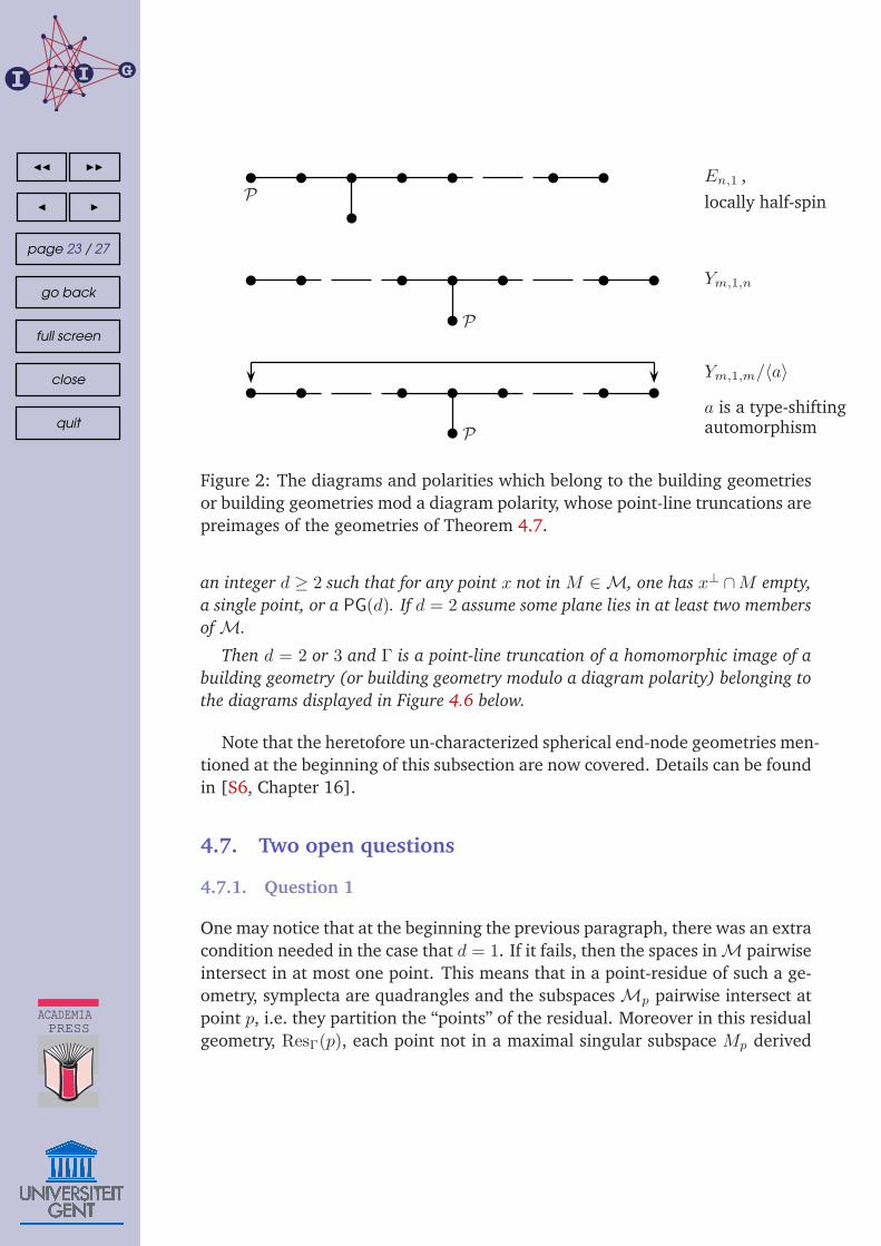
Figure 2: The diagrams and polarities which belong to the building geometries

or building geometries mod a diagram polarity, whose point-line truncations are

preimages of the geometries of Theorem 4.7.

an integer d ≥ 2 such that for any point x not in M ∈ M, one has x⊥ ∩M empty,

a single point, or a PG(d). If d = 2 assume some plane lies in at least two members

of M.

Then d = 2 or 3 and Γ is a point-line truncation of a homomorphic image of a

building geometry (or building geometry modulo a diagram polarity) belonging to

the diagrams displayed in Figure 4.6 below.

Note that the heretofore un-characterized spherical end-node geometries men-

tioned at the beginning of this subsection are now covered. Details can be found

in [S6, Chapter 16].

4.7. Two open questions

4.7.1. Question 1

One may notice that at the beginning the previous paragraph, there was an extra

condition needed in the case that d = 1. If it fails, then the spaces in M pairwise

intersect in at most one point. This means that in a point-residue of such a ge-

ometry, symplecta are quadrangles and the subspaces Mp pairwise intersect at

point p, i.e. they partition the “points” of the residual. Moreover in this residual

geometry, ResΓ(p), each point not in a maximal singular subspace Mp derived

I I G

◭◭ ◮◮

◭ ◮

page 24 / 27

go back

full screen

close

quit

ACADEMIA

PRESS

from an element of Mp, is collinear to exactly one point of Mp. One now cer-

tainly has the situation that set up Cohen’s Technical Lemma. The argument

forces convex non-grid quadrangles to exist in this geometry. But there is no

end-result showing that this picture of a point-residual cannot exist. In fact, us-

ing the notion of an admissible triple (introduced by Bart De Bruyn [DB]), one

can construct examples which fulfill all the requirements — suggesting there

was a good reason to place that condition in the theorems described above. But

the residual we are speaking of is the point-residual of a parapolar space of

symplectic rank 3, and each non-oriflamme symplecton S (recall that they must

exist) now possesses a collection of maximal singular PG(2)’s which pair-wise

meet in at most one point. In other words, they form an ovoidal hyperplane of

the dual polar space DS associated with S. We should mention that since the

elements of M are not planes, the planes of S are Desarguesian, so S (being

non-oriflamme) are classic embeddable rank 3 polar spaces. As far as the writer

knows the non-existence of such ovoidal hyperplanes has been shown only for

the finite dual-polar spaces of type W (3, q) (Cooperstein and Pasini [CP], a dif-

ficult proof using hard theorems of Woldar and Hemmeter [HW]).

My point here is simply to pin-point the connection of the ovoidal hyperplane

problem with the singular characterizations of the previous subsection when

d = 1.

4.7.2. Question 2

The conclusions of Theorems 4.5 and 4.6 overlap: They both contain the meta-

symplectic spaces. This suggests that it may be possible to prove Theorem 4.6

without invoking the local pentagon property. The reader is invited to unravel

this mystery.

References

[BT] A. Bichara and G. Tallini, On a characterization of Grassmann space rep-

resenting the h-dimensional subspaces in a projective space, Ann. Discrete

Math. 18 (1983), 113–131.

[BrC] A. E. Brouwer and A. M. Cohen, Local recognition of Tits geometries of

classical type, Geom. Dedicata 20 (1986), 181–199.

[Bu] F. Buekenhout, The basic diagram of a geometry, in Geometries and

Groups, Martin Aigner and Dieter Jungnickel (eds), pp. 1–29, Springer,

Berlin, 1981.

I I G

◭◭ ◮◮

◭ ◮

page 25 / 27

go back

full screen

close

quit

ACADEMIA

PRESS

[BSch] F. Buekenhout and W. Schwarz, A simplified version of strong connec-

tivity in geometries, J. Combin. Theory Ser. A 37 (1984), 73–75.

[BS] F. Buekenhout and E. Shult, On the foundations of polar geometry,

Geom. Dedicata 3 (1974), 155–170.

[C1] A. Cohen, An axiom system for metasymplectic spaces, Geom. Dedicata

12 (1982), 417–433.

[C2] , On a theorem of Cooperstein, European J. Combin. 4 (1983),

107–106.

[CC] A. Cohen and B. Cooperstein, A characterization of some geometries of

Lie type, Geom. Dedicata 15 (1983), 73–105.

[CS] A. Cohen and E. Shult, Affine polar spaces, Geom. Dedicata 35 (1990),

43–76.

[Cp] B. Cooperstein, A characterization of some Lie incidence structures,

Geom. Dedicata 6 (1977), 205–258.

[CP] B. Cooperstein and A. Pasini, The non-existence of ovoids in the dual

polar space DW (5, q), J. Combin. Theory Ser. A 104 (2003), 351–364.

[Cu1] H. Cuypers, On a generalization of Fischer spaces, Geom. Dedicata 34

(1990), 67–87.

[Cu2] , Affine Grassmannians, J. Combin. Theory Ser. A 70 (1995), 289–

304.

[CJP] H. Cuypers, P. Johnson and A. Pasini, On the classification of polar

spaces, J. Geom. 48 (1993), 56–62.

[CP] H. Cuypers and A. Pasini, Locally polar geometries with affine planes,

European J. Combin. 13 (1992), 39–57.

[DB] B. De Bruyn, Generalized quadrangles with a spread of symmetry, Euro-

pean J. Combin. 20 (1999), 759–771.

[DS] A. W. M. Dress and R. Scharlau, Gated sets in metric spaces, Aequationes

Math. 34 (1987), 112–120.

[ES] C. A. Ellard and E. Shult, A characterization of polar Grassmann spaces,

preprint, Kansas State University, 1988.

[HW] J. Hemmeter and A. Woldar, Classification of the maximal cliques of

size ≥ q + 4 in the quadratic forms graph in odd characteristic, European

J. Combin 11 (1990), 433–449.

I I G

◭◭ ◮◮

◭ ◮

page 26 / 27

go back

full screen

close

quit

ACADEMIA

PRESS

[J] P. Johnson, Polar spaces of arbitrary rank, Geom. Dedicata 35 (1990),

229–250.

[K] A. Kasikova, Characterizations of some subgraphs of the point-

collinearity graphs of building geometries, European J. Combin. 28

(2007), 1493–1529.

[KS1] A. Kasikova and E. Shult, Chamber systems which are not geometric,

Comm. Algebra 24 (1996), 3471–3481.

[KS2] , Point-line characterizations of Lie geometries, Adv. Geom. 2

(2002), 147–188.

[P] A. Pasini, Diagram Geometries, Oxford Science Publications, Clarendon

Press, Oxford, 1994.

[Sch] R. Scharlau, A characterization of Tits buildings by metrical properties,

J. London Math. Soc. 32 (1985), 317–327.

[S1] E. Shult, Characterizations of the Lie incidence geometries, in Surveys in

Combinatorics, London Math. Soc. Lecture Note Ser. vol. 82, ed. E. Keith

Lloyd, pp. 157–186, Cambridge University Press, Cambridge, 1983.

[S3] , Characterizations of spaces related to metasymplectic spaces,

Geom. Dedicata 30 (1991), 325–371.

[S2] , Aspects of buildings, in Groups and Geometries (Siena, 1996),

Lino Martino et al (eds.), pp. 177–188, Birkhauser, Basel, 1998.

[S4] , Characterizing the half-spin geometries by a class of singular

subspaces, Bull. Belg. Math. Soc. Simon Stevin 12 (2005), 883–894.

[S5] , Characterization of Grassmannians by one class of singular sub-

spaces, Adv. Geom. 3 (2003), 227–250.

[S6] , Points and Lines: Characterization of the Lie Incidence Geometries,

book submitted for publication.

[KT] E. E. Shult and K. Thas, A theorem of Cohen on parapolar spaces, Com-

binatorica, to appear.

[Te] L. Teirlinck, Planes and hyperplanes of 2-coverings, Bull. Belg. Math. Soc.

Simon Stevin 29 (1977), 73–81.

[TPM] J. A. Thas, S. E. Payne and H. Van Maldeghem, Half Moufang implies

Moufang for finite generalized quadrangles, Invent. Math. 105 (1991),

153–156.

I I G

◭◭ ◮◮

◭ ◮

page 27 / 27

go back

full screen

close

quit

ACADEMIA

PRESS

[T1] J. Tits, Buildings of Spherical Type and Finite BN -Pairs, Lecture Notes in

Math., vol. 386, Springer, Berlin, 1974.

[T2] , A local approach to buildings, in The Geometric Vein (the Coxeter

Festschrift), C. Davis and B. Grunbaum, and F. A. Sherk (eds.), pp. 519–

547, Springer, Berlin, 2002.

[TW] J. Tits and R. M. Weiss, Moufang Polygons, Springer Monogr. Math.,

Springer, Berlin, 2002.

[VY] O. Veblen and J. Young, Projective Geometry, Ginn, Boston, 1916.

[Vl] F. D. Veldkamp, Polar geometry, I - IV, Indag. Math. 21 (1959), 512–551.

Ernest Shult

DEPT. OF MATH., KANSAS STATE UNIV., MANHATTAN KS, 66502, USA

e-mail: ernest shult@yahoo.com